More examples of structure formation in the Lemaître-Tolman model

Abstract

In continuing our earlier research, we find the formulae needed to determine the arbitrary functions in the Lemaître-Tolman model when the evolution proceeds from a given initial velocity distribution to a final state that is determined either by a density distribution or by a velocity distribution. In each case the initial and final distributions uniquely determine the L-T model that evolves between them, and the sign of the energy-function is determined by a simple inequality. We also show how the final density profile can be more accurately fitted to observational data than was done in our previous paper. We work out new numerical examples of the evolution: the creation of a galaxy cluster out of different velocity distributions, reflecting the current data on temperature anisotropies of CMB, the creation of the same out of different density distributions, and the creation of a void. The void in its present state is surrounded by a nonsingular wall of high density.

Short title:   More examples of structure formation in LT

Phys. Rev. D, Submitted 5/3/2003, Accepted datedate

I Scope

In a previous paper KrHe2001 , which we shall call Paper I, we showed that one can uniquely define the Lemaître-Tolman cosmological model Lema1933 ; Tolm1934 by specifying an initial density profile (i.e. the mass-density as a function of the radial coordinate at an initial instant $t=t_{1}$) and a final density profile. The formulae defining the L-T functions $E(M)$ and $t_{B}(M)$ (where $M$ is the active gravitational mass, used here as a radial coordinate) are implicit but unique, and can be solved for $E$ and $t_{B}$ numerically. (For definitions of $E$ and $t_{B}$ see eqs. (2.1) and (2.2).) We also worked out a numerical example in which a galaxy-cluster-like final profile was created out of an initial profile whose density amplitude and linear size were small.

In the present paper, we develop that study for new elements: we show that instead of a density distribution, one can specify a velocity distribution (strictly speaking, this is $R_{,t}/M^{1/3}$ — a measure of the velocity) at either the initial instant or the final instant or both. We prove a theorem, analogous to the one proven in paper I: given the initial and the final profile, the L-T model that evolves between them is uniquely determined. We also show how to adapt the initial and final density profiles to the astrophysical data more precisely than it was done in paper I. We provide numerical examples of L-T evolution between an initial profile (of density or velocity) consistent with the implications of the CMB measurements, and a final profile that corresponds either to a galaxy cluster or to a void.

The paper is arranged as follows. We recall the basic properties of the L-T model in sec. 2. In sec. 3 we describe how the final profile can be adapted to observational data more exactly than in Paper I. In sec. 4 we find the implicit formulae to define the L-T functions $E(M)$ and $t_{B}(M)$ when the initial state is specified by a velocity distribution and the final state by a density distribution. In sec. 5 we do the same for both states being specified by velocity distributions. In sec. 6 we deduce the amplitude of the velocity perturbation at $t_{1}$ allowed by observations of the CMB radiation. In sec. 7 we specify our choices of density and velocity profiles for numerical investigations. Secs. 8 and 9 contain the presentation of numerical results in several figures. The results are summarized and interpreted in sec. 10, and brief conclusions follow in sec. 11.

The approach presented in this and in paper I is more suited to astrophysical practice than the traditional approach, in which we first try to deduce the initial state of the Universe from various kinds of data, and then proceed to calculate the evolution of the cosmological model, in order to compare its final state with the observations of the current state of the actual Universe. Our approach allows one to make simultaneous use of the data on the initial and on the final state of the Universe — the real astronomical data is indeed such a mixture.

Naturally the L-T model can describe the actual astrophysical process of structure formation only approximately. The obvious limitation is spherical symmetry, in consequence of which we cannot take into account the rotation of the objects formed. Thus, no matter how well we reproduce the profile of a galaxy or cluster, the L-T model will continue to evolve, and the profile will look quite different after $10^{6}$ years or less, whereas real galaxies and clusters are fairly stable over $10^{9}$ years. However, we hope that the method presented here will be a starting point for generalisations that will be done once (and if) more general exact cosmological models are discovered.

II Basic properties of the Lemaître-Tolman model.

The Lemaître-Tolman (L-T) model Lema1933 ; Tolm1934 is a spherically symmetric nonstatic solution of the Einstein equations with a dust source. Its metric is:

$$\text{d}s^{2}=\text{d}t^{2}-\frac{{R,_{r}}^{2}}{1+2E(r)}\text{d}r^{2}-R^{2}(t,r)(\text{d}\vartheta^{2}+\sin^{2}\vartheta\text{d}\varphi^{2}),$$ (2.1)

where $E(r)$ is an arbitrary function (arising as an integration constant from the Einstein equations), $R,_{r}=\partial R/\partial r$, and $R$ obeys

$${R_{,t}}^{2}=2E+2M/R+\frac{1}{3}\Lambda R^{2},$$ (2.2)

where $\Lambda$ is the cosmological constant. Eq. (2.2) is a first integral of the Einstein equations, and $M(r)$ is another arbitrary function that arises as an integration constant. The mass-density is:

$$\kappa\rho=\frac{2M,_{r}}{R^{2}R,_{r}},\qquad\text{where}\ \kappa=\frac{8\pi G}{c^{4}}.$$ (2.3)

See Kras1997 for an extensive list of properties and other work on this model. In the following, we will assume $\Lambda=0$. Then eq. (2.2) can be solved explicitly. The solutions are the following.

Elliptic case, $E<0$:

$$R(t,r)=-\frac{M}{2E}(1-\cos\eta),$$ (2.4a)

$$\eta-\sin\eta=\frac{(-2E)^{3/2}}{M}(t-t_{B}(r)).$$ (2.4b)

where $\eta$ is a parameter;

Parabolic case, $E=0$:

$$R(t,r)=\left[\frac{9}{2}M(t-t_{B}(r))^{2}\right]^{1/3},$$ (2.5)

Hyperbolic case, $E>0$:

$$R(t,r)=\frac{M}{2E}(\cosh\eta-1),$$ (2.6a)

$$\sinh\eta-\eta=\frac{(2E)^{(3/2)}}{M}(t-t_{B}(r)),$$ (2.6b)

where $t_{B}(r)$ is one more arbitrary function (the bang time). Note that all the formulae given so far are covariant under arbitrary coordinate transformations $r=g(r^{\prime})$, and so $r$ can be chosen at will. This means one of the three functions $E(r)$, $M(r)$ and $t_{B}(r)$ can be fixed at our convenience by the appropriate choice of $g$.

The Friedmann models are contained in the Lemaître-Tolman class as the limit:

$$t_{B}=\text{ const},\qquad|E|^{3/2}/M=\text{ const},$$ (2.7)

and one of the standard radial coordinates for the Friedmann model results if, in addition, the coordinates in (2.4) – (2.6) are chosen so that:

$$M=M_{0}r^{3},$$ (2.8)

where $M_{0}$ is an arbitrary constant. This implies $E/r^{2}=\text{ const}:=-k/2,\ k$ being the Robertson-Walker curvature index.

It will be convenient in most of what follows to use $M(r)$ as the radial coordinate (i.e. $r^{\prime}=M(r)$) because, in the structure formation context, one does not expect any “necks” or “bellies” where $M,_{r}=0$, and so $M(r)$ should be a strictly increasing function in the whole region under consideration. Then:

$$\kappa\rho=2/(R^{2}R,_{M})\equiv 6/(R^{3}),_{M},$$ (2.9)

from which we find

$$R^{3}(M)-R_{0}^{3}=\frac{3}{4\pi}\int_{M_{0}}^{M}\frac{du}{\rho(u)},$$ (2.10)

where $R_{0}$ and $M_{0}$ will commonly be zero.

In the present paper we will apply the L-T model to problems of a similar kind to that considered in Paper I: Connecting an initial state of the Universe (defined by either a mass-density distribution or a velocity distribution) to a final state (also defined by one of these distributions) by an L-T evolution, and in particular to the formation of galaxy-cluster-like and void-like objects out of initial perturbations of density or velocity that are small in amplitude and in some cases small in mass compared to the final object.

III Modelling the final density profile.

We will now incorporate in our models the observational data on mass distribution in galaxy clusters in a more detailed way than in Paper I.

The quantities of interest in the profile are the following: the maximal density (with the shapes we assume below and later, this will be at the center of the object), the radius of the object (assumed spherically symmetric), the mass of the object, the average density of the cosmic background, and the compensation radius (defined below).

We define the following parameters.

• $M_{m}$ — the mass of a galaxy cluster, out to some radius; to be taken from astronomical tables.

• $R_{m}$ — the radius within which the mass $M_{m}$ is contained; also to be taken from astronomical tables. In fact there may be two or more $M_{m}$–$R_{m}$ pairs available for some clusters (see section VII.3.1).

• $\rho(M_{m})=\rho_{b}d$ — this is the geometrical definition of the mass $M_{m}$ ($M=M_{m}$ at that value of $R=R_{m}$ at which $\rho$ equals a certain specified multiple of the background density). We do not assume any value of $d$ at this point yet, except that $1\leq d<\rho_{\text{max}}/\rho_{b}$.

• The compensation radius $R=R_{c}$, at which the total mass within $R=R_{c}$ is the same as the background mass would be if no inhomogeneity were created. This is needed to let us know roughly where our inhomogeneity is matched to the Friedmann background. See subsection III.1.

III.1 Compensation Radius & Mass

The matching of contained mass at $R_{c}$ is not sufficient for a Swiss-cheese type matching, as we have not required the time since the bang to match up at this location, and therefore is technically the wrong definition. However, it has the advantage that it can be calculated knowing only the density profile at a given time, and under the circumstances used here is a fairly good estimate. All our models are then calculated out to $M_{c}$, i.e $0\leq M\leq M_{c}$.

We can put upper and lower limits on the compensation radius and mass. For a condensation of measured mass $M_{m}$, the $M_{c}$ value obviously cannot be less than this. In fact the region around the visible condensation, though of low density is of large volume, and will add noticeably to the mass to be ‘compensated for’. Therefore,

$$M_{c,\text{min}}>M_{m}~{},~{}~{}~{}~{}~{}~{}~{}~{}R_{c,\text{min}}>\left(\frac{3M_{m}}{4\pi\rho_{b,\text{today}}}\right)^{1/3},$$ (3.1)

where eq. (7.2) gives $\rho_{b,\text{today}}=4.075\times 10^{-30}$ g/cc. in the chosen parabolic background, or more conveniently

$$R_{c,\text{min}}>1.58\times 10^{-4}(M_{m}/M_{\odot})^{1/3}~{}\text{in Mpc}.$$ (3.2)

On the other hand, the observed average separation of condensations puts an upper limit on $R_{c}$. Since the contents of the universe are a mixed bag of galaxy clusters, rich clusters, superclusters, field galaxies, voids, walls, etc, the average separation of rich clusters say is not meaningful for this purpose. So we instead argue that there are around $3\times 10^{6}$ large galaxies & $3\times 10^{7}$ dwarf galaxies within $10^{9}$ light years. At say $10^{11}~{}M_{\odot}$ and $10^{10}~{}M_{\odot}$, respectively, this gives a mean density of around $4.97\times 10^{9}~{}M_{\odot}/$Mpc${}^{3}=3.36\times 10^{-28}$ kg/m${}^{3}=0.0826\rho_{b,\text{today}}$. Therefore an object of mass $M_{m}$ in $M_{\odot}$ should on average occupy a volume of radius about

$$R_{c,\text{max}}=3.64\times 10^{-4}(M_{m}/M_{\odot})^{1/3}~{}\text{in Mpc}.$$ (3.3)

For a galaxy of $10^{11}~{}M_{\odot}$, these two limits are $0.735<R_{c}<1.69$ Mpc, whereas for an Abell Cluster of $10^{15}~{}M_{\odot}$, these two limits are $15.8<R_{c}<36.4$ Mpc.

For a void, the interior density will not be zero, but is not well known, and the radius is of the order of 60 Mpc. Only by including some of the galaxies in the surrounding walls can one bring the average density up to the background value. So $R_{c}>60$ Mpc, which at background density gives $M_{c}>5.5\times 10^{16}~{}M_{\odot}$.

III.2 An example of fitting a profile.

Since little is known about mass-distribution within galaxy clusters, we cannot attempt to model any actual cluster to any significant accuracy. However, we wish to show that such modelling is in principle possible. Therefore, for the beginning, we will use the profile from Paper I and will show below that its free parameters can be made equal to some observed/observable quantities.

Let $\rho_{b}$ be the background density. We choose the profile at $t_{2}$ to be

$$\rho(M)=B_{2}\rho_{b}\text{e}^{-(M/\mu_{2})^{2}},$$ (3.4)

where $B_{2}$ and $\mu_{2}$ are free parameters to be adapted to the observational constraints.

Given two pairs of $(M_{m},R_{m})$ data, $(M_{a},R_{a})$ & $(M_{b},R_{b})$, we have

$$R^{3}=\frac{3\mu_{2}}{8\sqrt{\pi}\;B_{2}\rho_{b}}\text{erfi}(M/\mu_{2})$$ (3.5)

for each of them, and each can be solved for $B_{2}$, so that:

$$\frac{3\mu_{2}\text{erfi}(M_{a}/\mu_{2})}{8\sqrt{\pi}\;R_{a}^{3}\rho_{b}}=B_{2}=\frac{3\mu_{2}\text{erfi}(M_{b}/\mu_{2})}{8\sqrt{\pi}\;R_{b}^{3}\rho_{b}}.$$ (3.6)

This is solved numerically for $\mu_{2}$, and $B_{2}$ follows.

The compensation radius $R_{c}$ is determined by the condition that the mean density out to $M$ equals the background density:

$$\rho_{b}=\frac{M_{c}}{4\pi R(M_{c})^{3}/3}=\frac{2B_{2}\rho_{b}M_{c}}{\sqrt{\pi}\;\mu_{2}\text{erfi}(M_{c}/\mu_{2})}.$$ (3.7)

This is solved for $M_{c}$ numerically, and $R_{c}$ follows from (3.5).

III.3 Profiles inspired by astronomy.

We looked for density profiles that are considered realistic by astronomers. As it turned out, there is no general agreement as to which profile best describes observations, and no generally accepted definition of the radius of a galaxy cluster exists. However (see the Acknowledgements) the following ‘universal profile’ is one of the more commonly used formulas for density vs. distance profiles NaFW1995 ; NaFW1996 ; NaFW1997 :

$$\rho(\zeta)=\rho_{b}\delta\frac{1}{(\zeta/\zeta_{s})(1+\zeta/\zeta_{s})^{2}},$$ (3.8)

where $\rho_{b}$ is the average density in the Universe, $\delta$ is a dimensionless factor and $\zeta_{s}$ is a scale distance. (This is a Newtonian formula, in which $\zeta$ is the Euclidean distance.) According to the authors of Refs. NaFW1995 ; NaFW1996 ; NaFW1997 , this profile applies for $\zeta$ changing by two orders of magnitude.

For our procedure, we need the density given as a function of mass, which cannot be found analytically for the above profile. The calculation $\rho(\zeta)\rightarrow M(\zeta)\rightarrow\zeta(M)\rightarrow\rho(M)$ can always be done numerically, but it is more instructive to have exact explicit formulae.

We therefore approximate $M(\zeta)$ separately in the ranges $\zeta\ll\zeta_{s}$ and $\zeta\gg\zeta_{s}$.

For $\zeta\ll\zeta_{s}$ a Taylor series around $\zeta=0$ up to $\zeta^{2}$ gives

$$M(\zeta)\approx 2\pi\rho_{b}\delta\zeta_{s}\zeta^{2}:=\beta^{2}\zeta^{2}~{}~{}~{}~{}\rightarrow~{}~{}~{}~{}\zeta\approx\sqrt{M}/\beta.$$ (3.9)

which converts the profile (3.8) to:

$$\rho_{1}(M)=\rho_{b}\beta\delta\zeta_{s}\frac{1}{\sqrt{M}\left(1+\frac{\sqrt{M}}{\beta\zeta_{s}}\right)^{2}}.$$ (3.10)

Like the original profile, this one has the unpleasant property that the density becomes infinite at $M\to 0$, so we modify it to

$$\rho_{2}(M)=\frac{\rho_{b}\beta\delta\zeta_{s}}{(\epsilon+\sqrt{M})\left(1+\frac{\sqrt{M}}{\beta\zeta_{s}}\right)^{2}}.$$ (3.11)

where $\epsilon$ is small compared to $\beta\delta\zeta_{s}$, and this can be integrated to give $R(M)$.

When $\zeta\gg\zeta_{s}$, the approximation

$$\begin{split}M(\zeta)\approx 4\pi\rho_{b}\delta\zeta_{s}\ln\left(1+\zeta/\zeta_{s}\right):=\gamma\ln\left(1+\zeta/\zeta_{s}\right),\\ ~{}~{}~{}~{}\rightarrow~{}~{}~{}~{}\zeta=\zeta_{s}\left(\text{e}^{M/\gamma}-1\right),\end{split}$$ (3.12)

substituted into (3.8) gives

$$\rho_{4}(M)=\rho_{b}\frac{\delta}{\text{e}^{M/\gamma}-1+\nu}\text{e}^{-2M/\gamma}$$ (3.13)

where $\nu$ has again been added into the denominator to permit a non-divergent central density. The corresponding $R^{3}(M)$ is still elementary.

The profiles (3.11) and (3.13) were the starting point for our considerations. The profiles actually used in numerical examples were various modifications of these (see Sec. VII), done in order to better fit our profiles to observational data.

III.4 The initial density profile.

We assume that the condensed object (model of a galaxy cluster) was created out of a small localized initial density or velocity perturbation, superimposed on the homogeneous spatially flat Friedmann background. During the evolution, the perturbation was increasing in density amplitude and in mass, and thus was effectively drawing more mass into the condensation region out of the surrounding homogeneous region.

At $t=t_{1}$, the profile need not be compensated. For an uncompensated profile, it is good if it is localized (i.e. the perturbation is zero for $M>M_{1}$, where $M_{1}$ is the assumed mass of the initial perturbation). Then the definitions of the radius and mass of the perturbation are straightforward.

We choose for this profile the cosine shape

$$\rho(M)=\left\{\begin{array}[]{ll}B_{1}(1+\cos(\pi M/M_{1}))+\rho_{b}&\text{~{}~{}for~{}}M\in[0,M_{1}];\\ \rho_{b}=\text{const}&\text{~{}~{}for~{}}M\geq M_{1}\end{array}\right.$$ (3.14)

with $B_{1}>0$. Then $\rho(0)=\rho_{b}(1+A)$ is the maximal value of density, with $\Delta\rho/\rho_{b}=A=2B_{1}/\rho_{b}$ being the density amplitude from astronomical data, while $M_{1}$ is the total mass of the initial perturbation.

The radius $R(M)$ is given from eq. (2.10) by

$$\begin{split}&R^{3}(M)=\frac{3M_{1}}{2\pi^{2}\sqrt{\rho_{b}\left(\rho_{b}+2B_{1}\right)}}\times\\ &\times\arctan\left[\sqrt{\frac{\rho_{b}}{\rho_{b}+2{B_{1}}}}\tan\left(\frac{\pi M}{2M_{1}}\right)\right]\quad\text{for~{}}M\leq M_{1},\end{split}$$ (3.15)

$$\begin{split}R^{3}(M)=\frac{3M_{1}}{4\pi\sqrt{\rho_{b}\left(\rho_{b}+2B_{1}\right)}}+\frac{3}{4\pi\rho_{b}}\left(M-M_{1}\right)\\ \text{for~{}}M\geq M_{1},\end{split}$$ (3.16)

where the first term on the right in (3.16) is the common value of $R^{3}$ at $M=M_{1}$.

We did one run with this kind of initial profile ($\rho$i4 in Table LABEL:InFnDenProfileTab) in order to demonstrate more clearly the point we made in Paper I: that the mass of the “seed” structure existing at time $t_{1}$ can be much smaller than the mass of the galaxy cluster into which it will evolve. The other initial profiles are either flat (see Table LABEL:RunList and Sec. X for reasons why) or go into the background only asymptotically.

IV The evolution from a given velocity distribution to a given density distribution.

The quantity that is a measure of the velocity distribution of the dust in an L-T model is

$$b=R_{,t}/M^{1/3}.$$ (4.1)

This is constant in any Robertson-Walker model, so its nonconstancy is a measure of the velocity inhomogeneity.

Suppose we wish to adapt an L-T model to a given initial velocity distribution $b=b_{1}(r)$ at $t=t_{1}$, and to a given density distribution $\rho=\rho_{2}(r)$ at $t=t_{2}$. This is a different set of data from the one considered in paper I, and so the existence of such an evolution has to be proven. The functions appearing along the way are different, but the overall mathematical scheme is essentially the same. As before, we will mostly be using the mass $M$ as the radial coordinate, and in each case we will assume that at the initial instant $t_{1}$ the configuration is expanding, so

$$R_{,t}(t_{1},M)>0\Longrightarrow b_{1}(M)>0.$$ (4.2)

Analogous reasoning can be carried out for matter that is initially collapsing, but this situation is just covered by the time reverse of the method given here and is not relevant for the problem of structure formation.

IV.1 Hyperbolic evolution.

We have, for $E>0$:

$$R_{,t}=\frac{M}{\sqrt{2E}R}\sqrt{(1+2ER/M)^{2}-1}.$$ (4.3)

If

$$\left.R_{,t}/M^{1/3}\right|_{t=t_{1}}=b_{1}(r)$$ (4.4)

is the data, then denoting $R|_{t=t_{1}}=R_{1}$ and solving the above for $R_{1}$ we find

$$R_{1}=\frac{2M^{1/3}}{{b_{1}}^{2}-2E/M^{2/3}},$$ (4.5)

and so from the evolution equations

$$\begin{split}\eta_{1}&=\text{arcosh}(1+2ER_{1}/M)\\ &=\text{arcosh}\left(\frac{{b_{1}}^{2}+2E/M^{2/3}}{{b_{1}}^{2}-2E/M^{2/3}}\right),\end{split}$$ (4.6)

$$\begin{split}&\sqrt{\left(\frac{{b_{1}}^{2}+2E/M^{2/3}}{{b_{1}}^{2}-2E/M^{2/3}}\right)^{2}-1}-\text{arcosh}\left(\frac{{b_{1}}^{2}+2E/M^{2/3}}{{b_{1}}^{2}-2E/M^{2/3}}\right)\\ &=\frac{(2E)^{3/2}}{M}\left(t_{1}-t_{B}\right).\end{split}$$ (4.7)

This is the equation that will be used as initial data at $t=t_{1}$.

The equation at $t=t_{2}$ will be the same as eq. (3.3) in paper I for $i=2$ viz:

$$\begin{split}&\sqrt{\left(1+2ER_{2}/M\right)^{2}-1}-\text{arcosh}(1+2ER_{2}/M)\\ &=\frac{(2E)^{3/2}}{M}\left(t_{2}-t_{B}\right).\end{split}$$ (4.8)

Here, the quantity $R_{2}=R(t_{2},r)$ is calculated from the given $\rho_{2}(r)=\rho(t_{2},r)$ using eq. (2.10).

Just as in paper I, we introduce the symbols

$$x=2E/M^{2/3},\qquad a_{2}=R(t_{2},M)/M^{1/3}.$$ (4.9)

The set of equations to determine $E(M)$ and $t_{B}(M)$ is then (from (4.7) and (4.8)):

$$\sqrt{\left(\frac{{b_{1}}^{2}+x}{{b_{1}}^{2}-x}\right)^{2}-1}-\text{arcosh}\left(\frac{{b_{1}}^{2}+x}{{b_{1}}^{2}-x}\right)=x^{3/2}\left(t_{1}-t_{B}\right),$$ (4.10)

$$\sqrt{\left(1+a_{2}x\right)^{2}-1}-\text{arcosh}\left(1+a_{2}x\right)=x^{3/2}\left(t_{2}-t_{B}\right),$$ (4.11)

From (4.11) we now find $t_{B}$:

$$t_{B}=t_{2}-\frac{1}{x^{3/2}}\left[\sqrt{\left(1+a_{2}x\right)^{2}-1}-\text{arcosh}(1+a_{2}x)\right],$$ (4.12)

and substituting this in (4.10) we obtain the following equation to determine $x$:

$$\Phi_{H}(x)=0,$$ (4.13)

where

$$\begin{split}\Phi_{H}(x):=&\sqrt{\left(1+a_{2}x\right)^{2}-1}-\sqrt{\left(\frac{{b_{1}}^{2}+x}{{b_{1}}^{2}-x}\right)^{2}-1}\\ &-\text{arcosh}(1+a_{2}x)+\text{arcosh}\left(\frac{{b_{1}}^{2}+x}{{b_{1}}^{2}-x}\right)\\ &-x^{3/2}\left(t_{2}-t_{1}\right).\end{split}$$ (4.14)

We will use the functions $b_{1}(M)$ and $a_{2}(M)$ implied by the assumed $R_{,t1}(M)$ and $\rho_{2}(M)$ to find $E(M)$ and $t_{B}(M)$, and then to find $\rho(t_{1},M)$. This will tell us about the relative importance of the velocity and density distributions for structure formation. In particular, with $b_{1}$ = const, the $\rho(t_{1},M)$ will tell how big the initial density inhomogeneity has to be when the initial velocity distribution is exactly homogeneous, while the final structure is given.

IV.1.1 Conditions for solutions to exist

Now we have to verify whether the equation $\Phi_{H}(x)=0$ determines a value of $x$. We see that $\Phi_{H}(x)$ is defined in the range

$$0\leq x<{b_{1}}^{2}.$$ (4.15)

It is easily seen that $\Phi_{H}(0)=0$. For $x\to{b_{1}}^{2}$, the second and fourth term in (4.14) tend to $(-\infty)$ and to $(+\infty)$, respectively, while all the other terms are finite. Since

$$\lim_{x\to{b_{1}}^{2}}\frac{\text{arcosh}\left[\left({b_{1}}^{2}+x\right)/\left({b_{1}}^{2}-x\right)\right]}{\sqrt{\left[\left({b_{1}}^{2}+x\right)/\left({b_{1}}^{2}-x\right)\right]^{2}-1}}=0,$$ (4.16)

the second term is dominant. Hence:

$$\lim_{x\to{b_{1}}^{2}}\Phi_{H}(x)=-\infty.$$ (4.17)

We also have

$$\begin{split}\Phi_{H,x}(x)&=\sqrt{x}\left[\frac{{a_{2}}^{3/2}}{\sqrt{2+a_{2}x}}-\frac{2b_{1}}{\left({b_{1}}^{2}-x\right)^{2}}-\frac{3}{2}\left(t_{2}-t_{1}\right)\right]\\ &:=\sqrt{x}\lambda_{H}(x).\end{split}$$ (4.18)

Since $\lambda_{H,x}=-\frac{1}{2}{a_{2}}^{5/2}/(2+a_{2}x)^{3/2}-4b_{1}/({b_{1}}^{2}-x)^{3}<0$, the function $\lambda_{H}(x)$ is strictly decreasing and may have at most one zero. Hence, $\Phi_{H,x}$ can be positive anywhere only if $\lambda_{H}(0)>0$, i.e. if

$$t_{2}-t_{1}<\frac{\sqrt{2}}{3}{a_{2}}^{3/2}-\frac{4}{3{b_{1}}^{3}}.$$ (4.19)

Since we consider the evolution from $t_{1}$ to $t_{2}$, it is natural to assume $t_{2}>t_{1}$. Then, (4.19) can be fulfilled only if

$$2/a_{2}<{b_{1}}^{2}.$$ (4.20)

This inequality is easy to understand if we use (4.5) for ${b_{1}}^{2}$ (with $R=R_{1}$), and recall the definition of $a_{2}$, eq. (4.9). Then (4.20) is equivalent to

$$\frac{2}{R_{2}}<\frac{2}{R_{1}}+\frac{2E}{M}.$$ (4.21)

This in turn implies that $R_{2}>R_{1}$; otherwise there will be no $E>0$ evolution from $R_{1}$ to $R_{2}$. Thus, in passing, we have proven the intuitively obvious:

Conclusion: If matter is expanding at $t=t_{1}$, then an $E>0$ L-T evolution from $R(t_{1},M)$ to $R(t_{2},M)$ will exist only if $R(t_{2},M)>R(t_{1},M)$.   o   

Note that $R(t_{2},M)>R(t_{1},M)$ does not imply $\rho(t_{2},M)<\rho(t_{1},M)$, contrary to the intuitive expectation, and in contrast to the Friedmann models. This point is discussed in Appendix B.

Eq. (4.19) may be rewritten as

$$a_{2}>\left[\frac{9}{2}\left(t_{2}-t_{1}+\frac{4}{3{b_{1}}^{3}}\right)^{2}\right]^{1/3},$$

which means that between $t_{1}$ and $t_{2}$ the model must have expanded by more than the $E=0$ model would have done. (Applying the definitions (4.4) and (4.9) to (2.5) and (4.5) for the $E=0$ case shows $t_{1}-4/(3{b_{1}}^{3})=t_{B}$ and $a_{2}=[(9/2(t_{2}-t_{B})^{2}]^{1/3}$.)

If (4.19) is fulfilled, then $\Phi_{H}(x)$ starts as an increasing function in some neighbourhood of $x=0$, beyond which there is exactly one maximum, and finally it decreases to $-\infty$ at $x={b_{1}}^{2}$, thus passing (only once) through a zero value somewhere between the maximum and $x={b_{1}}^{2}$. Hence, eqs. (4.19) and (4.20) are a necessary and sufficient condition for the existence of an $E>0$ L-T evolution connecting the initial state (defined by the velocity distribution (4.4)) to the final state defined by the density distribution $\rho_{2}(M)$. As before, the resulting model will have to be checked for the possible existence of shell-crossings and regular maxima or minima.

IV.2 Elliptic evolution; the final state in the expansion phase.

Assuming that the initial state at $t=t_{1}$ is in the expansion phase of the Universe, we find, similarly as in (4.3), that with $E<0$

$$R_{,t}=\frac{M}{\sqrt{-2E}R}\sqrt{1-(1+2ER/M)^{2}},$$ (4.22)

and then, using (4.4) we obtain (4.5) once again. Since this time $E<0$, the inequality $2M^{1/3}/R+2E/M^{2/3}\geq 0$ has to be fulfilled, but this is identical to $2M/R+2E\geq 0$ that has to hold for an $E<0$ evolution anyway. In place of (4.6) – (4.7) we obtain at $t=t_{1}$

$$\eta=\arccos\left(\frac{{b_{1}}^{2}+2E/M^{2/3}}{{b_{1}}^{2}-2E/M^{2/3}}\right),$$ (4.23)

$$\begin{split}&\arccos\left(\frac{{b_{1}}^{2}+2E/M^{2/3}}{{b_{1}}^{2}-2E/M^{2/3}}\right)-\sqrt{1-\left(\frac{{b_{1}}^{2}+2E/M^{2/3}}{{b_{1}}^{2}-2E/M^{2/3}}\right)^{2}}\\ &=\frac{(-2E)^{3/2}}{M}\left(t_{1}-t_{B}\right).\end{split}$$ (4.24)

Since we assumed the final state at $t=t_{2}$ to be in the expansion phase, too, the equation at $t=t_{2}$ is the same as eq. (3.15) in paper I for $i=2$:

$$\begin{split}&\arccos\left(1+2ER_{2}/M\right)-\sqrt{1-\left(1+2ER_{2}/M\right)^{2}}\\ &=\frac{(-2E)^{3/2}}{M}\left(t_{2}-t_{B}\right).\end{split}$$ (4.25)

We introduce $a_{2}$ by (4.9) and

$$x=-2E/M^{2/3},$$ (4.26)

then (4.24) and (4.25) become

$$\arccos\left(\frac{{b_{1}}^{2}-x}{{b_{1}}^{2}+x}\right)-\sqrt{1-\left(\frac{{b_{1}}^{2}-x}{{b_{1}}^{2}+x}\right)^{2}}=x^{3/2}\left(t_{1}-t_{B}\right),$$ (4.27)

$$\arccos\left(1-a_{2}x\right)-\sqrt{1-\left(1-a_{2}x\right)^{2}}=x^{3/2}\left(t_{2}-t_{B}\right).$$ (4.28)

From (4.28) we have

$$t_{B}=t_{2}-\frac{1}{x^{3/2}}\left[\arccos\left(1-a_{2}x\right)-\sqrt{1-\left(1-a_{2}x\right)^{2}}\right],$$ (4.29)

and substituting this in (4.27) we obtain

$$\Phi_{X}(x)=0,$$ (4.30)

where

$$\begin{split}\Phi_{X}(x):=&\sqrt{1-\left(\frac{{b_{1}}^{2}-x}{{b_{1}}^{2}+x}\right)^{2}}-\sqrt{1-\left(1-a_{2}x\right)^{2}}\\ &+\arccos\left(1-a_{2}x\right)-\arccos\left(\frac{{b_{1}}^{2}-x}{{b_{1}}^{2}+x}\right)\\ &-x^{3/2}\left(t_{2}-t_{1}\right).\end{split}$$ (4.31)

The terms containing $b_{1}$ do not impose any extra restriction on $x$ apart from $x>0$ that follows from the definition (4.26). Since $a_{2}>0$ and $x>0$, the restriction on $x$ imposed by the other terms is the same as in paper I:

$$x\leq 2/a_{2},$$ (4.32)

which follows from $2M/R+2E\geq 0$ ($x=2/a_{2}$ corresponds to the given $M$-shell being exactly at the maximum of expansion at $t=t_{2}$).

IV.2.1 Conditions for solutions to exist

The calculations are similar to those in the previous subsection, they are described in Appendix C.1. Eq. (4.30) has a solution if and only if the following two inequalities are obeyed:

$$t_{2}-t_{1}>\frac{\sqrt{2}}{3}{a_{2}}^{3/2}-\frac{4}{3{b_{1}}^{3}},$$ (4.33)

which is the opposite of (4.19), and

$$\begin{split}&t_{2}-t_{1}\leq\\ &\left(a_{2}/2\right)^{3/2}\left[\pi+\frac{b_{1}\sqrt{2a_{2}}}{a_{2}{b_{1}}^{2}/2+1}-\arccos\left(\frac{a_{2}{b_{1}}^{2}/2-1}{a_{2}{b_{1}}^{2}/2+1}\right)\right].\end{split}$$ (4.34)

The solution is then unique. The second inequality is equivalent to eq. (3.22) in paper I, as can be verified by writing (4.5) as $b_{1}=\sqrt{2/a_{1}-x}$ and using $x=2/a_{2}$.

It follows that the right-hand side of (4.34) is always greater than the right-hand side of (4.33), as proven in Appendix A to paper I, so the two inequalities (4.34) and (4.33) are consistent. It follows further, as shown in paper I, that the equality in (4.34) means that the final state at $t_{2}$ is exactly at the maximum expansion. Note that, in consequence of $b_{1}>0,a_{2}>0$ and $\arccos(\text{anything})\leq\pi$, the right-hand side of (4.34) is always positive, and so, given $t_{1}$, values of $t_{2}$ obeying (4.34) always exist.

The set of inequalities (4.33) – (4.34) constitutes the necessary and sufficient condition for the existence of an $E<0$ L-T evolution between the initial state at $t_{1}$ specified by the velocity distribution (4.4) and the final state at $t_{2}$ specified by the density distribution $\rho(t_{2},M)=\rho_{2}(M)$, such that the final state is still in the expansion phase.

IV.3 Elliptic evolution; the final state in the recollapse phase.

We assume now that the initial state at $t=t_{1}$ is again in the expansion phase, so eqs. (4.22) – (4.24) still apply. However, the final state at $t=t_{2}$ is now assumed to be in the recollapse phase. Instead of eq. (4.25) we then get

$$\begin{split}&\pi+\arccos\left(-1-2ER_{2}/M\right)+\sqrt{1-\left(1+2ER_{2}/M\right)^{2}}\\ &=\frac{(-2E)^{3/2}}{M}\left(t_{2}-t_{B}\right).\end{split}$$ (4.35)

Introducing again $a_{2}$ by (4.9) and $x$ by (4.26), we obtain the set of equations consisting of (4.27) and

$$\begin{split}&\pi+\arccos\left(-1-a_{2}x\right)+\sqrt{1-\left(1-a_{2}x\right)^{2}}\\ &=x^{3/2}\left(t_{2}-t_{B}\right).\end{split}$$ (4.36)

The solution for $t_{B}$ is now

$$\begin{split}&t_{B}=t_{2}\\ &-\frac{1}{x^{3/2}}\left[\pi+\arccos\left(-1+a_{2}x\right)+\sqrt{1-\left(1-a_{2}x\right)^{2}}\right],\end{split}$$ (4.37)

and substituting this in (4.27) we get

$$\Phi_{C}(x)=0,$$ (4.38)

where

$$\begin{split}\Phi_{C}(x):=&\sqrt{1-\left(\frac{{b_{1}}^{2}-x}{{b_{1}}^{2}+x}\right)^{2}}+\sqrt{1-\left(1-a_{2}x\right)^{2}}\\ &+\pi-\arccos\left(\frac{{b_{1}}^{2}-x}{{b_{1}}^{2}+x}\right)+\arccos\left(-1+a_{2}x\right)\\ &-x^{3/2}\left(t_{2}-t_{1}\right).\end{split}$$ (4.39)

As before, we have $x>0$ by definition and $x\leq 2/a_{2}$.

IV.3.1 Condition for solutions to exist

The details of the calculation are shown in Appendix C.2. Eq. (4.38) has a solution if and only if

$$\begin{split}t_{2}-t_{1}\geq\left(a_{2}/2\right)^{3/2}\left[\pi+\frac{b_{1}\sqrt{2a_{2}}}{a_{2}{b_{1}}^{2}/2+1}\right.\\ \left.-\arccos\left(\frac{a_{2}{b_{1}}^{2}/2-1}{a_{2}{b_{1}}^{2}/2+1}\right)\right],\end{split}$$ (4.40)

and then the solution is unique. This is the necessary and sufficient condition for the existence of an $E<0$ L-T evolution between the initial state at $t_{1}$ specified by the velocity distribution (4.4) and the final state at $t_{2}$ specified by the density distribution $\rho(t_{2},M)=\rho_{2}(M)$, such that the final state is in the recollapse phase.

IV.4 A note on the meaning of parameters.

It should be noted that the values of the time coordinate $t_{1}$ and $t_{2}$, at which the initial and final states are specified, do not play individual roles in the calculations. The meaningful parameter is $(t_{2}-t_{1})$; it is this value that determines $E(M)$, and then the corresponding $t_{B}$ is calculated. The “age of the Universe” at the two instants then follows, being $(t_{1}-t_{B})$ and $(t_{2}-t_{B})$, respectively. This conclusion applies as well to paper I; and the same is still true in the Friedmann limit, where $x$, $a_{1}$, $a_{2}$ and $b_{1}$ are no longer functions of $M$, but just constants. Hence, the physical input data for the procedure, both here and in paper I, are the initial and final distributions of density or velocity and the time-interval between them, $(t_{2}-t_{1})$. The individual values of $t_{1}$ and $t_{2}$ do not have a physical meaning.

V The evolution from a given velocity distribution to another velocity distribution.

For completeness, we shall also consider the case when both the initial and the final state are defined by velocity distributions, even though this does not seem to be directly useful for astrophysics.

V.1 Hyperbolic evolution.

Eq. (4.7) still applies. Defining $x=2E/M^{2/3}$ as in the previous cases, we again obtain eq. (4.10), while instead of (4.11) we now have

$$\sqrt{\left(\frac{{b_{2}}^{2}+x}{{b_{2}}^{2}-x}\right)^{2}-1}-\text{arcosh}\left(\frac{{b_{2}}^{2}+x}{{b_{2}}^{2}-x}\right)=x^{3/2}\left(t_{2}-t_{B}\right),$$ (5.1)

where

$$\left.b_{2}=R_{,t}/M^{2/3}\right|_{t=t_{2}}.$$ (5.2)

Since the hyperbolic expansion cannot be reversed to become collapse, and since we assumed $b_{1}>0$ (expansion rather than collapse at $t_{1}$), it follows that $b_{2}>0$ is a necessary condition here.

From (4.10) and (5.1) we obtain two equations

$$\begin{split}t_{B}=&t_{i}-\frac{1}{x^{3/2}}\left[\sqrt{\left(\frac{{b_{i}}^{2}+x}{{b_{i}}^{2}-x}\right)^{2}-1}-\text{arcosh}\left(\frac{{b_{i}}^{2}+x}{{b_{i}}^{2}-x}\right)\right],\\ &i=1,2,\end{split}$$ (5.3)

so $x$ is the solution of

$$\chi_{H}=0,$$ (5.4)

where

$$\begin{split}\chi_{H}(x):=&\sqrt{\left(\frac{{b_{2}}^{2}+x}{{b_{2}}^{2}-x}\right)^{2}-1}-\sqrt{\left(\frac{{b_{1}}^{2}+x}{{b_{1}}^{2}-x}\right)^{2}-1}\\ &-\text{arcosh}\left(\frac{{b_{2}}^{2}+x}{{b_{2}}^{2}-x}\right)+\text{arcosh}\left(\frac{{b_{1}}^{2}+x}{{b_{1}}^{2}-x}\right)\\ &-x^{3/2}\left(t_{2}-t_{1}\right).\end{split}$$ (5.5)

Note that (4.5) and its analogue at $t_{2}$ imply ${b_{i}}^{2}-x\equiv 2/a_{i}>0$, $i=1,2$, i.e. $x<{b_{i}}^{2}$ at both $i=1$ and $i=2$. This, together with $x>0$, guarantees that the argument of arcosh will be always $\geq 1$, as it should be. Simultaneously, it guarantees that both square roots will be real.

V.1.1 Conditions for solutions to exist

Details of the calculations are shown in Appendix C.2.

For further analysis, we will need to investigate the derivative of $\chi_{H}(x)$, it is

$$\begin{split}\frac{\text{d}}{\text{d}x}\chi_{H}(x)&=\sqrt{x}\left[\frac{2b_{2}}{\left({b_{2}}^{2}-x\right)^{2}}-\frac{2b_{1}}{\left({b_{1}}^{2}-x\right)^{2}}-\frac{3}{2}\left(t_{2}-t_{1}\right)\right]\\ &:=\sqrt{x}\mu_{H}(x).\end{split}$$ (5.6)

We also have to know which of ${b_{1}}^{2}$, ${b_{2}}^{2}$ is greater. As expected, it turns out that in consequence of the assumptions made ($t_{2}>t_{1}$ and $\left.R_{,t}\right|_{t=t_{1}}>0$, i.e. $b_{1}>0$), ${b_{1}}^{2}$ must be greater, or else the $E>0$ evolution between the two states will not exist — see Appendix D.

Therefore we take it for granted that

$$b_{1}>b_{2},$$ (5.7)

i.e. that at every point the velocity of expansion at $t_{2}$ must be smaller than at $t_{1}$ at the same comoving coordinate $M$. With $b_{1}>b_{2}$, we have

$$x<{b_{2}}^{2},\qquad\lim_{x\to{b_{2}}^{2}}\mu_{H}(x)=+\infty,$$ (5.8)

and, in a similar way as in Appendix D, it can be proven that now $\mu^{\prime}_{H}(x)>0$ for all $x>0$. Consequently, $\mu_{H}(x)$ may have at most one zero, and it will have one only if $\mu_{H}(0)<0$, i.e. if

$$t_{2}-t_{1}>\frac{4}{3}\left(\frac{1}{{b_{2}}^{3}}-\frac{1}{{b_{1}}^{3}}\right).$$ (5.9)

Unlike in those cases where the profile was specified by density, the time-difference between the initial and the final state must be sufficiently large. The inequality becomes more intelligible when it is rewritten as

$${b_{2}}^{3}>\frac{{b_{1}}^{3}}{1+\frac{3}{4}{b_{1}}^{3}\left(t_{2}-t_{1}\right)},$$ (5.10)

which means that an $E>0$ evolution between the two states will exist provided the velocity of expansion at $t_{2}$ is greater than the velocity of expansion of the $E=0$ model, for which $b^{3}=4/[3(t-t_{B})]$, giving an equality in (5.10).

Since the range of $x$ is limited to $(0,{b_{2}}^{2})$, finding $x$ numerically will pose no problems.

V.2 Elliptic evolution, the final state in the expansion phase.

Expansion at $t_{2}$ is equivalent to $b_{2}>0$. The set of equations to define $x=-2E/M^{2/3}$ now consists of (4.27) and its analogue at $t_{2}$, obtained by the substitution $(b_{1},t_{1})\to(b_{2},t_{2})$. Hence:

$$\begin{split}t_{B}=&t_{i}-\frac{1}{x^{3/2}}\left[\arccos\left(\frac{{b_{i}}^{2}-x}{{b_{i}}^{2}+x}\right)-\sqrt{1-\left(\frac{{b_{i}}^{2}-x}{{b_{i}}^{2}+x}\right)^{2}}\right],\\ &i=1,2,\end{split}$$ (5.11)

and $x$ satisfies

$$\chi_{X}(x)=0,$$ (5.12)

where

$$\begin{split}\chi_{X}(x):=&-\sqrt{1-\left(\frac{{b_{2}}^{2}-x}{{b_{2}}^{2}+x}\right)^{2}}+\sqrt{1-\left(\frac{{b_{1}}^{2}-x}{{b_{1}}^{2}+x}\right)^{2}}\\ &+\arccos\left(\frac{{b_{2}}^{2}-x}{{b_{2}}^{2}+x}\right)-\arccos\left(\frac{{b_{1}}^{2}-x}{{b_{1}}^{2}+x}\right)\\ &-x^{3/2}\left(t_{2}-t_{1}\right).\end{split}$$ (5.13)

This time there is no additional limitation imposed on $x$ by eqs. (5.11) – (5.13) — the square roots and the arccos will be well-defined for every value of $x>0$. The relation between $x$ and $b_{i}$ is $x=2M^{1/3}/\left[R_{i}\left({b_{i}}^{2}+1\right)\right]$, and so indeed any value of $x>0$ is allowed, since $b_{i}$ can have values between $0$ at maximum expansion and $\infty$ at the Big Bang, while $R_{i}$ can be arbitrarily large or small, depending on the initial data. However, as always in the elliptic case, $E\geq-1/2$ has to hold, $E=-1/2$ indicating a maximum in the spatial section, and this will have to be checked while solving (5.13) for $x$.

Finding $x$ numerically will be no problem also here, since the natural variables to work with are $y_{i}=\left({b_{i}}^{2}-x\right)/\left({b_{i}}^{2}+x\right)$, both of which have the limited range $(-1,1)$ for $x>0$.

V.2.1 Conditions for solutions to exist

We have:

$$\chi_{X}(0)=0,\qquad\lim_{x\to\infty}\chi_{X}(x)=-\infty,$$ (5.14)

$$\begin{split}\chi^{\prime}_{X}(x)&=\sqrt{x}\left[\frac{2b_{2}}{\left({b_{2}}^{2}+x\right)^{2}}-\frac{2b_{1}}{\left({b_{1}}^{2}+x\right)^{2}}-\frac{3}{2}\left(t_{2}-t_{1}\right)\right]\\ &:=\sqrt{x}\mu_{X}(x).\end{split}$$ (5.15)

$$\Longrightarrow\qquad\chi^{\prime}_{X}(0)=0,\qquad\lim_{x\to\infty}\chi^{\prime}_{X}(x)=-\infty.$$ (5.16)

It is known from the evolution equations (2.4) that if $b_{1}>0$ and $t_{2}>t_{1}$, then the velocity of expansion at $t_{2}$ must be smaller than $b_{1}$. However, just as in the previous cases, this can be proven also from the properties of the function $\chi_{X}(x)$, and the proof is given in Appendix E. Therefore we will take it for granted that

$$b_{2}<b_{1}$$ (5.17)

in the following. We find

$$\mu^{\prime}_{X}(x)=-\frac{4b_{2}}{\left({b_{2}}^{2}+x\right)^{3}}+\frac{4b_{1}}{\left({b_{1}}^{2}+x\right)^{3}},$$ (5.18)

and so $\mu^{\prime}_{X}(0)<0$, i.e. $\mu_{X}(x)$ is decreasing in a neighbourhood of $x=0$. It keeps decreasing as long as $\mu^{\prime}_{X}$ is negative, i.e. as long as $x<x_{m}$, where $x_{m}$ is the (unique) solution of $\mu^{\prime}_{X}(x)=0$:

$$\begin{split}&x_{m}=\left(b_{1}b_{2}\right)^{1/3}\frac{{b_{1}}^{5/3}-{b_{2}}^{5/3}}{{b_{1}}^{1/3}-{b_{2}}^{1/3}}\equiv\left(b_{1}b_{2}\right)^{1/3}\times\\ &\left({b_{1}}^{4/3}+b_{1}{b_{2}}^{1/3}+{b_{1}}^{2/3}{b_{2}}^{2/3}+{b_{1}}^{1/3}b_{2}+{b_{2}}^{4/3}\right).\end{split}$$ (5.19)

From here we find

$${b_{i}}^{2}+x_{m}={b_{i}}^{1/3}\frac{{b_{1}}^{2}-{b_{2}}^{2}}{{b_{1}}^{1/3}-{b_{2}}^{1/3}},$$ (5.20)

and so the value of $\mu_{X}(x_{m})$ is

$$\begin{split}\mu_{X}(x_{m})=&2\frac{\left({b_{1}}^{1/3}-{b_{2}}^{1/3}\right)^{2}}{\left({b_{1}}^{2}-{b_{2}}^{2}\right)^{2}}\left({b_{2}}^{4/3}-{b_{1}}^{4/3}\right)\\ &-\frac{3}{2}\left(t_{2}-t_{1}\right)<-\frac{3}{2}\left(t_{2}-t_{1}\right)<0\end{split}$$ (5.21)

(in consequence of $b_{2}<b_{1}$). For $x>x_{m}$, $\mu^{\prime}_{X}(x)$ is positive, and so $\mu_{X}(x)$ is increasing, but $\lim_{x\to\infty}\mu_{X}(x)=-\frac{3}{2}(t_{2}-t_{1})$ is still negative. Hence, in summary, $\mu_{X}(x)$ is decreasing from the value $2/{b_{2}}^{3}-2/{b_{1}}^{3}-\frac{3}{2}(t_{2}-t_{1})$ at $x=0$ (which may be positive or negative) to a minimum at $x=x_{m}$ which is negative, and then keeps increasing, but remains negative for all $x>x_{m}$. Thus, from (5.15) it follows that the function $\chi_{X}$ is necessarily decreasing for $x>x_{p}\geq 0$, where $x_{p}$ is the zero of $\chi^{\prime}_{X}(x)$. Consequently, the equation $\chi_{X}(x)=0$ will have a positive solution only if $x_{p}>0$, i.e. if there is a neighbourhood of $x=0$ in which $\chi_{X}(x)$ is increasing (recall: $\chi_{X}(0)=0$). Thus, the necessary and sufficient condition for the existence of a positive solution of $\chi_{X}(x)=0$ is $\mu_{X}(0)>0$, i.e. the opposite of (5.9):

$$t_{2}-t_{1}<\frac{4}{3}\left(\frac{1}{{b_{2}}^{3}}-\frac{1}{{b_{1}}^{3}}\right),$$ (5.22)

which now implies that the expansion between $t_{1}$ and $t_{2}$ must have been slower than it would be in an $E=0$ model.

V.3 Elliptic evolution, the final state in the collapse phase.

Finally, we shall consider the $E<0$ evolution between two velocity profiles for the case when the final state is in the collapse phase, $b_{2}<0$.

For the initial state, we can still use eqs. (4.3) – (4.7). The only difference is that this time $b_{2}$ comes out negative:

$$b_{2}=-\sqrt{\frac{2M^{1/3}}{R_{2}}+\frac{2E}{M^{2/3}}},$$ (5.23)

but the analogue of (4.5) has the same form as before:

$$R_{2}=\frac{2M^{1/3}}{{b_{2}}^{2}-2E/M^{2/3}}.$$ (5.24)

Hence,

$$\begin{split}t_{B}=&t_{2}-\frac{1}{x^{3/2}}\left[\pi+\arccos\left(\frac{x-{b_{2}}^{2}}{x+{b_{2}}^{2}}\right)\right.\\ &+\left.\sqrt{1-\left(\frac{x-{b_{2}}^{2}}{x+{b_{2}}^{2}}\right)^{2}}\right],\end{split}$$ (5.25)

with (5.11) still applicable at $t_{1}$, and from (5.25), the equation to determine $x=-2E/M^{2/3}$ is:

$$\chi_{C}(x)=0,$$ (5.26)

where

$$\begin{split}\chi_{C}(x):=&\sqrt{1-\left(\frac{{b_{1}}^{2}-x}{{b_{1}}^{2}+x}\right)^{2}}-\sqrt{1-\left(\frac{x-{b_{2}}^{2}}{x+{b_{2}}^{2}}\right)^{2}}\\ &+\pi+\arccos\left(\frac{x-{b_{2}}^{2}}{x+{b_{2}}^{2}}\right)-\arccos\left(\frac{{b_{1}}^{2}-x}{{b_{1}}^{2}+x}\right)\\ &-x^{3/2}\left(t_{2}-t_{1}\right).\end{split}$$ (5.27)

V.3.1 Conditions for solutions to exist

We have

$$\chi_{C}(0)=2\pi,\qquad\lim_{x\to\infty}\chi_{C}(x)=-\infty,$$ (5.28)

and so $\chi_{C}(x)=0$ is guaranteed to have a solution for $x>0$. The surprising result is thus:

If the final state is in the collapse phase, so that $b_{2}<0$ then an $E<0$ evolution exists between any pair of states $(t_{1},b_{1})$ and $(t_{2},b_{2})$.

Consistently with (5.28), we obtain:

$$\chi^{\prime}_{C}(x)=-\frac{2b_{1}\sqrt{x}}{\left({b_{1}}^{2}+x\right)^{2}}+\frac{2{b_{2}}^{3}}{\left({b_{2}}^{2}+x\right)^{2}\sqrt{x}}-\frac{3}{2}\sqrt{x}\left(t_{2}-t_{1}\right),$$ (5.29)

which, in consequence of $b_{2}<0$, is negative for all $x>0$, and so the solution of $\chi_{C}(x)=0$ is unique.

The initial point for solving $\chi_{C}(x)=0$ numerically can be conveniently found as follows: each square root and each arccos-term in (5.27) is not larger than 1 at all values of $x>0$, and where two of them equal 1, the two others are strictly smaller than 1. Hence, their sum is strictly smaller than 4, and

$$\chi_{C}(x)<4+\pi-x^{3/2}\left(t_{2}-t_{1}\right):=\tilde{\chi_{C}}(x).$$ (5.30)

Consequently, $x_{Z}<x_{A}$, where $x=x_{Z}$ is the solution of $\chi_{C}(x)=0$, and $x=x_{A}$ is the solution of $\tilde{\chi_{C}}(x)=0$:

$$x_{A}=\left[\frac{4+\pi}{\left(t_{2}-t_{1}\right)}\right]^{2/3}.$$ (5.31)

VI An initial velocity amplitude consistent with the CMB observations.

Recent observations of the power spectrum of the CMB radiation Padman96 ; WhiCoh02 ; HuDo02 show that the maximal value of the temperature anisotropy, $\Delta T$, is approximately $80\mu K$, and is attained for perturbations with the wavenumber $l\approx 200$, that corresponds to the angular size of nearly 1 degree HuDo02 ; Wripa ; Hupa1 ; Hupa2 . (The numbers in the graphs in Refs. Wripa – Hupa2 imply that the “angular size” meant here is the radius rather than diameter of the perturbation.) Consequently, one might take $80\mu K$ as the upper limit of temperature variation and $1^{\circ}$ as the upper limit on the angle subtended by the radius of the perturbation. However, both these parameters far exceed the scale needed to model the formation of a galaxy cluster, and even more so for a single galaxy.

For simplicity we take the $k=0$ Friedmann model as the background. The relation between the physical size at recombination, and the angle on the CMB sky was given in paper I.

As shown in the table in paper I, the $1^{\circ}$ angle on the CMB sky is more than 10 times the angle occupied by the mass that will later become an Abell cluster of galaxies, and about 250 times the angle occupied by the mass of a single galaxy. In order to get the right estimate for a galaxy cluster, one has to go down to the angular scales below 0.1^∘. In this region of the power spectrum observational data are sparse and carry big error bars (see Refs. HuDo02 ; Hupa1 ), but the amplitude is approx. 25$\mu K$. At the angular scales corresponding to single galaxies, 0.004^∘, there is no good data.

One way to get an upper bound on the fluctuations of velocity, is by assuming the observed temperature variation is entirely due to local matter motion at recombination causing a Doppler shift. Now, the cosmological redshift

$$\frac{T_{r}}{T_{0}}=\frac{S_{0}}{S_{r}}=1+z$$ (6.1)

is due to the expansion of the space intervening between the emission point at recombination and the observation point at us today. A velocity fluctuation at recombination — i.e. a fluctuation of the velocity of the emitting fluid relative to the average background flow — superimposes an additional Doppler redshift

$$\left.\frac{\Delta T}{T}\right|_{r}=\frac{\Delta\nu}{\nu}=\frac{\Delta v}{c}$$ (6.2)

which is unchanged by the subsequent cosmological redshift of both $T$ and $T+\Delta T$. Therefore $\Delta T/T\approx 10^{-5}$ implies $\Delta v/c\approx 10^{-5}$.

To properly estimate the magnitude of velocity fluctuations right after recombination, we use a paper by Dunsby Duns97 . His eq (84) relates the observed temperature fluctuations to a mode expansion of the velocity perturbations. From this and the various definitions elsewhere in the paper, we find, for a single dominant mode of wavelength $\lambda$ and relative velocity $\Delta v$,

$$\Delta v/c=\frac{\Delta T}{T}\frac{16\pi^{3}S_{r}^{2}}{3(S_{,t})_{r}^{3}\lambda^{3}}$$ (6.3)

and, assuming a wavelength scale containing an Abell cluster mass at recombination, ${\sim}5.87$ kpc,

$$\frac{\Delta T}{T}=\frac{25\mu K}{2.72K}~{}~{}~{}~{}\rightarrow~{}~{}~{}~{}\Delta v/c=0.001895.$$ (6.4)

This is distinctly more than was estimated by assuming $\Delta T$ was entirely due to a Doppler shift, and the reason is that the effects (on the observed $\Delta T/T$) of density, velocity and intrinsic temperature perturbations partially cancel each other.

This must now be recalculated as a fluctuation in the expansion velocity, since our measure of velocity is $b=R_{,t}/M^{1/3}$, which is constant in space in the Friedmann limit.

We use the $k=0$ FLRW dust model to estimate $R_{,t}$ at recombination. For this model, $E=0$ and $R(t,r)=rS(t)$,

$$S = \left[\frac{9M_{0}\left(t-t_{B}\right)^{2}}{2}\right]^{1/3},$$ (6.5)

and the past null cone is

$$r_{pnc}=\left(\frac{6}{M_{0}}\right)^{1/3}\left[\left(t_{0}-t_{B}\right)^{1/3}-\left(t-t_{B}\right)^{1/3}\right].$$ (6.6)

Thus

$$\begin{split}R_{,t}|_{pnc}&=2\left[\left(\frac{t_{0}-t_{B}}{t-t_{B}}\right)^{1/3}-1\right]=2\left[\sqrt{\frac{S_{0}}{S}}\;-1\right]\\ &=2\left[\sqrt{1+z}\;-1\right].\end{split}$$ (6.7)

We can now write, for recombination,

$$\begin{split}\Delta b/b&=\Delta R_{,t}/R_{,t}=(\Delta v/c)/R_{,t}\\ &=\frac{\Delta T}{T}\frac{16\pi^{3}S_{r}^{2}}{3(S_{,t})_{r}^{3}\lambda^{3}}\frac{1}{2[\sqrt{1+z_{r}}\;-1]}\\ &=0.001895/(2[\sqrt{1+1000}\;-1])\\ &=9.896\times 10^{-5}\approx 10^{-4}.\end{split}$$ (6.8)

Returning to inhomogeneous models, what should the radius of the velocity perturbation be? The initial density profile considered in paper I had an initial fluctuation of small mass which later accreted more mass to form the condensation. But with a velocity perturbation, accretion would be caused by a small initial inwards perturbation over the whole final mass.

Nothing is known from observations about the possible profiles of the initial velocity perturbation. Lacking this, we are free to choose the profile that will be easy to calculate with.

VII Profiles & Fitting

VII.1 Geometrical Units

For convenience of computation, geometrical units were employed in order to avoid extremely large numerical values. If a mass $M_{G}$ is chosen as the geometrical unit of mass, then the geometrical length and time units are $L_{G}=GM_{G}/c^{2}$ and $T_{G}=GM_{G}/c^{3}$. It was convenient to define different units for different sized structures. The units used for Abell clusters, and for voids are summarised in table LABEL:GeomU.

——————————

Table LABEL:GeomU goes here

——————————

VII.2 Background Model.

We use the $k=0$ Friedmann model as our background or reference model, and all our compensation radii are calculated with respect to this model. It is chosen primarily for simplicity, and any other Friedmann model would do.

For this model, with $M$ as radial coordinate, the areal radius is

$$R_{b}=\left(\frac{9Mt^{2}}{2}\right)^{1/3},$$ (7.1)

where subscript b indicates the background rather than L-T functions or values, and the density is

$$8\pi\rho_{b}=\frac{4}{3t^{2}}.$$ (7.2)

The velocity (rate of change of $R$) is

$$(R_{,t})_{b}=\left(\frac{4M}{3t}\right)^{1/3},$$ (7.3)

so that scaled velocity becomes

$$b_{b}=\frac{(R_{,t})_{b}}{M^{1/3}}=\left(\frac{4}{3t}\right)^{1/3}.$$ (7.4)

We could replace $t$ with $t-t_{B}$ in all of the above, but we took $t_{B}=0$ for our background model.

VII.3 Choice of Density Profile at $t_{2}=1.4\cdot 10^{10}$ yr

VII.3.1 An Abell Cluster

The widely used ‘universal profile’ (UP) for the variation of density with radius in condensed structures (e.g. NaFW1997 ), discussed in section III.3 was found not suitable because of its divergent central density, and also it does not convert to $\rho(M)$ in any nice analytic form. We therefore sought a profile that is similar in the region for which data are known, but had a finite — if large — central density, is expressed as $\rho(M)$ and has an analytic $R(M)$.

To determine the parameters of a profile, we fitted it to the mass-radius data from MVFS1999 for A2199 & A496, mostly A2199 They give the mass at 0.2 Mpc and at 1 Mpc for each cluster, estimated from fitting a model to the ROSAT X-ray luminosity data (see table LABEL:AbellData), so this allows the determination of two parameters. We also attempted to control the maximum density and the compensation radius by trying profiles with a total of 4 parameters, but these adjustments did not have a large effect overall.

——————————

Table LABEL:AbellData goes here

——————————

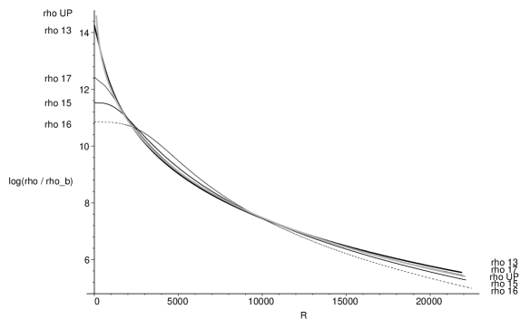
Figure 1: Comparison of density profiles used for Abell clusters. The curves are identified by the numbers given in table LABEL:ACProfileTab. Although each curve is matched to the same pair of $(R,M)$ points (see table LABEL:AbellData), this only ensures the average density within each of those two radii is the same for all profiles, not the actual density.

We considered quite a variety of functional forms for our profiles. For a number of them we fixed the parameters by fitting to the mass-radius data. A comparison of four of these fits with the UP (also fitted to the same data) is shown in figure 1, and in table LABEL:ACProfileTab. Several runs were done with each of these.

——————————

Table LABEL:ACProfileTab goes here

——————————

——————————

Figure 1 goes here

——————————

VII.3.2 A Void

The main feature of a void is a low density region surrounded by walls of higher than background density. Our initial attempt to model a void was to choose a profile with $\rho(M)$ increasing, but this was problematic because we did not have good control over how high the density became before we reached the compensation radius. Thus we designed a profile with a density maximum at the wall, decreasing to background at large $M$. In this way no unreasonable density values are encountered even if the compensation radius is well beyond the density maximum. The profiles tried are summarised in table LABEL:VoidProfileTab and figure 2.

——————————

Table LABEL:VoidProfileTab goes here

——————————

——————————

Figure 2 goes here

——————————

VII.4 Choice of Velocity & Density Profiles at $t_{1}=10^{5}$ yr

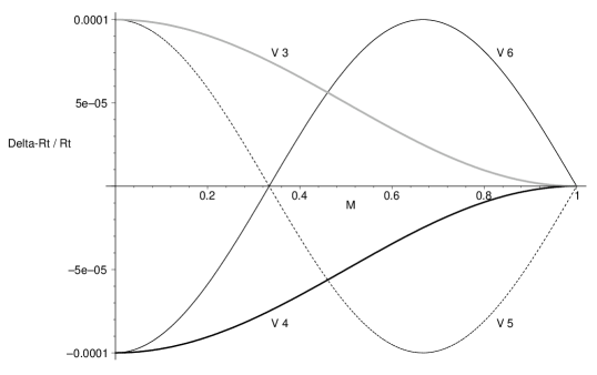
Figure 3: Comparison of initial velocity profiles at recombination. The curves are identified by the numbers given in table LABEL:VelProfileTab.

For velocity fluctuations at recombination, we merely choose a harmonic wave of very low amplitude, with either 1 or 1.5 wavelengths across the diameter of interest. The boundary of the region of interest is the radius that will become the compensation radius at time 2. See table LABEL:VelProfileTab and figure 3 for the details.

——————————

Table LABEL:VelProfileTab goes here

——————————

——————————

Figure 3 goes here

——————————

A few runs were done from initial density profiles, which are given in table LABEL:InFnDenProfileTab.

——————————

Table LABEL:InFnDenProfileTab goes here

——————————

VIII Programs

The foregoing procedure to solve for the L-T functions $E(M)$ and $t_{B}(M)$ from given profiles $R_{,t1}(M)$ and $\rho_{2}(M)$, was coded in a set of Maple MapleURL programs that also re-derived and verified the formulas, and fitted the profiles to the data. The programs to evolve the resulting L-T model and plot the results were written in MATLAB MATLABURL . Unlike the Maple programs, the latter did not need large changes from the Paper I versions, but were in any case refined and made more flexible, and in particular were adjusted to handle times where the big crunch has already happened in parts of the model. Also the density to density solving program (Maple) was modified to handle both $\rho_{1}>\rho_{2}$ and $\rho_{2}\geq\rho_{1}$.

As before, slightly different variables from those used in the foregoing algebra were more convenient for the numerics. In particular, for the velocity to density case, in place of $x$, $a_{2}$, $b_{1}$ and $t_{i}$, we use $y=xa_{2}$, $\beta={b_{1}}^{2}a_{2}$ and $z_{i}=t_{i}/{a_{2}}^{3/2}$. For the velocity to velocity case we use $y=x/{b_{2}}^{2}$, $\gamma={b_{1}}^{2}/{b_{2}}^{2}$ and $z_{i}=t_{i}{b_{2}}^{3}$. Expressions for the following limits at the origin are also needed,

$$\begin{split}a_{i}(0)&=\lim_{M\rightarrow 0}\frac{R(t_{i},M)}{M^{1/3}}=\left(\frac{6}{\kappa\rho(t_{i},0)}\right)^{1/3}\\ &=\frac{2}{{b_{i}}^{2}(0)\mp x(0)},\end{split}$$ (8.1)

$$b_{i}(0)=\lim_{M\rightarrow 0}\frac{R_{,t}(t_{i},M)}{M^{1/3}}=\epsilon\sqrt{\frac{2}{a_{i}(0)}\pm x(0)},$$ (8.2)

where the upper sign is for the hyperbolic case and the lower one for the elliptic case; $\epsilon=+1$ is for expansion, and $\epsilon=-1$ for collapse. Since $x(0)$ comes from the solution procedure, we have an expression for $a_{i}(0)$, whether velocity or density profiles are given, but for $b_{i}(0)$ when the velocity profile is given, the limit must be calculated using the explicit velocity profile function. Alternatively, the velocity may be given in the form $b_{i}(M)$.

For reconstructing the model evolution from the solution functions $x$ and $t_{B}$, the formulas in Paper I still suffice.

IX Runs

The runs that we did are listed in table LABEL:RunList, which also lists the relevant figure numbers where appropriate, and the significance of each run.

——————————

Table LABEL:RunList goes here

——————————

——————————

Run Figures go here

——————————

X Results

A run is defined by specifying one of the initial profiles, $\rho_{1}$ & $R_{,t1}$, and one of the final profiles, $\rho_{2}$ & $R_{,t2}$. The results of a particular run are the two L-T functions $E(M)$ and $t_{B}(M)$ — the local energy/geometry function and the local bang time function — that determine the L-T model. The model so defined may then be evolved over any time range, or its whole lifetime, and in particular, it can be verified that the given profiles are reproduced. In addition, of the 4 profiles $\rho_{1}$, $R_{,t1}$, $\rho_{2}$ and $R_{,t2}$, the two that were not used to define the run are also determined by $\{E(M),t_{B}(M)\}$, and are of interest, especially the initial one.

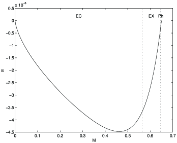
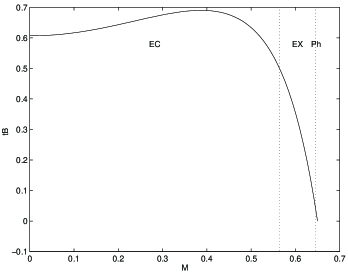
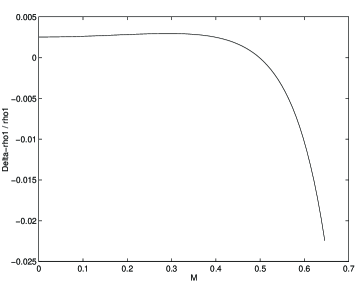
Figure 5: $E(M)$, $t_{B}(M)$ and the $\rho_{1}(M)$ fluctuation for run $V$i4$\rho$f16, in which a region of initially low expansion rate evolves into an Abell cluster. In this and other figures, “H”, “EX”, “EC”, “Pe” and “Ph” indicate regions that are hyperbolic, elliptic and still expanding at time $t_{2}$, elliptic and recollapsing at time $t_{2}$, elliptic but within the range for a series expansion about the parabolic model, and hyperbolic but within the range for a series expansion about the parabolic model.

• The primary Abell cluster forming run, $V$i4$\rho$f16 (fig. 5), used an improved present day density profile based on observational results, and also started from an initial velocity profile that was expanding less fast than the background at the centre, which is what one would expect to evolve into a condensation, see figs. 3 and 5. Though an Abell cluster model was generated in Paper I, the final profile was not so carefully chosen, and it was evolved from an initial density profile. However, the evolution of $\rho$, $R$ and $R_{,t}$ is visually very similar to that given in paper I. The main differences are at $t_{1}$. Several runs with different initial velocity profiles gave quite similar results — with only $\rho_{1}$ and $t_{B}$ changing significantly.

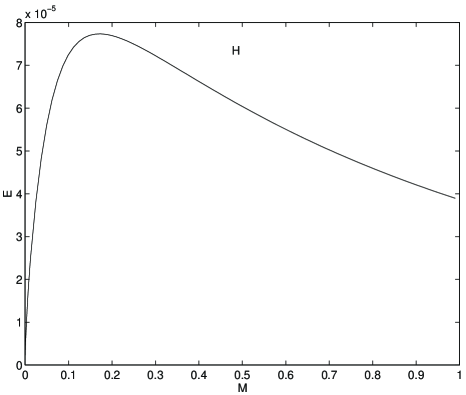
Figure 7: $E(M)$ for run $V$i3$\rho$f20, which successfully creates a present day void. Though shell crossings are inevitable, they don’t occur for a long time after the present.

• The primary void forming run, $V$i3$\rho$f20 (figs. 7, 8, 9, 10), used an initial state that was expanding faster than the background at the centre, which is what one would expect to evolve into a low density region. Using $\rho$f20 for the final density profile was particularly successful, as the required density profile develops smoothly, and the density is still decreasing at every point even at the present time, so there is no sign of imminent shell crossings.

  It is evident from the plots of $E$ & $t_{B}$ and the conditions for no shell crossings HeLa1985 , that there must be shell crossing at some time, but these are long before recombination, and well after the present time. A significant feature is the relatively low central density at the initial time. The evolution of voids in an L-T model has been extensively discussed by Sato and coworkers, see a summary in Ref. Sato1984 . They, too, found that it necessarily leads to a shell crossing at some time.

  Our original attempt, using $\rho$18, created a shell crossing (where the density diverges and then goes negative) so soon after $t_{2}$, that the model evolution program could only generate smooth density profiles up to $0.98t_{2}$.

• The case of a pure density perturbation, $V$i0$\rho$f13, was investigated by choosing a flat initial $b_{1}$ evolving to a cluster. This shows what initial density perturbation is needed at recombination to form the cluster by today — a central overdensity surrounded by an underdensity, of order $10^{-3}$.

  Similarly, the case of a pure velocity perturbation, $\rho$i0$\rho$f13, created by choosing a flat initial $\rho_{1}$ evolving to a cluster, shows what initial velocity perturbation is needed — a general underexpansion of order $10^{-4}$, decreasing outwards.

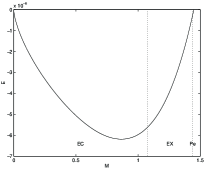
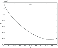
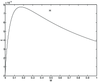
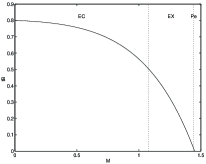
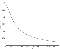
Figure 6: $E(M)$, $t_{B}(M)$ the $\rho_{1}(M)$ or $R_{,t1}(M)$ fluctuation, and the $\rho(t,M)$ evolution (top to bottom) for runs $V$i0$\rho$f13, $\rho$i0$\rho$f13 and $\rho$i0$\rho$f20 (left to right). The left and middle columns show the pure density and pure velocity fluctuations needed at recombination to create an Abell cluster today. The middle and right columns show the difference in the pure velocity fluctuations needed at recombination to create an Abell cluster and a void today.

  The latter is contrasted with the pure velocity perturbation needed to create a void in $\rho$i0$\rho$f20 — a general overexpansion of order $10^{-2}$, decreasing outwards. (See fig. 6 for all 3 runs.)

  The rather large size of these perturbations tends to confirm that perturbations in both density and velocity are needed.

• Our entire approach — specifying profiles for an L-T model at 2 different times — demonstrates that two L-T models with identical $\rho(M)$ [and consequently $R(M)$] at a given time, or identical $R_{,t}(M)$ at a given time, can have quite different evolutions. This is shown by comparing runs $\rho$i0$\rho$f13 & $\rho$i0$\rho$f20 (both in fig 6); also by runs $V$i4$\rho$f16 & $V$i4$\rho$f0; and in a small way by the set of 4 runs that all end with $\rho$f0. Thus, knowledge of only the density (or velocity) profile at one time does not determine a model’s evolution at all.

• To make clearer the effect of varying the initial velocity profiles, a set of runs was done with all 4 initial $V$ profiles and the homogeneous final $\rho$ profile. We found $t_{B}$ has almost the same shape as the velocity perturbation $b_{1}$; $E$ is strongly influenced by $b_{1}$, except that it starts from zero at $M=0$, and returns close to zero at $M=M_{c}$; and the $\rho_{1}$ perturbation is also strongly dictated by $b_{1}$, but turns away from zero towards $M=M_{c}$.

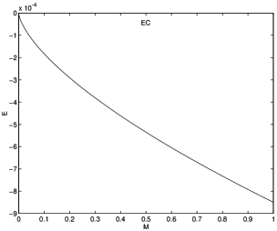
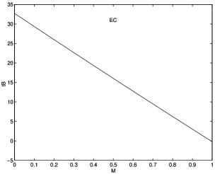
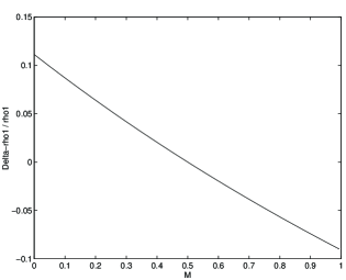
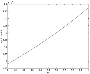
Figure 11: $E(M)$, $t_{B}(M)$ and the $\rho_{1}(M)$ and $\rho_{2}(M)$ fluctuations for run $\rho$i3$\rho$f21. The densities $\rho_{1}$ & $\rho_{2}$ at times $t_{1}$ & $t_{2}$ are of comparable magnitude (which makes $\rho_{2}$ around $2\times 10^{10}$ times the parabolic background at $t_{1}$). In particular, $\rho_{1}>\rho_{2}$ at the centre, $M=0$, and $\rho_{2}>\rho_{1}$ at the edge, $M=1$.

• Run $\rho$i3$\rho$f21 (fig. 11) demonstrates the density profile inversion that MusHel01 proved was not only possible but likely, and our method makes it easy to obtain such evolutions.

  This same run also shows a model can evolve from lower to higher density in one region and higher to lower in another; and that our method can handle such occurrences.

• For the two times we have been considering — $t_{1}$ at recombination and $t_{2}$ at the present day — the shape of the resultant $E(M)$ in any given run is dominated by the final density profile, while both initial and final profiles have a noticeable effect on the resultant $t_{B}(M)$.

• We have found that, when choosing the initial velocity fluctuation with an appropriate magnitude, it is quite difficult to keep the initial density fluctuation (which is not chosen) small enough, and vice-versa. The main run of Paper I, which imposed a final density profile of similar scale to $\rho$f13, but less centrally concentrated, and a $3\times 10^{-5}$ density fluctuation at $t_{1}$, was quite successful in this regard, having a resulting velocity variation that was within $3\times 10^{-5}$ over much of its range, only reaching $8\times 10^{-4}$ in the outer regions that evolved into vacuum. This sensitivity to profile shape, and better way of choosing initial profiles could be investigated further.

• The compensation radius was close to a parabolic point in every run. This must in fact be the case to high approximation under the conditions we imposed. Since we are using a $k=0$ Friedmann model as our reference or background model, then any L-T model which has the same $M$ within the same $R$ at the same $t-t_{B}$ must be locally the same (same $R(t,M_{c})$) as the background, and therefore parabolic. By definition, the compensation radius is where $M$ & $R$ are the same as in the background, but in general our method does not ensure $t-t_{B}$ matches there. At the beginning of the calculation, we do not know $(t-t_{B})$ yet, it is one of the results of the procedure. As explained is sec. IV.4, the individual values of the time coordinate have no meaning. Only the differences, $(t_{2}-t_{1})$, $(t_{2}-t_{B})$, $(t-t_{B})$, etc, appear in the calculations and are physical parameters. Nevertheless, we assume that our $t_{2}$ equals $(t_{2}-t_{B})$ in the background. In consequence, $t_{B}=0$ in the background, while in general $t_{B}(M_{c})\neq 0$ in the perturbation. However, in practice, our use of tiny deviations from the background value at recombination $t_{1}$, ensures that the jump in $t_{B}$ can only be very slight. This is what ensures a close-to-parabolic model at $M_{c}$.

• As a result of the above, in each of the numerical examples $E(M)$ has the same sign in the whole range. However, the method discussed here and in Paper I can be freely applied to models in which $E(M)$ changes sign at some $M$ — see Paper I for an example.

XI Conclusions

• It is traditional to think of spacetimes as being specified by functions such as components of the metric and its derivative, or density and velocity, given on some initial surface. We have taken the new approach of specifying one function on an initial surface and another on a final surface, and demonstrated that, in the case of the L-T model, an evolution from one to the other can be found. This approach is better suited to feeding the observational data into the model functions.

• In particular, the spherically symmetric evolution from a given initial velocity (or density) profile to another given density (or velocity) profile, in any of the four possible combinations, can always be found. The solution is a determination of the arbitrary functions that characterise the model. While there is no guarantee that the resulting model will be free of shell crossings, it is a simple matter to check the arbitrary functions once calculated, and our experience has shown that reasonable choices of the profiles keep any shell crossing well before the initial time or well after the final time.

• The solution method has been programmed, and a variety of runs have demonstrated the practicality of the method. Models of a void and of an Abell cluster have been generated, and shown to have well behaved evolutions between the initial and final times. It is noteworthy that the void model was able to concentrate matter into a wall without the formation of any shell crossings up to the present time and for well after it.

• The effect on the solution of varying the initial and final profiles was effectively illustrated. Some other previously known features of the L-T model, such as the possibility that clumps could evolve into voids, were highlighted in the results section by producing examples.

Appendix A Extensions of Paper I — the evolution between two density profiles.

A.1 Models with Both Larger and Smaller Densities at Later Times

It is clear from the method of Paper I that, for any $r$ value, whatever solution is found for $\rho_{2}<\rho_{1}$, its time reverse ($t\rightarrow t_{1}+t_{2}-t$, $t_{B}\rightarrow t_{1}+t_{2}-t_{B}$) will solve the case when the density values are interchanged. But could both $\rho(t_{1},r_{a})>\rho(t_{2},r_{a})$ and $\rho(t_{1},r_{b})<\rho(t_{2},r_{b})$ occur at different $r$ values $r_{a}$ & $r_{b}$ in the same model? It is obvious that a model with adjacent expanding and collapsing hyperbolic regions must have severe shell crossings, unless they were separated by a neck Hell1987 . But the latter puts the two hyperbolic regions on either side of a wormhole, so they don’t really communicate. On the other hand it seems entirely possible that two worldlines in an elliptic region could display such behaviour, or even a hyperbolic region outside an elliptic region.

In Paper I, the condition $\rho_{2}(M)\leq\rho_{1}(M)$ was imposed merely to ensure $R_{2}\geq R_{1}$, which allowed us to know there was always a bang in the past, and hence a well defined $t_{B}$. However, we note that this condition did not exclude other equally unreasonable possibilities, such as an elliptic region outside a hyperbolic region (see HeLa1985 ).

Thus, if we relax this requirement, and allow all $\rho_{1}>0$ and all $\rho_{2}>0$ profiles, we merely have to note which of $R_{1}$ & $R_{2}$ is larger before generating the ”forwards” or ”backwards” solution.

We in any case have to check whether the conditions for no shell crossings HeLa1985 are satisfied, or whether a regular maximum or minimum has been reached, and this merely adds one more thing to check — whether the bang and crunch functions are sufficiently continuous.

A.2 Including regions of zero density in the profiles

A.2.1 Transient zeros in the density

Given the expression for the density, (2.3) it is clear that if $M_{,r}=0$ for a particular $r$, but $E_{,r}$ and $(t_{B})_{,r}$ are not zero, the density will be zero there for all time. Is it possible that $\rho=0$ at isolated events, or on non-comoving worldsheets?

Assuming $M_{,r}\neq 0$ and $0<R<\infty$, the only way for this to happen would be for $R_{,r}$ to diverge without changing sign, while $M_{,r}$ remains finite. We immediately see that divergent $R_{,r}$ makes $g_{rr}$ divergent, which suggests bad coordinates at the very least. However, for all $E$ values we may write HelLak84 ; Barn1970

$$\begin{split}\frac{R_{,r}}{R}=&\left(\frac{M_{,r}}{M}-\frac{E_{,r}}{E}\right)R\\ &-\left[(t_{B})_{,r}+\left(\frac{M_{,r}}{M}-\frac{3E_{,r}}{2E}\right)(t-t_{B})\right]R_{,t}\end{split}$$ (A.1)

and it is clear that $t_{B,r}R_{,t}$ is only divergent on the bang or crunch, while $(t-t_{B})R_{,t}$ is zero there, because $R_{,t}\sim(t-t_{B})^{-1/3}$ at early times. So one possibility is that $t_{1}$ intersects a non-simultaneous bang while $t_{2}$ does not intersect the crunch at the same $r$ value, or vice versa. This of course means the constant time surface cannot be extended beyond this point, which is not really satisfactory. The only other possibility is for $E_{,r}$ or $t_{B,r}$ to diverge.But this would give a comoving zero of density, and a coordinate transformation would make $E_{,r}$ and/or $t_{B,r}$ finite and $M_{,r}$ zero.

Thus we conclude that, apart from the case of the initial or final surface intersecting the bang or crunch, the density along a particle worldline cannot be zero at one time and non-zero at another. Thus zeros of density have to be permanent and comoving.

A.2.2 $\rho(M)=0$ at a single $M$ value

To look at the question of whether zero density at a single $M$ value can be accommodated in the methods of Paper I, we first determine what kind of zero we might expect in $\rho(M)$. Working in flat 3-d space, let

$$\rho(R)\approx A|R-R_{z}|^{n},~{}~{}~{}~{}~{}~{}~{}~{}A,n\text{ const \&}>0$$ (A.2)

near a zero in $\rho$. Then

$$|M-M_{z}| = 4\pi\int_{R_{z}}^{R}\rho(R^{\prime}){R^{\prime}}^{2}\,dR^{\prime}$$ (A.3)

$$= 4\pi A\left(\frac{|R-R_{z}|^{n+3}}{n+3}+\frac{2R_{z}|R-R_{z}|^{n+2}}{n+2}\right.$$

$$+\left.\frac{R_{z}^{2}|R-R_{z}|^{n+1}}{n+1}\right),$$

so, to lowest order

$$|M-M_{z}| \approx 4\pi A\,\frac{R_{z}^{2}\,|R-R_{z}|^{n+1}}{n+1},$$ (A.4)

$$|R-R_{z}| \approx \left(\frac{(n+1)|M-M_{z}|}{4\pi AR_{z}^{2}}\right)^{1/(n+1)},$$ (A.5)

which means

$$\rho(M)\approx A\left(\frac{(n+1)|M-M_{z}|}{4\pi AR_{z}^{2}}\right)^{n/(n+1)},$$ (A.6)

and we notice $n/(n+1)<1$ always.

If we use this as an approximation near a point zero in the full curved spacetime expression, we find

$$\begin{split}R^{3}-R_{z}^{3}&=\int_{M_{z}}^{M}\frac{6}{\kappa\rho(M^{\prime})}\,dM^{\prime}\\ &=\frac{6}{\kappa B}(n+1)|M-M_{z}|^{1/(n+1)},\end{split}$$ (A.7)

which is indeed well determined. We thus conclude that no modification of the Paper I method is needed in principle, though some extra coding might be needed if the integration had to be done numerically. (With all the profiles tried so far, Maple did symbolic integrations to get $R_{i}^{3}$.)

A.2.3 $\rho=0$ over an extended region

We have already seen that zeros in the density have to be permanent and comoving, and this obviously applies to extended vacuum regions. In any case, spherically symmetric vacuum is Schwarzschild and must remain so.

In order to allow the possibility that $\rho(t_{i},r)$ is zero over a finite range, the choice $\rho_{i}=\rho_{i}(M)$ must be abandoned as all points in the zero density region will have the same mass, so $M$ will be a degenerate coordinate there.

Whatever alternative possibilities we choose must allow us to identify the corresponding comoving coordinate points on each of the density profiles at $t_{1}$ & $t_{2}$. Thus $R$ is not a suitable coordinate, as the two $R(t_{i},r)$ are different.

Thus we instead consider the following alternatives:

1. Specify $\rho_{i}=\rho_{i}(r)$ and $M=M(r)$
   This parametric version of choosing $\rho(M)$, allows $\rho_{i}(r)=0$ and $M(r)=const$ over some range of $r$, but actually is not sufficient, as we still have no idea how much $R_{i}(r)$ increases over this range — how much space there is between the non-vacuum regions. In other words, in such a range, neither $\rho_{i}(r)$ nor $M(r)$ provides a useable definition of $r$ in terms of a physical quantity.

2. Specify $\rho_{i}=\rho_{i}(R_{i})$
   in which case

   $$M_{i}(R)=(\kappa/2)\int_{0}^{R}R_{i}^{2}\rho_{i}(R)dR.$$ (A.8)

   Now where $\rho_{i}>0$, $M(R)$ will be different for each $R$ value, and therefore can be used to identify corresponding points on the two profiles. We can then use $R_{2}$ or $R_{1}$ (or something else) as the coordinate radius $r$. Let us say we choose $r=R_{2}$. But for regions where $\rho_{i}=0$, $M(R)$ will be degenerate. In this case, we take advantage of the fact that in vacuum there are no matter particles, and so we have extra freedom in choosing the geodesics that constitute our constant $r$ paths. Using a linear interpolation between the $R$ values at the two edges of the vacuum region at each of $t_{1}$ & $t_{2}$ provides the obvious choice of corresponding points, i.e. at time $t_{2}$,

   $$r=R_{2},$$ (A.9)

   and at time $t_{1}$,

   $$r=\left\{\begin{array}[]{ll}R_{2,\text{vac,min}}+\frac{(R_{1,\text{vac}}-R_{1,\text{vac,min}})(R_{2,\text{vac,max}}-R_{2,\text{vac,min}})}{(R_{1,\text{vac,max}}-R_{1,\text{vac,min}})}&\text{~{}~{}in vacuum,}\\ M_{2}^{-1}(M_{1}(R_{1}))&\text{~{}~{}in non-vacuum.}\end{array}\right.$$ (A.10)

   The original procedure for extracting the functions $E$ and $t_{B}$, which actually used $R_{1}$ & $R_{2}$, goes through with the only change that functions of $r=M$ are now functions of $r=R_{2}$. In particular, in vacuum regions, each worldline has different pairs of $R_{1}$ & $R_{2}$ values, but the same $M$ value.

Appendix B The evolution of $R(t,M)$ vs the evolution of $\rho(t,M)$.

Let us take the relation between $R$ and $\rho$ in the most general case, without any assumptions, eq. (2.10).

This means that the value of $R$ at any $M$ depends on the values of $\rho$ in the whole range $[M_{0},M]$. Also the inverse relation, (2.9), is nonlocal — to find $\rho(t,M)$ we need to know $R$ in an open neighbourhood of the value of $M$.

Assume now $\rho_{2}<\rho_{1}$ over the whole of $[M_{0},M]$. Then

$$\begin{split}&R_{2}^{3}(M)-R_{1}^{3}(M)-\left({R_{0}}^{3}(t_{2})-{R_{0}}^{3}(t_{1})\right)\\ &=\frac{6}{\kappa}\int^{M}_{M_{0}}\left(\frac{1}{\rho_{2}(u)}-\frac{1}{\rho_{1}(u)}\right)\text{d}u>0.\end{split}$$ (B.1)

Hence, $R_{2}^{3}(M)>R_{1}^{3}(M)$ if

$${R_{0}}^{3}(t_{2})-{R_{0}}^{3}(t_{1})+\frac{6}{\kappa}\int^{M}_{M_{0}}\left(\frac{1}{\rho_{2}(u)}-\frac{1}{\rho_{1}(u)}\right)\text{d}u>0.$$

This will hold if we assume, as was done in paper I, $R_{0}(t_{i})=0,i=1,2$ in addition to $\rho_{2}<\rho_{1}$. The assumption $M_{0}=0$, i.e. the absence of a mass-point at $R=0$, also made in paper I, is not needed for this purpose.

The converse implication is simply not true: $R(t_{2},M)>R(t_{1},M)$ for all $M\in[M_{0},M_{1}]$ does not imply anything for the relation between $\rho(t_{2},M)$ and $\rho(t_{1},M)$. This somewhat surprising fact is easy to understand on physical grounds. $R(t_{2},M)>R(t_{1},M)$ for all $M\in[M_{0},M_{1}]$ means that every shell of constant $M=\tilde{M}$ has a larger radius at $t_{2}$ than it had at $t_{1}$. However, the neighbouring shells may have moved closer to $\tilde{M}$ at $t_{2}$ than they were at $t_{1}$. If they did, then a local condensation around $\tilde{M}$ was created that may result in $\rho(t_{2},\tilde{M})$ being larger than $\rho(t_{1},\tilde{M})$. This does not happen in the Friedmann limit, where local condensations are excluded by the symmetry assumptions.

A sufficient condition for $\rho_{2}(M)<\rho_{1}(M),M\in[M_{0},M_{1}]$ is

$$\frac{1}{\left({R_{1}}^{3}\right),_{M}}>\frac{1}{\left({R_{2}}^{3}\right),_{M}}\qquad\text{for all }M\in[M_{0},M_{1}].$$

If $R,_{M}>0$ for all $M\in[M_{0},M_{1}]$ at both $t_{1}$ and $t_{2}$ (i.e. there are no shell-crossings in $[M_{0},M_{1}]$), then this is equivalent to ${\left({R_{2}}^{3}\right),_{M}}>{\left({R_{1}}^{3}\right),_{M}}$ for all $M\in[M_{0},M_{1}]$. Incidentally, this implies $R_{2}>R_{1}$ for all $M\in[M_{0},M_{1}]$ if $R_{2}(M_{0})>R_{1}(M_{0})$.

Appendix C Calculations for section IV.

C.1 Derivation of (4.33) and (4.34).

In eq. (4.31) we have

$$\Phi_{X}(0) =0,$$

$$\Phi_{X}\left(2/a_{2}\right)= \pi+\frac{b_{1}\sqrt{2a_{2}}}{a_{2}{b_{1}}^{2}/2+1}-\arccos\left(\frac{a_{2}{b_{1}}^{2}/2-1}{a_{2}{b_{1}}^{2}/2+1}\right)$$

$$-\left(2/a_{2}\right)^{3/2}\left(t_{2}-t_{1}\right),$$ (C.1)

$$\begin{split}\Phi_{X,x}&=\sqrt{x}\left[\frac{{a_{2}}^{3/2}}{\sqrt{2-a_{2}x}}-\frac{2b_{1}}{\left({b_{1}}^{2}+x\right)^{2}}-\frac{3}{2}\left(t_{2}-t_{1}\right)\right]\\ &:=\sqrt{x}\lambda_{X}(x).\end{split}$$ (C.2)

We see that $\Phi_{X,x}(0)=0$ and that $\lim_{x\to 2/a_{2}}\Phi_{X,x}=+\infty$. Now $\lambda_{X,x}(x)=\frac{1}{2}{a_{2}}^{5/2}/(2-a_{2}x)^{3/2}+4b_{1}/({b_{1}}^{2}+x)^{3}>0$ for all $x\in[0,2/a_{2}]$. Hence, $\lambda_{X}$ can have at most one zero and it will have one only if $\lambda_{X}(0)<0$, i.e. if eq. (4.33) holds.

With (4.33) fulfilled, $\Phi_{X,x}<0$ in a neighbourhood of $x=0$, $\Phi_{X,x}=0$ at some $x=x_{\text{min}}$, and $\Phi_{X,x}\to+\infty$ at $x\to 2/a_{2}$; the latter means that the tangent to $\Phi_{X}(x)$ at $x=2/a_{2}$ is vertical. Consequently, $\Phi_{X}(x)$ itself is a decreasing function for $x\in[0,x_{\text{min}})$, and is negative in this range, then it is increasing for $x\in(x_{\text{min}},2/a_{2}]$. It can thus have a zero at any $x>0$ if and only if $\Phi_{X}(2/a_{2})\geq 0$, i.e. if (4.34) is fulfilled.

C.2 Derivation of (4.40).

The relevant properties of $\Phi_{C}(x)$ are

$$\Phi_{C}(0) =2\pi>0,$$

$$\Phi_{C}(2/a_{2})= \pi+\frac{b_{1}\sqrt{2a_{2}}}{a_{2}{b_{1}}^{2}/2+1}-\arccos\left(\frac{a_{2}{b_{1}}^{2}/2-1}{a_{2}{b_{1}}^{2}/2+1}\right)$$

$$-\left(2/a_{2}\right)^{3/2}\left(t_{2}-t_{1}\right),$$ (C.3)

$$\begin{split}\Phi_{C,x}(x)&=-\sqrt{x}\left[\frac{{a_{2}}^{3/2}}{\sqrt{2-a_{2}x}}+\frac{2b_{1}}{\left({b_{1}}^{2}+x\right)^{2}}+\frac{3}{2}\left(t_{2}-t_{1}\right)\right]\\ &<0.\end{split}$$ (C.4)

Since $\Phi_{C}(0)>0$ and $\Phi_{C,x}<0$ for all $x>0$, the function $\Phi_{C}(x)$ may have (only one) zero anywhere in its range if and only if $\Phi_{C}(2/a_{2})\leq 0$, which translates into the opposite of (4.34), i.e. eq. (4.40).

Appendix D The velocity at $t_{2}$ must be smaller than at $t_{1}$ in the hyperbolic evolution.

We now show that ${b_{1}}^{2}>{b_{2}}^{2}$ must hold, as stated in subsection V.1.1, in consequence of $t_{2}>t_{1}$ and $\left.R_{,t}\right|_{t=t_{1}}>0$, i.e. $b_{1}>0$. (The assumption $R_{,t}(t_{1})>0$ is hidden already in eqs. (2.4) – (2.6); for $R_{,t}<0$, $(t-t_{B})$ would have to be replaced by $(t_{B}-t)$ in all three places.)

Suppose that ${b_{2}}^{2}>{b_{1}}^{2}$, so that $x<{b_{1}}^{2}$ applies. Then

$$\lim_{x\to{b_{1}}^{2}}\chi_{H}(x)=-\infty,$$ (D.1)

and in addition $\chi_{H}(0)=0$ (this second property does not depend on the sign of ${b_{2}}^{2}-{b_{1}}^{2}$). It follows that a second zero of $\chi_{H}(x)$ will exist if there exists a subset of $R^{1}_{+}$ on which $\chi_{H}$ is an increasing function. From Eq. (5.6) we see that $\chi_{H,x}(0)=0$, $\lim_{x\to{b_{1}}^{2}}\chi_{H,x}=-\infty$. Hence, in order that $\chi_{H}(x)$ may have a zero at $x>0$, the $\mu_{H}(x)$, defined in (5.6), must be positive somewhere in the range $x>0$. The derivative of $\mu_{H}(x)$ is

$$\mu^{\prime}_{H}(x)=\frac{4b_{2}}{\left({b_{2}}^{2}-x\right)^{3}}-\frac{4b_{1}}{\left({b_{1}}^{2}-x\right)^{3}},$$ (D.2)

and so there must exist values of $x$ such that

$$b_{2}\left({b_{1}}^{2}-x\right)^{3}-b_{1}\left({b_{2}}^{2}-x\right)^{3}>0.$$ (D.3)

This is equivalent to

$$\left[\left(b_{1}/b_{2}\right)^{1/3}-1\right]x>{b_{1}}^{1/3}\left({b_{2}}^{5/3}-{b_{1}}^{5/3}\right).$$ (D.4)

However, this is a contradiction since, with $b_{1}<b_{2}$ and $x>0$, the left-hand side is negative, and the right-hand side is positive.

Since ${b_{2}}^{2}>{b_{1}}^{2}$ has thus led to a contradiction, the opposite must hold. This result is intuitively obvious (for dust, expansion must slow down with time), so the above is in fact just a consistency check.

Appendix E The velocity at $t_{2}$ must be smaller than at $t_{1}$ in the elliptic evolution (final state still expanding).

We will prove here that the $b_{2}$ in eq. (5.13) must be smaller than $b_{1}$ if, as was assumed earlier, $b_{1}>0$ and $t_{2}>t_{1}$. The proof comes out quite simply if we look at the function $\chi_{X}(x)$ defined by (5.13) as a function of the argument $b_{2}$. At $b_{2}=b_{1}$ we have:

$$\chi_{X}(x)=\chi_{1}(x)=-x^{3/2}\left(t_{2}-t_{1}\right),$$ (E.1)

which is obviously negative for all values of $x>0$. At $b_{2}\to\infty$ we have

$$\begin{split}&\chi_{X}(x)=\chi_{2}(x)=\\ &\sqrt{1-\left(\frac{{b_{1}}^{2}-x}{{b_{1}}^{2}+x}\right)^{2}}-\arccos\left(\frac{{b_{1}}^{2}-x}{{b_{1}}^{2}+x}\right)-x^{3/2}\left(t_{2}-t_{1}\right).\end{split}$$ (E.2)

We find that $\chi_{2}(0)=0$, $\lim_{x\to\infty}\chi_{2}(x)=-\infty$ and the derivative is $\chi^{\prime}_{2}(x)=-2b_{1}\sqrt{x}/({b_{1}}^{2}+x^{2})^{2}-(3/2)\sqrt{x}(t_{2}-t_{1})$ — obviously negative for all $x>0$. Therefore $\chi_{2}(x)$ itself is negative for all $x>0$.

Now we calculate:

$$\frac{\partial\chi_{X}(x)}{\partial b_{2}}=-\frac{4x^{3/2}}{\left({b_{2}}^{2}+x\right)^{2}},$$ (E.3)

which is negative for all values of $b_{2}$ at every value of $x>0$. Thus, $\chi_{X}(x)$ is negative for all $x>0$ at $b_{2}=b_{1}$, negative for all $x>0$ at $b_{2}\to\infty$ and is a decreasing function of $b_{2}$ at every $b_{2}\in(b_{1},\infty)$ for every $x>0$. This means that $\chi_{X}(x)$ is negative at every value of $x>0$ for any $b_{2}>b_{1}$, and so the equation $\chi_{X}(x)=0$ has no solutions in $(0,\infty)$ when $b_{2}>b_{1}$.    o   

Appendix F Tables

Table 1: Geometrical Units. The sets of geometrical units used for models of Abell clusters and for of voids.

Object	$M_{G}$	$L_{G}$	$T_{G}$
Abell clusters	$10^{15}~{}M_{\odot}$	$47.84$ parsecs	$156.0$ years
Voids	$55\times 10^{15}~{}M_{\odot}$	$2631$ parsecs	$8582$ years

Table 2: Abell Cluster Data. Data from MVFS1999 , giving the observed masses within 0.2 Mpc and 1 Mpc deduced from X-ray observations, which is used to fit the profiles in table LABEL:ACProfileTab to observations.

Abell Cluster	$M$(0.2 Mpc)	$M$(1 Mpc)
A 2199	$(0.65\pm 0.11)\times 10^{14}~{}M_{\odot}$	$(2.9\pm 0.3)\times 10^{14}~{}M_{\odot}$
A 496	$(0.47\pm 0.10)\times 10^{14}~{}M_{\odot}$	$(3.1\pm 0.3)\times 10^{14}~{}M_{\odot}$

Table 3: Abell cluster profiles. The equations and properties of the profiles shown in fig 1, that were used to model the present density distribution in Abell clusters. The parameters given are those that fit the A2199 data MVFS1999 . All non-dimensionless values are in geometric units — see table LABEL:GeomU.

Profile	$\rho/\rho_{b}$	Parameters	$R_{c}$	$M_{c}$
$\rho$fUP	$\frac{\rho}{\rho_{b}}=\frac{\delta}{\frac{R}{R_{s}}\left(1+\frac{R}{R_{s}}\right)^{2}}$	$\delta=77440$, $R_{s}=3457~{}L_{G}$	$324600~{}L_{G}$	$0.9442~{}M_{G}$
$\rho$f13	$\frac{\rho}{\rho_{b}}=\frac{B_{2}e^{-\sqrt{M}\;/\sigma_{2}}}{\left(\nu_{2}+\frac{\sqrt{M}\;}{\mu_{2}}\right)\left(1+\frac{\sqrt{M}\;}{\mu_{2}}\right)}$	$B_{2}=7774000$, $\mu_{2}=0.05304~{}\sqrt{M_{G}}\;$, $\sigma_{2}=2\mu_{2}$, $\nu_{2}=5$	$374500~{}L_{G}$	$1.449~{}M_{G}$
$\rho$f15	$\frac{\rho}{\rho_{b}}=\frac{B_{2}e^{-M/\sigma_{2}}}{\left(\nu_{2}+\frac{M}{\mu_{2}}\right)\left(1+\frac{M}{\mu_{2}}\right)}$	$B_{2}=507500$, $\mu_{2}=0.04474~{}M_{G}$, $\sigma_{2}=2\mu_{2}$, $\nu_{2}=5$	$312400~{}L_{G}$	$0.8416~{}M_{G}$
$\rho$f16	$\frac{\rho}{\rho_{b}}=\frac{B_{2}}{1+e^{M/\mu_{2}}}$	$B_{2}=103400$, $\mu_{2}=0.04577~{}\sqrt{M_{G}}\;$	$286600~{}L_{G}$	$0.6500~{}M_{G}$
$\rho$f17	$\frac{\rho}{\rho_{b}}=\frac{B_{2}}{1+e^{\sqrt{M}\;/\mu_{2}}}$	$B_{2}=498500$, $\mu_{2}=0.07144~{}M_{G}$	$349800~{}L_{G}$	$1.182~{}M_{G}$

Table 4: Void Profiles. The equations and properties of the profiles shown in fig 2, that were used to model the present density distribution in voids. The parameters were chosen to give a low density region well below the background value (see $[\rho/\rho_{b}]_{0}$) within 60 Mpc radius. All non-dimensionless values are in geometric units — see table LABEL:GeomU.

Profile	$\rho/\rho_{b}$	Parameters	$[\rho/\rho_{b}]_{0}$	$R_{c}$	$M_{c}$
$\rho$f18	$\frac{\rho}{\rho_{b}}=A_{2}+B_{2}e^{M/\mu_{2}}$	$A_{2}=0.01$, $B_{2}=0.01$, $\mu_{2}=0.01429~{}M_{G}$,	0.01	$22804~{}L_{G}$	$0.9902~{}M_{G}$
$\rho$f20	$\frac{\rho}{\rho_{b}}=\frac{B_{2}^{2}\mu_{2}^{2}+M^{2}}{C_{2}\mu_{2}^{2}+(M-\mu_{2})^{2}}$	$B_{2}=0.3873$, $C_{2}=1$, $\mu_{2}=0.2475~{}M_{G}$,	0.075	$35850~{}L_{G}$	$3.846~{}M_{G}$

Table 5: Initial Velocity Profiles. The equations and properties of the profiles shown in fig 3, that were used to model the initial velocity fluctuations at recombination. The values of $M_{c}$ were determined by the final density profile being used in each run. All values are dimensionless.

Profile	$R_{,t}/(R_{,t})_{b}$	Parameters
$V$i0	$\frac{R_{,t}}{(R_{,t})_{b}}=1$
$V$i3	$\frac{R_{,t}}{(R_{,t})_{b}}=1+A_{1}\left(1+\cos\left(\frac{\pi M}{M_{c}}\right)\right)$	$A_{1}=5\times 10^{-5}$, $M_{c}$ from $t_{2}$ data,
$V$i4	$\frac{R_{,t}}{(R_{,t})_{b}}=1-A_{1}\left(1+\cos\left(\frac{\pi M}{M_{c}}\right)\right)$	$A_{1}=5\times 10^{-5}$, $M_{c}$ from $t_{2}$ data,
$V$i5	$\frac{R_{,t}}{(R_{,t})_{b}}=1+A_{1}\cos\left(\frac{3\pi M}{2M_{c}}\right)$	$A_{1}=1\times 10^{-4}$, $M_{c}$ from $t_{2}$ data,
$V$i6	$\frac{R_{,t}}{(R_{,t})_{b}}=1-A_{1}\cos\left(\frac{3\pi M}{2M_{c}}\right)$	$A_{1}=1\times 10^{-4}$, $M_{c}$ from $t_{2}$ data,

Table 6: Initial and Final Density Profiles. The equations and properties of the profiles that were used to model the initial density fluctuations at recombination and the final structure.

Pro-
file	$\rho/\rho_{b}$	Parameters	Description
$\rho$f0	$\rho/\rho_{b}=1$		Uniform background density at time 2.
$\rho$i0	$\rho/\rho_{b}=1$		Uniform background density at time 1.
$\rho$i3	$\rho/\rho_{b}=\frac{1}{1-A_{1}(1-2M/\mu_{1})}$	$A_{1}=0.1$, $\mu_{1}=1$.	Central overdensity plus surrounding underdensity of order $10^{-1}$ in region of mass $10^{15}M_{\odot}$. Used for the initial profile in run $\rho$i3$\rho$f21.
$\rho$i4	$\rho/\rho_{b}=$ $\left\{\begin{array}[]{lr}\lx@intercol 1+A_{1}\left(1+\cos\left(\frac{100\pi M}{M_{c}}\right)\right),{}{}{}\hfil\lx@intercol\\ &M<\frac{M_{c}}{100}\\ 1,&M\geq\frac{M_{c}}{100}\end{array}\right.$	$A_{1}=1.5\times 10^{-5}$,	Overdensity of order $3\times 10^{-5}$ in region of mass $10^{13}M_{\odot}$, with exactly background density outside it.
$\rho$f21	$\rho/\rho_{b}=\frac{1}{1+A_{2}(1-2M/\mu_{2})}\frac{\rho_{b1}}{\rho_{b2}}$	$A_{2}=0.1$, $\mu_{2}=1$.	Central underdensity plus surrounding overdensity of order $10^{-1}$ in region of mass $10^{15}M_{\odot}$, with a ‘background’ density equal to that at time $t_{1}$. Used for the final profile in run $\rho$i3$\rho$f21.

Table 7: Modelling Runs.

Initial	Final		Function (Fig
profile	profile	Description	no) list	What it shows
$\rho$i4	$\rho$f17	small localised density perturbation $\rightarrow$ Abell cluster	$E(M)$ (4), $t_{B}(M)$ (4), $R_{,t1}(M)$ (4), $\rho(t,M)$ (4),	Classic evolution of a small initial fluctuation with 100th final mass into a condensation with realistic density profile at $t_{2}$.
$V$i4	$\rho$f16	Low central initial expansion rate $\rightarrow$ Abell cluster	$E(M)$ (5), $t_{B}(M)$ (5), $\rho_{1}(M)$ (5)	Evolution of low expansion region, to a realistic density profile at $t_{2}$. Graphs fairly similar to Paper I model.
$V$i0	$\rho$f13	Uniform initial expansion rate $\rightarrow$ Abell cluster	$E(M)$(6, left), $t_{B}(M)$(6, left), $\rho_{1}(M)$(6, left), $\rho(t,M)$(6, left),	Case of a pure density perturbation — how big a perturbation is needed for a present day structure?
$\rho$i0	$\rho$f13	Uniform initial density $\rightarrow$ Abell cluster	$E(M)$(6, centre), $t_{B}(M)$(6, centre), $R_{,t1}(M)$(6, centre), $\rho(t,M)$(6, centre),	Case of a pure velocity perturbation — how big a perturbation is needed for a present day structure?
$\rho$i0	$\rho$f20	Uniform initial density $\rightarrow$ Void	$E(M)$(6, right), $t_{B}(M)$(6, right), $R_{,t1}(M)$(6, right), $\rho(t,M)$(6, right),	Together with $\rho$i0$\rho$f13, shows two models with the same density profile at one time can have totally different evolutions.
$V$i3	$\rho$f18	High central initial expansion rate $\rightarrow$ Void	(None)	Not so good example of evolution to a void — it is so close to a shell crossing at $t_{2}$ that the evolution program fails on the last time step.
$V$i3	$\rho$f20	High central initial expansion rate $\rightarrow$ Void	$E(M)$ (7), $t_{B}(M)$ (8), $\rho_{1}(M)$ (9), $\rho(t,M)$ (10),	Example of evolution to a void with good behaviour at $t_{2}$ and well past it. The density perturbation at $t_{1}$ is too large by 4 orders.
$V$i3	$\rho$f0	High central initial expansion rate $\rightarrow$ Uniform density	(None)	These 4 show very clearly the effect on $E(M)$ & $t_{B}(M)$ of varying initial density
$V$i4	$\rho$f0	Low central initial expansion rate $\rightarrow$ Uniform density		or initial velocity. Since the final density is uniform, the deviation of $E(M)$ &
$V$i5	$\rho$f0	High central & low outer initial expansion rate $\rightarrow$ Uniform density		$t_{B}(M)$ from their FLRW forms is entirely due to non-uniform initial profiles.
$V$i6	$\rho$f0	Low central & high outer initial expansion rate $\rightarrow$ Uniform density		They also show a given density profile at one moment can have many different evolutions.
$\rho$i3	$\rho$f21	Expanding underdensity $\rightarrow$ collapsing overdensity	$E(M)$ (11), $t_{B}(M)$ (11), $\rho_{1}(M)$ (11), $\rho_{2}(M)$ (11),	An example of $\rho_{2}<\rho_{1}$ and within the same model $\rho_{1}<\rho_{2}$. It also provides an example of density profile inversion.

Appendix G Figures

Figure 2: Comparison of density profiles used for voids. The curves are identified by the numbers given in table LABEL:VoidProfileTab.

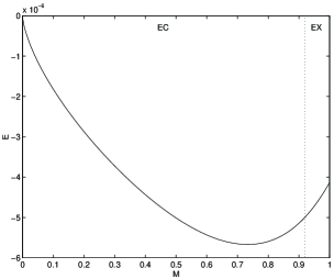
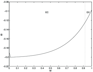
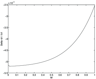
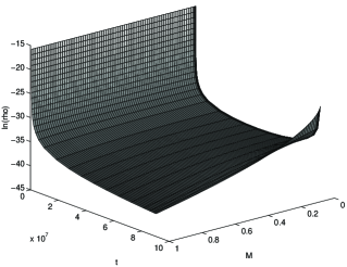
Figure 4: $E(M)$, $t_{B}(M)$, the $R_{,t1}(M)$ fluctuation, and the $\rho(t,M)$ evolution for run $\rho$i4$\rho$f17. Notice the effect of the central bump in $\rho_{1}(M)$ shows up in the $t_{B}$ and $R_{,t1}$ curves. Although $dt_{B}/dM>0$ indicates there will be a shell crossing, the small magnitude of $t_{B}$ ensures it will occur long before $t_{1}$, when the model first becomes valid.

Figure 8: $t_{B}(M)$ for the void run $V$i3$\rho$f20.

Figure 9: $\rho_{1}(M)$ fluctuation for the void run $V$i3$\rho$f20. The amplitude of this fluctuation is too large, so the initial velocity profiles need fine-tuninng.

Figure 10: $\rho(t,M)$ evolution for the void run $V$i3$\rho$f20. Note that $\rho_{2}(M)$ is the same profile as $\rho_{2}(R)$ shown in figure 2, though it looks quite different. The reason is that there is very little mass in the void interior, so a large increase in distance corresponds to a small increase in mass.