Implementation of Time-Delay Interferometry for LISA

Abstract

We discuss the baseline optical configuration for the Laser Interferometer Space Antenna (LISA) mission, in which the lasers are not free-running, but rather one of them is used as the main frequency reference generator (the master) and the remaining five as slaves, these being phase-locked to the master (the master-slave configuration). Under the condition that the frequency fluctuations due to the optical transponders can be made negligible with respect to the secondary LISA noise sources (mainly proof-mass and shot noises), we show that the entire space of interferometric combinations LISA can generate when operated with six independent lasers (the one-way method) can also be constructed with the master-slave system design. The corresponding hardware trade-off analysis for these two optical designs is presented, which indicates that the two sets of systems needed for implementing the one-way method, and the master-slave configuration, are essentially identical. Either operational mode could therefore be implemented without major implications on the hardware configuration.

We then derive the required accuracies of armlength knowledge, time synchronization of the onboard clocks, sampling times and time-shifts needed for effectively implementing Time-Delay Interferometry for LISA. We find that an armlength accuracy of about $16$ meters, a synchronization accuracy of about $50$ ns, and the time jitter due to a presently existing space qualified clock will allow the suppression of the frequency fluctuations of the lasers below to the level identified by the secondary noise sources. A new procedure for sampling the data in such a way to avoid the problem of having time shifts that are not integer multiples of the sampling time is also introduced, addressing one of the concerns about the implementation of Time-Delay Interferometry.

I Introduction

LISA, the Laser Interferometer Space Antenna, is a three-spacecraft deep space mission, jointly proposed to the National Aeronautics and Space Administration (NASA) and the European Space Agency (ESA). The LISA scientific objective is to detect and study low-frequency cosmic gravitational radiation by observing phase differences of laser beams interchanged between drag-free spacecraft 1 .

Modeling each spacecraft with two optical benches, carrying independent lasers, frequency generators (called Ultra Stable Oscillators), beam splitters and photo receivers, the measured eighteen time series of frequency shifts (six obtained from the six one-way laser beams between spacecraft pairs, six from the beams between the two optical benches on each of the three spacecraft, and six more from modulation of the laser beams with USO data) were previously analyzed by Tinto et al. 2 . There it was shown that there exist several combinations of these eighteen observables which exactly cancel the otherwise overwhelming phase noise of the lasers, the phase fluctuations due to the non-inertial motions of the six optical benches, and the phase fluctuations introduced by the three Ultra Stable Oscillators into the heterodyned measurements, while leaving effects due to passing gravitational waves.

The analysis presented in 2 relied on the assumptions that (i) the frequency offsets of any pair of independent lasers (assumed there to be $\approx\ 300\ {\rm MHz}$) could be observed within the detection bandwidths of the photo receivers where the one-way Doppler measurements are performed, and (ii) the telemetry data rate needed by two of the three spacecraft to transmit their measured one-way Doppler data to the third spacecraft (where the interferometric combinations are synthesized) is adequate. Although the technology LISA will be able to use should make possible the implementation of Time-Delay Interferometry (TDI) as discussed in 2 , the possibility of optimizing the design of the optical layout, while at the same time minimizing the number of Doppler data needed for constructing the entire space of interferometric observables, was not analyzed there. Here we extend those results to a different optical configuration, in which one of the six lasers is the provider of the frequency reference (albeit time-delayed) for the other five via phase-locking. This master-slave optical design could provide potential advantages, such as smaller frequency offsets between beams from pairs of different lasers, hardware redundancy, reliability, and can result in a smaller number of measured data. An outline of the paper is given below.

In Section II we summarize TDI, the data processing technique needed for removing the frequency fluctuations of the six lasers used by LISA, and other noises. In order to show that the entire space of interferometric observables LISA can generate can also be reconstructed by using a master-slave optical configuration, we consider the simple case of spacecraft that are stationary with respect to each other. After showing that the entire space of interferometric observables can be obtained by properly combining four generators, ($\alpha,\beta,\gamma,\zeta$), we then derive the expressions for the four generators corresponding to the master-slave optical configuration. By imposing some of the one-way measurements entering into ($\alpha,\beta,\gamma,\zeta$) to be zero (the so called locking conditions), we show that the expressions for these generators can be written in terms of the one-way and two-way Doppler measurements corresponding to the locking configuration we analyzed. Section III and Appendix A provide a theoretical derivation and estimation of the magnitude of the phase noise expected to be generated by an optical transponder. In Section IV we analyze and compare the hardware requirements needed for implementing both optical designs, while in Section V we turn to the estimation of the armlength and time synchronization accuracies, as well as time-shift and sampling time precisions needed for successfully implementing TDI with LISA. Our comments and conclusions are finally presented in Section VI.

II Time-Delay Interferometry

The description of TDI for LISA is greatly simplified if we adopt the notation shown in Figure 1, where the overall geometry of the LISA detector is defined. The spacecraft are labeled $1$, $2$, $3$ and distances between pairs of spacecraft are $L_{1}$, $L_{2}$, $L_{3}$, with $L_{i}$ being opposite spacecraft $i$. Unit vectors between spacecraft are $\hat{n}_{i}$, oriented as indicated in figure 1. We similarly index the phase difference data to be analyzed: $s_{31}$ is the phase difference time series measured at reception at spacecraft 1 with transmission from spacecraft 2 (along $L_{3}$).

Figure 1: Schematic LISA configuration. Each spacecraft is equidistant from the point O, in the plane of the spacecraft. Unit vectors $\hat{n}_{i}$ point between spacecraft pairs with the indicated orientation. At each vertex spacecraft there are two optical benches (denoted 1, $1^{*}$, etc.), as indicated.

Similarly, $s_{21}$ is the phase difference series derived from reception at spacecraft $1$ with transmission from spacecraft $3$. The other four one-way phase difference time series from signals exchanged between the spacecraft are obtained by cyclic permutation of the indices: $1$ $\to$ $2$ $\to$ $3$ $\to$ $1$. We also adopt a useful notation for delayed data streams: $s_{31,2}=s_{31}(t-L_{2})$, $s_{31,23}=s_{31}(t-L_{2}-L_{3})=s_{31,32}$, etc. (we take the speed of light $c=1$ for the analysis). Six more phase difference series result from laser beams exchanged between adjacent optical benches within each spacecraft; these are similarly indexed as $\tau_{ij}$ ($i,j=1,2,3\ ;\ i\neq j$).

The proof-mass-plus-optical-bench assemblies for LISA spacecraft number $1$ are shown schematically in figure 2. We take the left-hand optical bench to be bench number $1$, while the right-hand bench is $1^{*}$. The photo receivers that generate the data $s_{21}$, $s_{31}$, $\tau_{21}$, and $\tau_{31}$ at spacecraft $1$ are shown. The phase fluctuations of the laser on optical bench $1$ is $p_{1}(t)$; on optical bench $1^{*}$ it is $p^{*}_{1}(t)$ and these are independent (the lasers are for the moment not ”locked” to each other, and both are referenced to their own independent frequency stabilizing device). We extend the cyclic terminology so that at vertex $i$ ($i=1,2,3$) the random displacement vectors of the two proof masses are respectively denoted $\vec{\delta}_{i}(t)$ and $\vec{\delta}^{*}_{i}(t)$, and the random displacements (perhaps several orders of magnitude greater) of their optical benches are correspondingly denoted $\vec{\Delta}_{i}(t)$ and $\vec{\Delta}^{*}_{i}(t)$. As pointed out in 3 , the analysis does not assume that pairs of optical benches are rigidly connected, i.e. $\vec{\Delta}_{i}\neq\vec{\Delta}^{*}_{i}$, in general. The present LISA design shows optical fibers transmitting signals both ways between adjacent benches. We ignore time-delay effects for these signals and will simply denote by $\mu_{i}(t)$ the phase fluctuations upon transmission through the fibers of the laser beams with frequencies $\nu_{i}$, and $\nu^{*}_{i}$. The $\mu_{i}(t)$ phase shifts within a given spacecraft might not be the same for large frequency differences $\nu_{i}-\nu^{*}_{i}$. For the envisioned frequency differences (a few hundred megahertz), however, the remaining fluctuations due to the optical fiber can be neglected 4 . It is also assumed that the phase noise added by the fibers is independent of the direction of light propagation through them.

Figure 2 endeavors to make the detailed light paths for these observations clear. An outgoing light beam transmitted to a distant spacecraft is routed from the laser on the local optical bench using mirrors and beam splitters; this beam does not interact with the local proof mass. Conversely, an incoming light beam from a distant spacecraft is bounced off the local proof mass before being reflected onto the photo receiver where it is mixed with light from the laser on that same optical bench. The inter-spacecraft phase data are denoted $s_{31}$ and $s_{21}$ in figure 2.

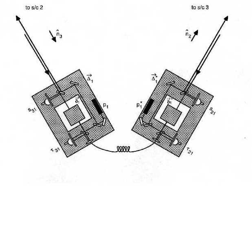
Figure 2: Schematic diagram of proof-masses-plus-optical-benches for a LISA spacecraft. The left-hand bench, $1$, reads out the phase signals $s_{31}$ and $\tau_{31}$. The right hand bench, $1^{*}$, analogously reads out $s_{21}$ and $\tau_{21}$. The random displacements of the two proof masses and two optical benches are indicated (lower case $\vec{\delta}_{i}$ for the proof masses, upper case $\vec{\Delta}_{i}$ for the optical benches.)

Beams between adjacent optical benches within a single spacecraft are bounced off proof masses in the opposite way. Light to be transmitted from the laser on an optical bench is first bounced off the proof mass it encloses and then directed to the other optical bench. Upon reception it does not interact with the proof mass there, but is directly mixed with local laser light, and again down converted. These data are denoted $\tau_{31}$ and $\tau_{21}$ in figure 2.

The terms in the following equations for the $s_{ij}$ and $\tau_{ij}$ phase measurements can now be developed from figures 1 and 2, and they are for the particular LISA configuration in which all the lasers have the same nominal frequency $\nu_{0}$, and the spacecraft are stationary with respect to each other. The analysis covering the configuration with lasers of different frequencies and spacecraft moving relative to each other was done in 2 , and we refer the reader to that paper.

Consider the $s_{31}(t)$ process (equation (3)) below. The photo receiver on the left bench of spacecraft $1$, which (in the spacecraft frame) experiences a time-varying displacement $\vec{\Delta}_{1}$, measures the phase difference $s_{31}$ by first mixing the beam from the distant optical bench $2^{*}$ in direction $\hat{n}_{3}$, and laser phase noise $p^{*}_{2}$ and optical bench motion $\vec{\Delta}^{*}_{2}$ that have been delayed by propagation along $L_{3}$, after one bounce off the proof mass ($\vec{\delta}_{1}$), with the local laser light (with phase noise $p_{1}$). Since for this simplified configuration no frequency offsets are present, there is of course no need for any heterodyne conversion.

In equation (4) the $\tau_{31}$ measurement results from light originating at the right-bench laser ($p^{*}_{1}$, $\vec{\Delta}^{*}_{1}$), bounced once off the right proof mass ($\vec{\delta}^{*}_{1}$), and directed through the fiber (incurring phase shift $\mu_{1}(t)$), to the left bench, where it is mixed with laser light ($p_{1}$). Similarly the right bench records the phase differences $s_{21}$ and $\tau_{21}$. The laser noises, the gravitational wave signals, the optical path noises, and proof-mass and bench noises, enter into the four data streams recorded at vertex $1$ according to the following expressions 2

$$s_{21} = s^{\rm gw}_{21}+s^{\rm opt.\ path}_{21}+p_{3,2}-p^{*}_{1}+\nu_{0}\ \left[2{\hat{n}_{2}}\cdot{\vec{\delta}^{*}_{1}}-{\hat{n}_{2}}\cdot{\vec{\Delta}^{*}_{1}}-{\hat{n}_{2}}\cdot{\vec{\Delta}_{3,2}}\right]\ ,$$ (1)

$$\tau_{21} = p_{1}-p^{*}_{1}+2\ \nu_{0}\ {\hat{n}_{3}}\cdot({\vec{\delta}_{1}}-{\vec{\Delta}_{1}})+\mu_{1}\ ,$$ (2)

$$s_{31} = s^{\rm gw}_{31}+s^{\rm opt.\ path}_{31}+p^{*}_{2,3}-p_{1}+\nu_{0}\ \left[-\ 2{\hat{n}_{3}}\cdot{\vec{\delta}_{1}}+{\hat{n}_{3}}\cdot{\vec{\Delta}_{1}}+{\hat{n}_{3}}\cdot{\vec{\Delta}^{*}_{2,3}}\right]\ ,$$ (3)

$$\tau_{31} = p^{*}_{1}-p_{1}-\ 2\ \nu_{0}\ {\hat{n}_{2}}\cdot({\vec{\delta}^{*}_{1}}-{\vec{\Delta}^{*}_{1}})+\mu_{1}\ .$$ (4)

Eight other relations, for the readouts at vertices 2 and 3, are given by cyclic permutation of the indices in equations (1)-(4).

The gravitational wave phase signal components, $s^{\rm gw}_{ij}\ ,\ i,j=1,2,3$, in equations (1) and (3) are given by integrating with respect to time the equations (1), (2) of reference 5 that relate metric perturbations to frequency shifts. The optical path phase noise contributions, $s^{\rm opt.\ path}_{ij}$, which includes shot noise from the low signal-to-noise ratio (SNR) in the links between the distant spacecraft, can be derived from the corresponding term given in 3 . The $\tau_{ij}$ measurements will be made with high SNR so that for them the shot noise is negligible.

The laser-noise-free combinations of phase data can readily be obtained from those given in 3 for frequency data. We use the same notations: $X$, $Y$, $Z$, $\alpha$, $\beta$, $\gamma$, $\zeta$, etc., but the reader should keep in mind that here these are phase measurements.

The phase fluctuations, $s_{ij}\ ,\ \tau_{ij}\ ,\ i,j=1,2,3$, are the fundamental measurements needed to synthesize all the interferometric observables unaffected by laser and optical bench noises. If we assume for the moment these phase measurements to be continuous functions of time, the three armlengths to be perfectly known and constant, and the three clocks onboard the spacecraft to be perfectly synchronized, then it is possible to cancel out exactly the phase fluctuations due to the six lasers and six optical benches by properly time-shifting and linearly combining the twelve measurements $s_{ij}\ ,\ \tau_{ij}\ ,\ i,j=1,2,3$. The simplest such combination, the totally symmetrized Sagnac response $\zeta$, uses all the data of Figure 2 symmetrically

$$\zeta = s_{32,2}-s_{23,3}+s_{13,3}-s_{31,1}+s_{21,1}-s_{12,2}$$ (5)

$$+{1\over 2}[({\tau_{23}}-{\tau_{13}})_{,12}+({\tau_{31}}-{\tau_{21}})_{,23}+({\tau_{12}}-{\tau_{32}})_{,13}]$$

$$+{1\over 2}[({\tau_{23}}-{\tau_{13}})_{,3}+({\tau_{31}}-{\tau_{21}})_{,1}+({\tau_{12}}-{\tau_{32}})_{,2}],$$

and its transfer functions to instrumental noises and gravitational waves are given in 3 and 5 respectively. In particular, $\zeta$ has a “six-pulse response” to gravitational radiation, i.e. a $\delta$-function gravitational wave signal produces six distinct pulses in $\zeta$ 5 , which are located with relative times depending on the arrival direction of the wave and the detector configuration.

Together with $\zeta$, three more interferometric combinations, ($\alpha,\beta,\gamma$), jointly generate the entire space of interferometric combinations 3 , 5 , 6 . Their expressions in terms of the measurements $s_{ij}$, $\tau_{ij}$ are as follows

$$\alpha = s_{21}-s_{31}+s_{13,2}-s_{12,3}+s_{32,12}-s_{23,13}+{1\over 2}\ [({\tau_{23}}-{\tau_{13}})_{,2}+({\tau_{23}}-{\tau_{13}})_{,13}+({\tau_{31}}-{\tau_{21}})$$ (6)

$$\ +\ ({\tau_{31}}-{\tau_{21}})_{,123}+({\tau_{12}}-{\tau_{32}})_{,3}+({\tau_{12}}-{\tau_{32}})_{,12}]\ ,$$

with $\beta$, and $\gamma$ derived by permuting the spacecraft indices in $\alpha$. Like in the case of $\zeta$, a $\delta$-function gravitational wave produces six pulses in $\alpha$, $\beta$, and $\gamma$. In equations (5, 6) it is important to notice that the $\tau_{ij}$ measurements from each spacecraft always enter into the interferometric measurements as differences taken at the same time. This property naturally suggests a locking configuration that makes these differences equal to zero, as we will show in the next section.

We remind the reader that the four interferometric responses ($\alpha,\beta,\gamma,\zeta$) satisfy the following relationship

$$\zeta-\zeta_{,123}=\alpha_{,1}-\alpha_{,23}+\beta_{,2}-\beta_{,13}+\gamma_{,3}-\gamma_{,12}\ .$$ (7)

Jointly they also give the expressions of the interferometric combinations derived in 3 , 5 : the Unequal-arm Michelson (${\rm X},{\rm Y},{\rm Z}$), the Beacon (${\rm P},{\rm Q},{\rm R}$), the Monitor (${\rm E},{\rm F},{\rm G}$), and the Relay (${\rm U},{\rm V},{\rm W}$) responses

$${\rm X}_{,1} = \alpha_{,23}-\beta_{,2}-\gamma_{,3}+\zeta\ ,$$ (8)

$${\rm P} = \zeta-\alpha_{,1}\ ,$$ (9)

$${\rm E} = \alpha-\zeta_{,1}\ ,$$ (10)

$${\rm U} = \gamma_{,1}-\beta\ ,$$ (11)

with the remaining expressions obtained from equations (8, 9, 10, 11) by permutation of the spacecraft indices. All these interferometric combinations have been shown to add robustness to the mission with respect to failures of subsystems, and potential design, implementation, or cost advantages 3 , 5 .

II.1 Locking Conditions

The space of all possible interferometric combinations can be generated by properly time shifting and linearly combining the four combinations ($\alpha,\beta,\gamma,\zeta$), as given above. Although they have been derived by applying TDI to the twelve one-way Doppler data, in what follows we will show that they can also be written in terms of properly selected and time shifted two-way and one-way Doppler measurements. These can be generated by phase locking five of the six lasers to one of them, as it is described below.

Assume, without loss of generality, the laser on bench $1^{*}$ to be the master. Although there are several other possible locking schemes, the one chosen minimizes the number of locking conditions between the master and any given slave. Furthermore, locking schemes relying on more than one master could be implemented, but we will not address those in this paper. We will also assume the spacecraft to be stationary relative to each other. This assumption simplifies the analysis, and does not affect the validity of the general result 8 .

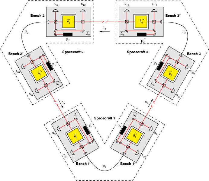
Figure 3: Simplified optical layout of the LISA interferometer, showing all the optical benches, proof masses and lasers.

Under this assumption, the frequency provided by the master laser $1^{*}$ can be used as input reference for the slaved lasers. In other words the slaves will then have the same center frequency as the master, and their phase fluctuations will be related to the fluctuations of the master laser as well as any other fluctuations introduced into the received light beam prior to reception and locking.

In order to understand the topology of the beams as the various slaves are locked to the master, let us follow the light paths from the master laser, $1^{*}$, to the slaves, as shown in Figure 3. Let us start first with the light beam that is bounced off the back of the proof-mass $1^{*}$. This beam is then directed to the other bench, $1$, where it is used as the input frequency reference for the laser there, and the measurement $\tau_{31}$ is made. Light is then re-transmitted back to bench $1^{*}$ where the measurement $\tau_{21}$ is performed. Since the phase of the laser $1$ is locked to that of the master, the relative phase fluctuations $\tau_{31}$ can be adjusted as follows

$$\tau_{31}=\tau_{21}\ ,$$ (12)

where we have assumed the noise introduced by phase-locking to be negligible (on this point see the theoretical derivations in Section III and Appendix A). Similarly, light beams from lasers $1$ and $1^{*}$ are transmitted to the lasers on the benches $2^{*}$ and $3$ respectively, where the lasers are locked to the incoming beams. From benches $2^{*}$ and $3$ beams are transmitted to the lasers on benches $2$ and $3^{*}$ respectively, where again locking is performed similarly to what is done onboard spacecraft $1$. Finally, along arm $1$, only two one-way relative phase measurements can be performed as it is easy to see. Since for the moment we have assumed a configuration with stationary spacecraft, the optical configuration described above can be translated into the following locking conditions on some relative phase fluctuation measurements

$$\tau_{31}=\tau_{21}\ \ \ \ ,\ \ \ \ \tau_{13}=\tau_{23}\ \ \ \ ,\ \ \ \ \tau_{32}=\tau_{12}\ \ \ \ ,\ \ \ \ s_{23}=s_{32}=0\ .$$ (13)

The locking conditions define specific relationships among the phase fluctuations from various noise sources. As an example, the conditions

$$\tau_{31}=\tau_{21}\ \ \ \ ,\ \ \ \ s_{23}=0\ ,$$ (14)

imply the following relationships among the laser phase fluctuations, the proof-mass noises, the gravitational wave signal, and the two bench noises onboard spacecraft $1$

$$p^{*}_{1} = p_{1}+\nu_{0}\ {\hat{n}_{3}}\cdot({\vec{\delta}_{1}}-{\vec{\Delta}_{1}})+\nu_{0}\ {\hat{n}_{2}}\cdot({\vec{\delta}^{*}_{1}}-{\vec{\Delta}^{*}_{1}})\ ,$$ (15)

$$0 = s^{\rm gw}_{23}+s^{\rm opt.\ path}_{23}+p^{*}_{1,2}-p_{3}+\nu_{0}\ \left[-\ 2{\hat{n}_{2}}\cdot{\vec{\delta}_{3}}+{\hat{n}_{2}}\cdot{\vec{\Delta}_{3}}+{\hat{n}_{2}}\cdot{\vec{\Delta}^{*}_{1,2}}\right]\ ,$$ (16)

with similar expressions following from the other locking conditions given in equation (13).

If we now substitute the locking conditions into the expressions for ($\alpha,\beta,\gamma,\zeta$), we obtain their expressions in terms of the remaining measurements

$$\zeta_{lo.} = s_{13,3}-s_{31,1}+s_{21,1}-s_{12,2}\ ,$$ (17)

$$\alpha_{lo.} = s_{21}-s_{31}+s_{13,2}-s_{12,3}\ ,$$ (18)

$$\beta_{lo.} = -s_{12}+s_{21,3}+s_{13,23}-s_{31,12}\ ,$$ (19)

$$\gamma_{lo.} = s_{13}-s_{31,2}+s_{21,13}-s_{12,23}\ ,$$ (20)

where the data ($s_{12}$, $s_{13}$) are one-way, and ($s_{21}$, $s_{31}$) are effectively two-way Doppler measurements due to locking.

The verification that the combinations ($\alpha_{lo.},\beta_{lo.},\gamma_{lo.},\zeta_{lo.}$) exactly cancel the laser phase fluctuations as well as the fluctuations due to the mechanical vibrations of the optical benches, can be performed by substituting the locked phase processes (such as 15, 16) into the expressions for ($s_{12},s_{13},s_{21},s_{31}$) (which are given by equations (1, 3) and their permutations), and by further replacing them into equations (17 - 20).

The main result of implementing locking is quantitatively shown by equations (17 - 20) in that the number of measurements needed for constructing the entire space of interferometric combinations LISA will be able to generate is smaller by a factor of three than the number of measurements needed when only one-way data are used.

Once ($\alpha_{lo.},\beta_{lo.},\gamma_{lo.},\zeta_{lo.}$) are constructed according to the expressions given in equations (17 - 20), all the other interferometric combinations can be derived by applying the identities given in equations (8 - 11). As an example, it is straightforward to show that equation (8) implies the following expression for the unequal-arm Michelson combination $X_{lo.}$

$$X_{lo.}=[s_{21}-s_{31}]-[s_{21,33}-s_{31,22}]\ ,$$ (21)

which coincides with the expression for $X$, derived for the first time in 7 , in terms of the two-way Doppler measurements from the two LISA arms.

As a final comment, we have analyzed also several locking configurations needed when the spacecraft are moving relative to each other. We have found that there exist techniques, when locking is implemented, which are similar to the one analyzed in 2 for removing the noise of the onboard Ultra Stable Oscillators from the phase measurements. The conclusions derived above for the case of stationary spacecraft are therefore general, and an analysis covering locking configurations with moving spacecraft is available in 8 .

III Phase Locking Performance

The locking conditions given in equation (13) reflect the assumption that the noise due to the optical transponders is negligible. In this section we analyze the noise added by the process of locking the phase of the local laser to the phase of the received light. This noise will be in addition to the optical path and USO noises, which we consider separately.

A block diagram of the phase locking control system is shown in figure 4(a). The system consists of a photoreceiver, phasemeter, controller, actuator and laser (see section IV for a description of these subsystems). Each of these subsystems can be characterized by its transfer function and, when it applies, by a noise contribution Abramovici . The main inputs to the system are the phase noise of the local laser, $p_{L}(s)$, and the phase fluctuations of the signal beam from the distant spacecraft, $p_{S}(s)$ (with $s=\sigma+i\omega$ being the Laplace variable). The closed loop output is the phase noise of the retransmitted laser beam, $p_{CL}(s)$.

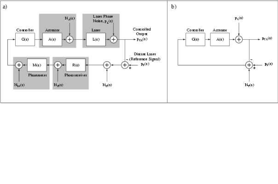
Figure 4: a) Block diagram of phase locking control system showing transfer functions and noise contributions of various system components. (b) Simplified control system block diagram.

From the block diagram shown in figure 4a, it is easy to see that the closed loop output phase $p_{CL}(s)$ can be written in terms of the free-running laser phase noise, $p_{L}(s)$, the input signal phase fluctuations, $p_{S}(s)$, and the various feedback components’ transfer functions and noises shown in Figure 4, as follows

$$p_{CL}=p_{L}+L\left\{N_{A}+A\ G\left[N_{M}+M\left(N_{R}+R\left\{N_{D}+p_{S}-p_{CL}\right\}\right)\right]\right\}\ .$$ (22)

This equation can be solved for $p_{CL}$

$$p_{CL}={{p_{L}+L\left\{N_{A}+A\ G\left[N_{M}+M\left(N_{R}+R\left\{N_{D}+p_{S}\right\}\right)\right]\right\}}\over{1+L\ A\ G\ M\ R}}\ ,$$ (23)

where we have denoted with $N_{R}(s)$, $N_{M}(s)$, and $N_{A}(s)$ the noises due to the photoreceiver, phasemeter, and actuator respectively. The detection noise, $N_{D}(s)$ is the error in the measurement of the relative phase of the two beams. This noise is the fundamental limit to the phase measurement process for the LISA detection system (see Appendix A). Since the link from the phasemeter to the controller will be digital, the controller noise will be due only to the finite precision of the digital phase information. We thus assume this noise to be negligible and do not include it in this analysis.

Since (i) the product $M(s)\ R(s)=1$ (the phase at the phasemeter output ought to be equal to the phase at the input point of the photoreceiver), (ii) the contribution of the actuator noise to the output, $L(s)N_{A}(s)$, is much smaller than the noise from the free-running laser (the free running laser noise is measured with the actuators attached and thus intrinsically contains this noise source), and (iii) the laser transfer function, $L(s)$, is a passive low pass filter with a pole at several GHz (and so can be ignored in this discussion), we conclude that the block diagram in 4 (a) now simplifies to that shown in figure 4(b), with the closed loop output now given by

$$p_{CL} = p_{L}+AG\left[N_{T}+p_{S}-p_{CL}\right]\ \ \ \longrightarrow p_{CL}=\frac{p_{L}+AG\left[N_{T}+p_{S}\right]}{1+AG}$$ (24)

$$p_{CL}-p_{S} \simeq N_{T}+\frac{p_{L}}{AG}\,\,\,\,\,(\rm{for}\,\,AG\gg 1)\ .$$ (25)

The quantity $N_{T}(s)$ is the total noise at the input to the controller and is given by

$$N_{T} = N_{M}+MN_{R}+N_{D})\ .$$ (26)

Equation (25) shows that phase locking will drive the phase of the local laser, $p_{CL}(s)$, to that of the received laser, $p_{S}(s)$, with an error introduced by two terms. The first term is the total measurement noise in the phase measurement, $N_{T}(s)$, which is in turn determined by the detection noise, photoreceiver noise and phasemeter noise (see equation 26). Recall that the detection noise, $N_{D}(s)$, is the fundamental error in the measurement of the relative phase of the two beams for the LISA detection system. A rigorous calculation of this noise source, included in appendix A, shows that its root power spectral density is equal to $\sim 1~{}\mu{\rm cycle}/\sqrt{\rm Hz}$ at the output of the phase meter. $N_{R}(s)$ is the electronic noise of the photoreceiver at the beat note frequency. Referenced to the output of the phasemeter this will be well below the $1~{}\mu{\rm cycle}/\sqrt{\rm Hz}$ level. A phasemeter noise floor of $\sim 1~{}\mu{\rm cycle}/\sqrt{\rm Hz}$ has been set as a requirement for the phasemeter noise. This level of performance has already been demonstrated (8bis , 8SHA ) over the frequency range of interest (1 mHz to 1 Hz) albeit with heterodyne frequencies of a few kilohertz . Given these estimates of the individual noise sources a total measurement error, $N_{T}(s)$ of less than $2\ \mu{\rm cycles}/\sqrt{\rm Hz}$ is expected.

The second source of error in Eq. (25) represents the finite suppression of the free running laser noise. This term is inversely proportional to the loop gain and so can be reduced by increasing the gain. Very high gains should be possible with LISA as the frequencies of interest are very low Abramovici , $\approx 10$  Hz and lower. A free-running laser frequency noise of 1 MHz/$\sqrt{\rm Hz}$ at 1 mHz corresponds to a phase noise of $10^{9}$ cycles/$\sqrt{\rm Hz}$. A total loop gain of $10^{15}$ is therefore required to suppress the contribution of laser frequency noise down to 1 $\mu{\rm cycle}/\sqrt{\rm Hz}$. At low frequencies the laser phase is altered by changing the temperature of the laser crystal. This actuator has a typical (voltage to frequency) gain of 5 GHz/Volt or $5\times 10^{12}~{}{\rm cycles}/\sqrt{\rm Hz}$ at 1 mHz. Thus a controller gain of 200 V/cycle is needed. This gain requirement could be eased by “pre-stabilizing” the laser frequency, for example by locking to a low finesse cavity or other frequency reference. Initial results from bench top experiments (McNamaraPL ,Ye ) indicate that loop gains of the order of $10^{15}$ should be achievable, and hence that pre-stabilization may not be necessary.

The master-slave configuration phase locking requirement should be that the noise introduced by the locking process is insignificant compared to the $20~{}\mu{\rm cycle}/\sqrt{\rm Hz}$ of optical path noise allocated in the LISA noise budget 1 . As the analysis above has shown, phase locking is limited only by the measurement noise (assuming adequate gain). This measurement noise is common to both the one-way and the master-slave schemes and so, given adequate gain of the phase locking loop, there will be no difference in the performance of the two systems.

IV Hardware Requirements

In this section we compare the hardware needed by the two implementations of TDI discussed in the previous sections. The discussion will focus on the minimum hardware requirements and will not fully consider redundancy or fallback options. We will consider LISA as composed of several basic subsystems, and compare the type and quantity of the components required by each scheme.

IV.1 Laser Frequency Stabilization System

Both schemes rely on a sufficiently high laser frequency stability. This is because the cancellation of laser frequency noise via TDI is not exact due to finite accuracy of the arm length knowledge, finite timing accuracy, imperfect clock synchronization, and sampling time jitters. The frequency stabilization system could be composed of either an optical cavity, a gas cell, or a combination of both. The output is an error signal proportional to the difference between the laser frequency and the resonance frequency of the reference. Assuming that an optical cavity is used as the frequency reference with a Pound-Drever-Hall locking PDH readout, the frequency stabilization system will consist of an electro-optic phase modulator, an optical cavity, a photoreceiver, a double-balanced mixer, and a low pass filter 8tris .

IV.2 Phasemeter

A phasemeter is a device capable of measuring the phase of a photoreceiver output relative to the local USO. One could distinguish between two types of phasemeter: single-quadrature phasemeters, denoted PM(S), and full-range phasemeters, denoted PM(F). An example of a single-quadrature phasemeter is a mixer. It will have only a limited linear range as the output is generally sinusoidal. A single-quadrature phasemeter has several potential advantages over a full-range phasemeter including lower noise, higher speed operation, increased reliability and lower power consumption. However, it is restricted in usefulness to closed loop operation only and is therefore not suitable for use in the one-way method. A single-quadrature phasemeter could potentially be used in the master-slaves configuration where one laser is phase locked to another with a fixed phase shift (see section IV. E).

A full-range phasemeter has an output that is linearly proportional to phase over the entire range $-\pi$ to $\pi$. An example of a full-range phasemeter is a zero-crossing time interval analyzer. As we show in section V. E, phasemeters used in an open-loop configuration must have a dynamic range of at least $\sim 10^{10}$ at $0.1$ mHz.

IV.3 Controller

A controller takes the signal from either a frequency stabilization system or phasemeter, amplifies and filters it appropriately, and feeds it back to the frequency/phase actuators of a laser. A controller is needed to frequency lock a laser to a frequency reference or to phase lock one laser to another. In practice the frequency locking and phase locking controllers will differ by a pole in the controller transfer function and by a gain factor. Depending on the sophistication of its design, a controller could potentially be reconfigured in-flight to perform either function.

IV.4 Photoreceivers

Each scheme requires twelve photoreceivers to measure the interference from the front and back of the proof masses. The photoreceiver unit will consist of a photodiode and low-noise electronic amplifiers. Although the photoreceivers for LISA will contain quadrant photodiodes for alignment sensing, this is irrelevant for the following discussion which assumes that single element photodiodes are used.

Spacecraft/Bench	Master-Slave Configuration	One-Way Method
SC $1^{*}$	1 FS, 2 PR, 2 PM(F), 1 Controller	1 FS, 2 PR, 2 PM(F), 1 Controller
SC 1	2 PR, 2 PM(F), 1 Controller	1 FS, 2 PR, 2 PM(F), 1 Controller
SC $2^{*}$	2 PR, 1 PM(F), 1 PM(S), 1 Controller	1 FS, 2 PR, 2 PM(F), 1 Controller
SC 2	2 PR, 2 PM(F), 1 Controller	1 FS, 2 PR, 2 PM(F), 1 Controller
SC $3^{*}$	2 PR, 2 PM(F), 1 Controller	1 FS, 2 PR, 2 PM(F), 1 Controller
SC 3	2 PR, 1 PM(F), 1 PM(S), 1 Controller	1 FS, 2 PR, 2 PM(F), 1 Controller

Table 1: Comparison of minimum system components required for each scheme. FS: frequency stabilization system, PM(S): single-quadrature phasemeter, PM(F) full-range phasemeter, PR: photoreceiver.

IV.5 Requirements for the Master-Slave Configuration

Table I summarizes the system components needed on each optical bench. The quantities shown represent the minimum requirements with no redundancy included. In the master-slave configuration scheme one master laser is frequency stabilized to its own frequency reference. All other lasers are phase locked in a chain to this master laser, as described in section IIA. For this reason the minimum system requirement is only one frequency stabilization system. However, the capability of stabilizing other lasers to a local stabilization system should be included for redundancy against failure of the master’s stabilizing device. Providing each laser with a frequency stabilization system would provide a high level of redundancy and maintain compatibility with the one-way mode of operation.

The master-slave configuration will require at least four full-range phasemeters for the main signal read out photoreceivers, $s_{21}$, $s_{31}$, $s_{12}$ and $s_{13}$. Full-range phasemeters will also be required for measuring the signals derived from the back side of the proof masses, $\tau_{ij}$, as the lasers on adjacent benches are locked by suppressing the difference of the phasemeter outputs, $\tau_{ij}-\tau_{kj}=0$. If just one of these phasemeter outputs were used for phase locking then a single-quadrature phasemeter could be utilized. However, the noise in the optical fiber linking the benches, $\mu_{i}$, would then be imposed on the phase of the slave laser. Although this noise would be removed by including the second detector in the time-delay interferometry processing, this would impose unnecessary requirements on the stability of the fiber link to prevent increasing the slave laser’s frequency noise. Furthermore, by suppressing the difference of these phasemeter outputs, we do not need to record this information for processing, as only the difference of the phasemeter outputs appears in the TDI equations (see for example, equations 5 and 6). Single-quadrature phasemeters could potentially be used on the remaining two photoreceivers where phase locking of the beams returning to spacecraft $1$ ($s_{23}=s_{32}=0$) is performed. This is a relatively minor simplification, as suitable full-range phasemeters must be developed for the remaining ten photoreceivers. If the phase locking hierarchy must be reordered, for example due to a frequency stabilization system failure, then full-range phasemeters will also be required at these positions. Finally, implementing full-range phasemeters at all photoreceiver outputs will maintain compatibility with the one-way method. For these reasons we will drop the (F) or (S) suffix for the phasemeters and assume that only full-range phasemeters are used.

Table II summarizes the total number of components required and the number of data streams to be recorded by each scheme. Using the master-slave configuration only four data streams remain to be measured ($s_{21}$, $s_{31}$, $s_{12}$ and $s_{13}$) as all other variables have been suppressed to effectively zero and therefore do not need to be recorded (although they should be monitored to ensure proper operation of the phase locking systems). One potential concern with the master-slave configuration is in the non-local nature of the control system, that is to say the main phase input to the control loop comes from the light from the distant spacecraft. The amplitude and phase of this beam could be adversely affected by many factors such as spacecraft alignment. Although this will also affect the quality of the one-way measurements, it could be more detrimental to the master-slave configuration. For example, the signal intensity could become so low to cause loss of phase lock entirely. Furthermore, because all the slaves are linked to the master by the phase-locking chain, if one phase-locking link is disrupted then all downstream links may also be lost. The severity of this non-local control problem depends on how often lock will be disrupted, and the difficulty of lock reacquisition.

Subsystem	Master-Slave Configuration	One-Way Method
FS	1	6
PR	12	12
PM	12	12
Controllers	6	6
Observables	4	9

Table 2: Summary of minimum system components required for each scheme. FS: frequency stabilization system, PM: phasemeter, PR: photoreceiver, Observables: number of data streams required for processing.

IV.6 Requirements for the One-way Method

The one-way method employs a very symmetric configuration consisting of three identical spacecraft each containing two identical optical benches. The components needed on each optical bench are shown in the right hand column of Table I. The six lasers are frequency stabilized to their six respective frequency references. The phases of the beat notes of each local laser with the lasers from the adjacent spacecraft and bench are measured by full-range phasemeters to provide twelve data streams. The data from the phasemeters at the back of the proof masses on adjacent benches can be combined before being recorded without loss of generality. This reduces the total number of data streams to be recorded and processed to nine, as shown in Table II. However, as we will show in section V C the number of data streams to be exchanged between spacecraft will be the same for the one-way and master-slaves configuration.

From Tables I and II it is clear that the one-way and master-slaves configurations are almost identical in terms of the quantity of components required. However, there are several more subtle differences in the hardware requirements of the two schemes. A disadvantage of the one-way method is that the laser frequencies may differ by as much as $\pm 300$ MHz if high finesse cavities are used as the frequency references. This maximum frequency offset is determined by the free spectral range of the reference cavity, where a cavity with a round trip optical path of 0.5 m has been assumed. This large frequency offset will place greater demands on the photoreceivers’ bandwidth than the master-slave configuration where frequency offsets can be kept to the minimum dictated by the Doppler shifts (less than $\pm 10$ MHz). Not only does the high heterodyne frequency place strict requirements on the photodetector bandwidth, but also on the bandwidth stability. For example, assume that photoreceivers with a bandwidth of $f_{bw}\approx 1$ GHz are used for the main signal readouts. Although a heterodyne frequency, $f_{h}$, of 300 MHz is within the 1 GHz photoreceiver bandwidth there will be a 0.05 cycle phase delay at this frequency (the phase shift is equal to -arctan$(f_{h}/f_{bw})$ radians for a simple single-pole type frequency response). If the bandwidth of a photodetector changes, then this phase shift will also change in a way that is indistinguishable from the effects of a gravitational wave. A simple calculation shows that a bandwidth change of a mere $0.023\%$ (or 230kHz) would introduce a phase signal of 10 $\mu$cycles/$\sqrt{\rm Hz}$ for information at 300 MHz. If the heterodyne frequency is kept to 10 MHz or less, then a photoreceiver bandwidth change of more than $0.6\%$ (or 6 MHz) would be needed to produce a 10 $\mu$cycles/$\sqrt{\rm Hz}$ phase shift.

In section III it was shown that a total loop gain of $10^{15}$ at 1 mHz is required to ensure that the phase locking loop performs correctly. Using the one-way method the phase locking loops are replaced by frequency locking to the reference cavity. The frequency stabilization system is expected to be limited by fluctuations in length of the cavity at a level of the order of 10 Hz/$\sqrt{\rm Hz}$ at 1 mHz. Under this condition no advantage is gained by suppressing the measured laser noise below this level and so a loop gain of $\approx 10^{6}$ should suffice. The one-way method therefore requires a controller gain of only $2\times 10^{-7}$ Volts/cycle at 1 mHz compared to the 200 Volts/cycle needed for the master-slave configuration.

V Accuracy and precision requirements

The limitations on the effectiveness of the TDI technique, either when the one-way or the master-slave configuration is implemented, come not only from all the secondary noise sources affecting the measurements $s_{ij}\ ,\ \tau_{ij}\ ,\ i,j=1,2,3$ (such as proof-mass and optical path noises) but most importantly from the finite accuracy and precision of the quantities needed to synthesize the laser-noise free observables themselves. In order to synthesize the four generators of the space of all interferometric combinations, we need:

(i) to know the distances between the three pairs of spacecraft;

(ii) to synchronize the clocks onboard the three spacecraft, which are used in the data acquisition and digitization process;

(iii) to be able to apply time-delays that are not integer multiples of the sampling time of the digitized phase measurements;

(iv) to minimize the effects of the jitter of the sampling times themselves; and

(v) to have sufficiently high dynamic range in the digitized data in order to be able to recover the gravitational wave signal after removing the laser noise.

In the following subsections we will assume the secondary random processes to be due to the proof masses and the optical path noises 3 . We will estimate the minimum values of the accuracies and precisions of the physical quantities listed above that allow the suppression of the laser frequency fluctuations below the level identified by the secondary noise sources. For each physical quantity the estimate of the accuracy and/or precision needed will be performed by assuming all the remaining errors to be equal to zero. Our estimates, therefore, will provide only an order of magnitude estimate of the accuracies and/or precisions needed for successfully implementing TDI.

V.1 Armlength accuracy

The TDI combinations described in the previous sections rely on the assumption of knowing the armlengths sufficiently accurately to suppress laser noise well below other noises. Since the three armlengths will be known only within the accuracies $\delta L_{i}\ ,\ i=1,2,3$ respectively, the cancellation of the laser frequency fluctuations from the combinations ($\alpha,\beta,\gamma,\zeta$) will no longer be exact. In order to estimate the magnitude of the laser fluctuations remaining in these data sets, let us define $\hat{L}_{i}\ ,\ i=1,2,3$ to be the estimated armlengths of LISA. They are related to the true armlengths $L_{i}\ ,\ i=1,2,3$, and the accuracies $\delta L_{i}\ ,\ i=1,2,3$ through the following expressions

$$\hat{L}_{i}=L_{i}+\delta L_{i}\ \ \ \ \ ,\ \ \ \ \ i=1,2,3\ .$$ (27)

In what follows we will treat the three armlengths $L_{i}\ ,\ i=1,2,3$ as constants equal to $16.7$ light seconds. We will derive later on the time scale during which such an assumption is valid. We will also assume to know with infinite accuracies and precisions all the remaining physical quantities needed to successfully synthesize the TDI generators.

If we now substitute equation (27) into equations (5), and expand it to first order in $\delta L_{i}$, it is easy to derive the following approximate expression for ${\hat{\zeta}}(t)$, which now will show a non-zero contribution from the laser noises

$${\hat{\zeta}}(t)\simeq\zeta(t)+[{\dot{p}}_{2,13}-{\dot{p}}^{*}_{3,12}]\ \delta L_{1}+[{\dot{p}}_{3,12}-{\dot{p}}^{*}_{1,23}]\ \delta L_{2}+[{\dot{p}}_{1,23}-{\dot{p}}^{*}_{2,13}]\ \delta L_{3}\ ,$$ (28)

where the “${\dot{\ }}$” denotes time derivative. Time-Delay Interferometry can be considered effective if the magnitude of the remaining fluctuations from the lasers are smaller than the fluctuations due to the other noise sources entering in $\zeta(t)$, namely proof mass and optical path noises. This requirement implies a limit in the accuracies of the measured armlengths.

Let us assume the six laser phase fluctuations to be uncorrelated to each other, their one-sided power spectral densities to be equal, the three armlengths to differ by a few percent, and the three armlength accuracies also to be equal. By requiring the magnitude of the remaining laser noises to be smaller than the secondary noise sources, it is straightforward to derive, from Eq. (28) and the expressions for the proof mass and optical path noises entering into $\zeta(t)$ given in 3 , the following constraint on the common armlength accuracy $|\delta L_{\zeta}|$

$$|\delta L_{\zeta}|\leq\ {1\over{2\pi f}}\ \sqrt{{4\ \sin^{2}(\pi fL)\ S^{proof\ mass}_{p}(f)+S^{optical\ path}_{p}(f)}\over{S_{p}(f)}}\ .$$ (29)

Here $S_{p}$, $S^{proof\ mass}_{p}$, $S^{optical\ path}_{p}$ are the one-sided power spectral densities of the phase fluctuations of a stabilized laser, a single proof mass, and a single-link optical path respectively 3 . If we take them to be equal to the following functions of the Fourier frequency $f$ 2 ; 3

$$S_{p}(f) = 2.3\times 10^{-1}\ f^{-8/3}+1.4\times 10^{-9}\ f^{-27/5}\ {\rm cycles}^{2}\ {\rm Hz}^{-1}\ ,$$ (30)

$$S^{proof\ mass}_{p}(f) = 5.8\times 10^{-21}\ f^{-4}\ {\rm cycles}^{2}\ {\rm Hz}^{-1}\ ,$$ (31)

$$S^{optical\ path}_{p}(f) = 4.1\times 10^{-10}\ {\rm cycles}^{2}\ {\rm Hz}^{-1}\ ,$$ (32)

(where $f$ is in Hz), we find that the right-hand-side of the inequality given by equation (29) reaches its minimum of about $16$ meters at the Fourier frequency $f_{min}=1.0\ \times 10^{-4}\ {\rm Hz}$, over the assumed ($10^{-4},1$) Hz LISA band. This implies that, if the armlength knowledge $|\delta L_{\zeta}|$ can be made smaller than $16$ meters, the magnitude of the residual laser noise affecting the $\zeta$ combination will be below that identified by the secondary noises. This reflects the fact that the armlength accuracy is a decreasing function of the frequency. For instance, at $10^{-3}$ Hz the armlength accuracy goes up by almost an order of magnitude to about $155$ meters.

A perturbative analysis similar to the one described above can be performed for the remaining generators ($\alpha,\beta,\gamma$). We find that the corresponding inequality for the armlength accuracy required for the $\alpha$ combination, $|\delta L_{\alpha}|$, is equal to 3 ; 7

$$|\delta L_{\alpha}|\leq\ {1\over{2\pi f}}\ {\sqrt{{[8\ \sin^{2}(3\pi fL)+16\ \sin^{2}(\pi fL)]\ S^{proof\ mass}_{\phi}(f)+6\ S^{optical\ path}_{\phi}(f)}\over{6\ S_{p}(f)}}}\ ,$$ (33)

with similar inequalities also holding for $\beta$ and $\gamma$. Equation (33) implies a minimum of the function on the right-hand-side equal to about $31$ meters at the Fourier frequency $f_{min}=1.0\ \times 10^{-4}\ {\rm Hz}$, while at $10^{-3}$ Hz the armlength accuracy goes up to $180$ meters.

Armlength accuracies significantly smaller than the level derived above can be achieved by implementing laser ranging measurements along the three LISA arms 1 , and we do not expect this to be a limitation for TDI.

In relation to the accuracies derived above, it is interesting to calculate the time scales during which the armlengths will change by an amount equal to the accuracies themselves. This identifies the minimum time required before updating the armlength values in the TDI combinations.

It has been calculated by Folkner et al. 9 that the relative longitudinal speeds between the three pairs of spacecraft, during approximately the first year of the LISA mission, can be written in the following approximate form

$$V_{i,j}(t)=V^{(0)}_{i,j}\ \sin\left({{2\pi t}\over T_{i,j}}\right)\qquad\qquad(i,j)=(1,2)\ ;\ (1,3)\ ;\ (2,3)\ ,$$ (34)

where we have denoted with $(1,2),(1,3),(2,3)$ the three possible spacecraft pairs, $V^{(0)}_{i,j}$ is a constant velocity, and $T_{i,j}$ is the period for the pair $(i,j)$. In reference 9 it has also been shown that the LISA trajectory can be selected in such a way that two of the three arms’ rates of change are essentially equal during the first year of the mission. Following reference 9 , we will assume $V^{(0)}_{1,2}=V^{(0)}_{1,3}\neq V^{(0)}_{2,3}$, with $V^{(0)}_{1,2}=1$ m/s, $V^{(0)}_{2,3}=13$ m/s, $T_{1,2}=T_{1,3}\approx 4$ months, and $T_{2,3}\approx 1$ year. From equation (34) it is easy to derive the variation of each armlength, for example $\Delta L_{3}(t)$, as a function of the time $t$ and the time scale $\delta t$ during which it takes place

$$\Delta L_{3}(t)=V^{(0)}_{1,2}\ \sin\left({{2\pi t}\over T_{1,2}}\right)\delta t\ .$$ (35)

Equation (35) implies that a variation in armlength $\Delta L_{3}\approx 10\ {\rm m}$ can take place during different time scales, depending on when during the mission this change takes place. For instance, if $t\ll T_{1,2}$ we find that the armlength $L_{3}$ changes by more than its accuracy ($\approx 10$ meters) after a time $\delta t=2.3\times 10^{3}$ seconds. If however $t\simeq T_{1,2}/4$, the armlength will change by the same amount after only $\delta t\simeq 10$ seconds instead.

V.2 Clock synchronization accuracy

The effectiveness of the TDI data combinations requires the clocks onboard the three spacecraft to be synchronized. Since the clocks will be synchronized with a finite accuracy, the laser noises will no longer cancel out exactly and the fraction of the laser frequency fluctuations that will remain into the TDI combinations will be proportional to the magnitude of the synchronization accuracy. In order to identify the minimum level of off-synchronization among the clocks that can be tolerated, we will proceed by treating one of the three clocks (say the clock onboard spacecraft $1$) as the master clock defining the time for LISA, and the other two to be synchronized to it. The relativistic (Sagnac) time-delay effect due to the fact that the LISA trajectory is a combination of two rotations, each with a period of one year, will have to be accounted for in the synchronization procedure. This is a procedure well known in the field of time-transfer, and we refer the reader to the appropriate literature for discussions on this point 10 . Here we will disregard this relativistic effect, and assume it can be compensated for with an accuracy better than the actual synchronization accuracy we derive below.

Let us denote by $\delta t_{2}$, $\delta t_{3}$, the time accuracies (time-offsets) for the clocks onboard spacecraft $2$ and $3$ respectively. If $t$ is the time onboard spacecraft $1$, then what is believed to be time $t$ onboard spacecraft $2$ and $3$ is actually equal to the following times

$${\hat{t}_{2}}=t+\delta t_{2}\ ,$$ (36)

$${\hat{t}_{3}}=t+\delta t_{3}\ .$$ (37)

If we now substitute equations (36, 37) into the equation (5) for $\zeta$, for instance, and expand it to first order in $\delta t_{i}\ ,\ i=2,3$, it is easy to derive the following approximate expression for ${\hat{\zeta}}(t)$, which shows the following non-zero contribution from the laser noises

$${\hat{\zeta}}(t)\simeq\zeta(t)+[{\dot{p}}_{1,23}-{\dot{p}}^{*}_{3,12}+{\dot{p}}^{*}_{2,13}-{\dot{p}}_{2,13}]\ \delta t_{2}+[{\dot{p}}_{2,13}-{\dot{p}}^{*}_{1,23}+{\dot{p}}^{*}_{3,12}-{\dot{p}}_{3,12}]\ \delta t_{3}\ .$$ (38)

By requiring again the magnitude of the remaining fluctuations from the lasers to be smaller than the fluctuations due to the other (secondary) noise sources affecting $\zeta(t)$, it is possible to derive an upper limit for the accuracies of the synchronization of the clocks. If we assume again the six laser phase fluctuations to be uncorrelated to each other, their one-sided power spectral densities to be equal, the three armlengths to differ by a few percent, and the two time-offsets’ magnitudes to be equal, by requiring the magnitude of the remaining laser noises to be smaller than the secondary noise sources it is easy to derive the following constraint on the time synchronization accuracy $|\delta t_{\zeta}|$

$$|\delta t_{\zeta}|\leq\ {1\over{2\pi f}}\ \sqrt{{12\ \sin^{2}(\pi fL)\ S^{proof\ mass}_{p}(f)+3\ S^{optical\ path}_{p}(f)}\over{4\ S_{p}(f)}}\ ,$$ (39)

with $S_{p}$, $S^{proof\ mass}_{p}$, $S^{optical\ path}_{p}$ again as given in equations (30-32).

We find that the right-hand-side of the inequality given by equation (39) reaches its minimum of about $47$ nanoseconds at the Fourier frequency $f_{min}=1.0\ \times 10^{-4}\ {\rm Hz}$. In other words, clocks synchronized at a level of accuracy better than $47$ nanoseconds will imply a residual laser noise that is smaller than the secondary noise sources entering into the $\zeta$ combination.

An analysis similar to the one described above can be performed for the remaining generators ($\alpha,\beta,\gamma$). For them we find that the corresponding inequality for the accuracy in the synchronization of the clocks is now equal to

$$|\delta t_{\alpha}|\leq\ {1\over{2\pi f}}\ \sqrt{{[4\ \sin^{2}(3\pi fL)+8\ \sin^{2}(\pi fL)]\ S^{proof\ mass}_{p}(f)+3\ S^{optical\ path}_{p}(f)}\over{4\ S_{p}(f)}}\ ,$$ (40)

with equal expressions holding also for $\beta$ and $\gamma$. The function on the right-hand-side of equation (40) has a minimum equal to $88$ nanoseconds at the Fourier frequency $f_{min}=1.0\ \times 10^{-4}\ {\rm Hz}$. As for the armlength accuracies, also the timing accuracy requirements become less stringent at higher frequencies. At $10^{-3}$ Hz, for instance, the timing accuracy for $\zeta$ and $\alpha,\beta,\gamma$ go up to $446$ and $500$ ns respectively.

A $50$ ns accuracy translates into a $15$ meter armlength accuracy, which we argued earlier to be easily achievable by the use of laser ranging. We therefore expect the synchronization of the three clocks to be achievable at the level derived above.

V.3 Telemetered signals and their sampling

To reduce the LISA-to-Earth telemetry requirements, it is expected that the normal operational mode will not telemeter the phase time series to the ground directly. Rather, we expect the TDI observables to be computed at the LISA array, and then only the (relatively low data rate) laser-noise-free combinations transmitted to Earth. Thus, both implementations of TDI discussed in this paper (the one-way method and the master-slave configuration) require phase measurements data to be exchanged among the spacecraft in order to synthesize the four generators of the space of all interferometric combinations. Although it is clear that the master-slave configuration implies a smaller number of measurements than that required by the one-way method, the actual number of data that will need to be exchanged among the spacecraft can be made to be exactly the same for both, making their inter-spacecraft telemetry requirements identical. This can easily be understood by rewriting the four generators ($\alpha,\beta,\gamma,\zeta$) in the following forms

$$\zeta = [s_{21,1}-s_{31,1}]+{1\over 2}[({\tau_{31}}-{\tau_{21}})_{,1}+({\tau_{31}}-{\tau_{21}})_{,23}]$$ (41)

$$+[s_{32,2}-s_{12,2}]+{1\over 2}[({\tau_{12}}-{\tau_{32}})_{,2}+({\tau_{12}}-{\tau_{32}})_{,13}]$$

$$+[s_{13,3}-s_{23,3}]+{1\over 2}[({\tau_{23}}-{\tau_{13}})_{,3}+({\tau_{23}}-{\tau_{13}})_{,12}]\ ,$$

$$\alpha = [s_{21}-s_{31}]+{1\over 2}\ [({\tau_{31}}-{\tau_{21}})+({\tau_{31}}-{\tau_{21}})_{,123}]$$ (42)

$$+[s_{32,12}-s_{12,3}]+{1\over 2}\ [({\tau_{12}}-{\tau_{32}})_{,3}+({\tau_{12}}-{\tau_{32}})_{,12}]$$

$$+[s_{13,2}-s_{23,13}]+{1\over 2}\ [({\tau_{23}}-{\tau_{13}})_{,2}+({\tau_{23}}-{\tau_{13}})_{,13}]\ .$$

Equations (41, 42) show that each generator can be formed by summing three different linear combinations of the data, each involving phase measurements performed onboard only a specific spacecraft. As an example, let us assume without loss of generality that $\zeta$ will be synthesized onboard spacecraft $1$. This means that spacecraft $2$ and $3$ will simply need to telemeter to spacecraft $1$ the particular combinations of the measurements they have made, which enter into the $\zeta$ combination. Since the space of all the interferometric combinations can be constructed by using four generators ($\alpha,\beta,\gamma,\zeta$) we conclude that spacecraft $2$ and $3$ will each have to telemeter to spacecraft $1$ four uniquely defined combinations of the measurements they have performed.

The time-delay interferometric combinations require use of phase measurements that are time-shifted with enough accuracy to bring the laser phase noise below the secondary noise sources. The required time resolution in the time-shifts should be equal to about $\sim 50$ ns for shifts tens of seconds in size. This is because the correct sample of the shifted data should be as accurate as the armlength accuracy itself. It can be shown that performing the time-shifting, on data sampled at $\sim 10$ Hz, by using digital interpolation filters, does not provide the required accuracy to effectively cancel the laser phase noises (see Appendix B for a detailed calculation).

An alternative approach 11 for achieving a timing accuracy of at least $50$ ns would be to sample each measurement at $\sim 20$ MHz or higher and store $\sim 2.0\times 10^{9}$ samples in a ring buffer for obtaining the data points of this measurement at the needed times. The phasemeter would then average these measurements over a fixed time period (perhaps a tenth of a second) centered around the sampled times at which the phase measurements are needed. The data is then exchanged among the spacecraft and the TDI combinations are formed.

This method can however be further refined by actually sampling every phase difference a few times, each time at $\sim 10$ Hz, but with a delay between the start time of every sampled version of the same phase difference. That is, we envision triggering the phasemeter such that the time series are sampled at the times required to form the TDI combinations. In this case the limitation of the finite sampling time in the determination of the delayed phase measurement is replaced by the timing precision of the phase measurements, which can be many orders of magnitude smaller than the smallest sampling time of the phasemeter, as we will show below.

As a concrete example, the ($\alpha_{lo.},\beta_{lo.},\gamma_{lo.},\zeta_{lo.}$) basis in the master-slave configuration requires measurements $\{s_{21},s_{21,1},s_{21,3},s_{21,13},s_{31},s_{31,1},s_{31,2},s_{31,12}\}$ from spacecraft 1, measurements $\{s_{12},s_{12,2},s_{12,3},s_{12,23}\}$ from spacecraft 2, and measurements $\{s_{13},s_{13,2},s_{13,3},s_{13,23}\}$ from spacecraft 3. By sampling the data $s_{21}$ at the times $n/f_{s},n/f_{s}-L_{1},n/f_{s}-L_{3},n/f_{s}-L_{1}-L_{3}$, where $f_{s}\sim 10$ Hz is the sampling frequency, and $n=0,1,2,...$ (and similarly for $s_{12},s_{13}$ and $s_{31}$) we can obtain the entire data at the required times, these being limited only by the timing precision of the phasemeters, the time synchronization accuracies of the clocks, and the armlength accuracies. This scheme requires sampling each signal four times at a sampling frequency ($10$ Hz) much smaller than what would be needed if sampling the data to the granularity required by the TDI combinations. Of course to correctly sample at $10$ Hz we must first ensure that the signal frequency bandwidth is less than $5$ Hz to avoid aliasing problems.

In practice, the times at which every sample from a given signal are taken could be adjusted every $1/f_{s}$, in order to protect the quality of the laser noise cancellation against drifting armlengths. This requires an adequate model of the spacecraft orbits, which could be updated as needed from spacecraft ranging data.

V.4 Sampling time jitter

The sampling times of all the measurements needed for synthesizing the TDI combinations will not be constant, due to the intrinsic timing jitters of the digitizing systems (USOs and phasemeters). Within the digitizing system, the USO is expected to be the dominant source of time jittering in the sampled data. Presently existing, space qualified, USO can achieve an Allan standard deviation of about $10^{-13}$ for integration times from $1$ to $10000$ seconds. This timing stability translates into a time jitter of about $10^{-13}$ seconds over a period of $1$ second. A perturbative analysis including the three sampling time jitters due to the three clocks shows that any laser phase fluctuations remaining in the four TDI generators will also be proportional to the sampling time jitters. Since the latter are approximately four orders of magnitude smaller than the armlength and clocks synchronization accuracies derived earlier, we conclude that the magnitude of laser noise residual into the TDI combinations due to the sampling time jitters can be made negligible.

V.5 Data digitization and bit-accuracy requirement

As shown in figure 5, the maximum of the ratio of the laser noise and of the secondary noises phase fluctuation amplitudes occurs at the lower end of the LISA bandwidth, and is $\sim 10^{10}$ at 0.1 mHz. This corresponds to the minimum dynamic range for the phasemeters to correctly measure the laser fluctuations and the weaker signals simultaneously. An additional safety factor of $\sim 10$ should be sufficient to avoid saturation if the noises are well described by Gaussian statistics.

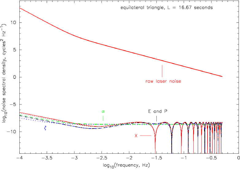
Figure 5: Phase fluctuations spectra are plotted versus Fourier frequency for: (upper curve) raw laser noise having spectral density $2.3\times 10^{-1}\ f^{-8/3}+1.4\times 10^{-9}\ f^{-27/5}\ {\rm cycles}^{2}\ {\rm Hz}^{-1}$, and (lower curves) residual noises entering into the various TDI combinations. The armlength has been assumed to be equal to $L=16.67\ {\rm sec}$.

In terms of requirements on the digital signal processing subsystem, this dynamic range implies that approximately $36$ bits are needed when combining the signals in TDI, only to bridge the gap between laser frequency noise and the other noises and gravitational wave signals. More bits might be necessary to provide enough information to efficiently filter the data when extracting weak gravitational wave signals embedded into noise.

VI Summary and Conclusions

A comparative analysis of different schemes for implementing Time-Delay Interferometry with LISA has been presented. In particular, we have shown that the master-slave configuration is capable of generating the entire space of interferometric combinations identical to that derived by using the one-way scheme. This was done under the assumption that the noise from the optical transponders was negligible. Our analysis of the phase-locking control systems forming the optical transponders shows that this is a valid assumption, indicating that the noise introduced can be expected to be $\approx 1\ \mu{\rm cycle}/\sqrt{\rm Hz}$.

A comparison of the hardware required for each scheme shows that the subsystems needed are almost identical, with the only difference being the number of frequency stabilization systems. This difference is perhaps not significant when redundancy options are considered. The main disadvantage of the one-way method is that the laser frequencies might be offset by several hundred megahertz, given the currently envisioned optical-cavity-based frequency stabilization systems. This places challenging constraints on the photoreceiver bandwidth and bandwidth stability. On the other hand, the master-slave configuration has no such problem, allowing the beat-note on the photoreceiver to be the minimum determined by the Doppler shift. However, there may be concerns with the non-local nature of the phase locking system, since its performance could be influenced, for example, by pointing stability (which also has implications on lock acquisition). Further studies on these issues should be performed.

Given the similarities between the two schemes, in principle either operational mode could be implemented without major implications on the hardware configuration. Ultimately detailed engineering studies will identify the preferred approach.

A derivation of the armlengths and clocks synchronization accuracies, as well as a determination of the precision requirement on the sampling time jitter, have also been derived. We found that an armlength accuracy of about 16 meters, a synchronization accuracy of about $50$ ns, and the time jitter due to a presently existing Ultra Stable Oscillator will allow the suppression of the frequency fluctuations of the lasers below the level identified by the secondary noise sources. A new procedure for sampling the data in such a way to avoid the problem of having time shifts that are not integer multiples of the sampling time was also presented, addressing one of the concerns about the implementation of Time-Delay Interferometry.

Appendix A Fundamental limit of the LISA phase transponder

The following is a derivation of the noise added by the optical phase measurement. This calculation only considers noise added by the detection system, it does not include the 20 $\mu$cycles$/\sqrt{\rm Hz}$ due to the optical-path noise, and it is purely quantum mechanical Bachor . The reason for performing the calculation in quantum mechanical terms is to highlight that the measurement process itself does not add shot noise and that, in principle, a perfect phase measurement of the field could be made.

Let us consider the optical configuration shown in figure 6(b), which is equivalent to the optical arrangement for the LISA interferometer (figure 6(a)). Let the annihilation operators for the local and distant lasers be $\hat{a}$ and $\hat{b}$ respectively. We can represent these operators as the sum of an average (complex number) component and an operator component representing the field fluctuations of zero mean values:

$$\hat{a} = \alpha+\delta\hat{a}\ ,$$ (43)

$$\hat{b} = \beta+\delta\hat{b}\ .$$ (44)

In Eqs. (43, 44) we define $\alpha$ and $\beta$ to be real numbers. We will assume throughout these calculations that $\delta\hat{a},\delta\hat{b}\ll\alpha,\beta$ and so terms that are of second order in these quantities will be ignored. This approximation holds even for the low intensities found in the LISA interferometer.

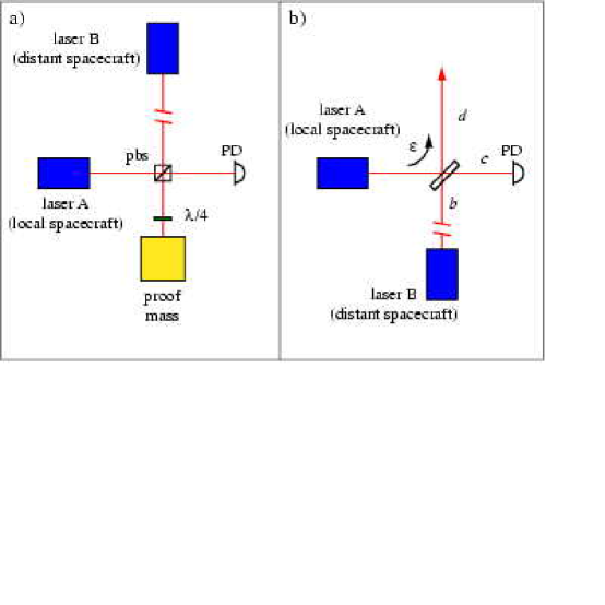
Figure 6: (a) Simplified optical arrangement for phase locking in LISA. (b) Equivalent optical layout for modeling purposes. $\epsilon$ is the intensity reflectivity of the beam splitter.

In an offset phase locking system the field $\hat{b}$ is offset from field $\hat{a}$ by a radial frequency $\omega_{b}$. In this case equations 43 and 44 become

$$\hat{a} = \alpha+\delta\hat{a}$$ (45)

$$\hat{b} = \beta{\rm e}^{i\omega_{b}t}+\delta\hat{b}{\rm e}^{i\omega_{b}t}\ .$$ (46)

The annihilation operator for the field at the photoreceiver, $\hat{c}$, will contain some fraction of $\hat{a}$ and $\hat{b}$,

$$\hat{c} = \sqrt{1-\epsilon}\,\hat{a}+\sqrt{\epsilon}\,\hat{b}\ .$$ (47)

The photoreceiver measures a quantity proportional to the photon number of this field, $n_{c}=\hat{c}^{\dagger}\hat{c}$,

$$\hat{c}^{\dagger}\hat{c} = (1-\epsilon)\left[\alpha^{2}+\alpha(\delta\hat{a}+\delta\hat{a}^{\dagger})\right]+\epsilon\left[\beta^{2}+\beta(\delta\hat{b}+\delta\hat{b}^{\dagger})\right]$$ (49)

$$+\sqrt{\epsilon}\sqrt{1-\epsilon}\left[\alpha\beta({\rm e}^{i\omega_{b}t}+{\rm e}^{-i\omega_{b}t})+\alpha(\delta\hat{b}{\rm e}^{i\omega_{b}t}+\delta\hat{b}^{\dagger}{\rm e}^{-i\omega_{b}t})+\beta(\delta\hat{a}{\rm e}^{-i\omega_{b}t}+\delta\hat{a}^{\dagger}{\rm e}^{i\omega_{b}t})\right]$$

$$= (1-\epsilon)\left[\alpha^{2}+\alpha(\delta\hat{a}+\delta\hat{a}^{\dagger})\right]+\epsilon\left[\beta^{2}+\beta(\delta\hat{b}+\delta\hat{b}^{\dagger})\right]$$

$$+2\sqrt{\epsilon}\sqrt{1-\epsilon}\Big{[}(\alpha\beta+\alpha(\delta\hat{b}+\delta\hat{b}^{\dagger})+\beta(\delta\hat{a}+\delta\hat{a}^{\dagger}))\cos(\omega_{b}t)$$

$$+(\alpha(i\delta\hat{b}-i\delta\hat{b}^{\dagger})-\beta(i\delta\hat{a}-i\delta\hat{a}^{\dagger}))\sin(\omega_{b}t)\Big{]}\ .$$

To simplify the notation, we define the quadrature operators which represent the fluctuations in the amplitude ($\delta\hat{X}^{+}$) and phase ($\delta\hat{X}^{-}$) quadratures of the operators $\hat{a}$ and $\hat{b}$,

$$\delta\hat{X}^{+}_{a} = (\delta\hat{a}+\delta\hat{a}^{\dagger})\ ,$$ (50)

$$\delta\hat{X}^{+}_{b} = (\delta\hat{b}+\delta\hat{b}^{\dagger})\ ,$$ (51)

$$\delta\hat{X}^{-}_{a} = i(\delta\hat{a}-\delta\hat{a}^{\dagger})\ ,$$ (52)

$$\delta\hat{X}^{-}_{b} = i(\delta\hat{b}-\delta\hat{b}^{\dagger})\ .$$ (53)

Each of these quantities is an observable of unit variance for a coherent state (idealized laser). Substituting these expressions into equation 49 we obtain,

$$\hat{c}^{\dagger}\hat{c} = (1-\epsilon)\left[\alpha^{2}+\alpha\delta\hat{X}^{+}_{a}\right]+\epsilon\left[\beta^{2}+\beta\delta\hat{X}^{+}_{b}\right]$$ (54)

$$+2\sqrt{\epsilon}\sqrt{1-\epsilon}\left[(\alpha\beta+\alpha\delta{X}^{+}_{b}+\beta\delta{X}^{+}_{a})\cos(\omega_{b}t)+(\alpha\delta{X}^{-}_{b}-\beta\delta{X}^{-}_{a})\sin(\omega_{b}t)\right]\ .$$

This equation contains three terms which can now be identified. The first two terms arise from the intensities of fields $\hat{a}$ and $\hat{b}$ respectively. These terms are non-interferometric in nature and contain the intensity fluctuations of the individual input beams scaled by the efficiency of coupling to the photoreceiver (beam splitter ratio). The third term represents the interference between the two fields and provides a beat note at frequency $\omega_{b}$, the difference frequency of the two fields. This beat note itself has two parts, an intensity noise part oscillating as $\cos(\omega_{b}t)$, and a phase difference part oscillating as $\sin(\omega_{b}t)$.

The phase difference can be obtained, for example, by using a mixer to demodulate the beat note down to zero. Mathematically, this is a multiplication by $\sin(\omega_{b}t)$. Terms with a cosine multiplier will only exhibit higher harmonics whereas terms with a sine multiplier will mixed down to base band frequencies.

After low-pass filtering the mixer output, we obtain the following expression for the error signal

$$V_{e} \equiv \frac{(1-\epsilon)}{2}\alpha\delta\hat{X}^{+}_{a,\omega_{b}}+\frac{\epsilon}{2}\beta\delta\hat{X}^{+}_{b,\omega_{b}}+\sqrt{\epsilon}\sqrt{1-\epsilon}(\alpha\delta{X}^{-}_{b}-\beta\delta{X}^{-}_{a})\ ,$$ (55)

where we have ignored the noise of the oscillator used in the mixing process. The quantities $\hat{X}^{+}_{a,\omega_{b}}$ and $\hat{X}^{+}_{b,\omega_{b}}$ are the amplitude quadrature operators evaluated at the offset frequency. The factor of 1/2 in the coefficients of these terms arises as we have only taken the sine component of the intensity noise at the heterodyne frequency. For heterodyne frequencies of 10 MHz and greater the intensity noise is shot noise limited thus $\langle(\hat{X}^{+}_{a,\omega_{b}})^{2}\rangle\approx\langle(\hat{X}^{+}_{b,\omega_{b}})^{2}\rangle\approx 1$. The important point is that the error signal is proportional to the intensity noise of each beam and the relative phase noise of the two lasers.

Assuming perfect phase locking, the error signal $V_{e}$ is driven to zero by actuating on the phase of $\hat{a}$. Setting $V_{e}=0$ we find that the controller will attempt to force the phase quadrature fluctuations to be,

$$\delta{X}^{-}_{a} = \frac{\alpha}{\beta}\delta{X}^{-}_{b}+\frac{\sqrt{1-\epsilon}\alpha\delta\hat{X}^{+}_{a,\omega_{b}}}{2\sqrt{\epsilon}\beta}+\frac{\sqrt{\epsilon}\delta\hat{X}^{+}_{b,\omega_{b}}}{2\sqrt{1-\epsilon}}\ .$$ (56)

Ultimately, what is of interest is the difference between the phases of the fields $\hat{d}$ and $\hat{a}$. The annihilation operator for the outgoing beam, $\hat{d}$, is also made up of a linear combination of $\hat{a}$ and $\hat{b}$

$$\hat{d} = \sqrt{\epsilon}\,\hat{a}-\sqrt{1-\epsilon}\,\hat{b}\ ,$$ (57)

which implies the following phase quadrature fluctuations of $\hat{d}$, $\delta\hat{X}^{-}_{d}$

$$\delta X^{-}_{d} = \sqrt{\epsilon}\delta\hat{X}^{-}_{a}-\sqrt{1-\epsilon}\delta\hat{X}^{-}_{b}\ .$$ (58)

Under the operational configuration of perfect phase locking, we can substitute into the equation above the expression for $\delta{X}^{-}_{a}$ given in equation 56

$$\delta X^{-}_{d} = (\sqrt{\epsilon}\frac{\alpha}{\beta}-\sqrt{1-\epsilon})\delta\hat{X}^{-}_{b}+\frac{\sqrt{1-\epsilon}\alpha\delta\hat{X}^{+}_{a,\omega_{b}}}{2\beta}+\frac{\epsilon\delta\hat{X}^{+}_{b,\omega_{b}}}{2\sqrt{1-\epsilon}}\ .$$ (59)

Since the power of the laser A (proportional to $\alpha^{2}$) will be a factor of $\approx 10^{8}$ larger than the power of laser B ( proportional to $\beta^{2}$), and also that $\langle(\delta\hat{X}^{+}_{b})^{2}\rangle\sim 1$, i.e. the signal laser intensity is approximately shot noise limited at the heterodyne frequency, we find that Eq. (59) can be approximated as follows

$$\delta X^{-}_{d} \simeq \frac{\alpha}{\beta}\left[\sqrt{\epsilon}\delta\hat{X}^{-}_{b}+\frac{\sqrt{1-\epsilon}\delta\hat{X}^{+}_{a,\omega_{b}}}{2}\right]\ .$$ (60)

The quantity of interest is the phase fluctuations in radians. To compare the phase fluctuations between the two fields we need to normalize the phase quadrature operator by the square root of the average photon number. For $\hat{d}$, this means dividing by $\sqrt{\epsilon}\alpha$

$$\delta\phi_{b} = \frac{\delta\hat{X}^{-}_{b}}{\beta}\ ,$$ (61)

$$\delta\phi_{d} = \frac{\delta\hat{X}^{-}_{b}}{\beta}+\frac{\sqrt{1-\epsilon}}{2\sqrt{\epsilon}}\frac{\delta\hat{X}^{+}_{a,\omega_{b}}}{\beta}\ .$$ (62)

Thus the phase of the incoming beam will differ from the phase of the outgoing beam by the following amount

$$\delta\phi_{d}-\delta\phi_{b} = \frac{\sqrt{1-\epsilon}}{2\sqrt{\epsilon}}\frac{\delta\hat{X}^{+}_{a,\omega_{b}}}{\beta}\ ,$$ (63)

while the root-mean-squared value of the phase error can be written as

$$\sigma_{\phi}=\sqrt{\frac{1-\epsilon}{4\epsilon}\frac{\langle|\delta\hat{X}^{+}_{a,\omega_{b}}|^{2}\rangle}{\bar{n}_{b}}}\ .$$ (64)

Here $\bar{n}_{b}=\beta^{2}$ is the average number of photons in the weak signal laser, and $\langle|\delta\hat{X}^{+}_{a,\omega_{b}}|^{2}\rangle$ is the variance of the local oscillator intensity fluctuations relative to the variance of quantum noise. Thus the error depends on two parameters, the beam splitter ratio and the intensity noise of the local oscillator. Assuming the local laser intensity is shot noise limited at the modulation frequency and a beam splitter ratio of approximately 100:1 ($\epsilon=0.99$) gives a phase error with a standard deviation, $\sigma_{\phi}$, of approximately $5\%$ of the shot noise limit or less than 1 $\mu$cycle$/\sqrt{\rm Hz}$ error. This error is therefore much less than the 20 $\mu$cycles$/\sqrt{\rm Hz}$ optical path noise.

If necessary, this source of error could be removed by altering the detection system to add a second detector allowing subtraction and consequent cancellation of the intensity noise of the local oscillator laser. Cancellation factors of 100 are readily achievable, albeit with a slight increase in system complexity, effectively removing this error contribution entirely.

Appendix B Interpolation error for generating shifted data points

Let $g(t)$ be the true signal. It is sampled at intervals $\Delta t=1/f_{s}$, where $f_{s}$ is the sampling frequency, to produce the discrete data $g[n]=g(t+n/f_{s})$, $n=...,-1,0,1,...$. Consider the problem of estimating $g(t)$ at some time which falls in between two sampling times, i.e. at time $t$ where $0<|t-n_{0}/f_{s}|<\Delta t$, for $n_{0}$ the value of $t/\Delta t$ rounded to the nearest integer. It is well known that for an infinitely long dataset, this estimation can be done without error using the Shannon formula 12 , assuming that the signal has zero power above the Nyquist frequency ($f_{s}/2$). The error in the estimation with a finite digital filter can be approximated using a truncated version of the Shannon formula. This digital filter might not be the best one for all signals, but it should be sufficiently close to the optimal filter. The estimated function is given by

$$g_{N}(t)=\sum_{n=-N}^{N}g[n+n_{0}]\;{\rm sinc}(f_{s}t-n-n_{0})\ ,$$ (65)

for a digital filter of length $2N+1$, and where $\;{\rm sinc}(x)=\sin(\pi x)/\pi x$. The estimation error is $e_{N}(t)=g(t)-g_{N}(t)$.

Changing the sampling frequency will not improve the function estimator for a fixed digital filter size: a lower sampling frequency would be insufficient to represent the high frequency signal components, and a higher sampling frequency would reduce the size of the interval over which the function is sampled to build the estimator.

Assuming $g(t)$ to be a wide sense stationary stochastic process 13 with autocorrelation function $R_{g}(|t_{1}-t_{2}|)=R_{g}(t_{1},t_{2})=E[g(t_{1})g(t_{2})]$ ($E[]$ denotes the expectation value), it follows that the autocorrelation function of the estimation error is equal to

$$R_{e_{N}}(t_{1},t_{2})=R_{g}(t_{1}-t_{2})+$$

$$\sum_{m,n=-N}^{N}R_{g}\left(\frac{n+n_{1}-m-n_{2}}{f_{s}}\right)\;{\rm sinc}(f_{s}t_{1}-n-n_{1})\;{\rm sinc}(f_{s}t_{2}-m-n_{2})$$

$$-\sum_{n=-N}^{N}R_{g}(t_{1}-n/f_{s}-n_{2}/f_{s})\;{\rm sinc}(f_{s}t_{2}-n-n_{2})$$

$$-\sum_{n=-N}^{N}R_{g}(t_{2}-n/f_{s}-n_{2}/f_{s})\;{\rm sinc}(f_{s}t_{1}-n-n_{1}),$$ (66)

where $n_{1}$ ($n_{2}$) is the value of $t_{1}/\Delta t$ ($t_{2}/\Delta t$) rounded to the nearest integer. This equation shows that $e_{N}(t)$ is not wide sense stationary; however, it is wide sense cyclo-stationary, since $R_{e_{N}}(t_{1},t_{2})=R_{e_{N}}(t_{1}+m\Delta t,t_{2}+m\Delta t)$ for every integer $m$. This is just a consequence of the error varying quasi-periodically with the interpolation time; it is zero when $t$ matches a sample time, maximum at the middle between two sample times, etc.

A fair estimate of the estimation error magnitude can be obtained by considering the stochastic process $\bar{e}_{N}(t)=e_{N}(t+\theta)$, where $\theta$ is a random variable uniformly distributed in $[0,\Delta t]$. $\bar{e}_{N}(t)$ is wide sense stationary, and its autocorrelation function is 13

$$R_{\bar{e}_{N}}(\tau)=f_{s}\int_{0}^{\Delta t}R_{e_{N}}(t+\tau,t)dt\ .$$ (67)

The Fourier transform of $R_{\bar{e}_{N}}(\tau)$ gives an estimate of the spectrum of the noise induced by the digital filters interpolation errors. In particular, $R_{\bar{e}_{N}}(0)$ is the broadband standard deviation of the noise.

Taking $g(t)$ to be a laser phase noise with a power spectral density that scales like $1/f^{2}$, and restricting attention to the frequency range 0.1 mHz $<f<$ 1 Hz, one can calculate numerically that $R_{\bar{e}_{N}}(0)/R_{g}(0)=9\times 10^{-7}$ for $N=10$. Therefore, a filter with $N=10$ is good enough only to produce a broadband error on the shifted time series that is $\sim 3$ orders of magnitude smaller than the laser phase noise amplitude. Changing $N$ in the numerical integrations shows that $R_{\bar{e}_{N}}(0)$ scales roughly like $1/N$. This implies that it would be impossible to use digital filters on a slowly sampled time series to achieve the levels of noise cancellation required by the TDI combinations.

References

- (1) P. Bender, K. Danzmann, & the LISA Study Team, Laser Interferometer Space Antenna for the Detection of Gravitational Waves, Pre-Phase A Report, (Max-Planck-Institüt für Quantenoptik, Garching), July 1998.
- (2) M. Tinto, F.B. Estabrook, & J.W. Armstrong, Phys. Rev. D, 65, 082003 (2002).
- (3) F.B. Estabrook, M. Tinto, & J.W. Armstrong, Phys. Rev. D, 62, 042002 (2000).
- (4) J. Gowar, Optical Communication Systems, (Prentice/Hall International, 1984), pp. 136-140.
- (5) J.W. Armstrong, F.B. Estabrook, & M. Tinto, Ap. J., 527, 814 (1999).
- (6) S.V. Dhurandhar, K.R. Nayak, & J.-Y. Vinet Phys. Rev. D, 65, 102002 (2002).
- (7) M. Tinto, & J.W. Armstrong Phys. Rev. D, 59, 102003 (1999).
- (8) D.A. Shaddock, Carrier-Sideband USO noise cancellation, available at the following URL address: , unpublished.
- (9) A. Abramovici and J. Chapsky, Feedback Control Systems a Fast-Track Guide for Scientists and Engineers, Kluwer Academic Publishers, Boston (2000).
- (10) O. Jennrich, R.T. Stebbins, P.L. Bender, and S. Pollack Clas. Quantum Grav., 18, 4159, (2001).
- (11) D.A. Shaddock, Digital I-Q Phasemeter by use of under-sampling. In Preparation.
- (12) P.W. McNamara, H. Ward, and J. Hough, Laser Phase Locking for LISA: Experimental Status. In: Proceedings of the Second International LISA Symposium on the Detection and Observation of Gravitational Waves in Space, ed. W.M. Folkner, AIP Conference Proceedings 456, Woodbury, New York, (1998).
- (13) J. Ye and J.L. Hall, Opt. Lett., 24, 1838, (1999)
- (14) R.W.P. Drever, J.L. Hall, F.V. Kowalski, J.Hough, G.M. Ford, A.J. Munley, and H.Ward, Appl. Phys. B, 31, 97 (1983).
- (15) P.W. McNamara, H. Ward, J. Hough, and D. Robertson, Clas. Quantum Grav., 14, 1543, (1997).
- (16) W.M. Folkner, F. Hechler, T.H. Sweetser, M.A. Vincent, and P.L. Bender, Clas. Quantum Grav., 14, 1405, (1997).
- (17) L. Schmidt, and M. Miranian, Common-View Time Transfer Using Multi-Channel GPS Receivers. In: Proceedings of the 29th Annual Precise Time and Time Interval (PTTI) Meeting, ed. L.A. Breakiron, United States Naval Observatory, (1997).
- (18) R.W. Hellings, Phys. Rev. D, 64, 022002 (2001)
- (19) H.A. Bachor and T.C. Ralph, A guide to experiments in Quantum Optics, John Wiley & Sons, New York (2003)
- (20) R.J. Marks, Introduction to Shannon sampling and interpolation theory, Springer-Verlag, Berlin (1991).
- (21) A. Papoulis, Probability, Random Variables, and Stochastic Processes, McGraw-Hill, New York, (1991).