On $3+1$ Dimensional Friedman-Robertson-Walker Universes with Matter

Abstract

We examine the dynamical behavior of matter coupled to gravity in the context of a linear Klein-Gordon equation coupled to a Friedman-Robertson-Walker metric. The resulting ordinary differential equations can be decoupled, the effect of gravity being traced in rendering the equation for the scalar field nonlinear. We obtain regular (in the massless case) and asymptotic (in the massive case) solutions for the resulting matter field and discuss their ensuing finite time blowup in the light of earlier findings. Finally, some potentially interesting connections of these blowups with features of focusing in the theory of nonlinear partial differential equations are outlined, suggesting the potential relevance of a nonlinear theory of quantum cosmology.

In the past two decades there has been an extensive interest in 3-dimensional gravity, particular after the demonstration of the fact that its quantum version is solvable [2] and that it contains black hole solutions [3].

The idea of examining cosmological models in this context was, however, of interest before [4, 5, 6], as well as after [7, 8] these findings. In most of these studies [4, 5, 6, 8], the Friedman-Robertson-Walker (FRW) metric was used and the resulting equations were ordinary differential equation governing the time-evolution of the scale factor of the relevant metric and the evolution of the matter and/or radiation field coupled to it.

On a slightly different track, one can list the works of [7, 9, 10] (see also references therein and the review of [11]), where the metric scale factors were allowed to be temporally as well as spatially variable, and the resulting partial-differential equations (PDEs) were studied to obtain collapse type solutions.

In this brief report, we will restrict ourselves to the former type of considerations (but in a 3+1 dimensional setting), namely fixing the spatial dependence of the metric tensor to be of the FRW type (in co-moving coordinates and with a “cosmological” time choice)

$$ds^{2}=-dt^{2}+a^{2}(t)\left(\frac{1}{1-kr^{2}}dr^{2}+r^{2}d\theta^{2}+r^{2}\sin^{2}\theta d\phi^{2}\right)$$ (1)

and coupling gravity to the simplest possible model for matter, namely a linear Klein-Gordon (KG) type equation for a massive scalar. In the metric of Eq. (1), $a$ is the scale factor while $k$ describes the curvature of the spatial slice and can be normalized to the values $-1,0,1$ in the hyperbolic, flat and elliptic case respectively. Previously such models were examined in a more complicated setting (most often in 2+1 dimensions) where either equations of state [8] or special scalar field potentials [5] were used to obtain closed form solutions.

Here, we will examine the simplest possible (physically relevant) scalar field potential $V(\phi)=m^{2}\phi^{2}/2$, which gives rise to a linear (in $\phi$) equation for the scalar coupled to gravity. In particular the Einstein-Klein-Gordon field equations in this case read:

$$-3\frac{k+\dot{a}^{2}}{a^{2}}+\rho_{\phi}=0$$ (2)

$$\frac{k+\dot{a}^{2}+2a\ddot{a}}{a^{2}}+p_{\phi}=0$$ (3)

$$\ddot{\phi}+m^{2}\phi+\frac{3\dot{a}}{a}\phi=0$$ (4)

where the energy density and the pressure associated with the scalar field are given respectively by (see e.g., [8])

$$\rho_{\phi}=\frac{1}{2}(\dot{\phi}^{2}+m^{2}\phi^{2})\equiv\frac{1}{2}\dot{\phi}^{2}+V(\phi),$$ (5)

$$p_{\phi}=\frac{1}{2}(\dot{\phi}^{2}-m^{2}\phi^{2})\equiv\frac{1}{2}\dot{\phi}^{2}-V(\phi).$$ (6)

Note that the first is the quadratic constraint $G^{0}_{0}=T^{0}_{0}$; the second is the only independent spatial equation $G^{1}_{1}=T^{1}_{1}$ while the last is the dynamical equation for the scalar field, i.e., the Klein-Gordon equation. $G$ and $T$ denote the Einstein curvature tensor and the energy-momentum tensor respectively.

In the above equations the dot denotes temporal derivative. Naturally, Eqs. (2)-(4) are not linearly independent as the linear combination of the derivative of the first and of the second can be used to obtain the third.

We first examine the spatially flat case of $k=0$, and use it as a guide. In this setting one immediately observes that from Eqs. (2) and (4), two separate expressions for $\dot{a}/a$ can be obtained, hence equating them, a second-order ordinary differential equation (ODE) emerges for the scalar field $\phi$ in the form:

$$\frac{3}{2}\dot{\phi}^{2}\left(m^{2}\phi^{2}+\dot{\phi}^{2}\right)=\left(m^{2}\phi+\ddot{\phi}\right)^{2}.$$ (7)

Notice that this is the only case (among the ones that we will examine) in which the resulting ODE is of 2nd order. In the remaining cases, the ODE is of 3rd order. Moreover, it is worth commenting on the nature of this ODE: in particular, the resulting equation is nonlinear. Hence, even though the inclusion of matter is realized through a linear dynamical equation, in the setting of even the simplest cosmological models, the coupling of matter to gravity induces the emergence of a nonlinear equation; it is as if the “trace” of gravity, when the equation for the scalar field is decoupled from it, remains in the nonlinearity of the resulting ODE.

As the simplest possible case among the ones with $k=0$, we examine the massless case, i.e., $m=0$. In the latter setting, we obtain the solutions (up to a constant shift) of the form:

$$\phi=\pm\sqrt{\frac{2}{3}}\log\left(t^{\star}-t\right)$$ (8)

which in turn results in a power law dependence of the scale factor of the form $a\sim(t^{\star}-t)^{1/3}$. Hence, a blowup (focusing) type effect occurs at $t=t^{\star}$ in a logarithmic fashion for the scalar and the corresponding scale factor shrinks to 0 with a power law dependence. Such dependencies are reminiscent of the critical blowup in prototypical nonlinear PDEs with focusing solutions (for a spatio-temporally dependent field $\psi$) such as the nonlinear Schrödinger equation [12, 13, 14]

$$i\psi_{t}=-\Delta\psi-|\psi|^{2\sigma}\psi.$$ (9)

$\Delta$ stands for the Laplacian and $\sigma$ the power of the nonlinearity. For $d\sigma<2$, no focusing solutions occur (d is the dimensionality of the Laplacian); when $d\sigma=2$, logarithmically slow focusing phenomena take place (in the corresponding “proper time” see [12, 13, 14]), while when $d\sigma>2$, the so-called strong collapse occurs, where the focusing happens with a power law dependence [13, 14]. Hence, the critical case of the nonlinear focusing phenomena in equation (9) shares some of the collapse characteristics of the present model.

We now turn to the massive case (still for $k=0$). In the latter, we can no longer solve the problem analytically. However, we can directly observe that if we adopt a solution of logarithmic dependence of the form of Eq. (8) in this case as well, the massive terms diverge much more slowly (at worst as $(\log(t^{\star}-t))^{2}/(t^{\star}-t)^{2}$, as opposed to the $(t^{\star}-t)^{-4}$ divergence of the dominant (massless) terms). This signifies that asymptotic self-similarity will ensue from this case and the logarithmic dependence will eventually set in and dominate the asymptotic behavior leading to collapse. An example of this is shown in Fig. 1, where a numerical simulation of Eq. (7) clearly indicates the logarithmic focusing of the scalar field for as $t\rightarrow 1.38$. This asymptotic type of self-similarity occurs quite often in cosmology, as can be seen for example in [15] (and references therein). One final comment worth making about this case is that it appears as if the massive case is asymptoting to the results for the massless one.

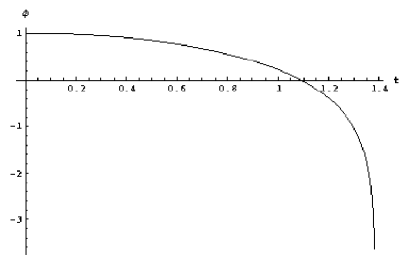
FIG. 1.: Logarithmic blowup of the scalar field as a function of time in the massive case (for $m=1$), starting with $\phi(0)=1$, $\dot{\phi}(0)=0$. The blowup occurs for $t\approx 1.38$.

We now turn to the case with $k\neq 0$. In this case also, the reduction that leads to an equation only for the scalar field can be performed. However, due to the more complex nature of the equations, this reduction no longer leads to a second order ODE but rather to a third order one. In particular, in this case the reduction (after differentiating (4) and substituting the result, as well as (2) and (4), in (3)) results in

$$6\dddot{\phi}\dot{\phi}-8\ddot{\phi}^{2}-10m^{2}\phi\ddot{\phi}-6\dot{\phi}^{4}+6m^{2}\dot{\phi}^{2}+3m^{2}\phi^{2}\dot{\phi}^{2}-2m^{4}\phi^{2}=0$$ (10)

It is interesting to note then that the massless case once again shares the exact same, finite time blowup solutions of Eq. (8). One can then once again use the same argument for the massive case to identify such solutions as the dominant asymptotic behavior for $m\neq 0$, since these terms blowup as $(t^{\star}-t)^{-4}$ in Eq. (10), while the rest of the terms diverge with a rate of (at most) $O(t^{\star}-t)^{-2}$. Numerical integration of Eq. (10) for various initial conditions and various masses confirms the theoretical prediction of finite time collapse. It appears however that the mass of the scalar affects the time at which collapse will occur ($t^{\star}$) (see e.g., Fig. 2).

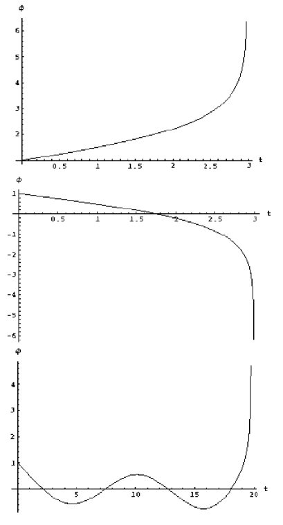
FIG. 2.: Logarithmic blowup of the scalar field as a function of time in the massive case (for $m=0.1$), starting with $\phi(0)=1$, $\dot{\phi}(0)=0.5$, $\ddot{\phi}(0)=0$ (top panel) and $\phi(0)=1$, $\dot{\phi}(0)=-0.5$, $\ddot{\phi}(0)=0$ (middle panel). The blowup occurs for $t\approx 3$ in these cases. A case with a larger mass ($m=0.6$) is shown in the bottom panel. In this case, the blowup occurs at later times (in this case for $t\approx 20$).

It is also worth noting that in the context of Eq. (10), the steady state $\phi=0$ appears to be linearly stable since for small perturbations $\sim\epsilon\exp(\omega t)$, collecting the leading order behavior (O($\epsilon^{2}$)), one obtains the algebraic stability equation of the form:

$$(\omega^{2}+m^{2})^{2}=0.$$ (11)

Eq. (11) has double imaginary roots:

$$\omega=\pm im$$ (12)

which, in turn, denote marginal stability. Notice that the same situation occurs in the critical case of Eq. (9). However, the nonlinear term of the form $-6\dot{\phi}^{4}$ asymptotically dominates and gives rise to a nonlinearity-induced instability leading to logarithmic blowup. This (blowup), in fact, is to be expected since the incompleteness of geodesics in $3+1$-dimensional spacetimes [16], established using general techniques of differential topology in [17, 18], has been shown under quite general conditions [19] to lead to divergence of physically observable properties.

In conclusion, in this work, we have examined the coupling of $3+1$-dimensional gravity to a scalar field satisfying a linear Klein-Gordon equation. We have found that it is possible to decouple the equation for the massive scalar from the one for the scale factor of the FRW metric used in this work at the “expense” of obtaining a nonlinear ordinary differential equation for the scalar. The “memory” of the coupling to gravity has been encapsulated in the nonlinear nature of the resulting equation. Closed form solutions of the resulting equation can be obtained in the massless case and exhibit logarithmic divergence of the scalar field as a function of time (and power-law vanishing of the scale factor). It is then observed that these solutions persist as dominant asymptotic behavior in the case where $m\neq 0$. These results are corroborated by numerical integration of the nonlinear ODEs in the massive case. Even though slightly different methods have been used for the cases where the metric is flat ($k=0$) and when $k\neq 0$, the same principal conclusions have been drawn in all cases.

This phenomenon of decoupling persists even in the case of more general, anisotropic Bianchi models [20]. In all these cases, special solutions to the ensuing decoupled non-linear ODE exist and they also exhibit blowup behavior.

Finally, we return to the analogy of the logarithmic focusing of the solutions in this simple model (where spatial dependence was a priori fixed in the metric) with the logarithmic blowup in the critical case of a prototypical nonlinear partial differential equation, namely the nonlinear Schrödinger equation, that sustains focusing solutions. It would be particularly interesting to examine whether the inclusion of spatial dependence can lead to an equation of this type (through appropriate envelope wave expansions, given that NLS is the envelope equation for nonlinear wave equations of the Klein-Gordon type). In particular, if, in the presence of the spatial dependence, the reduction to a nonlinear partial differential equation for the scalar field provides a nonlinear KG equation, then it will be natural to expect that the reduction to NLS and the ensuing focusing solutions will carry through. If such a program succeeds, it may appear natural to consider the NLS as prototypical model for a “nonlinear quantum cosmology”.

G.O. Papadopoulos is currently a scholar of the Greek State Scholarships Foundation (I.K.Y.) and acknowledges the relevant financial support. T Christodoulakis and G.O. Papadopoulos, acknowledge support by the University of Athens, Special Account for the Research Grant-No. 70/4/5000 This work was also partially supported by a University of Massachusetts Faculty Research Grant and NSF-DMS-0204585 (PGK), as well as the AFOSR (Dynamics and Control, IGK).

REFERENCES

- [1]
- [2] E. Witten, Nucl. Phys. B 311, 46 (1988).
- [3] M. Baados, C. Teitelboim and J. Zanelli, Phys. Rev. Lett. 69, 1849 (1992); M. Baados, M. Henneaux, C. Teitelboim and J. Zanelli, Phys. Rev. D 48, 1506 (1993).
- [4] S. Giddings, J. Abbott and K. Kuchar, Gen. Rel. Grav. 16, 751 (1984).
- [5] J.D. Barrow, A.B. Burd and D. Lancaster, Class. Quantum. Grav. 3, 551 (1986).
- [6] N.J. Cornish and N.E. Frankel, Phys. Rev. D 43, 2555 (1991).
- [7] M.W. Choptuik, gr-qc/9803075.
- [8] N. Cruz and C. Martínez, Class. Quantum Grav. 17, 2867 (2000).
- [9] T. Koike, T. Hara and S. Adachi, Phys. Rev. Lett. 74, 5170 (1995).
- [10] A.M. Abrahams and C.R. Evans, Phys. Rev. Lett. 70, 2980 (1993).
- [11] C. Gundlach, gr-qc/9712084.
- [12] M.J. Landman, G.C. Papanicolaou, C. Sulem and P.L. Sulem, Phys. Rev. A 38, 3837 (1988).
- [13] C. Sulem and P.-L. Sulem, The Nonlinear Schrödinger equation, Springer-Verlag (New York, 1999).
- [14] C.I. Siettos, I.G. Kevrekidis and P.G. Kevrekidis, Nonlinearity 16, 497 (2003).
- [15] B.J. Carr and A.A. Coley, Class. Quantum Grav. 16, R31 (1999).
- [16] S.W. Hawking and R. Penrose, Proc. R. Soc. A 314, 529 (1969).
- [17] S.W. Hawking and G.F.R. Ellis, The Large Scale Structure of Space-Time, Cambridge University Press (Cambridge, 1973).
- [18] F.J. Tipler, G.F.R. Ellis and C. Clarke, General Relativity and Gravitation, ed. A Held, pp 97-206, Plenum (New York, 1978).
- [19] C. Clarke, Commun. Math. Phys. 41, 65 (1975); C. Clarke and J. Isenberg, Proc. 9th Int. Conf. on General Relativity and Gravitation ed. E Schmutzer, Cambridge University Press (Cambridge, 1982).
- [20] T. Christodoulakis et al. (in preparation).