Causality and Superluminal Light

Abstract

The causal properties of curved spacetime, which underpin our sense of time in gravitational theories, are defined by the null cones of the spacetime metric. In classical general relativity, it is assumed that these coincide with the light cones determined by the physical propagation of light rays. However, the quantum vacuum acts as a dispersive medium for the propagation of light, since vacuum polarisation in QED induces interactions which effectively violate the strong equivalence principle (SEP). For low frequencies the phenomenon of gravitational birefringence occurs and indeed, for some metrics and polarisations, photons may acquire superluminal phase velocities. In this article, we review some of the remarkable features of SEP violating superluminal propagation in curved spacetime and discuss recent progress on the issue of dispersion, explaining why it is the high-frequency limit of the phase velocity that determines the characteristics of the effective wave equation and thus the physical causal structure.

1 Introduction

In general relativity, the nature of time and causality are determined by the properties of the null cones of the curved spacetime manifold. A physical realisation of these geometric null cones is provided in classical electrodynamics by the light cones traced by the propagation of light rays. As the title of this conference implies, ‘Time and Matter’ are therefore intimately related.

In quantum theory, however, the relationship is more subtle. Quantum effects such as vacuum polarisation in QED induce interactions which effectively violate the strong equivalence principle and cause the quantum vacuum in the presence of gravity to act as a dispersive medium for the propagation of light. At least for low frequencies, the phenomenon of gravitational birefringence occurs and moreover, for some metrics and polarisations, photons may acquire superluminal phase velocities. This forces a reassessment of the identification of light cones with null cones and raises the question of how causality and quantum theory can be reconciled in general relativity.

Research into this effect began with a key paper of Drummond and Hathrell[1] in which they calculated the one-loop vacuum polarisation contribution to the QED effective action in a background gravitational field. They found the following modification to the free Maxwell action:

$$\begin{array}[]{rcl}&\\ {}\hfil&\Gamma=\int dx\sqrt{-g}\biggl{[}-{1\over 4}F_{\mu\nu}F^{\mu\nu}\\[4.0pt] {}\hfil&+{1\over m^{2}}\biggl{(}aRF_{\mu\nu}F^{\mu\nu}+bR_{\mu\nu}F^{\mu\l}F^{\nu}{}_{\l}+cR_{\mu\nu\l\rho}F^{\mu\nu}F^{\l\rho}+dD_{\mu}F^{\mu\l}D_{\nu}F^{\nu}{}_{\l}\biggr{)}\biggr{]}\\ &&\end{array}$$ (1)

where $a$,$b$,$c$,$d$ are constants of $O(\alpha)$ and $m$ is the electron mass. The important feature is the direct coupling of the electromagnetic field to the curvature. This is an effective violation of the strong equivalence principle (SEP), which is the dynamical ansatz that the ‘laws of physics’ should be the same in the local inertial frames at each point in spacetime. (The weak equivalence principle, viz. the existence of such local inertial frames, is in contrast a fundamental assumption underlying the structure of general relativity.) More precisely, the SEP requires that electromagnetism is minimally coupled to gravity, i.e. through the connections only, independent of the curvature. The effective action Eq.(1) shows that while this principle may be consistently imposed at the classical level, it is necessarily violated in quantum electrodynamics. It is the quantum violation of the SEP that allows the physical light cones to differ from the geometric null cones.

The new SEP-violating interactions in Eq.(1) affect the propagation of light and modify the physical light cones. Using the techniques of geometric optics, Drummond and Hathrell showed that the new light cones are given by

$$k^{2}~{}-~{}{2b\over m^{2}}R_{\mu\l}k^{\mu}k^{\l}~{}+~{}{8c\over m^{2}}R_{\mu\nu\l\rho}k^{\mu}k^{\l}a^{\nu}a^{\rho}~{}~{}=~{}~{}0$$ (2)

where $k_{\mu}$ is the wave vector and $a_{\mu}$ the polarisation. Using the Einstein equations, this can be expressed as the sum of a ‘matter’ and a purely ‘gravitational’ contribution as follows:

$$k^{2}~{}-~{}{8\pi\over m^{2}}(2b+4c)T_{\mu\l}k^{\mu}k^{\l}~{}+~{}{8c\over m^{2}}C_{\mu\nu\l\rho}k^{\mu}k^{\l}a^{\nu}a^{\rho}~{}~{}=~{}~{}0$$ (3)

The first term involves the projection of the energy-momentum tensor which appears in the weak energy condition; this contribution is universal, appearing in the modified light cone condition for light propagating subluminally in a variety of backgrounds such as classical electromagnetic fields or finite temperature [2, 3, 4, 5]. The second term depends on the Weyl tensor and is uniquely gravitational; since it depends explicitly on the polarisation, the modified light cones exhibit gravitational birefringence.

It is also instructive to express Eqs.(2),(3) in the Newman-Penrose formalism. Introducing a null tetrad with basis vectors $\ell_{\mu}$, $n_{\mu}$, $m_{\mu}$ and $\bar{m}_{\mu}$ together with the corresponding components of the Ricci and Weyl tensors $\Phi_{00}=-{1\over 2}R_{\mu\nu}\ell^{\mu}\ell^{\nu}$, $\Psi_{0}~{}=~{}-C_{\mu\nu\l\rho}\ell^{\mu}m^{\nu}\ell^{\l}m^{\rho}$ etc. (for details, see ref.[4]), and choosing $\ell_{\mu}$ to coincide with the direction of propagation, i.e. $k_{\mu}=\omega\ell_{\mu}$, we find

$$k^{2}~{}-~{}{(4b+8c)\omega^{2}\over m^{2}}\Phi_{00}~{}~{}\pm~{}~{}{4c\omega^{2}\over m^{2}}(\Psi_{0}+\Psi_{0}^{*})~{}~{}=~{}~{}0$$ (4)

This representation makes it clear that the contribution from the Weyl tensor changes sign for the two physical transverse polarisations $a_{\mu}$. It follows immediately that for Ricci-flat spacetimes, both timelike and spacelike values of $k^{2}$ are possible. In other words, Eqs.(2),(3),(4) necessarily imply the existence of superluminal propagation. Physical photons no longer follow the geometrical null cones, but instead propagate on the effective, polarisation-dependent, light cones defined above.

Many examples of the Drummond-Hathrell effect in a variety of gravitational wave, black hole and cosmological spacetimes have been studied [1, 2, 6, 7]. The (Ricci-flat) black hole cases are particularly interesting, and it is found that for photons propagating orbitally, the light cones are modified such that superluminal propagation occurs. For radial geodesics in Schwarzschild spacetime, however, and the corresponding principal null geodesics in Reissner-Nordström and Kerr, the light cones are unchanged. The reason is simply that if we choose the standard Newman-Penrose tetrad in which $\ell^{\mu}$ is tangent to the principal null geodesic, the only non-vanishing component of the Weyl tensor is $\Psi_{2}$ since these black hole spacetimes are all Petrov type D, whereas the modification to the light cone condition involves only $\Psi_{0}$. Superluminal propagation is also predicted in the (Weyl-flat) FRW cosmological spacetimes, with the correction to the speed of light increasing as $1/t^{2}$ towards the initial singularity. Another interesting case involves the Bondi-Sachs metric describing gravitational radiation from an isolated source, where the magnitude of the superluminal effect is related to the peeling theorem for the Weyl tensor.

The existence of superluminal propagation in QED in curved spacetime of course raises immediate questions as to the realisation of causality. The purpose of this article is to review our research programme on photon propagation in gravitational fields with particular emphasis on the issue of causality and the consistency of quantum field theory with classical gravitation. We begin, in section 2, by considering carefully the implications of the Drummond-Hathrell effective action as it stands, reviewing the bimetric interpretation of the light cones, the realisation of stable causality in general relativity, possible time machine constructions and the consequences for event horizons.

However, the action Eq.(1) is only the lowest-order term in an expansion of the full effective action in powers of derivatives. That is, results derived from it are valid only in a low-frequency approximation $\l\gg\l_{c}$, where $\l_{c}$ is the electron Compton wavelength. The inclusion of terms of higher orders in derivatives shows that the propagation is in fact dispersive[8]. In section 3, we discuss the precise definition of the ‘speed of light’ and present a proof that the wavefront velocity, which is the relevant speed of light for causality, can be identified as the high-frequency limit of the phase velocity, $v_{\rm ph}(\infty)$. This means that a resolution of the issues raised in section 2 concerning causality depends on an explicit calculation of the light cones for high-frequency propagation. In section 4, we present a recently derived extension of the effective action valid to third order in curvatures and field strengths and to all orders in derivatives[9]. The resulting light cone is derived and some potential special features are described. Finally, however, we argue on the basis of a detailed comparison with photon propagation in background magnetic fields that a further, non-perturbative contribution to the effective action may ultimately control the high-frequency limit and we close with an assessment of the prospects for a final resolution of the question of dispersion and causality for QED in curved spacetime.

2 Causality and Superluminal Propagation

In this section, we discuss the implications for causality of photon propagation based on the Drummond-Hathrell action Eq.(1) and its associated light cones, setting aside for the moment the issue of dispersion.

2.1 Superluminal Propagation in Special and General Relativity

It is generally understood that superluminal propagation in special relativity leads to unacceptable violations of causality. Indeed the absence of tachyons is traditionally employed as a constraint on fundamental theories. We therefore begin by reviewing some basic features of superluminal propagation in order to sharpen these ideas in preparation for our subsequent discussion of causality in general relativity.

The first important observation is that given a superluminal signal we can always find a reference frame in which it is travelling backwards in time. This is illustrated in Fig. 1. Suppose we send a signal from O to A at speed $v>1$ (in $c=1$ units) in frame ${\cal S}$ with coordinates $(t,x)$. In a frame ${\cal S}^{\prime}$ moving with respect to ${\cal S}$ with velocity $u>{1\over v}$, the signal travels backwards in $t^{\prime}$ time, as follows immediately from the Lorentz transformation.

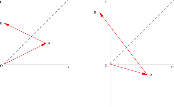
Figure 1: A superluminal $(v>1)$ signal OA which is forwards in time in frame ${\cal S}$ is backwards in time in a frame ${\cal S}^{\prime}$ moving relative to ${\cal S}$ with speed $u>{1\over v}$. However, the return path with the same speed in ${\cal S}$ arrives at B in the future light cone of O, independent of the frame.

The important point for our considerations is that this by itself does not necessarily imply a violation of causality. For this, we require that the signal can be returned from A to a point in the past light cone of O. However, if we return the signal from A to B with the same speed in frame ${\cal S}$, then of course it arrives at B in the future cone of O. The situation is physically equivalent in the Lorentz boosted frame ${\cal S}^{\prime}$ – the return signal travels forward in $t^{\prime}$ time and arrives at B in the future cone of O. This, unlike the assignment of spacetime coordinates, is a frame-independent statement.

The problem with causality arises from the scenario illustrated in Fig. 2.

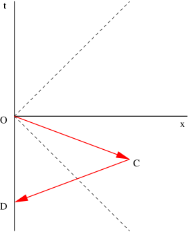
Figure 2: A superluminal $(v>1)$ signal OC which is backwards in time in frame ${\cal S}$ is returned at the same speed to point D in the past light cone of O, creating a closed time loop.

Clearly, if a backwards-in-time signal OC is possible in frame ${\cal S}$, then a return signal sent with the same speed will arrive at D in the past light cone of O creating a closed time loop OCDO. The crucial point is that local Lorentz invariance of the laws of motion implies that if a superluminal signal such as OA is possible, then so is one of type OC, since it is just given by an appropriate Lorentz boost (as in Fig. 1). The existence of global inertial frames then guarantees the existence of the return signal CD (in contrast to the situation in Fig. 1 viewed in the ${\cal S}^{\prime}$ frame).

The moral is that both conditions must be met in order to guarantee the occurrence of unacceptable closed time loops – the existence of a superluminal signal and global Lorentz invariance. Of course, since global Lorentz invariance (the existence of global inertial frames) is the essential part of the structure of special relativity, we recover the conventional wisdom that in this theory, superluminal propagation is indeed in conflict with causality.

The reason for presenting this elementary discussion is to emphasise that the situation is crucially different in general relativity. The weak equivalence principle, which we understand as the statement that a local inertial frame exists at each point in spacetime, implies that general relativity is formulated on a Riemannian manifold. However, local Lorentz invariance alone is not sufficient to establish the link between superluminal propagation and causality violation. This is usually established by adding a second, dynamical, assumption. The strong equivalence principle (SEP) states that the laws of physics should be identical in the local frames at different points in spacetime, and that they should reduce to their special relativistic forms at the origin of each local frame. It is the SEP which takes over the role of the existence of global inertial frames in special relativity in establishing the incompatibility of superluminal propagation and causality.

However, unlike the weak equivalence principle, which underpins the essential structure of general relativity, the SEP is merely a simplifying assumption about the dynamics of matter coupled to gravitational fields. Mathematically, it requires that matter or electromagnetism is minimally coupled to gravity, i.e. with interactions depending only on the connections but not the local curvature. This ensures that at the origin of a local frame, where the connections may be Lorentz transformed locally to zero, the dynamical equations recover their special relativistic form. In particular, the SEP is violated by interactions which explicitly involve the curvature, such as those occurring in the Drummond-Hathrell action (1) and the consequent modified light cones.

The question of whether this specific realisation of superluminal propagation is in conflict with causality is discussed in section 2.4 using the concept of stabele causality described in ref.[13]. Notice though that by violating the SEP, we have evaded the necessary association of superluminal motion with causality violation that held in special relativity. Referring back to the figures, what is established is the existence of a signal of type OA, which as we saw, does not by itself imply problems with causality even though frames such as ${\cal S}^{\prime}$ exist locally with respect to which motion is backwards in time. However, since the SEP is broken, even if a local frame exists in which the signal looks like OC, it does not follow that a return path CD is allowed. The signal propagation is fixed, determined locally by the spacetime curvature.

2.2 Geometric Optics

The most direct way to deduce the form of the light cones for QED in curved spacetime is to use geometric optics. This starts from the ansatz

$$(A_{\mu}+i\epsilon B_{\mu}+\ldots)\exp\bigl{(}i{\vartheta\over\epsilon}\bigr{)}$$ (5)

in which the electromagnetic field is written as a slowly-varying amplitude and a rapidly-varying phase. The parameter $\epsilon$ is introduced as a device to keep track of the relative order of magnitude of terms, and the Bianchi and Maxwell equations are solved order-by-order in $\epsilon$.

The wave vector is identified as the gradient of the phase, $k_{\mu}=\partial_{\mu}\vartheta$. We also write $A_{\mu}=Aa_{\mu}$, where $A$ represents the amplitude itself while $a_{\mu}$ specifies the polarisation, which satisfies $k_{\mu}a^{\mu}=0$.

Solving the usual Maxwell equation $D_{\mu}F^{\mu\nu}=0$, we find at $O(1/\epsilon)$,

$$k^{2}=0$$ (6)

while at $O(1)$,

$$k^{\mu}D_{\mu}a^{\nu}=0$$ (7)

and

$$k^{\mu}D_{\mu}(\ln A)=-{1\over 2}D_{\mu}k^{\mu}$$ (8)

Eq.(6) shows immediately that $k^{\mu}$ is a null vector. From its definition as a gradient, we also see

$$k^{\mu}D_{\mu}k^{\nu}=k^{\mu}D^{\nu}k_{\mu}={1\over 2}D^{\nu}k^{2}=0$$ (9)

Light rays, or equivalently photon trajectories, are the integral curves of $k^{\mu}$, i.e. the curves $x^{\mu}(s)$ where $dx^{\mu}/ds=k^{\mu}$. These curves therefore satisfy

$$0~{}=~{}k^{\mu}D_{\mu}k^{\nu}~{}=~{}{d^{2}x^{\nu}\over ds^{2}}+\Gamma^{\nu}_{\mu\l}{dx^{\mu}\over ds}{dx^{\l}\over ds}$$ (10)

This is the geodesic equation. We conclude that for the usual Maxwell theory in general relativity, light follows null geodesics. Eqs.(9),(7) show that both the wave vector and the polarisation are parallel transported along these null geodesic rays, while Eq.(8), whose r.h.s. is just (minus) the optical scalar $\theta$, shows how the amplitude changes as the beam of rays focuses or diverges.

2.3 Bimetricity

The same method is applied to the modified Maxwell equation derived from the effective action Eq.(1):

$$D_{\mu}F^{\mu\nu}~{}-~{}{1\over m^{2}}\biggl{[}2bR_{\mu\l}D^{\mu}F^{\l\nu}+4cR_{\mu}{}^{\nu}{}_{\l\rho}D^{\mu}F^{\l\rho}\biggr{]}~{}~{}=~{}~{}0$$ (11)

from which the new light cone condition

$$k^{2}~{}-~{}{2b\over m^{2}}R_{\mu\l}k^{\mu}k^{\l}~{}+~{}{8c\over m^{2}}R_{\mu\nu\l\rho}k^{\mu}k^{\l}a^{\nu}a^{\rho}~{}~{}=~{}~{}0$$ (12)

follows immediately. Since this new light cone relation is still homogeneous and quadratic in $k^{\mu}$, we can write it as

$${\cal G}^{\mu\nu}k_{\mu}k_{\nu}=0$$ (13)

defining ${\cal G}^{\mu\nu}$ as the appropriate function of the curvature and polarisation.

Now notice that in the discussion of the free Maxwell theory, we did not need to distinguish between the photon momentum $p^{\mu}$, i.e. the tangent vector to the light rays, and the wave vector $k_{\mu}$ since they were simply related by raising the index using the spacetime metric, $p^{\mu}=g^{\mu\nu}k_{\nu}$. In the modified theory, however, there is an important distinction. The wave vector, defined as the gradient of the phase, is a covariant vector or 1-form, whereas the photon momentum/tangent vector to the rays is a true contravariant vector. The relation is non-trivial. In fact, given $k_{\mu}$, we should define the corresponding ‘momentum’ as

$$p^{\mu}={\cal G}^{\mu\nu}k_{\nu}$$ (14)

and the light rays as curves $x^{\mu}(s)$ where ${dx^{\mu}\over ds}=p^{\mu}$. This definition of momentum satisfies

$$G_{\mu\nu}p^{\mu}p^{\nu}={\cal G}^{\mu\nu}k_{\mu}k_{\nu}=0$$ (15)

where $G\equiv{\cal G}^{-1}$ defines a new effective metric which determines the light cones mapped out by the geometric optics light rays. (Indices are always raised or lowered using the true metric $g_{\mu\nu}$.) The ray velocity $v_{\rm ray}$ corresponding to the momentum $p^{\mu}$, which is the velocity with which the equal-phase surfaces advance, is given by (defining components in an orthonormal frame)

$$v_{\rm ray}={|\underline{p}|\over p^{0}}={d|\underline{x}|\over dt}$$ (16)

along the ray. This is in general different from the phase velocity

$$v_{\rm ph}={k^{0}\over|\underline{k}|}$$ (17)

This shows that photon propagation for QED in curved spacetime can be characterised as a bimetric theory – the physical light cones are determined by the effective metric $G_{\mu\nu}$ while the geometric null cones are fixed by the spacetime metric $g_{\mu\nu}$.

2.4 Stable Causality

The bimetric formulation is the most natural language in which to discuss whether the superluminal velocities predicted by the Drummond-Hathrell action are compatible with our usual idea of causality. We have already seen that with SEP violation in general relativity, the arguments that in special relativity led to the incompatibility of superluminal propagation and causality are no longer valid. Superluminal motion may be possible – the question is to find a criterion to decide whether it is.

One special case where causality is realised in a particularly simple way is in globally hyperbolic spacetimes, where the manifold admits a foliation into a set of spacelike Cauchy surfaces with fibres given by timelike geodesics. It is not hard to imagine that the same structure could be preserved using the effective metric $G_{\mu\nu}$ to define ‘spacelike’ or ‘timelike’, especially if $G_{\mu\nu}$ is only perturbatively different from the actual spacetime metric $g_{\mu\nu}$. But this would be a global question and the preservation of global hyperbolicity is not a priori guaranteed.

The clearest criterion for causality in general involves the concept of stable causality discussed, for example, in the monograph of Hawking and Ellis[13]. Proposition 6.4.9 states the required definition and theorem:

$\bullet$ A spacetime manifold $({\cal M},g_{\mu\nu})$ is stably causal if the metric $g_{\mu\nu}$ has an open neighbourhood such that ${\cal M}$ has no closed timelike or null curves with respect to any metric belonging to that neighbourhood.

$\bullet$ Stable causality holds everywhere on ${\cal M}$ if and only if there is a globally defined function $f$ whose gradient $D_{\mu}f$ is everywhere non-zero and timelike with respect to $g_{\mu\nu}$.

According to this theorem, the absence of causality violation in the form of closed timelike or lightlike curves is assured if we can find a globally defined function $f$ whose gradient is timelike with respect to the effective metric $G_{\mu\nu}$ for light propagation. $f$ then acts as a global time coordinate.

To see how this criterion can be applied to a particular example, one for which stable causality is preserved by the new light cone metric, consider the cosmological Friedmann-Robertson-Walker spacetime. Since the FRW metric is Weyl flat, the modified light cone condition Eq.(3) reads simply

$$k^{2}=\zeta~{}T_{\mu\nu}k^{\mu}k^{\nu}$$ (18)

where $\zeta={8\pi\over m^{2}}(2b+4c)$ and the energy-momentum tensor is

$$T_{\mu\nu}=(\rho+P)n_{\mu}n_{\nu}-Pg_{\mu\nu}$$ (19)

with $n^{\mu}$ specifying the time direction in a comoving orthonormal frame. $\rho$ is the energy density and $P$ is the pressure, which in a radiation-dominated era are related by $\rho-3P=0$. The phase velocity is independent of polarisation and is found to be superluminal:

$$v_{\rm ph}={k^{0}\over|\underline{k}|}=1+{1\over 2}\zeta(\rho+P)$$ (21)

At first sight, this looks surprising given that $k^{2}>0$, its sign fixed by the weak energy condition $T_{\mu\nu}k^{\mu}k^{\nu}\geq 0$. However, if instead we consider the momentum along the rays, $p^{\mu}={\cal G}^{\mu\nu}k_{\nu}$, we find

$$p^{2}=g_{\mu\nu}p^{\mu}p^{\nu}=-\zeta(\rho+P)(p^{0})^{2}$$ (22)

and

$$v_{\rm ray}={|\underline{p}|\over p^{0}}=1+{1\over 2}\zeta(\rho+P)$$ (23)

The effective metric $G={\cal G}^{-1}$ is (in the orthonormal frame)

$$G~{}=~{}\left(\matrix{1+\zeta\rho&0&0&0\cr 0&-(1-\zeta P)&0&0\cr 0&0&-(1-\zeta P)&0\cr 0&0&0&-(1-\zeta P)\cr}\right)$$ (24)

In this case, therefore, we find equal and superluminal velocities $v_{\rm ph}=v_{\rm ray}$ and $p^{2}<0$ is manifestly spacelike as required.

Is stable causality preserved? In this case the answer is yes, since we may still use the cosmological time coordinate $t$ as the globally defined function $f$. We need only check that $D_{\mu}t$ defines a timelike vector with respect to the effective metric $G_{\mu\nu}$. This is true provided $G_{00}>0$, which is certainly satisfied by Eq.(24). So at least in this case, superluminal propagation is compatible with causality.

2.5 Time Machines?

Although we have seen that causality is not necessarily violated by superluminal propagation, it is important to look for counter-examples where the Drummond-Hathrell effect may create a time machine. One imaginitive suggestion was put forward by Dolgov and Novikov (DN)[15], involving two gravitating sources in relative motion. This scenario therefore has some echoes of the Gott cosmic string time machine[16]; both are reviewed in ref.[17].

The DN proposal is to consider first a gravitating source with a superluminal photon following a trajectory which we may take to be radial. Along this trajectory, the metric interval is effectively two-dimensional and DN consider the form

$$ds^{2}=A^{2}(r)dt^{2}-B^{2}(r)dr^{2}$$ (25)

(An explicit realisation is given by radial superluminal signals in the Bondi-Sachs spacetime, described in ref.[7].) The photon velocity in the $(t,r)$ coordinates is taken to be $v=1+\delta v$, so the effective light cones lie perturbatively close to the geometric ones. The trajectory is forward in time with respect to $t$.

DN now make a coordinate transformation corresponding to a frame in relative motion to the gravitating source, rewriting the metric interval along the trajectory as

$$ds^{2}=A^{2}(t^{\prime},r^{\prime})\bigl{(}dt^{\prime 2}-dr^{\prime 2}\bigr{)}$$ (26)

The transformation is

$$\begin{array}[]{rcl}&\\ t^{\prime}&=\gamma(u)\bigl{(}t-ur-uf(r)\bigr{)}\\[4.0pt] r^{\prime}&=\gamma(u)\bigl{(}r-ut+f(r)\bigr{)}\\ &&\end{array}$$ (27)

with

$$f(r)=\int dr~{}\Bigl{(}{B\over A}-1\Bigr{)}$$ (28)

Now, a superluminal signal with velocity

$$v=1+\delta v={B\over A}{dr\over dt}$$ (29)

emitted at $(t_{1},r_{1})$ and received at $(t_{2},r_{2})$ travels forward in $t$ time (for small, positive $\delta v$) with interval

$$t_{2}-t_{1}=\int_{r_{1}}^{r_{2}}dr~{}\bigl{(}1-\delta v\bigr{)}{B\over A}$$ (30)

As DN show, however, this motion is backwards in $t^{\prime}$ time for sufficiently large $u$, since the equivalent interval is

$$t^{\prime}_{2}-t^{\prime}_{1}=\gamma(u)~{}\int_{r_{1}}^{r_{2}}dr~{}\bigl{(}1-u-\delta v\bigr{)}{B\over A}$$ (31)

The required frame velocity is $u>1-\delta v$, i.e. since $\delta v$ is small, $u>{1\over v}$.

The situation so far is therefore identical in principle to the discussion of superluminal propagation illustrated in Fig. 1. In DN coordinates the outward superluminal signal is certainly propagating backwards in time, but a reverse path with the same perturbatively superluminal velocity would necessarily go sufficiently forwards in time to arrive back within the future light cone of the emitter.

At this point, however, DN propose to introduce a second gravitating source moving relative to the first, as illustrated in Fig. 3.

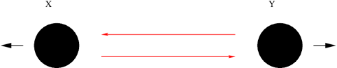
Figure 3: The Dolgov-Novikov time machine proposal. A superluminal signal from $X$, described as backwards-in-time in a relevant frame, is sent towards a second gravitating source $Y$ moving relative to $X$ and returned symmetrically.

They now claim that a superluminal photon emitted with velocity $v(r)$ in the region of $X$ will travel backwards in time (according to the physically relevant coordinate $t^{\prime}$) to a receiver in the region of $Y$. A signal is then returned symmetrically to be received at its original position in the vicinity of $X$, arriving, according to DN, in its past. This would then be analogous to the situation illustrated in Fig. 2.

However, as we emphasised in section 2.1, we are not free to realise the scenario of Fig. 2 in the gravitational case, because the SEP-violating superluminal propagation proposed by Drummond and Hathrell is pre-determined, fixed by the local curvature. The $t^{\prime}$ frame may describe back-in-time motion for the outward leg, but it does not follow that the return path is similarly back-in-time in the same frame. The appropriate special relativistic analogue is the scenario of Fig. 1, not Fig. 2. This critique of the DN time machine proposal has already been made by Konstantinov[18] and further discussion of the related effect in flat spacetime with Casimir plates is given in ref.[12]. The relative motion of the two sources, which at first sight seems to allow the backwards-in-time coordinate $t^{\prime}$ to be relevant and to be used symmetrically, does not in fact alleviate the problem.

The true situation seems rather more to resemble Fig. 4.

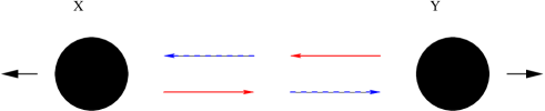
Figure 4: A decomposition of the paths in Fig. 3 for well-separated sources

With the gravitating sources $X$ and $Y$ sufficiently distant that spacetime is separated into regions where it is permissible to neglect one or the other, a signal sent from the vicinity of $X$ towards $Y$ and back would follow the paths shown. But it is clear that this is no more than stitching together an outward plus inward leg near source $X$ with an inward plus outward leg near $Y$. Since both of these are future-directed motions, in the sense of Fig. 1, their combination cannot produce a causality-violating trajectory. If, on the other hand, we consider $X$ and $Y$ to be sufficiently close that this picture breaks down, we lose our ability to analyse the Drummond-Hathrell effect, since we would need the full collision metric for the gravitating sources which is not known for physically realisable examples.

We therefore conclude that the Dolgov-Novikov time machine does not work. The essential idea of trying to realise the causality-violating special relativistic scenario of Fig. 2 by using two gravitational sources in relative motion does not in the end succeed, precisely because the physical Drummond-Hathrell light cones are fixed by the local curvature. Once more it appears that in general relativity with SEP-violating interactions, superluminal photon propagation and causality can be compatible.

2.6 The Event Horizon

We have seen that when quantum effects are taken into account, the physical light cones need not coincide with the geometrical null cones. This immediately raises the question of black hole event horizons – do the physical horizons for light propagation also differ from the geometrical horizons, and are they polarisation dependent? If so, this would have profound repercussions for phenomena such as Hawking radiation.

The answer is best seen using the Newman-Penrose form of the light cone, viz.

$$k^{2}~{}-~{}{(4b+8c)\omega^{2}\over m^{2}}\Phi_{00}~{}~{}\pm~{}~{}{4c\omega^{2}\over m^{2}}(\Psi_{0}+\Psi_{0}^{*})~{}~{}=~{}~{}0$$ (32)

If we define the tetrad with $\ell^{\mu}$ as an outward-directed null vector orthogonal to the horizon 2-surface, then a fundamental theorem on horizons states that both $\Phi_{00}$ and $\Psi_{0}$ are zero precisely at the horizon. The detailed proof, which is given in ref.[19], involves following the convergence and shear of the generators of the horizon. In physical terms, however, it is easily understood as the requirement that the flow of both matter (given by the Ricci term) and gravitational radiation (given by the Weyl term) are zero across the horizon.

It follows that for outward-directed photons with $k_{\mu}=\omega\ell_{\mu}$, the quantum corrections vanish at the horizon and the light cone coincides with the null cone. The geometrical event horizon is indeed the true horizon for physical photon propagation[4, 20]. Again, no conflict arises between superluminal propagation and essential causal properties of spacetime.

3 Causality, Characteristics and the ‘Speeds of Light’

So far, our analysis of photon propagation has been based entirely on the leading-order, Drummond-Hathrell effective action Eq.(1). However, as we show in section 4, the full effective action contains terms to all orders in a derivative expansion and these must be taken into account to go beyond the low-frequency approximation. Photon propagation in QED in curved spacetime is therefore dispersive and we must understand how to identify the ‘speed of light’ which is relevant for causality.

3.1 ‘Speeds of Light’

An illuminating discussion of wave propagation in a simple dispersive medium is given in the classic work by Brillouin[21]. This considers propagation of a sharp-fronted pulse of waves in a medium with a single absorption band, with refractive index $n(\omega)$:

$$n^{2}(\omega)=1-{a^{2}\over\omega^{2}-\omega_{0}^{2}+2i\omega\rho}$$ (33)

where $a,\rho$ are constants and $\omega_{0}$ is the characteristic frequency of the medium. Five distinct velocities are identified: the phase velocity $v_{\rm ph}={\omega\over{|\underline{k}|}}=\Re{1\over n(\omega)}$, group velocity $v_{\rm gp}={d\omega\over d|\underline{k}|}$, signal velocity $v_{\rm sig}$, energy-transfer velocity $v_{\rm en}$ and wavefront velocity $v_{\rm wf}$, with precise definitions related to the behaviour of contours and saddle points in the relevant Fourier integrals in the complex $\omega$-plane. Their frequency dependence is illustrated in Fig. 5.

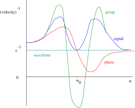
Figure 5: Sketch of the behaviour of the phase, group and signal velocities with frequency in the model described by the refractive index Eq.(33). The energy-transfer velocity (not shown) is always less than $c$ and becomes small near $\omega_{0}$. The wavefront speed is identically equal to $c$.

As the pulse propagates, the first disturbances to arrive are very small amplitude waves, ‘frontrunners’, which define the wavefront velocity $v_{\rm wf}$. These are followed continuously by waves with amplitudes comparable to the initial pulse; the arrival of this part of the complete waveform is identified in ref.[21] as the signal velocity $v_{\rm sig}$. As can be seen from Fig. 5, it essentially coincides with the more familiar group velocity for frequencies far from $\omega_{0}$, but gives a much more intuitively reasonable sense of the propagation of a signal than the group velocity, whose behaviour in the vicinity of an absorption band is relatively eccentric. As the figure makes clear, the phase velocity itself also does not represent a ‘speed of light’ relevant for considerations of signal propagation or causality.

The appropriate velocity to define light cones and causality is in fact the wavefront velocity $v_{\rm wf}$. (Notice that in Fig. 5, $v_{\rm wf}$ is a constant, equal to $c$, independent of the frequency or details of the absorption band.) This is determined by the boundary between the regions of zero and non-zero disturbance (more generally, a discontinuity in the first or higher derivative of the field) as the pulse propagates. Mathematically, this definition of wavefront is identified with the characteristics of the partial differential equation governing the wave propagation[24]. Our problem is therefore to determine the velocity associated with the characteristics of the wave operator derived from the modified Maxwell equations of motion appropriate to the new effective action.

Notice that a very complete and rigorous discussion of the wave equation in curved spacetime has already been given in the monograph by Friedlander[25], in which it is proved (Theorem 3.2.1) that the characteristics are simply the null hypersurfaces of the spacetime manifold, in other words that the wavefront always propagates with the fundamental speed $c$. However, this discussion assumes the standard form of the (gauge-fixed) Maxwell wave equation (cf. ref.[25], eq.(3.2.1)) and does not cover the modified wave equation derived from the action Eq.1, precisely because of the extra curvature couplings which lead to the effective metric $G_{\mu\nu}$ and superluminal propagation.

3.2 Characteristics, Wavefronts and the Phase Velocity $v_{\rm ph}(\infty)$

Instead, the key result which allows a derivation of the wavefront velocity is derived by Leontovich[26]. In this paper, an elegant proof is presented for a very general set of PDEs that the wavefront velocity associated with the characteristics is identical to the $\omega\rightarrow\infty$ limit of the phase velocity, i.e.

$$v_{\rm wf}=\lim_{\omega\rightarrow\infty}{\omega\over|\underline{k}|}=\lim_{\omega\rightarrow\infty}v_{\rm ph}(\omega)$$ (34)

The proof is rather formal, but is of sufficient generality to apply to our discussion of photon propagation using the modified effective action of section 4. We reproduce the essential details below.

The first step is to recognise that any second order PDE can be written as a system of first order PDEs by considering the first derivatives of the field as independent variables. Thus, if for simplicity we consider a general second order wave equation for a field $u(t,x)$ in one space dimension, the system of PDEs we need to solve is

$$a_{ij}{\partial\phi_{j}\over\partial t}+b_{ij}{\partial\phi_{j}\over\partial x}+c_{ij}\phi_{j}~{}=~{}0$$ (35)

where $\phi_{i}=\{u,{\partial u\over\partial t},{\partial u\over\partial x}\}$.

Making the ‘geometric optics’ ansatz

$$\phi_{i}~{}=~{}\varphi_{i}\exp i(wt-kx)$$ (36)

where the frequency-dependent phase velocity is $v_{\rm ph}(k)=\omega(k)/k$, and substituting into Eq.(35) we find

$$\Bigl{(}i\omega a_{ij}-ikb_{ij}+c_{ij}\Bigr{)}\varphi_{j}~{}=~{}0$$ (37)

The condition for a solution,

$${\rm det}\Bigl{[}a_{ij}v_{\rm ph}(k)-b_{ij}-{i\over k}c_{ij}\Bigr{]}~{}=~{}0$$ (38)

then determines the phase velocity.

On the other hand, we need to find the characteristics of Eq.(35), i.e. curves ${\cal C}$ on which Cauchy’s theorem breaks down and the evolution is not uniquely determined by the initial data on ${\cal C}$. The derivatives of the field may be discontinuous across the characteristics and these curves are associated with the wavefronts for the propagation of a sharp-fronted pulse. The corresponding light rays are the ‘bicharacteristics’. (See, for example, ref.[24] chapters 5.1, 6.1 for further discussion.)

We therefore consider a characteristic curve ${\cal C}$ in the $(t,x)$ plane separating regions where $\phi_{i}=0$ (ahead of the wavefront) from $\phi_{i}\neq 0$ (behind the wavefront). At a fixed point $(t_{0},x_{0})$ on ${\cal C}$, the absolute derivative of $\phi_{i}$ along the curve, parametrised as $x(t)$, is just

$${d\phi_{i}\over dt}~{}=~{}{\partial\phi_{i}\over\partial t}\Big{|}_{0}+{\partial\phi_{i}\over\partial x}\Big{|}_{0}{dx\over dt}$$ (39)

where $dx/dt=v_{\rm wf}$ gives the wavefront velocity. Using this to eliminate ${\partial\phi_{i}\over\partial t}$ from the PDE Eq.(35) at $(t_{0},x_{0})$, we find

$$\Bigl{(}-a_{ij}{dx\over dt}+b_{ij}\Bigr{)}{\partial\phi_{j}\over\partial x}\Big{|}_{0}+a_{ij}{d\phi_{j}^{(0)}\over dt}+c_{ij}\phi_{j}^{(0)}~{}=~{}0$$ (40)

Now since ${\cal C}$ is a wavefront, on one side of which $\phi_{i}$ vanishes identically, the second two terms above must be zero. The condition for the remaining equation to have a solution is simply

$${\rm det}\Bigl{[}a_{ij}v_{\rm wf}-b_{ij}\Bigr{]}~{}=~{}0$$ (41)

which determines the wavefront velocity $v_{\rm wf}$. The proof is now evident. Comparing Eqs.(38) and (41), we clearly identify

$$v_{\rm wf}~{}=~{}v_{\rm ph}(k\rightarrow\infty)$$ (42)

The wavefront velocity in a gravitational background is therefore not given a priori by $c$. Taking vacuum polarisation into account, there is no simple non-dispersive medium corresponding to the vacuum of classical Maxwell theory in which the phase velocity represents a true speed of propagation; for QED in curved spacetime, even the vacuum is dispersive. In order to discuss causality, we therefore have to extend the original Drummond-Hathrell results for $v_{\rm ph}(\omega\sim 0)$ to the high frequency limit $v_{\rm ph}(\omega\rightarrow\infty)$, as already emphasised in their original work.

A further subtle question arises if we write the standard dispersion relation for the refractive index $n(\omega)$ in the limit $\omega\rightarrow\infty$:

$$n(\infty)=n(0)-{2\over\pi}\int_{0}^{\infty}{d\omega\over\omega}\Im n(\omega)$$ (43)

For a conventional dispersive medium, $\Im n(\omega)>0$, which implies that $n(\infty)<n(0)$, or equivalently $v_{\rm ph}(\infty)>v_{\rm ph}(0)$. Evidently this is satisfied by Fig. 5. The key question though is whether the usual assumption of positivity of $\Im n(\omega)$ holds in the present situation of the QED vacuum in a gravitational field. If so, then (as already noted in ref.[1]) the superluminal Drummond-Hathrell results for $v_{\rm ph}(0)$ would actually be lower bounds on the all-important wavefront velocity $v_{\rm ph}(\infty)$. However, it is not clear that positivity of $\Im n(\omega)$ holds in the gravitational context. Indeed it has been explicitly criticised by Dolgov and Khriplovich in refs.[27, 28], who point out that since gravity is an inhomogeneous medium in which beam focusing as well as diverging can happen, a growth in amplitude corresponding to $\Im n(\omega)<0$ is possible. The possibility of $v_{\rm ph}(\infty)<v_{\rm ph}(0)$, and in particular $v_{\rm ph}(\infty)=c$, therefore does not seem to be convincingly ruled out by the dispersion relation Eq.(43).

4 Dispersion

After these general considerations, we now return to QED in curved spacetime and use the full effective action to study dispersion and investigate the high-frequency limit.

4.1 Effective Action for Photon-Gravity Interactions

The local effective action in QED to $O(RFF)$ keeping terms of all orders in derivatives is derived in ref.[9]. The result is:

$$\begin{array}[]{rcl}&\\ &\Gamma=\int dx\sqrt{-g}\biggl{[}-{1\over 4}F_{\mu\nu}F^{\mu\nu}~{}+~{}{1\over m^{2}}\Bigl{(}D_{\mu}F^{\mu\l}~{}\overrightarrow{G_{0}}~{}D_{\nu}F^{\nu}{}_{\l}\\[4.0pt] &~{}~{}~{}~{}~{}~{}+~{}\overrightarrow{G_{1}}~{}RF_{\mu\nu}F^{\mu\nu}~{}+~{}\overrightarrow{G_{2}}~{}R_{\mu\nu}F^{\mu\l}F^{\nu}{}_{\l}~{}+~{}\overrightarrow{G_{3}}~{}R_{\mu\nu\l\rho}F^{\mu\nu}F^{\l\rho}\Bigr{)}\\ &~{}+~{}{1\over m^{4}}\Bigl{(}\overrightarrow{G_{4}}~{}RD_{\mu}F^{\mu\l}D_{\nu}F^{\nu}{}_{\l}~{}+~{}\overrightarrow{G_{9}}~{}R_{\mu\nu\l\rho}D_{\sigma}F^{\sigma\rho}D^{\l}F^{\mu\nu}\\ &~{}~{}~{}~{}+~{}\overrightarrow{G_{5}}~{}R_{\mu\nu}D_{\l}F^{\l\mu}D_{\rho}F^{\rho\nu}~{}+~{}\overrightarrow{G_{6}}~{}R_{\mu\nu}D^{\mu}F^{\l\rho}D^{\nu}F_{\l\rho}\\ &~{}~{}~{}~{}~{}~{}~{}~{}~{}~{}+~{}\overrightarrow{G_{7}}~{}R_{\mu\nu}D^{\mu}D^{\nu}F^{\l\rho}F_{\l\rho}~{}+~{}\overrightarrow{G_{8}}~{}R_{\mu\nu}D^{\mu}D^{\l}F_{\l\rho}F^{\rho\nu}~{}\Bigr{)}~{}~{}\biggr{]}\\ &&\end{array}$$ (44)

This was found by adapting a background field action valid to third order in generalised curvatures due to Barvinsky, Gusev, Zhytnikov and Vilkovisky[29] (see also ref.[30]) and involves re-expressing their more general result in manifestly local form by an appropriate choice of basis operators.

In this formula, the $\overrightarrow{G_{n}}$ ($n\geq 1$) are form factor functions of three operators:

$$\overrightarrow{G_{n}}\equiv G_{n}\Bigl{(}{D_{(1)}^{2}\over m^{2}},{D_{(2)}^{2}\over m^{2}},{D_{(3)}^{2}\over m^{2}}\Bigr{)}$$ (45)

where the first entry ($D_{(1)}^{2}$) acts on the first following term (the curvature), etc. $\overrightarrow{G_{0}}$ is similarly defined as a single variable function. These form factors are found using heat kernel methods and are given by ‘proper time’ integrals of known algebraic functions. Their explicit expressions can be found in ref.[9]. Evidently, Eq.(44) reduces to the Drummond-Hathrell action if we neglect all the higher order derivative terms.

4.2 Dispersion and the Light Cone

The next step is to derive the equation of motion analogous to Eq.(11) from this generalised effective action and to apply geometric optics to find the corresponding light cone. This requires a very careful analysis of the relative orders of magnitudes of the various contributions to the equation of motion arising when the factors of $D^{2}$ in the form factors act on the terms of $O(RF)$. These subtleties are explained in detail in ref.[8]. The final result for the new effective light cone has the form

$$k^{2}~{}-~{}{1\over m^{2}}F\Bigl{(}{k.D\over m^{2}}\Bigr{)}R_{\mu\l}k^{\mu}k^{\l}~{}+~{}{1\over m^{2}}G\Bigl{(}{k.D\over m^{2}}\Bigr{)}R_{\mu\nu\l\rho}k^{\mu}k^{\l}a^{\nu}a^{\rho}~{}~{}=~{}~{}0$$ (46)

where $F$ and $G$ are known functions with well-understood asymptotic properties[8]. Clearly, for agreement with Eq.(12), we have $F(0)=2b$, $G(0)=8c$.

The novel feature of this new light cone condition is that $F$ and $G$ are functions of the operator $k.D$ acting on the Ricci and Riemann tensors. So although the asymptotic behaviour of $F$ and $G$ as functions is known, this information is not really useful unless the relevant curvatures are eigenvalues of the operator. On the positive side, however, $k.D$ does have a clear geometrical interpretation – it simply describes the variation along a null geodesic with tangent vector $k^{\mu}$.

The utility of this light cone condition therefore seems to hinge on what we know about the variations along null geodesics of the Ricci and Riemann (or Weyl) tensors. It may therefore be useful to re-express Eq.(46) in Newman-Penrose form:

$$k^{2}~{}-~{}{\omega^{2}\over m^{2}}\tilde{F}\Bigl{(}{\omega\ell.D\over m^{2}}\Bigr{)}\Phi_{00}~{}\pm~{}{\omega^{2}\over 2m^{2}}G\Bigl{(}{\omega\ell.D\over m^{2}}\Bigr{)}(\Psi_{0}+\Psi_{0}^{*})~{}~{}=~{}~{}0$$ (47)

where $\tilde{F}=2F+G$.

Unfortunately, we have been unable to find any results in the relativity literature for $\ell.D\Phi_{00}$ and $\ell.D\Psi_{0}$ which are valid in a general spacetime. In particular, this is not one of the combinations that are constrained by the Bianchi identities in Newman-Penrose form (as displayed for example in ref.[31], chapter 1, Eq.(321)). To try to build some intuition, we have therefore looked at particular cases. The most interesting is the example of photon propagation in the Bondi-Sachs metric[32, 33] which we recently studied in detail[7].

The Bondi-Sachs metric describes the gravitational radiation from an isolated source. The metric is

$$ds^{2}=-Wdu^{2}-2e^{2\beta}dudr+r^{2}h_{ij}(dx^{i}-U^{i}du)(dx^{j}-U^{j}du)$$ (48)

where

$$h_{ij}dx^{i}dx^{j}={1\over 2}(e^{2\gamma}+e^{2\delta})d\theta^{2}+2\sinh(\gamma-\delta)\sin\theta d\theta d\phi+{1\over 2}(e^{-2\gamma}+e^{-2\delta})\sin^{2}\theta d\phi^{2}$$ (49)

The metric is valid in the vicinity of future null infinity ${\cal I}^{+}$. The family of hypersurfaces $u=const$ are null, i.e. $g^{\mu\nu}\partial_{\mu}u\partial_{\nu}u=0$. Their normal vector $\ell_{\mu}$ satisfies

$$\ell_{\mu}=\partial_{\mu}u~{}~{}~{}~{}~{}~{}~{}~{}~{}~{}~{}~{}~{}\Rightarrow~{}~{}~{}~{}~{}\ell^{2}=0,~{}~{}~{}~{}~{}~{}~{}~{}\ell^{\mu}D_{\mu}\ell^{\nu}=0$$ (50)

The curves with tangent vector $\ell^{\mu}$ are therefore null geodesics; the coordinate $r$ is a radial parameter along these rays and is identified as the luminosity distance. The six independent functions $W,\beta,\gamma,\delta,U^{i}$ characterising the metric have expansions in ${1\over r}$ in the asymptotic region near ${\cal I}^{+}$, the coefficients of which describe the various features of the gravitational radiation.

In the low frequency limit, the light cone is given by the simple formula Eq.(4) with $\Phi_{00}=0$. The velocity shift is quite different for the case of outgoing and incoming photons[7]. For outgoing photons, $k^{\mu}=\ell^{\mu}$, and the light cone is

$$k^{2}~{}~{}=~{}~{}\pm~{}{4c\omega^{2}\over m^{2}}~{}\Bigl{(}\Psi_{0}+\Psi_{0}^{*}\Bigr{)}~{}~{}\sim~{}~{}O\Bigl{(}{1\over r^{5}}\Bigr{)}$$ (51)

while for incoming photons, $k^{\mu}=n^{\mu}$,

$$k^{2}~{}~{}=~{}~{}\pm~{}{4c\omega^{2}\over m^{2}}~{}\Bigl{(}\Psi_{4}+\Psi_{4}^{*}\Bigr{)}~{}~{}\sim~{}~{}O\Bigl{(}{1\over r}\Bigr{)}$$ (52)

Now, it is a special feature of the Bondi-Sachs spacetime that the absolute derivatives of each of the Weyl scalars $\Psi_{0},\ldots,\Psi_{4}$ along the ray direction $\ell^{\mu}$ vanishes, i.e. $\Psi_{0},\ldots,\Psi_{4}$ are parallel transported along the rays[33, 34]. In this case, therefore, we have:

$$\ell\cdot D~{}\Psi_{0}~{}=~{}0~{}~{}~{}~{}~{}~{}~{}~{}~{}~{}~{}~{}~{}~{}~{}~{}~{}~{}~{}~{}~{}~{}~{}~{}~{}~{}~{}~{}\ell\cdot D~{}\Psi_{4}~{}=~{}0$$ (53)

but there is no equivalent simple result for either $n\cdot D~{}\Psi_{4}$ or $n\cdot D~{}\Psi_{0}$.

Although it is just a special case, Eq.(53) nevertheless leads to a remarkable conclusion. The full light cone condition Eq.(47) applied to outgoing photons in the Bondi-Sachs spacetime now reduces to

$$k^{2}~{}\pm~{}{\omega^{2}\over 2m^{2}}~{}G\bigl{(}0\bigr{)}\Bigl{(}\Psi_{0}+\Psi_{0}^{*}\Bigr{)}~{}~{}=~{}~{}0$$ (54)

since $\ell\cdot D\Psi_{0}=0$. In other words, the low-frequency Drummond-Hathrell prediction of a superluminal phase velocity $v_{\rm ph}(0)$ is exact for all frequencies. There is no dispersion, and the wavefront velocity $v_{\rm ph}(\infty)$ is indeed superluminal.

This is potentially a very important result. Based on the improved effective action Eq.(44), we have shown there is at least one example in which the wavefront truly propagates with superluminal velocity. Quantum effects have indeed shifted the light cone into the geometrically spacelike region.

4.3 Non-Perturbative Effective Action and High-Frequency Propagation

Unfortunately, there is one final twist to the story which could invalidate the above conclusion. If instead of a gravitational field, we consider photon propagation in a constant background magnetic field, we find the following birefringent modification to the light cones:[35, 36, 8]

$$k^{2}~{}~{}-~{}~{}{\alpha\over 2\pi}\Bigl{(}{eB\omega\over m^{2}}\Bigr{)}^{2}~{}\int_{-1}^{1}du\int_{0}^{\infty}ds~{}s~{}N_{\parallel,\perp}(u,z)~{}e^{-is\bigl{(}1+s^{2}\Omega^{2}P(u,z)\bigr{)}}~{}~{}=~{}~{}0$$ (55)

where $z={eB\over m^{2}}s$ and $\Omega={eB\over m^{2}}{\omega\over m}$. Exact expressions are known for the functions $N$ and $P$ as well as their weak-field expansions.

Now, in the weak-field, low-frequency regime, $\Omega\ll 1$ and we can simply expand the exponential to leading order in $\Omega^{2}P$. The low-frequency limit of the phase velocity for the two polarisations is the well-known result[2, 37]

$$v_{\rm ph}(0)~{}~{}=~{}~{}1-{\alpha\over 4\pi}\Bigl{(}{eB\over m^{2}}\Bigr{)}^{2}~{}\Bigl{[}{14\over 45}_{\parallel},{8\over 45}_{\perp}\Bigr{]}$$ (56)

and is in each case subluminal. At high frequencies, however, Eq.(55) is dominated by the rapidly-varying phase factor $\exp(-is^{3}\Omega^{2}P)$ and the correction to the phase velocity tends to zero (from a superluminal value) with a non-analytic $\Omega^{-{4/3}}$ behaviour:

$$v_{\rm ph}(\omega\rightarrow\infty)~{}~{}=~{}~{}1+{\alpha\over 4\pi}\Bigl{(}{eB\over m^{2}}\Bigr{)}^{2}~{}\bigl{[}{c}_{\parallel},{c}_{\perp}\bigr{]}~{}\Omega^{-{4\over 3}}$$ (57)

where ${c}_{\parallel},{c}_{\perp}$ are known positive constants[8]. The phase velocity therefore has the standard form for a dispersive medium illustrated in Fig. 5. In particular, the wavefront velocity $v_{\rm wf}=v_{\rm ph}(\infty)=c$.

The important lesson for the gravitational case is this. If we had simply used an effective action for QED in a background electromagnetic field keeping terms up to $O(F^{4})$ in the field strength and to all orders in derivatives, generalising the Euler-Heisenberg Lagrangian, we would have accurately found the leading low-frequency dependence of $v_{\rm ph}(\omega)$ but would have completely missed the non-analytic high-frequency behaviour. This arises from terms in the full effective action which are non-perturbative in the background field and give rise to the phase factor in Eq.(55).

If the gravitational case is similar, this would imply that the modified light cone can be written heuristically as

$$k^{2}~{}+~{}{\alpha\over\pi}\int_{0}^{\infty}ds~{}{\cal N}(s,R)~{}e^{-is\bigl{(}1+s^{2}\Omega^{2}{\cal P}(s,R)\bigr{)}}~{}~{}=~{}~{}0$$ (58)

where both ${\cal N}$ and ${\cal P}$ can be expanded in powers of curvature, and derivatives of curvature, presumably associated with factors of $\omega$ as in the last section. The frequency dependent factor $\Omega$ would be $\Omega\sim{R\over m^{2}}{\omega\over m}\sim O({\l_{c}^{3}\over\l L^{2}})$, where ‘$R$’ denotes some generic curvature component and $L$ is the typical curvature scale. If this is true, then an expansion of the effective action to $O(RFF)$, even including higher derivatives, would not be sufficient to reproduce the full, non-perturbative contribution $\exp(-is^{3}\Omega^{2}{\cal P})$. The Drummond-Hathrell action would correspond to the leading order term in the expansion of Eq.(58) in powers of ${R\over m^{2}}$ neglecting derivatives, while our improved effective action of section 4.1 sums up all orders in derivatives while retaining the restriction to leading order in curvature.

The omission of the non-perturbative contribution would be justified only in the limit of small $\Omega$, i.e. for ${\l_{c}^{3}\over\l L^{2}}\ll 1$. Neglecting this therefore prevents us from accessing the genuinely high frequency limit $\l\rightarrow 0$ needed to find the asymptotic limit $v_{\rm ph}(\infty)$ of the phase velocity. Moreover, assuming Eq.(58) is indeed on the right lines, it also seems inevitable that for high frequencies (large $\Omega$) the rapid phase variation in the exponent will drive the entire heat kernel integral to zero, ensuring the wavefront velocity $v_{\rm wf}=c$.

4.4 Outlook

At present, it is not clear how to make further progress. The quantum field theoretic calculation required to find such non-perturbative contributions to the effective action and confirm an $\exp(-is^{3}\Omega^{2}{\cal P})$ structure in Eq.(58) appears difficult, although some technical progress in this area has been made recently in ref.[38] and work in progress[39]. One of the main difficulties is that since a superluminal effect requires some anisotropy in the curvature, it is not sufficient just to consider constant curvature spacetimes. (Recall that the Ricci scalar term in the effective action Eq.(1) does not contribute to the modified light cone Eq.(2).) A possible approach to this problem, which would help to control the plethora of indices associated with the curvatures, might be to reformulate the heat kernel calculations directly in the Newman-Penrose basis. On the other hand, perhaps a less ambitious goal would be to try to determine just the asymptotic form of the non-perturbative contribution in the $\Omega\rightarrow\infty$ limit.

A final resolution of the dispersion problem for QED in curved spacetime has therefore still to be found. If the perturbative expansion of the effective action to $O(RFF)$ is sufficient, then as we have seen there exist at least some examples where the wavefront velocity is really superluminal. In this case, all the issues concerning causality discussed in section 2 would apply to QED. Perhaps more likely, however, is the scenario described above, where the high-frequency dispersion is driven by non-perturbative contributions to the effective action such that the wavefront velocity remains precisely $c$. It would then be interesting to see exactly how the phase velocity behaves as a function of $\omega$ (c.f. Fig. 5) and whether the explanation advanced in section 3.2 for the non-validity of the standard refractive index dispersion relation Eq.(43) is correct.

Finally, of course, even if it does turn out that $v_{\rm wf}=c$ for QED itself, the discussion of causality in this paper may still be relevant to photon propagation in more speculative theories, including bimetric theories of gravity[14], string-inspired non-linear electrodynamics[20], Lorentz and CPT violating effective Lagrangians[40] and non-commutative gauge theories.

References

- [1] I.T. Drummond and S. Hathrell, Phys. Rev. D22 (1980) 343.
- [2] R.D. Daniels and G.M. Shore, Nucl. Phys. B425 (1994) 634.
- [3] J. I. Latorre, P. Pascual and R. Tarrach, Nucl. Phys. B437 (1995) 60.
- [4] G.M. Shore, Nucl. Phys. B460 (1996) 379.
- [5] W. Dittrich and H. Gies, Phys. Lett. B431 (1998) 420-429; Phys. Rev. D58 (1998) 025004.
- [6] R.D. Daniels and G.M. Shore, Phys. Lett. B367 (1996) 75.
- [7] G.M. Shore, Nucl. Phys. B605 (2001) 455.
- [8] G.M. Shore, Nucl. Phys. B633 (2002) 271.
- [9] G.M. Shore, Nucl. Phys. B646 (2002) 281.
- [10] K. Scharnhorst, Phys. Lett. B236 (1990) 354.
- [11] G. Barton, Phys. Lett. B237 (1990) 559.
- [12] S. Liberati, S. Sonego and M. Visser, Annals Phys. 298 (2002) 167.
- [13] S.W. Hawking and G.F.R. Ellis, The Large Scale Structure of Spacetime, Cambridge University Press, 1973.
- [14] I.T. Drummond, Phys. Rev. D63 (2001) 043503.
- [15] A.D. Dolgov and I.D. Novikov, Phys. Lett. B442 (1998) 82.
- [16] J.R. Gott, Astrophys. J. 288 (1985) 422.
- [17] G.M. Shore, gr-qc/0210048, to be published in Int. J. Mod. Phys. A
- [18] M.Yu. Konstantinov, gr-qc/9810019; Russ. Phys. J. 45 (2002) 23.
- [19] S.W. Hawking, ‘The Event Horizon’, 1972 Les Houches lectures, ed. B. De Witt, Gordon and Breach, 1972.
- [20] G.W. Gibbons and C.A.R. Herdeiro, Phys. Rev. D63 (2001) 064006.
- [21] L. Brillouin, Wave Propagation and Group Velocity, Academic Press (London) 1960.
- [22] L.V. Hau, Scientific American 7 (2001) 66.
- [23] L.J. Wang, A. Kuzmich and A. Dogoriu, Nature 406 (2000) 277.
- [24] R. Courant and D. Hilbert, Methods of Mathematical Physics, Vol II, Interscience, New York, 1962.
- [25] F.G. Friedlander, The Wave Equation on a Curved Spacetime, Cambridge University Press, 1975.
- [26] M.A. Leontovich, in L.I. Mandelshtam, Lectures in Optics, Relativity and Quantum Mechanics, Nauka, Moscow 1972 (in Russian).
- [27] A.D. Dolgov and I.B. Khriplovich, Sov. Phys. JETP 58(4) (1983) 671.
- [28] I.B. Khriplovich, Phys. Lett. B346 (1995) 251.
- [29] A.O. Barvinsky, Yu.V. Gusev, G.A. Vilkovisky and V.V. Zhytnikov, Print-93-0274 (Manitoba), 1993.
- [30] A.O. Barvinsky, Yu.V. Gusev, G.A. Vilkovisky and V.V. Zhytnikov, J. Math. Phys. 35 (1994) 3525; J. Math. Phys. 35 (1994) 3543; Nucl. Phys. B439 (1995) 561.
- [31] S. Chandresekhar, The Mathematical Theory of Black Holes, Clarendon, Oxford, 1985.
- [32] H. Bondi, M.G.J. van der Burg and A.W.K. Metzner, Proc. Roy. Soc. A269 (1962) 21
- [33] R.K. Sachs, Proc. Roy. Soc. A270 (1962) 103.
- [34] R.A. d’Inverno, Introducing Einstein’s Relativity, Clarendon, Oxford, 1992.
- [35] W. Tsai and T. Erber, Phys. Rev. D10 (1974) 492.
- [36] W. Tsai and T. Erber, Phys. Rev. D12 (1975) 1132.
- [37] S. Adler, Ann. Phys. (N.Y.) 67 (1971) 599.
- [38] A.O. Barvinsky and V.F. Mukhanov, Phys. Rev. D66 (2002) 065007.
- [39] Yu.V. Gusev, private communication.
- [40] V.A. Kostelecky, Phys. Rev. D58 (1998) 116002.