Attractor Phantom Solution

Abstract

ABSTRACT: In light of recent study on the dark energy models that manifest an equation of state $w<-1$, we investigate the cosmological evolution of such a phantom field in a specific potential, exponential potential in this paper. The phase plane analysis show that the there is a late time attractor solution in this model, which address the similar issues as that of fine tuning problems in conventional quintessence models. The equation of state $w$ is determined by the attractor which is dependent on the $\lambda$ parameter in the potential. We also show that this model is stable for our present observable Universe.

1. Introduction

Recent observation shows that our universe is made up of roughly two third of dark energy that has negative pressure and can drive the accelerating expansion of the universenewobservation . Present data from the observation allows the equation of state in the range $-1.62<w<-0.74$melchiorri . However, the equation of state of conventional quintessence modelssteinhardt that based on a scalar field and positive kinetic energy can not evolve to the the regime of $w<-1$. Some authorscaldwell1 ; sahni ; parker ; chiba ; boisseau ; schulz ; faraoni ; maor ; onemli ; torres ; carroll ; frampton ; caldwell2 ; gibbons investigated a phantom field model which has negative kinetic energy and can realize the $w<-1$ in its evolution. Although the introduction of a phantom field causes many theoretical problems such as the violation of some widely accepted energy condition and the rapid vacuum decaycarroll , it is still very interesting in the sense that it can fit current observations well. Comparing with other approaches to realizing the $w<-1$, such as the modification of Friedman equation, it seems more economical.

In this paper, provisionally leaving aside the theoretical puzzles about phantom field, we study the detailed evolution of the phantom field and the attractor property of its solution via a specific model. by using the qualitative approach to the dynamical system, phase plane analysis, we prove the existence of a late time attractor solution, at which the phantom become dominant and the equation of state is freezed with only small oscillation. Exponential potentials attract much attention because they can be derived from the effective interaction in string theory, higher dimensional gravity and the non-perturbative effects such as gaugino condensationstring and their roles in cosmological context have also been widely investigatedlucchin . We therefore consider the phantom evolution in exponential potential in the following.

2. Phantom in Exponential Potential

In the spatially flat Robertson-Walker metric,

$$ds^{2}=dt^{2}-a^{2}(t)(dx^{2}+dy^{2}+dz^{2})$$ (1)

The Lagrangian density for the spatially homogeneous phantom field is

$$L_{\Phi}=-\frac{1}{2}g^{\mu\nu}(\partial_{\mu}\phi)(\partial_{\nu}\phi)-V(\phi)$$ (2)

when consider the presence of baryotropic fluid, the action for the model is

$$S=\int d^{4}x\sqrt{-g}(-\frac{1}{2\kappa^{2}}R_{s}-p_{\gamma}+L_{\phi})$$ (3)

where $g$ is the determinant of the metric tensor $g_{\mu\nu}$, $\kappa^{2}=8\pi G$, $R_{s}$ is the Ricci scalar,and $\rho_{\gamma}$ is the density of fluid with a baryotropic equation of state $p_{\gamma}=(\gamma-1)\rho_{\gamma}$, where $0\leq\gamma\leq 2$ is a constant that relates to the equation of state by $w=\gamma-1$. By varying the action, one can obtain the Einstein equations and the equations of motion for the scalar field as

$$\dot{H}=-\frac{\kappa^{2}}{2}(\rho_{\gamma}+p_{\gamma}-\dot{\phi}^{2})$$ (4)

$$\dot{\rho_{\gamma}}=-3H(\rho_{\gamma}+p_{\gamma})$$ (5)

$$\ddot{\phi}+3H\dot{\phi}+\lambda\kappa V(\phi)=0$$ (6)

$$H^{2}=\frac{\kappa^{2}}{3}[\rho_{\gamma}+\rho_{\Phi}]$$ (7)

where

$$\rho_{\Phi}=-\frac{1}{2}\dot{\phi}^{2}+V(\phi)$$ (8)

$$p_{\Phi}=-\frac{1}{2}\dot{\phi}^{2}-V(\phi)$$ (9)

are the energy density and pressure of the $\Phi$ field respectively , and $H$ is Hubble parameter. The potential $V(\phi)$ is exponentially dependent on $\phi$ as $V(\phi)=V_{0}\exp(-\lambda\kappa\phi)$.The equation-of-state parameter for the phantom is

$$w=\frac{p_{\Phi}}{\rho_{\Phi}}=\frac{\dot{\phi}^{2}+2V(\phi)}{\dot{\phi}^{2}-2V(\phi)}$$ (10)

It is clear that the phantom field could realize the equation of state $w<-1$ when

$$0<\dot{\phi}^{2}<2V(\phi)$$ (11)

3. Attractor Solution of Phantom Model

In this section, we investigate the global structure of the dynamical system via phase plane analysis and compute the cosmological evolution by numerical analysis. Introduce the following variables

$$x= \frac{\kappa}{\sqrt{6}H}\dot{R}$$ (12)

$$y= \frac{\kappa\sqrt{V(R)}}{\sqrt{3}H}$$

$$N= \log a$$

the equation system(4-7) could be reexpressed as the following autonomous system:

$$\frac{dx}{dN}=\frac{3}{2}x[\gamma(1+x^{2}-y^{2})-2x^{2}]-(3x+\sqrt{\frac{3}{2}}\lambda y^{2})$$ (13)

$$\frac{dy}{dN}=\frac{3}{2}y[\gamma(1+x^{2}-y^{2})-2x^{2}]-\sqrt{\frac{3}{2}}\lambda xy$$ (14)

Also, we have a constraint equation

$$\Omega_{\phi}+\frac{\kappa^{2}\rho_{\gamma}}{3H^{2}}=1$$ (15)

where

$$\Omega_{\phi}=\frac{\kappa^{2}\rho_{\phi}}{3H^{2}}=y^{2}-x^{2}$$ (16)

The equation of state for the scalar fields could be expressed in term of the new variables as

$$w_{\phi}=\frac{P_{\phi}}{\rho_{\phi}}=\frac{x^{2}+y^{2}}{x^{2}-y^{2}}$$ (17)

It is not difficult to find the physically meaningful critical points $(x_{c},y_{c})$ are $(0,0)$ and $(-\frac{\lambda}{\sqrt{6}},\sqrt{1+\frac{\lambda^{2}}{6}})$. To gain some insight into the property of the critical points, we write the variables near the critical points $(x_{c},y_{c})$ in the form

$$x=x_{c}+u$$ (18)

$$y=y_{c}+v$$

where $u,v$ are perturbations of the variables near the critical points. Substitute the expression (18) into the autonomous system (4-7), one can obtain the equations for the linear perturbations up to the first order as following:

$$\frac{du}{dN}=M_{11}u+M_{12}v$$ (19)

$$\frac{du}{dN}=M_{21}u+M_{22}v$$

The coefficients of the perturbation equations form a $2\times 2$ matrix $M$ whose eigenvalues determine the type and stability of the critical points. One can easily find that the eigenvalues of $M$ for $(0,0)$ is $(\frac{3}{2}(-2+\gamma),\frac{3\gamma}{2})$ and those for $(-\frac{\lambda}{\sqrt{6}},\sqrt{1+\frac{\lambda^{2}}{6}})$ is $(-3-\frac{\lambda^{2}}{2},-3\gamma-\lambda^{2})$. Therefore, point (0,0) is a saddle point while $(-\frac{\lambda}{\sqrt{6}},\sqrt{1+\frac{\lambda^{2}}{6}})$ is a stable node, which corresponds to an attractor solution. At this attractor solution, from Eq.(16, 17 ), we know that $\Omega_{\phi}=1$ and $w_{\phi}=-1-\frac{\lambda^{2}}{3}$, which indicate the phantom domination and the possibility of $w<-1$.

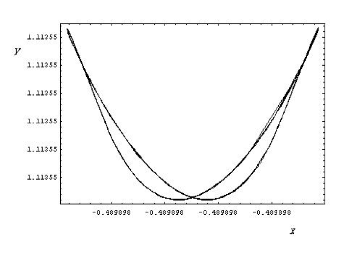
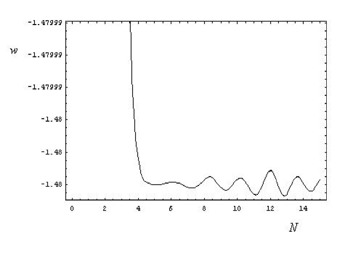
Figure 1: the phase graph of $y$ to $x$

Figure 2: The evolution of Equation of state of Phantom $w$ with respect to $N$

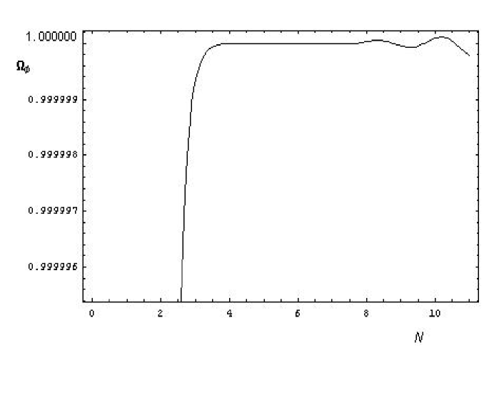
Figure 3: The evolution of $\Omega_{\phi}$ with respect to $N$

Next, we study the system by numerical analysis. The results are in Fig.1, Fig.2 and Fig.3. The computation was done at $\lambda=1.2$ and $\gamma=1.0$. From the figures, we can find that the attractor property of the solution and the phantom field will slightly oscillate around the fixed point at late time and the equation of state is smaller than $-1$.

4. Discussion

We studied a specific phantom model and show that there exists a late time attractor solution in the evolution of the field. The late time attractor solution corresponds to the phantom dominate phase and the equation of state could be smaller than $-1$. This is a very interesting feature of the model we considered here. Now, we consider the stability of the phantom field under perturbation in such a potential. The perturbed metric in synchronous gauge could be expressed ascaldwell1 ; carroll

$$ds^{2}=dt^{2}-a^{2}(t)(\delta_{ij}-h_{ij})dx^{i}dx^{j}$$ (20)

Then, a Fourier mode of the phantom field

$$\delta\phi(t,\textbf{k})=\frac{1}{\sqrt{2\pi}}\int\delta\phi(t,\textbf{x})e^{-i\textbf{k}\cdot\textbf{x}}d^{3}x$$ (21)

satisfies the equation of motion

$$\delta\ddot{\phi_{k}}+3H\delta\dot{\phi_{k}}+(k^{2}-V"(\phi))=-\frac{1}{2}\dot{h}\dot{\phi}$$ (22)

where the $h$ is the trace of $h_{ij}$ and the prime denote the derivative with respect to $\phi$. The effective mass for the perturbation is $[k^{2}-V"(\phi)]^{1/2}$. When the potential is chosen as the exponential $V(\phi)=V_{0}\exp(-\lambda\kappa\phi)$, we have $[k^{2}-\lambda^{2}\kappa^{2}V_{0}\exp(-\lambda\kappa\phi)]^{1/2}$. When the field evolves to its stable attractor solution, the cutoff wave number of the perturbation should be

$$k<\lambda H\sqrt{3+\frac{\lambda^{2}}{2}}$$ (23)

so that the instability does not appear. Surely, it is not to say that the instability will not appear during the evolution before the field reaches the attractor. Since we do not know what will be the specific evolution track the field took in the past, we can only say that at present situation, which is the attractor solution epoch, the perturbation should not violate Eq.(23) to safeguard the stability of the phantom field. Another remarkable feature of such an model is that the evolution of field is toward to its attractor no matter what is its initial value. Since $w_{\phi}=-1-\frac{\lambda^{2}}{3}$, it is determined by the parameter $\lambda$ of the potential and is independent of the choice of the initial value of the field, which make the fine tuning of the field unnecessary.

ACKNOWLEDGEMENT: This work was partially supported by National Nature Science Foundation of China under Grant No. 19875016, National Doctor Foundation of China under Grant No. 1999025110, and Foundation of Shanghai Development for Science and Technology under Grant No.01JC14035.

References

- (1) P de Bernardis et al 2000 Nature 404 955; S Hanany et al 2000 Astrophys. J. 545 1; N Bahcall, J P Ostriker, S Perlmutter and P J Steinhardt 1999 Science 284 1481; S Perlmutter et al 1999 Astrophys. J. 517 565; A G Riess et al 1998 Astron. J. 116 1009
- (2) A. Melchiorri, L. Mersini, C. J. Odmann and M. Trodden, Astro-ph/0211522
- (3) B. Ratra and P. J. Peebles, Phys. Rev. D373406(1988); R. R. Caldwell, R. Dave and P. J. Steinhardt, Phys. Rev. Lett. 801582(1998); P. J. Steinhardt, L . Wang and I . Zlatev, Phys. Rev. D59123504(1999); I. Zlatev, L. Wang and P. J. Steinhardt, Phys. Rev. Lett. 82896(1999); K. Coble, S. Dodelson, J. Frieman, Phys. Rev. D551851(1997); X. Z. Li, J. G. Hao, D. J. Liu, Class.Quant.Grav. 19 (2002) 6049-6058
- (4) R.R. Caldwell, Phys.Lett. B54523-29(2002).
- (5) V. Sahni and A. A. Starobinsky, Int. J. Mod. Phys. D9,373(2002)
- (6) L. Parker and A. Raval, Phys. Rev. D60, 063512(1999)
- (7) T. Chiba, T. Okabe and M. Yamaguchi, Phys. Rev. D62, 023511(2000)
- (8) B. Boisseau, G. Esposito-Farese, D. Polarski and A. A. Starobinsky, Phys. Rev. Lett.85, 2236, (2000)
- (9) A. E. Schulz, Martin White, Phys.Rev. D64 (2001) 043514
- (10) V. Faraoni, Int. J. Mod. Phys. D64, 043514 (2002)
- (11) I. Maor, R. Brustein, J. Mcmahon and P. J. Steinhardt, Phys. Rev. D65 123003(2002)
- (12) V. K. Onemli and R. P. Woodard, Class. Quant. Grav. 19, 4607(2002)
- (13) D. F. Torres, Phys. Rev. D66, 043522 (2002)
- (14) S. M. Carroll, M. Hoffman, M. Trodden, Can the dark energy equation-of-state parameter w be less than -1?, astro-ph/0301273
- (15) P. H. Frampton, Stability Issues for Dark Energy, hep-th/0302007
- (16) R. R Caldwell, M. Kamionkowski and N. N. Weinberg, Phantom energy and cosmic doomsday, astro-ph/0302506
- (17) G. W. Gibbons, Phantom matter and the cosmological constant, hep-th/0302199
- (18) M. B. Green, J. H. Schwarz, and E. Witten, Superstring theory(Cambridge University Press, Cambridge, England,1987)
- (19) F. Lucchin and S. Matarrese, Phys. Rev. D32, 1316(1985); Y. Kitada and K. Maeda, Class. Quantum Grav. 10, 703(1993); E. J. Copeland, A. R. Liddle and D. Wands, Phys. Rev. D57(1998)4686