Exact vacuum solution of a $(1+2)$–dimensional Poincaré gauge theory: BTZ solution with torsion

Abstract

In the framework of (1+2)–dimensional Poincaré gauge gravity, we start from the Lagrangian of the Mielke–Baekler (MB) model that depends on torsion and curvature and includes translational and Lorentzian Chern–Simons terms. We find a general stationary circularly symmetric vacuum solution of the field equations. We determine the properties of this solution, in particular its mass and its angular momentum. For vanishing torsion, we recover the BTZ–solution. We also derive the general conformally flat vacuum solution with torsion. In this framework, we discuss Cartan’s (3–dimensional) spiral staircase and find that it is not only a special case of our new vacuum solution, but can alternatively be understood as a solution of the 3–dimensional Einstein–Cartan theory with matter of constant pressure and constant torque. file 3dexact19.tex, 2003-06-21

I Introduction

On first sight, $(1+2)$–dimensional gravity seems to be rather boring. In 3 dimensions (3D), the Weyl tensor vanishes and the curvature is fully determined by the Ricci tensor and thus, via the Einstein equation, by the energy-momentum alone. Outside the sources the curvature is zero and there are no propagating degrees of freedom, i.e., no gravitational waves. Moreover, there is no Newtonian limit. But even if spacetime is flat, it is not trivial globally. A point particle, e.g., generates the spacetime geometry of a cone. In such a geometry we have light bending, double images, etc. The spacetimes for N particles can be constructed similarly by gluing together patches of $(1+2)$D Minkowski space. This was occasionally investigated since the late 1950s, see Deser et al. deser84 and the review of Carlip Carlip98 .

Some problems in $(1+3)$D gravity reduce to an effective ($1+2$)D theory, like the cosmic string, e.g.; the high–temperature behavior of ($1+3$)D theories also motivates the study of $(1+2)$D theories. In this context, Deser, Jackiw, and Tempelton (DJT) proposed a $(1+2)$D gravitational gauge model with topologically generated mass deser82 . However, the real push for $(1+2)$D gravitational models came when Witten formulated the $(1+2)$D Einstein theory as a Chern–Simons theory, in a similar way as proposed by Achúcarro and Townsend amat , and showed its exact solvability in terms of a finite number of degrees of freedom witten88 ; witten89 . Also de Sitter gravity, conformal gravity, and supergravity, in $(1+2)$D, turn out to be equivalent to Chern–Simons theories horne89 ; koehler90 ; dereli00 ; DereliS , see also the recent monograph of Blagojević blagojevic .

Mielke and Baekler (MB) proposed a $(1+2)$D topological gauge model with torsion and curvature mielke91 ; baekler92 from which the DJT–model can be derived by imposing the constraint of vanishing torsion by means of a Lagrange multiplier term. Gravitational theories in $(1+2)$D with torsion, see also Tresguerres tresguerres92 and Kawai kawai94 , are analogous to the continuum theory of lattice defects in crystal physics, in particular, the corresponding theory of dislocations relates to a torsion of the underlying continuum, see Kröner kroener81 , Kleinert kleinert , Dereli and Verçin dereli87 ; dereli91 , Katanaev and Volovich katanaev91 , and Kohler kohler95 . The fresh approach of Lazar lazar00 ; lazar02_1 ; lazar02_2 promises additional insight.

The next important impact on $(1+2)$D gravity was the discovery of a black hole solution by Bañados, Teitelboim, and Zanelli (BTZ) banados92 . The BTZ black hole is locally isometric to anti-de Sitter (AdS) spacetime. It can be obtained, see Brill brill , from the AdS spacetime as a quotient of the latter with the group of finite isometries. It is asymptotically anti–de Sitter and has no curvature singularity at the origin. Nevertheless, it is clearly a black hole: it has an event horizon and, in the rotating case, an inner horizon. Also electrically and magnetically charged generalizations are known. For extensive discussions see the reviews banados93 ; carlip95_1 ; carlip95_2 ; Carlip98 ; banados99 ; birmingham01 . The relevance to $(1+3)$D gravity can also be seen from the fact that the BTZ solution can be derived from the $(1+3)$D Plebański–Carter metric by means of a dimensional reduction procedure, see Cataldo et al. cataldo00 . By means of the BTZ solution, many interesting questions can be addressed in the context of quantum gravity. For example, Strominger computed the entropy of the BTZ black hole microscopically strominger98 . There is also a relationship between the BTZ black hole and string theory, see Hemming and Keski–Vakkuri hemming01 .

Thus, although $(1+2)$D gravity lacks many important features of real, $(1+3)$D gravity, it keeps enough characteristic structure to be of interest, especially in view of the fact that in the $(1+2)$D case many calculations can be done which are far too involved in $(1+3)$D for the time being.

In this paper we show that the BTZ-metric can be embedded in the framework of the specific Poincaré gauge model proposed by Mielke and Baekler. We arrive at a “BTZ-solution with torsion”, see Table 1, and discuss some of its characteristic properties.—

In section II, we introduce briefly the MB–model and its field equations. In vacuum, these yield constant torsion and constant curvature and, by a suitable ansatz, we obtain the new solution displayed in Table 1. In section III, we discuss some of the properties of our new solution. In particular, we compute its quasi–local energy and angular momentum expressions as it was suggested to us by Nester, Chen, Tung, and Wu chen94 ; chen99 ; chen00 ; nester00 ; wu01 ; wu03 .

In section IV we derive the general conformally flat vacuum solution and show its relation to the solution of Table 1. In the final section V, we point out that Cartan’s spiral staircase, an example of a simple non–Euclidean connection that is constructed from 3D Euclidean space, can be understood as a specific vacuum solution of the MB-model as well as a solution of 3D Einstein–Cartan theory with matter of constant pressure and constant torque.

II Mielke-Baekler model and its BTZ-like exact solution

Our geometric arena is 3D Riemann-Cartan space. The basic variables are the coframe $\vartheta^{\alpha}=e_{i}{}^{\alpha}\,dx^{i}$ and the Lorentz connection $\Gamma^{\alpha\beta}=\Gamma_{i}{}^{\alpha\beta}\,dx^{i}$. Latin letters $i,j,\,\dots=0,1,2$ denote holonomic or coordinate indices and Greek letters $\alpha,\beta,\,\dots=\hat{0},\hat{1},\hat{2}$ anholonomic or frame indices. In an orthonormal coframe, which we assume for the rest of our article, the metric is given by $g=-\vartheta^{\hat{0}}\otimes\vartheta^{\hat{0}}+\vartheta^{\hat{1}}\otimes\vartheta^{\hat{1}}+\vartheta^{\hat{2}}\otimes\vartheta^{\hat{2}}$. In such an orthonormal coframe, the connection is antisymmetric $\Gamma^{\alpha\beta}=-\Gamma^{\beta\alpha}$. The frame dual to the coframe reads $e_{\alpha}=e^{i}{}_{\alpha}\,\partial_{i}$, with $e_{\alpha}\rfloor\vartheta^{\beta}=\delta_{\alpha}^{\beta}$, where $\rfloor$ denotes the interior product. We introduce the abbreviation $\vartheta^{\alpha\beta\dots}:=\vartheta^{\alpha}\wedge\vartheta^{\beta}\wedge\cdots$ and the $\eta$-basis (^⋆ denotes the Hodge-star operator) $\eta:={}^{\star}1\,,\quad\eta_{\alpha}:={}^{\star}\vartheta_{\alpha}\,,\quad\eta_{\alpha\beta}:={}^{\star}\vartheta_{\alpha\beta}\,,\quad\eta_{\alpha\beta\gamma}:={}^{\star}\vartheta_{\alpha\beta\gamma}\,.$ In 3 dimensions, $\eta_{\alpha\beta\gamma}$ is the totally antisymmetric unit tensor. For our conventions, one should compare hehl95 .

From the gauge potentials coframe and connection, we can derive the field strengths torsion and curvature ($D$ denotes the exterior covariant derivative),

$$T^{\alpha}:=D\vartheta^{\alpha}=d\vartheta^{\alpha}+\Gamma_{\beta}{}^{\alpha}\wedge\vartheta^{\beta}\,,\quad R_{\alpha}{}^{\beta}:=d\Gamma_{\alpha}{}^{\beta}-\Gamma_{\alpha}{}^{\gamma}\wedge\Gamma_{\gamma}{}^{\beta}\,.$$ (1)

In a Riemann-Cartan space, the connection can be expressed in terms of the torsion and the anholonomity 2-form $\Omega^{\alpha}:=d\vartheta^{\alpha}$,

$$\Gamma_{\alpha\beta}=e_{[\alpha}\rfloor\Omega_{\beta]}-\frac{1}{2}\,\left(e_{\alpha}\rfloor e_{\beta}\rfloor\Omega_{\gamma}\right)\,\vartheta^{\gamma}-e_{[\alpha}\rfloor T_{\beta]}+\frac{1}{2}\,\left(e_{\alpha}\rfloor e_{\beta}\rfloor T_{\gamma}\right)\vartheta^{\gamma}\,,$$

see hehl95 Eq.(3.10.6), for $dg_{\alpha\beta}=0$ and $Q_{\alpha\beta}=0$.

Mielke and Baekler mielke91 ; baekler92 considered the following Lagrangian:

$$V_{\rm MB} = -\frac{\chi}{2\ell}\,R^{\alpha\beta}\wedge\eta_{\alpha\beta}-\frac{\Lambda}{\ell}\,\eta+\frac{\theta_{{\rm T}}}{2\ell^{2}}\,\vartheta^{\alpha}\wedge T_{\alpha}$$ (2)

$$-\frac{\theta_{{\rm L}}}{2}\,\left(\Gamma_{\alpha}{}^{\beta}\wedge d\Gamma_{\beta}{}^{\alpha}-\frac{2}{3}\,\Gamma_{\alpha}{}^{\beta}\wedge\Gamma_{\beta}{}^{\gamma}\wedge\Gamma_{\gamma}{}^{\alpha}\right)+L_{\rm mat}\,.$$

The first term, the usual Einstein-Cartan term, is followed by the cosmological term and the Chern-Simons terms for torsion and curvature, see hehl91 . The last term denotes the matter Lagrangian that is minimally coupled to gravity. The 3D gravitational constant $\ell$ guarantees dimensional consistency. The Einstein-Cartan piece is multiplied by a dimensionless constant $\chi$, with $\chi=1$ or $\chi=0$, and the Chern-Simons pieces by the dimensionless “vacuum angles” $\theta_{\rm T}$ and $\theta_{\rm L}$.

From this model we can derive the Deser-Jackiw-Tempelton (DJT) model of topological massive gravity deser82 by adding a Lagrange multiplier term $\lambda_{\alpha}\,T^{\alpha}$ to the Lagrangian $V_{\rm MB}$ thereby enforcing vanishing torsion. Quite recently, Blagojević and Vasilić blagojevic03 considered a restricted MB-model with $\theta^{2}_{\rm T}+\chi\Lambda\ell^{2}=0$, $\,\theta_{\rm L}=0$, and $\chi=1$, which yields, in vacuum, the field equation $R^{\alpha\beta}=0$, i.e., vanishing curvature, introducing thereby the teleparallel geometry of empty spacetime dynamically. A similar teleparallel model (including torsion square terms) was developed by Sousa and Maluf maluf03 .

We find the field equations by variation of (2) with respect to coframe and (Lorentz) connection:

$$\frac{\chi}{2}\,\eta_{\alpha\beta\gamma}\,R^{\beta\gamma}+\Lambda\,\eta_{\alpha}-\frac{\theta_{{\rm T}}}{\ell}\,T_{\alpha} = \ell\,\Sigma_{\alpha}\,,$$ (3)

$$\frac{\chi}{2}\,\eta_{\alpha\beta\gamma}\,T^{\gamma}-\frac{\theta_{{\rm T}}}{2\ell}\,\vartheta_{\alpha\beta}-\theta_{{\rm L}}\,\ell\,R_{\alpha\beta} = \ell\,\tau_{\alpha\beta}\,.$$ (4)

The 2-forms of the material energy-momentum and spin currents are defined by $\Sigma_{\alpha}:=\delta L_{\rm mat}/\delta\theta^{\alpha}$ and $\tau_{\alpha\beta}:=\delta L_{\rm mat}/\delta\Gamma_{\alpha}{}^{\beta}$, respectively.

The field equations represent inhomogeneous algebraic equations in torsion $T^{\alpha}$ and curvature $R^{\alpha\beta}$. We can resolve them with respect to $T^{\alpha}$ and $R^{\alpha\beta}$ mielke91 ; baekler92 . The vacuum field equations result by equating $\Sigma_{\alpha}$ and $\tau_{\alpha\beta}$ to zero. Then, by assuming $\chi^{2}+2\theta_{{\rm T}}\theta_{{\rm L}}\neq 0$, we obtain $T_{\alpha}=2{\cal T}\eta_{\alpha}/\ell$ and $R_{\alpha\beta}={\cal R}\vartheta_{\alpha\beta}/\ell^{2}$; for the definitions of ${\cal T}$ and ${\cal R}$, see Table 1. The torsion has only an axial part and, similarly, the curvature a scalar part, both with 1 independent component.

A solution is specified by a pair $(\vartheta^{\alpha},\Gamma^{\alpha\beta})$. We start with a static and circularly symmetric (orthonormal) coframe,

$$\vartheta^{\hat{t}}=N(r)\,dt\,,\quad\vartheta^{\hat{r}}=\frac{\displaystyle dr}{\displaystyle N(r)}\,,\quad\vartheta^{\hat{\phi}}=G(r)\,\left[-W(r)\,dt+d\phi\right]\,,$$ (5)

where $N(r),\,G(r)$, and $W(r)$ are free functions. Since the torsion is known from the field equations, we can substitute it, together with (5), into (II). This yields $\Gamma_{\alpha\beta}$ which, together with the known curvature, leads to

$$G=A+Br\,,\qquad W=\frac{\alpha}{(A+br)^{2}}+\beta\,,$$ (6)

$$N^{2}(r)=C+\frac{\alpha^{2}}{(rB+A)^{2}}-\frac{\Lambda_{{\rm eff}}}{B^{2}}\,\left(A^{2}-2ABr-B^{2}r^{2}\right)\,,$$ (7)

where $A,B,C,\alpha,\beta$ are integration constants. Moreover, we introduced an effective cosmological constant $\Lambda_{\rm eff}$, see Table 1. By means of the coordinate transformation $r\to Ar+B$ and $\phi\to\phi+\beta\,t$ and some change in notation, we arrive at our new BTZ-like solution with torsion, see Table 1 for its explicit form. The topological terms in the Lagrangian will induce an effective cosmological constant even if the ‘bare’ cosmological constant $\Lambda$ vanishes. If we put ${\theta}_{{\rm L}}={\theta}_{{\rm T}}=0$, then $\Lambda_{\rm eff}=-\Lambda$ and $T^{\alpha}=0$, and we fall back to the standard BTZ solution banados92 .

Table 1: Exact vacuum solution of the 3D Poincaré gauge model of Mielke–Baekler: BTZ–like solution with torsion

vacuum field equations	$\displaystyle\frac{\chi}{2}\,\eta_{\alpha\beta\gamma}\,R^{\beta\gamma}+\Lambda\,\eta_{\alpha}-\frac{\theta_{{\rm T}}}{\ell}\,T_{\alpha}$ $\displaystyle=$ $\displaystyle 0$ $\displaystyle\frac{\chi}{2}\,\eta_{\alpha\beta\gamma}\,T^{\gamma}-\frac{\theta_{{\rm T}}}{2\ell}\,\vartheta_{\alpha\beta}-\theta_{{\rm L}}\,\ell\,R_{\alpha\beta}$ $\displaystyle=$ $\displaystyle 0\,$
coframe	$\displaystyle\vartheta^{\hat{t}}$ $\displaystyle=$ $\displaystyle\psi(r)\,dt$ $\displaystyle\vartheta^{\hat{r}}$ $\displaystyle=$ $\displaystyle\frac{dr}{\psi(r)}\qquad\qquad{\scriptsize\psi(r):=\sqrt{\left(\frac{J}{2r}\right)^{2}-M+\Lambda_{\rm eff}\,r^{2}}}$ $\displaystyle\vartheta^{\hat{\phi}}$ $\displaystyle=$ $\displaystyle r\,\left(-\frac{J}{2r^{2}}\,dt+d\phi\right)$
metric	$$g=-\vartheta^{\hat{t}}\otimes\vartheta^{\hat{t}}+\vartheta^{\hat{r}}\otimes\vartheta^{\hat{r}}+\vartheta^{\hat{\phi}}\otimes\vartheta^{\hat{\phi}}$$
connection	$\displaystyle\Gamma^{\hat{t}\hat{r}}=-\Gamma^{\hat{r}\hat{t}}$ $\displaystyle=$ $\displaystyle\left(\frac{{\cal T}}{\ell}\,\frac{J}{2r}-\Lambda_{\rm eff}\,r\right)dt+\left(\frac{J}{2r}-\frac{{\cal T}}{\ell}\,r\right)\,d\phi$ $\displaystyle\Gamma^{\hat{r}\hat{\phi}}=-\Gamma^{\hat{\phi}\hat{r}}$ $\displaystyle=$ $\displaystyle\psi(r)\,\left(\frac{{\cal T}}{\ell}\,dt+d\phi\right)$ $\displaystyle\Gamma^{\hat{\phi}\hat{t}}=-\Gamma^{\hat{t}\hat{\phi}}$ $\displaystyle=$ $\displaystyle-\left(\frac{J}{2r^{2}}+\frac{{\cal T}}{\ell}\right)\,\frac{dr}{\psi(r)}$
torsion	$$T^{\alpha}=2\,\,\frac{{{\cal T}}}{\ell}\,\eta^{\alpha}$$
curvature	Riemann-Cartan $$R^{\alpha\beta}=\frac{{\cal R}}{\ell^{2}}\,\vartheta^{\alpha\beta}$$ Riemann $$\widetilde{R}^{\alpha\beta}=\Lambda_{\rm eff}\,\vartheta^{\alpha\beta}$$
Cotton	Riemann-Cartan $$C^{\alpha}=-\frac{{\cal T}\,{\cal R}}{\ell^{3}}\,\eta^{\alpha}$$ Riemann $$\widetilde{C}^{\alpha}=0$$
constants	$${{\cal T}}:=\frac{-\frac{\theta_{{\rm T}}}{2}\,\chi+\Lambda\ell^{2}\theta_{{\rm L}}}{\chi^{2}+2\theta_{{\rm T}}\theta_{{\rm L}}}\qquad{\cal R}:=-\frac{\theta_{{\rm T}}^{2}+\chi\Lambda\ell^{2}}{\chi^{2}+2\theta_{{\rm T}}\theta_{{\rm L}}}$$ $$\Lambda_{\rm eff}:=\frac{{\cal T}^{2}+{\cal R}}{\ell^{2}}$$

III Properties of our solution

III.1 Autoparallels and extremals

In a Riemann–Cartan space, the autoparallels (straightest lines) and the extremals or geodesics (longest/shortest lines) do not coincide in general. An autoparallel curve $x^{i}(s)$ obeys, in terms of a suitable affine parameter $s$, the equation

$$\frac{d^{2}\,x^{k}(s)}{ds^{2}}+\Gamma_{ij}{}^{k}\,\frac{d\,x^{i}(s)}{ds}\,\frac{d\,x^{j}(s)}{ds}=0\,.$$ (8)

The (holonomic) components of the connection $\Gamma_{ij}{}^{k}$ depend on metric and torsion according to

$$\Gamma_{ij}{}^{k}=\widetilde{\Gamma}_{ij}{}^{k}-\,K_{ij}{}^{k}\,,\qquad K_{ij}{}^{k}:=\frac{1}{2}\left(-T_{ij}{}^{k}+T_{j}{}^{k}{}_{i}-T^{k}{}_{ij}\right)\,,$$ (9)

where $\widetilde{\Gamma}_{ij}{}^{k}$ is the Christoffel symbol and $K_{ij}{}^{k}$ the contortion. In (8), only the symmetric part of the connection enters. By means of (9), it can be expressed as

$$\Gamma_{(ij)}{}^{k}=\widetilde{\Gamma}_{(ij)}{}^{k}+T^{k}{}_{(ij)}\,.$$ (10)

The extremals are determined by the metrical properties of spacetime alone and follow from the variation of the world length $\int\sqrt{-g_{ij}\,\dot{x}^{i}\,\dot{x}^{j}}$ in the standard way:

$$\frac{d^{2}\,x^{k}(s)}{ds^{2}}+\widetilde{\Gamma}_{ij}{}^{k}\,\frac{d\,x^{i}(s)}{ds}\frac{d\,x^{j}(s)}{ds}=0\,.$$ (11)

For our solution, see Table 1,

$$T_{ijk}=2\,\frac{\cal T}{\ell}\,\eta_{ijk}\qquad\Longrightarrow\qquad T_{i(jk)}=0\,.$$ (12)

Thus, the torsion dependent piece drops out in (10) and (8). Autoparallels and extremals coincide and we get the same geodesics as in the case of the standard BTZ–solution in Riemannian spacetime.

III.2 Killing vectors

In a Riemann-Cartan space we call $\xi=\xi^{\alpha}\,e_{\alpha}$ a Killing vector if the latter is the generator of a symmetry transformation of the metric and of the connection according to

$${\pounds}_{\xi}\,g=0\,,\quad\pounds_{\xi}\,\Gamma_{\alpha}{}^{\beta}=0\,,$$ (13)

see (hehl95, , p.83). These two relations can be recast into a more convenient form,

$$e_{(\alpha}\rfloor\widetilde{D}\xi_{\beta)} = 0\,,$$ (14)

$$D\left(e_{\alpha}\rfloor\stackrel{{\scriptstyle\frown}}{{D}}\xi^{\beta}\right)+\xi\rfloor R_{\alpha}{}^{\beta} = 0\,,$$ (15)

where $\widetilde{D}$ refers to the Riemannian part of the connection (Levi–Civita connection) and $\stackrel{{\scriptstyle\frown}}{{D}}$ to the transposed connection: $\stackrel{{\scriptstyle\frown}}{{D}}:=d+\stackrel{{\scriptstyle\frown}}{{\Gamma}}_{\alpha}{}^{\beta}:=d+\Gamma_{\alpha}{}^{\beta}+e_{\alpha}\rfloor T^{\beta}$. For our solution we find two Killing vectors, namely

$$\stackrel{{\scriptstyle(t)}}{{\xi}}:=\partial_{t}\quad\mbox{and}\quad\stackrel{{\scriptstyle(\phi)}}{{\xi}}:=\partial_{\phi}\,,$$ (16)

that is, the same Killing vectors as in the case of the standard BTZ solution.

III.3 Quasilocal conserved quantities

Now we consider the conserved quantities of our solution. Nester, Chen, and Wu nester00 , see also the literature quoted there, proposed a quasi–local boundary expression within metric–affine gravity, a theory the spacetime of which goes beyond the Riemann–Cartan structure in that it carries additionally a nonmetricity. We adapt the formulas of nester00 for the case of vanishing nonmetricty. The derivation starts from a first–order Lagrange $n$–form $V$ that is at most quadratic in its field strengths $T^{\alpha}$ and $R^{\alpha\beta}$. The corresponding momenta read $H_{\alpha}:=-{\partial\,V}/{\partial T^{\alpha}}$ and $H_{\alpha\beta}:=-{\partial\,V}/{\partial R^{\alpha\beta}}$. The Lagrangian can be decomposed with respect to a vector field $N$, with $N\rfloor d\nu=1$:

$$V = d\nu\wedge N\rfloor V$$ (17)

$$=: d\nu\wedge\Big{[}-\left(\pounds_{N}\vartheta^{\alpha}\right)\wedge H_{\alpha}-\left(\pounds_{N}\Gamma_{\alpha}{}^{\beta}\right)\wedge H^{\alpha}{}_{\beta}-N^{\alpha}{\mathfrak{H}_{\alpha}}-d\,{\mathfrak{B}}\Big{]}\,.$$

The Hamilton $2$–form $\mathfrak{H}$ is defined by ${\mathfrak{H}}:=N^{\alpha}\,{\mathfrak{H}}_{\alpha}+d\,{\mathfrak{B}}$ . Since $\mathfrak{H}_{\alpha}$ turns out to be proportional to the field equations, only the spatial boundary $1$–form $\mathfrak{B}$ contributes to the boundary integral of $\mathfrak{H}$. In order to obtain finite values for the quasi–local “charges”, the boundary term has to be compared to a reference or background solution which will be denoted by a bar over the corresponding symbol. As background, we choose our solution with $M=0,\,J=0$. Moreover, the difference of a quantity $\alpha$ between a solution and the background is $\Delta\alpha:=\alpha-\overline{\alpha}$. Then, the quasi–local charges are given by nester00

$${\mathfrak{B}}(N) := -\left\{\begin{array}[]{rcl}(N\rfloor\vartheta^{\alpha})\,\Delta H_{\alpha}&+&\Delta\vartheta^{\alpha}\left(N\rfloor\overline{H}_{\alpha}\right)\\ (N\rfloor\overline{\vartheta}^{\alpha})\,\Delta H_{\alpha}&+&\Delta\vartheta^{\alpha}\left(N\rfloor H_{\alpha}\right)\end{array}\right\}$$ (23)

$$-\left\{\begin{array}[]{rcl}(\stackrel{{\scriptstyle\frown}}{{D}}{}^{\alpha}N^{\beta})\,\Delta H_{\alpha\beta}&+&\Delta\Gamma^{\alpha\beta}\left(N\rfloor\overline{H}_{\alpha\beta}\right)\vspace{5pt}\\ \overline{(\stackrel{{\scriptstyle\frown}}{{D}}{}^{\alpha}N^{\beta})}\,\Delta H_{\alpha\beta}&+&\Delta\Gamma^{\alpha\beta}\left(N\rfloor H_{\alpha\beta}\right)\end{array}\right\}\,.$$

The upper (lower) line in the braces is chosen if the field strengths (momenta) are prescribed on the boundary. The momenta of our solution read $H_{\alpha}=-({\theta_{{\rm T}}}/{2\ell^{2}})\,\vartheta_{\alpha}$ and $H_{\alpha\beta}=(\chi/2\ell)\,\eta_{\alpha\beta}-(\theta_{{\rm L}}/2)\,\Gamma_{\alpha\beta}$.

We derive the quasi–local energy and angular momentum by taking for the vector field $N$ the Killing vectors $\partial_{t}$ or $\partial_{\phi}$, respectively:

$$\ell\,{\mathfrak{B}}(\partial_{t}) = \left[\theta_{{\rm L}}\left(\Lambda_{\rm eff}\ell\,J-{\cal T}\,M\right)+{\chi}\left(\Lambda_{\rm eff}r^{2}-\sqrt{\Lambda_{\rm eff}}\,r\psi\right)\right]d\phi$$ (24)

$$-\frac{1}{2\ell}\,\left[(2\theta_{\rm L}\,{\cal T}^{2}-\theta_{\rm T})\,M-2\ell\theta_{\rm L}\,\Lambda_{\rm eff}J{\cal T}+\chi\,(\ell\Lambda_{\rm eff}J-2M{\cal T})\right]\,dt,$$

$$\ell\,{\mathfrak{B}}(\partial_{\phi}) = -\left[\frac{\chi}{2}\,J+\theta_{{\rm L}}\left(\ell\,M-{\cal T}\,J\right)\right]d\phi$$ (25)

$$-\left[{\chi}\left(\Lambda_{\rm eff}r^{2}-\sqrt{\Lambda_{\rm eff}}\,r\psi\right)+\frac{1}{\ell}\left({\theta_{{\rm L}}}{\cal T}-{\chi}\right)\left(\ell\,M-{\cal T}\,J\right)+\frac{\theta_{\rm T}}{2\ell}\,J\right]dt\,.$$

We assume the existence of the Einstein-Cartan piece, i.e., $\chi=1$. In order to obtain total energy and angular momentum, we have to integrate, for $t={\rm const}$, the ${\mathfrak{B}}$’s over a full circle and to perform the limit $r\to\infty$. For ${\cal T}=\theta_{\rm T}=\theta_{\rm L}=0$, our solution reduces to the standard BTZ one. In that case, total energy and total angular momentum reduce to $M$ and $J$. Thus, in our conventions, the gravitational constant is $\ell=\pi$. Moreover, as in general relativity, see Wald (wald84, , p.296), we introduce a factor $-1$ into the angular momentum:

$$E_{\infty} = \frac{1}{\pi}\,\lim_{r\to\infty}\,\int_{0}^{2\pi}\left[\theta_{{\rm L}}\left(\Lambda_{\rm eff}\ell\,J-{\cal T}\,M\right)+\left(\Lambda_{\rm eff}r^{2}-\sqrt{\Lambda_{\rm eff}}\,r\psi\right)\right]d\phi$$ (26)

$$= M-2\theta_{{\rm L}}\left({\cal T}\,M-\Lambda_{\rm eff}\ell\,J\right)\,,$$

$$L_{\infty} = (-1)\frac{1}{\pi}\,\lim_{r\to\infty}\,\int_{0}^{2\pi}-\left[\frac{1}{2}\,J+\theta_{{\rm L}}\left(\ell\,M-{\cal T}\,J\right)\right]d\phi$$ (27)

$$= J+2\theta_{{\rm L}}\left(\ell\,M-{\cal T}\,J\right)\,.$$

Thus, for $\theta_{{\rm L}}=0$, the two integration constants $M$ and $J$ have their conventional interpretation as energy (mass) and angular momentum, as with the BTZ–metric in general relativity. However, for $\theta_{{\rm L}}\neq 0$, we find in each case admixtures from the other “charge”, respectively. This is not too surprising, since torsion and curvature emerge in both field equations.

IV General conformally flat vacuum solution with torsion

The vacuum field equations of the MB model imply constant Riemann–Cartan curvature and constant Riemannian curvature. The Cotton 2–form reads

$$C_{\alpha}:=DL_{\alpha}\,,\qquad L_{\alpha}:=e_{\beta}\rfloor R_{\alpha}{}^{\beta}+\frac{1}{2(n-1)}\left(e_{\beta}\rfloor\,e_{\gamma}\rfloor R^{\beta\gamma}\right)\vartheta_{\alpha}\,.$$ (28)

The Riemannian Cotton 2–form is zero. Thus, the metric is conformally flat, see, e.g., garcia03 . Hence the ansatz

$$\vartheta^{\hat{0}}=\frac{dt}{\Psi}\,,\qquad\vartheta^{\hat{1}}=\frac{dx}{\Psi}\,,\qquad\vartheta^{\hat{2}}=\frac{dy}{\Psi}\,,$$ (29)

where $\Psi=\Psi(t,x,y)$, via the 1st field equation, yields,

$$\Psi=\Psi^{(t)}(t)+\Psi^{(x)}(x)+\Psi^{(y)}(y)\,,$$ (30)

$$-\partial_{xx}\,\Psi^{(x)}=\partial_{tt}\,\Psi^{(t)}=-\partial_{yy}\Psi^{(y)}\,.$$ (31)

This leads to a general solution with 5 parameters $A,B,C,D,E$,

$$\Psi=A\,\left(-t^{2}+x^{2}+y^{2}\right)+Bt+Cx+Dy+E\,,$$ (32)

with one constraint on the parameters,

$$0=B^{2}-C^{2}-D^{2}+6AE+\Lambda_{\rm eff}\,.$$ (33)

For $B=C=D=0$, $E=1$ we recover the usual form of the (anti–)de Sitter metric, for $A=B=D=E=0$ the Poincaré metric. Coordinate transformations that yield the BTZ–metric are given in Carlip98 .

In the anti–de Sitter case, the solution reads

$$\vartheta^{\alpha}=\frac{dx^{\alpha}}{\psi}\,,\qquad\psi=1-\frac{\Lambda_{\rm eff}}{6}(-t^{2}+x^{2}+y^{2})\,,$$ (34)

$$\Gamma^{\alpha\beta}=\frac{{\cal T}}{\ell}\,\eta^{\alpha\beta}+x^{[\alpha}\,\vartheta^{\beta]}\,\frac{\Lambda_{\rm eff}}{3}\,.$$ (35)

For $\theta_{T}=0$, we recover the solution of Dereli and Verçin dereli91 .

If the coupling constants are chosen such that

$$\theta_{\rm T}^{2}+\chi\Lambda\ell^{2}=0\,,$$ (36)

the Riemann–Cartan curvature is zero $R_{\alpha\beta}=0$ and the torsion reduces to ${\cal T}=\ell\,\sqrt{\Lambda_{\rm eff}}$. We obtain a teleparallel subcase of the MB–model. The teleparallel sector of the MB–model, defined by (36) and $\theta_{\rm L}=0$, is extensively studied in blagojevic03 , see also the closely related cases maluf03 ; park98 ; fjelstad01 . We stress that our exact solution carries both, torsion and curvature. Therefore it is more general and should be carefully distinguished from its teleparallel limit.

V É. Cartan’s spiral staircase

If we put $\Lambda_{\rm eff}=0$, then, see (34) and (35), we arrive at

$$\vartheta^{\alpha}=\delta_{i}^{\alpha}\,dx^{i}\,,\qquad\Gamma^{\alpha\beta}=\frac{\cal T}{\ell}\,\eta^{\alpha\beta}\,.$$ (37)

The components of the connection are totally antisymmetric: $\Gamma_{\gamma\alpha\beta}=e_{\gamma}\rfloor\Gamma_{\alpha\beta}=({\cal T}/\ell)\,\eta_{\gamma\alpha\beta}$. The Riemannian curvature vanishes. By simple algebra we find,

$$T^{\alpha}=2\,\,\frac{{{\cal T}}}{\ell}\,\eta^{\alpha}\,,\qquad\widetilde{R}^{\alpha\beta}=0\,,\qquad R^{\alpha\beta}=-\frac{{\cal T}^{2}}{\ell^{2}}\,\vartheta^{\alpha\beta}\,.$$ (38)

This is a subcase of our solution of Table 1.

In fact, for Euclidean signature, we recover Cartan’s spiral 3D staircase of 1922 cartan22 , see Fig. 1:

“…imagine a space F which corresponds point by point with a Euclidean space E, the correspondence preserving distances. The difference between the two space is following: two orthogonal triads issuing from two points A and A’ infinitesimally nearby in F will be parallel when the corresponding triads in E may be deduced one from the other by a given helicoidal displacement (of right–handed sense, for example), having as its axis the line joining the origins. The straight lines in F thus correspond to the straight lines in E: They are geodesics. The space F thus defined admits a six parameter group of transformations; it would be our ordinary space as viewed by observers whose perceptions have been twisted. Mechanically, it corresponds to a medium having constant pressure and constant internal torque.”

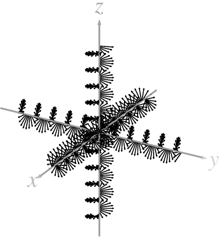
Figure 1: Cartan’s spiral staircase. Cartan’s rules cartan22 for the introduction of a non-Euclidean connection in a 3D Euclidean space are as follows: (i) A vector which is parallelly transported along itself does not change (cf. a vector directed and transported in $x$-direction). (ii) A vector that is orthogonal to the direction of transport rotates with a prescribed constant ‘velocity” (cf. a vector in $y$–direction transported in $x$–direction). The winding sense around the three coordinate axes is always positive.

Obviously, Cartan’s prescriptions are reflected in the solution (37). For (37), autoparallels and extremals coincide. Thus, in the spiral staircase, extremals are Euclidean straight lines. This is apparent in Cartan’s construction.

Cartan apparently had in mind a 3D space with Euclidean signature. For an alternative interpretation of Cartan’s spiral staircase we consider the 3D Einstein–Cartan field equations without cosmological constant:

$$\frac{1}{2}\,\eta_{\alpha\beta\gamma}\,R^{\beta\gamma} = \ell\,\Sigma_{\alpha}\,,$$ (39)

$$\frac{1}{2}\,\eta_{\alpha\beta\gamma}\,T^{\gamma} = \ell\,\tau_{\alpha\beta}\,.$$ (40)

The coframe and the connection of (37), Euclidean signature assumed, form a solution of the Einstein–Cartan field equations with matter provided the energy–momentum current (for Euclidean signature the force stress tensor ${\mathfrak{t}}_{\alpha}{}^{\beta}$) and the spin current (here the torque or moment stress tensor ${\mathfrak{s}}_{\alpha\beta}{}^{\gamma}$) are constant,

$$\Sigma_{\alpha}=:{\mathfrak{t}}_{\alpha}{}^{\beta}\,\eta_{\beta}=-\frac{{\cal T}^{2}}{\ell^{3}}\,\eta_{\alpha}\,\quad{\rm and}\quad\tau_{\alpha\beta}=:{\mathfrak{s}}_{\alpha\beta}{}^{\gamma}\,\eta_{\gamma}=-\frac{\cal T}{\ell^{2}}\,\vartheta_{\alpha\beta}\,.$$ (41)

Inversion yields

$${\mathfrak{t}}_{\alpha}{}^{\beta}=-\frac{{\cal T}^{2}}{\ell^{3}}\,\delta_{\alpha}^{\beta}\,,\qquad{\mathfrak{s}}_{\alpha\beta\gamma}=-\frac{\cal T}{\ell^{2}}\,\eta_{\alpha\beta\gamma}\,.$$ (42)

We find a constant hydrostatic pressure $-{\cal T}^{2}/\ell^{3}$ and a constant torque $-{\cal T}/\ell^{2}$, exactly as foreseen by Cartan. In solid state physics, this corresponds to a superposition of three “forests” of screw dislocations that are parallel to the coordinate axes with constant and equal densities. However, in a real crystal, the Riemann–Cartan curvature $R^{\alpha\beta}$ has to vanish (instead of the Riemannian curvature $\widetilde{R}^{\alpha\beta}$, as in our exact solution) and no pressure would emerge macroscopically.

Thus we can either view the spiral staircase as a vacuum solution and special case of our solution of Table 1 or as a material solution of 3D Einstein–Cartan theory (with Euclidean signature) carrying constant pressure and constant torque.

- (1) S. Deser, R. Jackiw, and G. ’t Hooft: Three–dimensional Einstein gravity: dynamics of flat space. Ann. Phys. (NY) 152 (1984) 220–235.
- (2) S. Carlip: Quantum Gravity in Dimensions. Cambridge University Press, Cambridge (1998).
- (3) S. Deser, R. Jackiw, S. Templeton: Topologically massive gauge theories. Ann. Phys. (NY) 140 (1982) 372–411.
- (4) A. Achúcarro and P.K. Townsend: A Chern–Simons action for three–dimensional anti–de Sitter supergravity theories. Phys. Lett. B180 (1986) 89-92.
- (5) E. Witten: dimensional gravity as an exactly soluble system. Nucl. Phys. B311 (1988/89) 46–77.
- (6) E. Witten: Topology-changing amplitudes in dimensional gravity. Nucl. Phys. B323 (1989) 113–140.
- (7) J.H. Horne and E. Witten: Conformal gravity in three dimensions as a gauge theory. Phys. Rev. Lett. 62 (1989) 501–504.
- (8) K. Koehler, F. Mansouri, C. Vaz, and L. Witten: Wilson loop observables in dimensional Chern–Simons supergravity. Nucl. Phys. B341 (1990) 167–186.
- (9) T. Dereli, Y. N. Obukhov: General analysis of self–dual solutions for the Einstein–Maxwell–Chern–Simons theory in dimensions. Phys. Rev. D62 (2000) 024013 (3 pages).
- (10) T. Dereli, Ö. Sarıoğlu: Supersymmetric solutions to topologically massive gravity and black holes in three dimensions. Phys. Rev. D64 (2001) 027501 (4 pages).
- (11) M. Blagojević: Gravitation and Gauge Symmetries. Institute of Physics Publishing, Bristol, UK (2002) pp. 479 et seq.
- (12) E. W. Mielke, P. Baekler: Topological gauge model of gravity with torsion. Phys. Lett. A156 (1991) 399–403.
- (13) P. Baekler, E.W. Mielke and F.W. Hehl: Dynamical symmetries in topological 3D gravity with torsion. Nuovo Cimento B107 (1992) 91-110.
- (14) R. Tresguerres: An exact solution of (2+1)-dimensional topological gravity in metric-affine spacetime. Phys. Lett. A168 (1992) 174–178.
- (15) T. Kawai: Poincaré gauge theory of (2+1)-dimensional gravity. Phys. Rev. 49 (1994) 2862–2871.
- (16) E. Kröner: Continuum theory of defects. In: Physics of defects, R. Balian, M. Kléman, and J.-P. Poirier (Eds.), Les Houches, École d’Été de Physique Théoretique 1980. North Holland, Amsterdam (1981).
- (17) H. Kleinert: Gauge Fields in Condensed Matter. Vol. I: Superflow and Vortex Lines. Vol. II: Stresses and Defects. World Scientific, Singapore (1989).
- (18) T. Dereli, A. Verçin: A gauge model of amorphous solids containing defects. Phil. Mag. B56 (1987) 625-631.
- (19) T. Dereli, A. Verçin: A gauge model of amorphous solids containing defects II. Chern-Simons free energy. Phil. Mag. B64 (1991) 509-513.
- (20) M.O. Katanaev, I.V. Volovich: Theory of defects in solids and three–dimensional gravity. Ann. Phys. (NY) 216 (1992) 1–28.
- (21) C. Kohler: Line defects in solid continua and point particles in –dimensional gravity. Class. Quant. Grav. 12 (1995) 2977–2993.
- (22) M. Lazar: Dislocation theory as a 3–dimensional translation gauge theory. Ann. Phys. (Leipzig) 9 (2000) 461–473
- (23) M. Lazar: An elastoplastic theory of dislocations as a physical field theory with torsion. J. Phys. A35 (2002) 1983–2004.
- (24) M. Lazar: A nonsingular solution of the edge dislocation in the gauge theory of dislocations. J. Phys. A36 (2003) 1415-1437.
- (25) M. Bañados, C. Teitelboim, J. Zanelli: Black hole in three–dimensional spacetime. Phys. Rev. Lett. 69 (1992) 1849–1851.
- (26) D. Brill: Black Holes and Wormholes in 2+1 Dimensions. Eprint Archive gr-qc /9904083.
- (27) M. Bañados, M. Henneaux, C. Teitelboim, J. Zanelli: Geometry of the black hole. Phys. Rev. D48 (1993) 1506–1525.
- (28) S. Carlip: Lectures on –dimensional gravity. J. Korean. Phys. Soc. 28 (1995) S447–S467. Eprint Archive gr-qc/9503024.
- (29) S. Carlip: The –dimensional black hole. Class. Quantum Grav. 12 (1995) 2853–2879.
- (30) M. Bañados: Notes on black holes and three dimensional gravity. AIP Conf. Proc. 490 (1999) 198–216. Eprint Archive hep-th/9903244.
- (31) D. Birmingham, I. Sachs, S. Sen: Exact results for the BTZ black hole. Int. Jour. Mod. Phys. D10 (2001) 833-857.
- (32) M. Cataldo, S. del Campo, A. García: BTZ Black Hole from gravity. Gen. Rel. Grav. 33 (2001) 1245–1255.
- (33) A. Strominger: Black hole entropy from near–horizon microstates. J. High Energy Phys. 02 (1998) 009 (11 pages).
- (34) S. Hemming, E. Keski-Vakkuri: The spectrum of strings on BTZ black holes and spectral flow in the SL(2,R) WZW model. Nucl. Phys. B 626 (2002) 363–376.
- (35) C.-M. Chen, J.M. Nester, R.-S. Tung: Quasilocal energy momentum for gravity theories. Phys. Lett. A203 (1995) 5–11. Eprint Archive gr-qc/9411048.
- (36) C.-M. Chen, J.M. Nester: Quasilocal quantities for GR and other gravity theories. Class. Quant. Grav. 16 (1999) 1279-1304. Eprint Archive gr-qc/9809020.
- (37) C.-M. Chen, J.M. Nester: A symplectic hamiltonian derivation of quasilocal energy-momentum for GR. Gravitation & Cosmology 6 (2000) 257–270. Eprint Archive gr-qc/0001088.
- (38) J.M. Nester, C.-M. Chen, Y.-H. Wu: Gravitational energy–momentum in MAG. Eprint Archive gr-qc/0011101.
- (39) Y.-H. Wu: Quasilocal energy-momentum in Metric Affine Gravity. Master thesis. National Central University, Chung-Li, Taiwan, ROC (June 2001) 66 pages.
- (40) Y.-H. Wu, C.-M. Chen, J.M. Nester: Quasilocal energy-momentum in metric-affine gravity. To be published.
- (41) F.W. Hehl, J.D. McCrea, E.W. Mielke, Y. Ne’eman: Metric-affine gauge theory of gravity: field equations, Noether identities, world spinors, and breaking of dilation invariance. Phys. Repts. 258 (1995) 1–171.
- (42) F. W. Hehl, W. Kopczyński, J. D. McCrea, W. W. Mielke: Chern-Simons terms in metric–affine space–time: Bianchi identities as Euler–Lagrange equations. J. Math. Phys. 32 (1991) 2169–2179.
- (43) M. Blagojević, M. Vasilić: Asymptotic symmetries in 3d gravity with torsion. Eprint Archive gr-ac/0301051.
- (44) A.A. Sousa, J.W. Maluf: Black holes in teleparallel theories of gravity. Eprint Archive gr-qc/0301079.
- (45) R.M. Wald: General Relativity. University of Chicago Press, Chicago (1984).
- (46) A. A. García, F. W. Hehl, C. Heinicke, A. Macías: The Cotton tensor in Riemannian spacetimes. To be published.
- (47) M.-I. Park: Statistical entropy of three-dimensional Kerr-de Sitter space. Phys. Lett. B440 (1998) 275–282.
- (48) J. Fjelstad, S. Hwang: Sectors of solutions in three–dimensional gravity and black holes. Nucl. Phys. B628 (2002) 331–360.
- (49) É. Cartan: On a generalzation of the notion of Riemann curvature and spaces with torsion. Translation from the French by G.D. Kerlick. In: Cosmology and Gravitation, P.G. Bergmann, V. De Sabbata, eds. Plenum Press, New York (1980) Pp. 489-491; see also the remarks of A. Trautman, ibid. pp. 493-496.