Coupling of Linearized Gravity to Nonrelativistic Test Particles: Dynamics in the General Laboratory Frame

Abstract

The coupling of gravity to matter is explored in the linearized gravity limit. The usual derivation of gravity-matter couplings within the quantum-field-theoretic framework is reviewed. A number of inconsistencies between this derivation of the couplings, and the known results of tidal effects on test particles according to classical general relativity are pointed out. As a step towards resolving these inconsistencies, a General Laboratory Frame fixed on the worldline of an observer is constructed. In this frame, the dynamics of nonrelativistic test particles in the linearized gravity limit is studied, and their Hamiltonian dynamics is derived. It is shown that for stationary metrics this Hamiltonian reduces to the usual Hamiltonian for nonrelativistic particles undergoing geodesic motion. For nonstationary metrics with long-wavelength gravitational waves (GWs) present, it reduces to the Hamiltonian for a nonrelativistic particle undergoing geodesic deviation motion. Arbitrary-wavelength GWs couple to the test particle through a vector-potential-like field $N_{a}$, the net result of the tidal forces that the GW induces in the system, namely, a local velocity field on the system induced by tidal effects as seen by an observer in the general laboratory frame. Effective electric and magnetic fields, which are related to the electric and magnetic parts of the Weyl tensor, are constructed from $N_{a}$ that obey equations of the same form as Maxwell’s equations . A gedankin gravitational Aharonov-Bohm-type experiment using $N_{a}$ to measure the interference of quantum test particles is presented.

I Introduction

At first glance, it would seem that the Hamiltonian dynamics of nonrelativistic, classical test particles in the linearized gravity limit has been thoroughly studied, and is well understood. Indeed, in this limit gravitational waves (GWs) are often treated as simply a spin-2 gauge field propagating in flat Minkowski spacetime Feynman (1963), and the coupling of GWs to matter would seem to follow naturally. This determination would be premature; we show in this paper that such an approach obfuscates the underlying physics of the system, and overlooks the surprising links between gravitational waves, vector potentials, and gauge symmetries.

Much of our current understanding of the coupling of matter to gravity comes from attempts at constructing quantum gravity (QG) Feynman (1963); DeWitt (1967, 1967, 1967), and from the theory of quantum fields in curved spacetime (QFCS) Birrell and Davies (1982); Wald (1994). Once the Lagrangians for various elementary particles—both gauge and nongauge—were determined in flat Minkowski spacetime, their extension to curved spacetimes was a natural next step. To make this extension of the flat spacetime Lagrangians to curved spacetimes, a number of seemingly natural assumptions were typically made then, and are still being made now. The expectation is that the experience and intuition gained from constructing quantum field theories (QFTs) in flat spacetime will serve as useful guides in constructing QFTs in curved spacetimes. Thus, flat spacetime Lagrangians for bosonic fields are promoted to curved spacetimes by replacing the Minkowski metric with the metric for a curved spacetime, the partial derivative with the covariant derivative, and the Lorentz-invariant integration measure with the general-coordinate-transformation-invariant integration measure. The extension of fermionic fields, such as spin-1/2 and -3/2 fermions, follow in much the same way once a tetrad frame is chosen. The Hilbert action from classical general relativity (GR) is used for the gravity component of the theory, and the metric for the spacetime $g_{\mu\nu}$ is identified with the gravitational field’s degree of freedom. A classical background metric $g^{0}_{\mu\nu}$ for the spacetime is chosen—in Feynman (1963) it was flat Minkowski spacetime, and in DeWitt (1967, 1967, 1967) it was either an asymptotically flat spacetime or a spacetime with finite spatial extent—and the propagating component of the gravitational field is extracted from the theory by considering fluctuations $h_{\mu\nu}$ about $g^{0}_{\mu\nu}$ combined with a suitable gauge (coordinate) choice. These fluctuations—representing gravitational waves (GWs) in GR and gravitons in QG—are then expanded about $g^{0}_{\mu\nu}$ assuming that $h_{\mu\nu}=g_{\mu\nu}-g^{0}_{\mu\nu}$ are small compared to $g^{0}_{\mu\nu}$, and are subsequently treated as simply another spin-2 non-Abelian gauge field propagating in the background spacetime. By also expanding the metric terms about $g^{0}_{\mu\nu}$ in the Lagrangians for the matter fields, one obtains terms that couple GWs—or gravitons in QG—with matter. These interaction terms would then seem to be fixed by the field’s corresponding flat spacetime Lagrangians combined with the standard prescription for promoting them to curved spacetimes.

As natural, and as straightforward, as the above prescription is for determining the coupling of matter to gravity, it nevertheless makes a number of implicit assumptions. When one tries to reconcile these assumptions with classical GR, a number of troubling inconsistencies become immediately apparent.

The first implicit assumption is that the measuring apparatus does not play a role in the theory. That is, when calculating the various effects caused by the interaction of gravity with matter—such as, say, the scattering cross section of GWs—one does not have to explicitly include the measuring apparatus. This assumption is certainly true for all the other forces of nature; the existence of opposite or canceling “charges” for the EM, weak, and strong forces ensures that one can, in principle, screen out these forces, thereby making the measuring apparatus unaffected by them. This is not true for gravity, however; one cannot screen out the gravitational force. Why, then, should one not include the measuring apparatus explicitly in the construction of QG or of QFCS? Indeed, we shall show here that one must include the effects of gravitation on the apparatus in order to obtain physically correct results.

One may argue that the scattering processes considered in quantum gravity occurs at very short length scales—the Planck length—and the presence of any measuring apparatus will have a negligibly small effect. However, we would expect from the correspondence principle that classical gravity results could be obtained—in some limit—from the quantum theory; indeed, the construction of QG Feynman (1963); DeWitt (1967, 1967, 1967) makes explicit use of the classical theory. And in classical GR it is well known that the inclusion of the measuring apparatus—along with the observer—is crucial to understanding the dynamics of certain time-varying general relativistic systems involving tidal forces.

Consider, for example, an isolated observer and a classical test particle initially at rest some distance away from him. While both the observer and the particle do not move spatially with respect to one another, they are both physical objects that move along their respective geodesics. If a GW now passes through the system, tidal forces will of course shift the position and the velocity of the particle. However, these same tidal forces will also shift the position and the velocity of the observer; the observer cannot be isolated from the effective tidal forces caused by the GW. Thus, the observer cannot measure the motion of the particle independently of his own motion; he can only measure the relative motion of the particle with respect to himself. For GWs in the long-wavelength limit, the particle appears to the observer to undergo geodesic deviation motion [Eq. (35.12) of Misner et al. (1973)], and not geodesic motion as one might first expect. Indeed, a simple derivation of the geodesic deviation equation in this limit is to take the geodesic equation for the observer, subtract from it the geodesic equation of the particle, and expand the result in the distance separating the two geodesics.

Based on this simple example we would expect that any physically measurable response of matter to the scattering of GWs calculated by using either QG or QFCS should include the effect of the GW on the observer. By extension, we would expect that in order to be consistent with classical GR, the construction of QG or QFCS should explicitly include the observer and his measurement apparatus from the very beginning.

It may also be argued that, as with the other forces, explicit inclusion of an observer would be formally correct, but not required; the lack of its inclusion would not materially affect any calculation. This argument would also be in conflict with general relativity, however.

Consider once again the simple system described above. When the geodesic deviation equations of motion are solved, one finds that the observed tidal response of the test particle to the passage of the long-wavelength GW is proportional to the distance separating the observer from the test particle; as long as the long-wavelength approximation holds, the further away the particle is from the observer, the larger its response to the GW. This ubiquitous response of classical matter to the passage of a GW is exploited in various GW detectors such as the Weber bar and LIGO (Laser Interferometry Gravitational-wave Observatory); the larger the detector, the larger its response to the passage of a GW. The characteristic size $L$ of the detector does play a role in the response of the system to the GW.

Suppose that either QG or QFCS is used to calculate the response of a Weber bar or LIGO to passage of a GW through the system. It would be natural to use the complex scalar field $\Psi$ to describe the system. Using the standard approach outlined above, it is straightforward to see that to lowest order, the coupling between a GW propagating in Minkowski spacetime with $\Psi$ is $\sim h_{\mu\nu}\partial^{\mu}\Psi^{\dagger}\partial^{\nu}\Psi$. Even in the long-wavelength limit, this interaction term does not explicitly depend on the size of the system. Moreover, it is difficult to see how such size dependence can be generated by this term.

The second implicit assumption made in Feynman (1963) and DeWitt (1967, 1967, 1967) is that one can always find a global time axis—and thereby construct a global coordinate system—in the curved spacetime. This is certainly possible for flat Minkowski spacetime, which is often used as the background spacetime. It is also possible for the asymptotically flat manifold that DeWitt considers in DeWitt (1967). However, we know from classical GR that it is not possible to find a coordinate system with a global time axis in general.

The Minkowski spacetime and the asymptotically flat spacetimes—along with the various black hole spacetimes—are stationary spacetimes. In these spacetimes one can always choose a frame where the metric does not depend explicitly on the time coordinate. Consequently, one can always construct a global timelike Killing vector, which can be used by all observers in the spacetime as their time axis (except, perhaps, at the event horizon or at an essential singularity). This Killing vector can then be used to construct what DeWitt termed the “preferred frame”, or as Hawking and Ellis termed it, a “special frame” Hawking and Ellis (1973) that all observers in that spacetime can agree to use.

Timelike Killing vectors—and global frames—do not exist in general, however. Importantly, they do not exist in the presence of a GW. Instead, each observer must choose his own local proper time axis, and construct his own local proper coordinate system from it. Consequently, one can only measure the relative motion between observers. This is the underlying physical reason why, in the example given above, one ends up with the geodesic deviation equation of motion Misner et al. (1973) in the long-wavelength limit for GWs, instead of the geodesic equation of motion.

Although the above point is made very elegantly in the beginning of Chap. 4 of Hawking and Ellis (1973) for classical GR, it is relevant on the quantum level as well. As pointed out in both Chap. 3 of Birrell and Davies (1982) and Chap. 3 of Wald (1994), the construction of Fock spaces for quantum fields in a curved spacetime is frame dependent; different choices of coordinates result in unitarily inequivalent Hilbert spaces. Thus, only for such spacetimes as the stationary and De Sitter spacetimes (considered also by DeWitt in DeWitt (1967)), where there is a “preferred frame”, will it be possible for all observers to agree on what constitutes a particle state. It does not exist in general (see Wald (1994) for a discussion of the relevance of the concept of “particles” in general spacetimes).

As dissimilar as the two above implicit assumptions may be appear to be on the surface, they are nonetheless intimately connected. The experimental measurement of any physical quantity requires an operational choice of origin, and a local orthogonal (tetrad) coordinate system. As any measurement is done through a physical apparatus, this mathematical choice of coordinate systems is fixed on a real physical object. The inclusion of the observer in the theory is thus equivalent to a choice of local coordinates; a choice of local coordinates must be equivalent to the inclusion of the physical observer.

Although we have pointed out in the above a number of inconsistencies between results from classical GR on the one hand, and QG and QFCS on the other, the goal of this paper is not to present a reformulation of either QG or QFCS; we leave that task to future research. We instead address the issues raised by the two assumptions in the above by focusing on the dynamics of a much simpler system: the nonrelativistic, classical test particle in weak gravity. As simple as this system may be, especially when compared to the counterexamples we have listed above, many of the issues that we have raised above appear here as well. Fundamentally, what is at issue here is the appropriate choice of coordinates; this is an inherent aspect of classical GR, and is not due to a subtlety in the quantum theory.

An analysis based on the dynamics of classical test particles has the added advantage of having limiting cases that have either been experimentally verified, or are in the process of being verified. In one limit, the Eötvös experiment, the advancement of the perihelion of Mercury, the deflection of light by the Sun, and the gravitational redshift are all calculable within the usual dynamics of test particles in stationary spacetimes based on the geodesic equation. In the other limit, the response of Weber bars and LIGO to the passage of GWs is calculable within the dynamics of test particles based on the geodesic deviation equation Misner et al. (1973). The result of the analysis in this paper must agree with these two limits; this serves as a stringent test of the validity of the approach we have taken and the coordinate system we have constructed.

In the literature most analyses of the dynamics of test particles in curved spacetime are done in the same vein as the construction of QG and QFT in curved spacetimes, and are a direct generalization of the usual techniques for deriving Hamiltonians from Lagrangians for particles in flat spacetimes. One starts with the usual geodesic action for the test particle moving in an arbitrary curved spacetime with a given metric $g_{\mu\nu}$. Time reparametization invariance of the action is broken either by choosing an explicit time coordinate, or by introducing a mass-shell constraint (by hand or through a Lagrange multiplier). Choosing $x^{\mu}$ as the general coordinate, the canonical momentum $p_{\mu}$ is calculated from the Lagrangian. The Hamiltonian $H_{SF}$ ($SF$ for “standard formalism”) is then constructed from this $p_{\mu}$ and the Lagrangian in the usual way. An analysis similar to this was followed by DeWitt in his 1957 paper DeWitt (1957), albeit in much more detail, and in 1966 he applied the nonrelativistic limit of $H_{SF}$ for charged test particles to the analysis of the behavior of superconductors in the Earth’s Lense-Thirring field DeWitt (1966).

It would seem that all we would have to do is to take the nonrelativistic limit of $H_{SF}$. However, the form of $H_{SF}$ is dramatically different from the Hamiltonian for test particle motion derived in Speliotopoulos (1995) based on the geodesic deviation equations of motion. As with the case of QG and QFCS the same troubling questions come to the fore at this point: Where is the observer? What are physical quantities such as the position $\vec{x}$ and velocity $\vec{v}$ of the particle measured with respect to? What frame has been implicitly chosen by this analysis? Is this frame physical? We know from the observer–test-particle example given above that these are not fatuous questions. Rather, they directly address the underlying physics.

It is certainly true that in some specific cases—such as the presence of a weak GW in the system—one can treat the time-varying part of the metric as a perturbation of one of the known stationary metrics; this time-varying piece would then be reflected as a perturbation on the Killing vector. One could then use the usual coordinate system for these spacetimes—augmented by the inclusion of the observer and his coordinate system—and calculate $H_{SF}$ in the usual way. Doing so will not elucidate the underlying physics, however, and it is difficult to see how the geodesic deviation equations of motion arises in this approach.

The approach we shall take instead in studying the dynamics of nonrelativistic test particles in the linearized gravity limit will be to construct a general coordinate system that builds in the essential physics from the very beginning. Since relative measurements between the observer and the particle always make physical sense, they are used as the foundation of our construction; the special case of stationary metrics will naturally be included. Specifically, we follow the considerations of Synge (1960) and de Felice and Clarke (1990) (see also Thorne in connection with the coordinate system used in the analysis of LIGO): Every physical particle travels along a worldline $\mathit{\Gamma}_{c}(\tau)$ with tangent vector $c^{\mu}$ (which does not need to be a geodesic) in the spacetime manifold $\mathbb{M}$. Every measurement of the physical properties of the test particle by an observer must be done using an experimental apparatus. The observer—along with his apparatus—must propagate along his own worldline $\mathit{\Gamma}_{u}(\tau)$ with tangent vector $u^{\mu}$. Consequently, every physical measurement of the particle is done relative to the motion of an observer. In particular, in measuring the position of the particle, one measures the distance separating $\mathit{\Gamma}_{c}(\tau)$ and $\mathit{\Gamma}_{u}(\tau)$; in measuring the $4$-velocity of the particle one measures of the relative velocity of the particle with respect to the observer Misner et al. (1973).

Implementation of the above considerations proceeds quite naturally. As the observer prepares to take measurements on the test particle, he first chooses a local orthonormal coordinate system. In curved spacetimes, this involves the construction of a local tetrad frame Synge (1960). Naturally, this coordinate system will be fixed, say, to the center of mass of his experimental apparatus, and will thus propagate in time along the worldline $\mathit{\Gamma}_{u}(\tau)$ as well. The observer uses the coordinate time of the physical apparatus to measure time, which, because he will not be moving relative to the apparatus, is also his proper time. Thus the time axis of the coordinate system he has chosen will always lie tangentially to $\mathit{\Gamma}_{u}(\tau)$. The position—which can be of finite extent—of the test particle is measured with respect to an origin fixed on the apparatus, and is the shortest distance between this origin and the particle. However, because the apparatus travels along its worldline, the origin of the coordinate system will also travel along a worldline in $\mathbb{M}$. Later, when the rate of change of the position of the particle is measured at two successive times, the relative $4$-velocity of the particle with respect to the apparatus will naturally be obtained. Thus, the observer constructs his usual laboratory frame that extends across his experimental apparatus, but now incorporating the nontrivial local curvature of $\mathbb{M}$. We call this frame the general laboratory frame (GLF).

Local coordinate systems fixed to an observer have been constructed before. The Fermi normal coordinates (FNC) were constructed in the 1920’s by Fermi Fermi (1922), and the Fermi Walker coordinates (FWC) were constructed in Synge (1960). While an observer can use either set of coordinates, both make assumptions and approximations that drastically limit their usefulness. The FNC—a direct implementation of the equivalence principle—are constructed so that the Levi-Civita connection $\Gamma^{\alpha}_{\mu\nu}$ vanishes identically along the worldline of the observer; only when one moves off the worldline does the curvature dependent terms begin to appear Manasse and Misner (1963). For the FWC, the restrictions on $\Gamma^{\alpha}_{\mu\nu}$ are somewhat relaxed, but certain components of $\Gamma^{\alpha}_{\mu\nu}$—such as $\Gamma^{\hat{a}}_{\hat{0}\hat{b}}$ where $\hat{a}$, $\hat{b}$ are spatial indices—still vanish along the worldline. Once again, when one moves off the worldline curvature terms appear in the form of the Riemann tensor and its derivatives. In both, one effectively makes a derivative expansion in the Riemann curvature tensor Mashhoon (1975, 1977); Li and Wi (1979); Nesterov (1999).

In both FNC and FWC systems, choices for the value of $\Gamma^{\alpha}_{\mu\nu}$—a gauge choice—have been made, and in both systems such gauge choices are inconsistent with the usual transverse-traceless (TT) gauge for GWs. While it is possible to study the interaction of GWs with test particles in these coordinate systems (see Fortini and Gualdi (1982); Baroni (1986); Flores and Orlandini (1986) for FNC and Chicone and Mashhoon (2002) for FWC), doing so is cumbersome. For example, it has only recently been established that the TT gauge for GWs is compatible with the FNC Faraoni (1992), but only in the long wavelength limit; the two are incompatible when the wavelength becomes smaller than the size of the experimental apparatus. In our construction of the GLF, no such restrictions on $\Gamma^{\alpha}_{\mu\nu}$ are made within the linearized gravity approximation. Thus, when we consider the case of GWs interacting with nonrelativistic particles, the TT gauge—or any other gauge—can be directly taken. Moreover, we do not make any restrictions on how rapidly the Riemann curvature tensor varies, and therefore are not restricted to only the long-wavelength limit. This enables us to study the effects of arbitrary-wavelength GWs on the motion of nonrelativistic test particles in large systems.

It is here in our study of test particle dynamics that we obtain our most surprising result: Even though the underlying GW is a spin-$2$ tensor field, in the weak gravity, slow velocity limit, the GW acts on the particle through a local velocity field $N_{a}$. This velocity field—which is an integral of the Ricci rotation coefficients—couples to the test particle as though it was a vector potential for a spin-$1$ vector field (see also Chiao (2003) for the additional terms that the Ricci rotation coefficients introduce in fermionic condensed matter systems and their implications), and its origin is the tidal nature of the forces that the GW induces on the test particle. It has the same properties as a vector potential: Like the vector potential for the EM field $A_{a}$, $N_{a}$ is a transverse field satisfying the wave equation. It is a frame-dependent field with the local Galilean group as its gauge group. Effective “electric” and “magnetic” fields can be constructed from $N_{a}$ in the usual way, and they are solutions to a set of partial differential equations that have the same form as the Maxwell equations since they are directly related to the electric and magnetic parts of the Weyl tensor, and thus to components of the Riemann curvature tensor. The equations of motion for the nonrelativistic particle have the form of a Lorentz force with the mass of the particle playing the role of the charge. As required, these equations reduce to the usual geodesic deviation equations Misner et al. (1973) in the long-wavelength limit.

The rest of this paper is organized as follows. In Sec. II we construct explicitly the GLF and its coordinates using a tetrad frame fixed to the worldline of the observer. The velocity of a test particle in the GLF is derived in the nonrelativistic limit. In Sec. III we use these velocities to construct the action, and then the Hamiltonian for the test particle in the GLF. We show that for stationary $\mathbb{M}$ this Hamiltonian reduces to DeWitt’s Hamiltonian, and for long-wavelength TT GWs propagating in a flat background it reduces to the Hamiltonian Speliotopoulos (1995) derived from the geodesic equations of motion. In Sec. IV, we study the properties of the velocity field $N_{a}$ introduced in Sec. 3 for arbitrary GWs, and construct effective electric and magnetic fields from it. These fields are shown to obey equations that have the same form as Maxwell’s equations, and they are used to derive the equations of motion for a test particle. An Aharonov-Bohm-type interference effect for quantum test particles that is shown to follow from the effective vector potential $N_{a}$ can be found in Sec. V along with other concluding remarks. In Appendix A we present a brief review of the tetrad and linearized gravity formalisms, while in Appendix B, we derive the nonintegrable phase factor $\exp\{i(m/\hbar)\oint N_{A}dX^{A}\}$ for the gravitational Aharonov-Bohm-type interference effect.

II Construction of the GLF

As usual, $g_{\mu\nu}(x)$ is the metric on the curved spacetime manifold $\mathbb{M}$ with a signature $(-1,1,1,1)$. Greek indices run from $0$ to $3$, and they denote the coordinates $x^{\mu}$ for a general coordinate system on $\mathbb{M}$. We will, however, be working primarily in one specific tetrad frame, and we will use capital Roman letters running from $0$ to $3$ for the spacetime indices in this frame. (A summary of well-known results for linearized gravity and tetrad frames is given in Appendix A.) We reserve lowercase Roman letters running from $1$ to $3$ for spatial indices in the tetrad frame, and careted lowercase Roman letters for spatial indices in the general coordinate frame. A worldline with a timelike tangent vector $u^{\mu}$ parameterized by $\tau$ is denoted as $\mathit{\Gamma}_{u}(\tau)$; this worldline needs not be a geodesic. Spacelike geodesics, with tangent vectors $\chi^{\mu}$ and parameterized by its arclength $s$, are denoted by $\mathit{\gamma}_{\chi}(s)$, and null geodesics with tangent vectors $\pi^{\mu}$ parameterized by its arclength $\sigma$ are denoted by $\mathit{\gamma}_{\pi}(\sigma)$.

The construction of the GLF for the observer—being a specific choice of general tetrad frames that is fixed onto the worldline of the observer—is fairly standard. It must, however, be done without knowing the specific form of the underlying metric of $\mathbb{M}$. Indeed, the local metric at any given time is determined by making local measurements. We are aided in this construction by three observations. First and foremost, we note that the observer does not need a coordinate system that is nonsingular over all of $\mathbb{M}$; such a coordinate system is known not to exist in general. All that is needed is a coordinate system that is nonsingular within the region of $\mathbb{M}$ where the observer makes experimental measurements. Second, we are working in the linearized gravity limit. This assures that we do not have to concern ourselves with coordinate singularities, and we can take curvature effects as perturbations on the flat spacetime metric. Finally, we are primarily interested in the effect of linearized gravity on nonrelativistic test particles; in this limit, incorporation of causality effects in the construction of the GLF simplifies dramatically.

Let us consider an observer $\mathcal{O}$ with worldline $\mathit{\Gamma}_{u}(\tau)$. To perform experimental measurements at some time $\tau_{0}$, $\mathcal{O}$ constructs a local orthogonal coordinate system centered on his experimental apparatus by choosing a tetrad frame $\{{}_{o}e_{A}^{\>\>\>\>\mu}(\tau_{0})\}$, a set of orthogonal unit vectors such that $\eta_{AB}={}_{o}e_{A}^{\>\>\>\>\mu}(\tau_{0})\>\>g_{\mu\nu}|_{\mathit{\Gamma}_{u}(\tau_{0})}\>\>{}_{o}e_{B}^{\>\>\>\>\nu}(\tau_{0})$, where $\eta_{AB}$ is the usual Minkowski metric and $g_{\mu\nu}|_{\mathit{\Gamma}_{u}(\tau_{0})}={}_{o}e_{A\mu}(\tau_{0})\>\>\eta^{AB}\>\>{}_{o}e_{B\nu}(\tau_{0})$ is the metric for $\mathbb{M}$ at $\mathit{\Gamma}_{u}(\tau_{0})$. We use the presubscript $o$ (for “observer”) on ${}_{o}e_{0}^{\>\>\>\>\mu}$ to emphasize that at this point the frame only exists on $\mathit{\Gamma}_{u}(\tau)$. Unlike the general tetrad frame, we require that $u^{\mu}(\tau_{0})={}_{o}e_{0}^{\>\>\>\>\mu}(\tau_{0})$; the time axis of the frame at $\tau_{0}$ lines up with the worldline of the observer. As usual, tetrad indices are raised and lowered by $\eta_{AB}$, and general coordinate indices are raised and lowered by $g_{\mu\nu}$.

For the coordinate system at subsequent times we have to transport ${}_{o}e_{A}^{\>\>\>\>\mu}$ along $\mathit{\Gamma}_{u}(\tau)$ in such a way that that ${}_{o}e_{0}^{\>\>\>\>\mu}$ always points along $u^{\mu}$. If $\mathit{\Gamma}_{u}(\tau)$ were a geodesic, we would only need to parallel transport $e_{A}^{\>\>\>\>\mu}$ along it. However, because we are interested in nongeodesic worldlines we must instead use Fermi-Walker transport, a generalization of parallel transport that subtracts the nongeodesic motion of $\mathit{\Gamma}_{u}(\tau)$ from the transport of ${}_{o}e_{A}^{\>\>\>\>\mu}$. For any vector $v^{\mu}$ and a tangent vector $\chi^{\mu}$ to some worldline $\mathit{\Gamma}_{\chi}$, the Fermi-Walker transport of $v^{\mu}$ along $\mathit{\Gamma}_{\chi}$ is

$$\frac{D^{F}v^{\mu}}{\partial\tau}=\frac{Dv^{\mu}}{\partial\tau}-\left(v_{\nu}\frac{D\chi^{\nu}}{\partial\tau}\right)\chi^{\mu}+\left(v_{\nu}\chi^{\nu}\right)\frac{D\chi^{\mu}}{\partial\tau},$$ (1)

where as usual parallel transport along $\mathit{\Gamma}_{\chi}$ is

$$\frac{Dv^{\mu}}{\partial\tau}=\frac{\partial v^{\mu}}{\partial\tau}+\Gamma^{\mu}_{\alpha\beta}\chi^{\alpha}v^{\beta},$$ (2)

and $\Gamma^{\mu}_{\alpha\beta}$ is the connection on $\mathbb{M}$.

By the Fermi-Walker transport of ${}_{o}e_{A}^{\>\>\>\>\mu}(\tau)$ along $\mathit{\Gamma}_{u}(\tau)$, we find at each time $\tau>\tau_{0}$,

$$\frac{D^{F}{}_{o}e_{0}^{\>\>\>\>\mu}(\tau)}{\partial\tau}\equiv 0.$$ (3)

Not surprisingly ${}_{o}e_{0}^{\>\>\>\>\mu}(\tau)$ automatically undergoes Fermi-Walker transport. The spatial tetrads, on the other hand, do not, and are solutions of the linear partial differential equations

$$0=\frac{D{}_{o}e_{a}^{\>\>\>\>\mu}(\tau)}{\partial\tau}-\left({}_{o}e_{a}^{\>\>\>\>\nu}(\tau)\frac{D{}_{o}e_{0\nu}(\tau)}{\partial\tau}\right){}_{o}e_{0}^{\>\>\>\>\mu}(\tau),$$ (4)

with the appropriate initial condition at $\tau=\tau_{0}$.

To extend $\{{}_{o}e_{A}^{\>\>\>\>\mu}(\tau)\}$ off $\mathit{\Gamma}_{u}(\tau)$ we once again use the Fermi-Walker transport of $e_{A}^{\>\>\>\>\mu}$, but now in directions perpendicular to $\mathit{\Gamma}_{u}(\tau)$. At any fixed time $\tau$, let $\mathit{\gamma}_{\chi}^{\tau}(s)$ be a spacelike geodesic such that $u^{\mu}\chi_{\mu}=0$ and $\mathit{\gamma}_{\chi}^{\tau}(0)=\mathit{\Gamma}_{u}(\tau)$ (see Fig. 1).

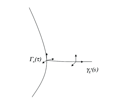
Figure 1: Parallel transport of $e_{A}^{\>\>\>\>\mu}$ off $\mathit{\Gamma}_{u}(\tau)$ and along a spacelike geodesic $\mathit{\gamma}_{\chi}^{\tau}(s)$.

We include the superscript $\tau$ on $\mathit{\gamma}_{\chi}^{\tau}(s)$ to denote the implicit dependence of $\mathit{\gamma}_{\chi}^{\tau}(s)$ on $\tau$. For geodesics, Fermi-Walker transport is equivalent to parallel transport, and $e_{A}^{\>\>\>\>\mu}(\tau,s)$ are solutions of

$$0=\frac{De_{A}^{\>\>\>\>\mu}(\tau,s)}{\partial s},$$ (5)

along $\chi^{\mu}$ with the initial condition $e_{A}^{\>\>\>\>\mu}(\tau,0)={}_{o}e_{A}^{\>\>\>\>\mu}(\tau)$ for each time $\tau$. It is straightforward to show from Eq. $(\ref{5})$ that $e_{A}^{\>\>\>\>\mu}(\tau,s)\>e_{B\mu}(\tau,s)=\eta_{AB}$. Consequently, we can now consider $e_{A}^{\mu}$ to be a vector field on $\mathbb{M}$ such that

$$g_{\mu\nu}=e^{A}_{\>\>\>\>\mu}\>e_{A\nu},\qquad\eta_{AB}=e_{A}^{\>\>\>\>\mu}\>e_{B\mu}.$$ (6)

While the above defines a set of orthonormal vectors for the observer, we still have to construct explicit coordinates for this frame. As mentioned in the Introduction, observer-based coordinates have been constructed before Fermi (1922), Synge (1960), although they were not explicitly constructed in a tetrad frame. Although the FNC and FWC are constructed using a series of approximations that make them unsuitable for our purposes, a number of the fundamental concepts used in their construction nevertheless carry over to our construction. In particular, Synge Synge (1960) introduces the notion of the world function to construct both coordinate systems (see also de Felice and Clarke (1990)). This extended object is a scalar function that measures the length squared between two points connected by a geodesic on $\mathbb{M}$ that are separated by a finite distance. It serves as a two-point correlation function that measures the net effect of the differences in local curvature between the two points. Moreover, because the world function is a length—and thus a scalar invariant—it is expandable in terms of the Riemann curvature tensor and its derivatives, thereby avoiding many coordinate-dependent artifacts.

Useful though the world function may be, with the tetrad frame constructed above we have a more direct method of constructing coordinates. (This method is similar to the approach followed in Nesterov (1999) for the FNC.) Like Synge, our method makes use of an extended object between two points on $\mathbb{M}$, and we explicitly introduce a test particle $\mathcal{P}$ with worldline $\mathit{\Gamma}_{c}(\tau)$ that is close enough to $\mathit{\Gamma}_{u}(\tau)$ for its physical properties to be measured by $\mathcal{O}$’s experimental apparatus. We ask what the coordinates of this particle are in $\mathcal{O}$’s frame. To be consistent with $\mathcal{O}$’s experimental measurements, we parameterize $\mathit{\Gamma}_{c}(\tau)$ by the proper time of $\mathcal{O}$, not $\mathcal{P}$. Then let $X^{A}(\tau)$ be the position of $\mathcal{P}$ at any time $\tau$ in the observer’s frame. $X^{A}(x):x^{\mu}\to X^{A}$ can also be considered as a coordinate transformation from the general coordinates $x^{\mu}$ to the tetrad frame at any time $\tau$, which in a small neighborhood $\mathcal{U}_{\mathcal{O}}$ of $\mathcal{O}$ is

$$\eta_{AB}\>dX^{A}dX^{B}=\frac{\partial X^{A}}{\partial x^{\mu}}\bigg{|}_{\mathcal{U}_{\mathcal{O}}}\frac{\partial X^{B}}{\partial x^{\nu}}\bigg{|}_{\mathcal{U}_{\mathcal{O}}}dx^{\mu}dx^{\mu},$$ (7)

so that from Eq. $(\ref{6})$,

$$\frac{\partial X^{A}}{\partial x^{\mu}}|_{\mathcal{U}_{\mathcal{O}}}=e^{A}_{\>\>\>\>\mu},\qquad\hbox{or}\qquad\frac{\partial x^{\mu}}{\partial X^{A}}|_{\mathcal{U}_{\mathcal{O}}}=e_{A}^{\>\>\>\>\mu}.$$ (8)

Taking the derivative of the first equation in Eq. $(\ref{8})$ with respect to $x^{\nu}$, we find that the integrability condition: $\partial_{\nu}e^{A}_{\mu}=\partial_{\mu}e^{A}_{\nu}$. This condition only holds within $\mathcal{U}_{\mathcal{O}}$ (see Eq. $(\ref{64})$). To extend $X^{A}$ off $\mathcal{O}$’s worldline, we note the following.

Solutions of Eqs. $(\ref{8})$ are clearly path dependent. For spatial components $X_{a}$, we consider again the spacelike geodesic $\mathit{\gamma}_{\chi}^{\tau}(s)$, but now connecting $\mathit{\Gamma}_{u}(\tau)$ to $\mathit{\Gamma}_{c}(\tau)$ such that $\mathit{\gamma}_{\chi}^{\tau}(0)=\mathit{\Gamma}_{u}(\tau)$ and $\mathit{\gamma}_{\chi}^{\tau}(s_{1})=\mathit{\Gamma}_{c}(\tau)$. (See Fig. 2.)

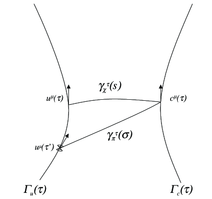
Figure 2: A sketch of the worldlines $\mathit{\Gamma}_{u}(\tau)$ and $\mathit{\Gamma}_{c}(\tau)$ of observer $\mathcal{O}$ and test particle $\mathcal{P}$, respectively, with the spacelike $\mathit{\gamma}_{\chi}^{\tau}(s)$ and null $\mathit{\gamma}_{\pi}(\sigma)$ geodesics used to construct $X^{A}$ shown. The end points of both geodesics are fixed onto specific points on $\mathit{\Gamma}_{u}(\tau)$ and $\mathit{\Gamma}_{c}(\tau)$. The simultaneity with respect to the observer $\mathcal{O}$ in time along $\mathit{\gamma}_{\chi}^{\tau}(s)$ is an approximation that only holds in the linearized gravity and nonrelativistic limits.

By integrating Eq. $(\ref{8})$ along this geodesic, we obtain the spatial coordinates of the test particle

$$X_{a}(\tau)=\int_{\mathit{\gamma}_{\chi}^{\tau}(0)}^{\mathit{\gamma}_{\chi}^{\tau}(s_{1})}e_{a\mu}(\tau,s)\chi^{\mu}(\tau,s)ds\equiv\int_{\mathit{\gamma}_{\chi}^{\tau}(s)}\bm{e}_{a},$$ (9)

as a straightforward extension of the tetrad framework to coordinates. We have made use of differential forms through $\bm{e}_{A}=e_{A\mu}\bm{d}x^{\mu}$ (see Appendix A); this will greatly simplify our analysis later. In defining Eq. $(\ref{9})$, we have explicitly assumed that the partial differential equations in Eq. $(\ref{8})$ are integrable. While this is not true for general spacetimes because of the presence of singularities, they are integrable in the weak gravity limit that we are working in. We also note that the length of $X_{a}$ is proportional to the proper length $s_{1}$ of $\gamma_{\chi}^{\tau}$.

Like the world function, $X_{a}(\tau)$ is an extended function of two points—one on the worldline of $\mathcal{O}$ and the other on the worldline of $\mathcal{P}$. Indeed, it is straightforward to see that the spatial coordinates in the FWC are an approximation of Eq. $(\ref{9})$ by taking $\chi^{\mu}$ as a constant equal to its value on $\mathit{\gamma}_{\chi}^{\tau}(0)$; the remaining integral is proportional to the world function. We emphasize, however, (the index $a$ notwithstanding) that $X_{a}$ is the integral of a differential form, and is a scalar function on $\mathbb{M}$ (see Appendix A).

The construction of the time component of the test particle $X_{0}(\tau)$ is more complicated because of causality. As Synge pointed out in his derivation of the FWC, using spacelike geodesics $\mathit{\gamma}_{\chi}^{\tau}(s)$ in Eq. $(\ref{9})$ is somewhat artificial; no physical measurements ever take place along spacelike geodesics. Strictly speaking, we should have instead used null vectors—corresponding to optical measurements—in the above. However, this would have resulted in a set of optical coordinates, and since we are primarily interested in the motion of a nonrelativistic test particle, would have been needlessly complicated. Instead, we note that in the nonrelativistic limit the forward lightcone of the observer opens up, and the observer’s null geodesic is well approximated by a spacelike geodesic in this limit; we would thus expect the above construction of $X_{a}$ to be valid in the nonrelativistic limit. The same argument cannot be made for the coordinate time $X_{0}$ of $\mathcal{P}$, however; causality still has to be taken into account. For this coordinate, we first construct $X_{0}$ using null geodesics, and then take the appropriate nonrelativistic limit.

Figure2 shows explicitly the null geodesic and spatial geodesics that we use in this construction. At a time $\tau^{\prime}<\tau$, let $\mathit{\gamma}_{\pi}(\sigma)$ be a null geodesic that connects $\mathcal{O}$ at time $\tau^{\prime}$ to $\mathcal{P}$ at time $\tau$: $\mathit{\gamma}_{\pi}(0)=\mathit{\Gamma}_{u}(\tau^{\prime})$ and $\mathit{\gamma}_{\pi}(\sigma_{1})=\mathit{\Gamma}_{c}(\tau)$. We define

$$X_{0}(\tau)=\int_{\mathit{\gamma}_{\pi}(0)}^{\mathit{\gamma}_{\pi}(\sigma_{1})}e_{0\mu}\bigg{(}\tau(\sigma),s(\sigma)\bigg{)}\pi^{\mu}(\sigma)d\sigma-\left(-\int_{\tau^{\prime}}^{\tau}e_{0\mu}(\tilde{\tau},0)u^{\mu}(\tilde{\tau})d\tilde{\tau}\right).$$ (10)

The first term in Eq. $(\ref{10})$ is the time it takes an optical signal to reach $\mathcal{P}$. The second term is the amount of time that passes for the observer for the optical signal to reach $\mathcal{P}$. Since ${}_{o}e_{0\mu}=u^{\mu}$,

$$X_{0}(\tau)=-\left(\tau-\tau^{\prime}\right)+\int_{\mathit{\gamma}_{\pi}(\sigma)}\bm{e}_{0}.$$ (11)

Note that because $u^{\mu}\chi_{\mu}=0$, unlike $X_{a}$ we cannot simply replace $\pi^{\mu}$ by $\chi^{\mu}$ in the nonrelativistic limit; the second term in Eq. $(\ref{11})$ would vanish automatically. This limit has to be taken much more carefully .

The position of the test particle was arbitrary and could have been placed at any point near $\mathit{\Gamma}_{u}(\tau)$. Thus the GLF is a combination of a tetrad frame $\{e_{A}^{\>\>\>\>\mu}\}$ fixed to the worldline of the observer together with the coordinates $(\tau,X^{a})$. It is important to note that $X^{a}$ measures the relative separation between the worldlines of $\mathcal{O}$ and of $\mathcal{P}$. For “small” $X^{a}$ , and for $\mathit{\Gamma}_{u}(\tau)$ and $\mathit{\Gamma}_{c}(\tau)$ geodesics, $X^{a}$ is simply the geodesic deviation between $\mathcal{O}$ and $\mathcal{P}$. We have also chosen, as most physical, to use the proper time of the observer as our time coordinate; Eq. $(\ref{11})$ gives the dependence of the test particle’s coordinate time on $\tau$. As we usually use the frame where the observer is at rest in the GLF, $\tau$ coincides with the coordinate time of $\mathcal{O}$. We shall simply use $\tau$ as the time variable for $\mathcal{O}$ to avoid introducing additional notation.

In what follows, the final expressions of all physical quantities measured in the GLF will be expressed in terms of $(\tau,X^{a})$, the coordinates that $\mathcal{O}$ measures in the GLF. In the frame, $u^{A}\equiv e^{A}_{\>\>\>\>\mu}u^{\mu}=\delta^{A}_{0}$, and $u^{A}$ points along the time direction for the observer, while $\chi^{A}(\tau,s)\equiv e^{A}_{\>\>\>\>\mu}\chi^{\mu}(\tau,s)$ is a scalar function in the GLF such that

$$\frac{\partial\chi^{A}}{\partial s}=\frac{D\chi^{\mu}}{\partial s}e^{A}_{\>\>\>\>\mu}+\chi^{\mu}\frac{De^{A}_{\>\>\>\>\mu}}{\partial s}=0.$$ (12)

The first term vanishes because $\mathit{\gamma}_{\chi}^{\tau}(s)$ is a geodesic, and the second term vanishes from the construction of $e^{A}_{\>\>\>\>\mu}$ in Eq. $(\ref{5})$. Thus in the GLF $\chi^{A}=\chi^{A}(\tau)$ only. In addition, since $0=\chi_{\mu}u^{\mu}=\chi_{A}\delta^{A}_{0}$, $\chi^{0}=0$ and $\chi^{A}$ is a unit spatial vector pointing directly at the test particle at any time $\tau$ . As a final point on notation, although $\partial_{a}\equiv\partial/\partial X^{a}=e_{a}^{\>\>\>\>\mu}\partial_{\mu}$, to avoid confusion we shall always write $\partial/\partial\tau$ instead of $\partial_{0}$, which is instead reserved for $\partial/\partial X^{0}$.

We now turn our attention to finding the 4-velocity of a test particle as measured in the GLF. To do so we refer to Fig. 3, which shows the position of both the observer and the particle at two subsequent times $\tau$ and $\tau+\delta\tau$.

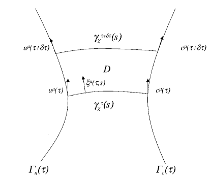
Figure 3: The location of $\mathcal{O}$ and $\mathcal{P}$ at two subsequent times, and the spacelike geodesics used in constructing $X_{a}$ as they propagate along their worldlines. The closed rectangular region $D$ used in Eq. $(\ref{14})$ is shown also. Notice that the vector $\xi^{\mu}$ as it varies along $\mathit{\gamma}_{\chi}^{\tau}(s)$.

Note that both the observer and the observed are moving: $\mathcal{O}$ along its worldline $\mathit{\Gamma}_{u}(\tau)$ and $\mathcal{P}$ along its worldline $\mathit{\Gamma}_{c}(\tau)$. The observer can only measure the relative $4$-velocity between $\mathcal{P}$ and himself. Beginning with the spatial coordinates, we take

$$\frac{dX_{a}}{d\tau} \equiv \lim_{\delta\tau\to 0}\frac{X_{a}(\tau+\delta\tau)-X_{a}(\tau)}{\delta\tau},$$ (13)

$$= \lim_{\delta\tau\to 0}\frac{1}{\delta\tau}\left\{\int_{\mathit{\gamma}_{\chi}^{\tau+\delta\tau}(s)}\bm{e}_{a}-\int_{\mathit{\gamma}_{\chi}^{\tau}(s)}\bm{e}_{a}\right\},$$

where $\mathit{\gamma}_{\chi}^{\tau+\delta\tau}(s)$ and $\mathit{\gamma}_{\chi}^{\tau}(s)$ are spacelike geodesics from $\mathcal{O}$ to $\mathcal{P}$ at $\tau+\delta\tau$ and $\tau$, respectively (see Fig. 3). Adding and subtracting integrals along the worldlines of $\mathcal{O}$ and $\mathcal{P}$,

$$\frac{dX_{a}}{d\tau} = -\lim_{\delta\tau\to 0}\frac{1}{\delta\tau}\left\{\int_{\partial D}\bm{e}_{a}+\int_{\tau}^{\tau+\delta\tau}e_{a\mu}(\tilde{\tau},0)u^{\mu}(\tilde{\tau})d\tilde{\tau}-\int_{\tau}^{\tau+\delta\tau}e_{a\mu}(\tilde{\tau},s_{1})c^{\mu}(\tilde{\tau})d\tilde{\tau}\right\},$$ (14)

$$= c_{a}(\tau,X^{a})-\lim_{\delta\tau\to 0}\frac{1}{\delta\tau}\int_{D}\bm{de}_{a},$$

where $c_{A}=e_{A\mu}(\tau,X^{a})c^{\mu}(\tau)$ is the $4$-velocity of the test particle in the GLF. $D$ is the closed region bounded by $\mathit{\gamma}_{\chi}^{\tau}(s)$, $\mathit{\gamma}_{\chi}^{\tau+\delta\tau}(s)$, and the worldlines $\mathit{\Gamma}_{u}(\tau)$ and $\mathit{\Gamma}_{c}(\tau)$ between $\tau$ and $\tau+\delta\tau$.

We parameterize the region $D$ by the $1$-forms $\bm{d}l^{\mu}_{1}=\chi^{\mu}\bm{d}s$ and $\bm{d}l^{\mu}_{2}=\xi^{\mu}\bm{d}\tau$ where

$$\xi^{\mu}\equiv\frac{D\chi^{\mu}}{\partial\tau},$$ (15)

is a function of $(\tau,s)$. Because $\chi_{\mu}\chi^{\mu}=1$, then $\xi_{\mu}\chi^{\mu}=0$, and $\bm{d}l^{\mu}_{1}$ and $\bm{d}l^{\mu}_{2}$ are linearly independent. From Eq. $(\ref{64})$, $\bm{de}_{a}=\bm{e}^{B}\wedge\bm{\omega}_{aB}$ where $\bm{\omega}_{aB}=e_{a}^{\>\>\>\>\nu}\nabla_{\mu}e_{B\nu}\bm{d}x^{\mu}$ is the Ricci coefficient 1-form. Then,

$$\int_{D}\bm{de}_{a}=-\int_{\tau}^{\tau+\delta\tau}\int_{0}^{s_{1}}\left(e^{B}_{\>\>\>\>\mu}\omega_{\nu aB}-e^{B}_{\>\>\>\>\nu}\omega_{\mu aB}\right)\xi^{\mu}\chi^{\nu}d\tilde{\tau}ds.$$ (16)

The limit $\delta\tau\to 0$ is now trivial to take, leaving only a path integral along $\bm{\gamma}_{\chi}^{\tau}(s)$. Then

$$c_{a} = \frac{dX_{a}}{d\tau}+\int_{0}^{X_{a}}\left\{\omega_{Bac}-\omega_{caB}\right\}\xi^{B}d\tilde{X}^{c},$$ (17)

$$= \frac{dX_{a}}{d\tau}+\int_{0}^{X_{a}}\left\{\langle{\xi,\bm{\omega}_{ac}}\rangle\bm{e}^{c}-\langle{\xi,\bm{e}^{B}}\rangle\bm{\omega}_{aB}\right\},$$

where we have now expressed the path integral in GLF coordinates by using $d\tilde{X}^{c}=e^{c}_{\>\>\>\>\mu}\>\chi^{\mu}d\tilde{\tau}$, and $\xi^{A}\equiv e^{A}_{\>\>\>\>\mu}\xi^{\mu}$. As usual, $\langle{\xi,\bm{\omega}_{ac}}\rangle=\xi^{\mu}\omega_{\mu ac}$.

To determine $\xi$, we note that $\xi^{\mu}$ measures the deviation in the geodesic $\mathit{\gamma}_{\chi}^{\tau+\delta\tau}(s)$ from $\mathit{\gamma}_{\chi}^{\tau}(s)$ at any time $\tau$ along $s$, and is thus the solution of the geodesic deviation (or Jacobi) equation in $s$ Synge (1960). In the GLF,

$$0=\frac{\partial^{2}\xi^{A}}{\partial s^{2}}+\tilde{R}^{A}_{\>\>\>\>B}\xi^{B}$$ (18)

where $\xi^{A}\equiv e^{A}_{\>\>\>\>\mu}\xi^{\mu}$ and $\tilde{R}^{A}_{\>\>\>\>B}\equiv R^{A}_{\>\>\>\>CBD}\chi^{C}\chi^{D}$ (see Appendix A). Note that $\chi^{A}$ is independent of $s$ and only fixes a direction in the above.

From Fig. 3 we see that $\xi^{A}$ interpolates between the tangent vector to the worldline of $\mathcal{O}$, and the tangent vector to the worldline of $\mathcal{P}$. Since $\xi^{A}\chi_{A}=\xi^{\mu}\chi_{\mu}=0$, the precise boundary conditions are: $\lim_{s\to 0^{+}}\xi^{A}(\tau,s)=\delta^{A}_{0}$ and $\lim_{s\to s_{1}^{-}}\xi^{A}(\tau,s)=\left(\delta^{A}_{B}-\chi^{A}\chi_{B}\right)c^{B}$. However, $\xi^{A}$ appears in Eq. $(\ref{16})$ through of the 2-form $\bm{d}l^{\mu}_{1}\wedge\bm{d}l^{\nu}_{2}$. Since $\bm{d}l^{\mu}_{2}$ lies parallel to $\chi^{\mu}$, this automatically projects to zero any component of $\xi^{A}$ parallel to $\chi^{A}$. Consequently, we can without loss of generality replace the second boundary condition by the much simpler condition $\lim_{s\to s_{1}^{-}}\xi^{A}(\tau,s)=c^{A}$. Equation $(\ref{18})$ can then be solved iteratively, and

$$\xi^{A}(\tau,s)=\frac{1}{s_{1}}\left\{s\>c^{A}(\tau)+(s_{1}-s)\delta^{A}_{0}\right\}+\int_{0}^{s_{1}}\tilde{R}^{A}_{\>\>\>\>B}(\tau,s^{\prime})\xi^{B}(\tau,s^{\prime})G(s,s^{\prime})ds^{\prime},$$ (19)

where $G(s,s^{\prime})$ is the Green’s function

$$G(s,s^{\prime})=\frac{s}{s_{1}}(s_{1}-s^{\prime})\theta(s^{\prime}-s)+\frac{s^{\prime}}{s_{1}}(s_{1}-s)\theta(s-s^{\prime}),$$ (20)

and $\theta(x)$ is the Heaviside function.

For $c_{0}$ we proceed the same way. Using now the diagram in Fig. 4,

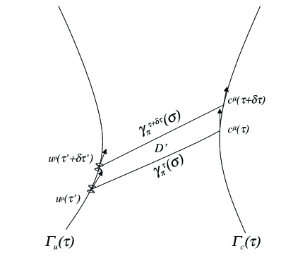
Figure 4: The null geodesics used in constructing $X_{0}$ at two subsequent times as $\mathcal{O}$ and $\mathcal{P}$ propagate along their worldlines. The closed region $D^{\prime}$ used in Eq. $(\ref{21})$ is shown.

$$c_{0}=\frac{dX_{0}}{d\tau}+\lim_{\delta\tau\to 0}\frac{1}{\delta\tau}\int_{D^{\prime}}\bm{e}^{a}\wedge\bm{\omega}_{0a}.$$ (21)

To parameterize $D^{\prime}$, we again take $\bm{d}l^{\mu}_{1}=\pi^{\mu}\bm{d}\sigma$, but now $\bm{d}l^{\mu}_{2}=\zeta^{\mu}\bm{d}\tau$ where, in the GLF,

$$\zeta^{A}(\tau,\sigma)=\delta^{A}_{0}+\left\{c^{A}(\tau)-\delta^{A}_{0}\right\}\frac{\sigma}{\sigma_{1}}.$$ (22)

Clearly, $\zeta^{A}$ and $\pi^{A}$ are linearly independent. Unlike the spatial components of the 4-velocity, we cannot use $e^{A}_{\>\>\>\>\mu}D\pi^{\mu}/\partial\tau$ to parameterize $D^{\prime}$, because it is either a null vector or a spacelike vector. Although like $\xi^{A}$, $\zeta^{A}$ interpolates between the tangent vector at $\mathit{\Gamma}_{u}(\tau^{\prime})$ and the tangent vector at $\mathit{\Gamma}_{c}(\tau)$, it does not include the corrections due to nonvanishing curvature that Eq. $(\ref{18})$ does. Because we will be working in the linearized gravity limit, such correction terms are of the order $h_{AB}$ times the particle velocity, and can be neglected to lowest order. We therefore get

$$c_{0}=\frac{dX_{0}}{d\tau}+\int_{\bm{\gamma}_{\pi}^{\tau}(\sigma)}\left\{\langle\zeta,\bm{\omega}_{0A}\rangle\bm{e}^{A}-\langle\zeta,\bm{e}^{A}\rangle\bm{\omega}_{0A}\right\}.$$ (23)

Equations $(\ref{17})$ and $(\ref{23})$ in principle determine the components of the $4$-velocity $c^{A}$ of the test particle in the GLF. However, because both $\xi^{A}$ and $\zeta^{A}$ themselves depend $c^{A}$, these equations form a set of coupled integral equations in $c^{A}$. While these equations can be solved iteratively using Eq. $(\ref{19})$ and Eq. $(\ref{22})$, we are primarily interested in the behavior of nonrelativistic test particles in the linearized gravity limit. In fact, much of our construction of the coordinates for the GLF is only valid for the nonrelativistic test particle. We thus keep only terms linear in $h_{\mu\nu}$ where $g_{\mu\nu}=\eta_{\mu\nu}+h_{\mu\nu}$ (see Appendix A), and we approximate $c^{0}\approx 1$, keeping only terms linear in $c^{A}-\delta^{A}_{0}$. Since both the spatial velocity and the curvature effects are small, we also neglect cross terms of $O((c^{A}-\delta^{A}_{0})h_{AB})$. Thus, we can neglect curvature corrections in Eq. $(\ref{19})$ altogether, and can take $\xi^{A}\approx\delta^{A}_{0}$ since $\xi^{A}$ always appears in the combination $\xi\bm{\omega}$. Using a similar argument, we take $\zeta^{A}\approx\delta^{A}_{0}$ as well [which is why we did not have to be concerned with curvature corrections to $\zeta^{A}$ in Eq. $(\ref{22})$]. With these approximations,

$$c_{A}=\frac{dX_{A}}{d\tau}+\int_{0}^{X^{a}}\left\{\omega_{0Ab}-\omega_{bA0}\right\}d\tilde{X}^{b},$$ (24)

where $d\tilde{X}^{B}=e^{B}_{\>\>\mu}\chi^{\mu}d\tau$.

III The Hamiltonian

The action for a test particle with mass $m$ and charge $q$ in general coordinates is

$$I=-m\int\sqrt{-c_{\mu}c^{\mu}}d\tau+q\int A_{\mu}c^{\mu}d\tau.$$ (25)

Because Eq. $(\ref{25})$ is time reparameterization invariant, we are free to choose the proper time $\tau$ of $\mathcal{O}$ as our parameterization. In the GLF the Lagrangian becomes

$${\mathcal{L}} = -m\sqrt{(c^{0})^{2}-(c^{a})^{2}}+qA_{0}c^{0}+qA_{a}c^{a},$$ (26)

$$\approx -m+\frac{1}{2}m\left(\frac{dX^{a}}{d\tau}+\int_{0}^{X^{a}}\left\{\omega_{0}^{\>\>a}{}_{b}-\omega_{b}^{\>\>a}{}_{0}\right\}d\tilde{X}^{b}\right)^{2}-m\int_{0}^{X^{a}}\omega_{00b}d\tilde{X}^{b}$$

$$+qA_{0}\left(1+\int_{0}^{X^{a}}\omega_{00b}d\tilde{X}^{b}\right)+qA_{a}\left(\frac{dX^{a}}{d\tau}+\int_{0}^{X^{a}}\left\{\omega_{0}^{\>\>a}{}_{b}-\omega_{b}^{\>\>a}{}_{0}\right\}d\tilde{X}^{b}\right),$$

where $A_{B}\equiv e_{B}^{\>\>\>\>\mu}A_{\mu}$ is the vector potential in the GLF. In the above we have used the nonrelativistic and linearized gravity limits. This includes taking $dX^{0}/d\tau\approx 1$. The momentum canonical to $X^{a}$ is then:

$$p_{a}\equiv\frac{\delta{\mathcal{L}}}{\delta(dX^{a}/d\tau)}=m\frac{dX_{a}}{d\tau}+m\int_{0}^{X^{a}}\left\{\omega_{0ab}-\omega_{ba0}\right\}d\tilde{X}^{b}+qA_{a},$$ (27)

so that in general

$$H= \frac{1}{2m}\left(p_{a}-qA_{a}\right)^{2}-p_{a}\int_{0}^{X^{a}}\left\{\omega_{0}^{\>\>a}{}_{b}-\omega_{b}^{\>\>a}{}_{0}\right\}d\tilde{X}^{b}$$ (28)

$$-qA_{0}\left(1+\int_{0}^{X^{a}}\omega_{00b}d\tilde{X}^{b}\right)+m\int_{0}^{X^{a}}\omega_{00b}d\tilde{X}^{b}.$$

There are two special cases to consider.

III.1 Stationary metrics

For stationary metrics there is always a frame where $g_{\mu\nu}$ is independent of time. In this frame,

$$\omega_{00b}=\frac{1}{2}\partial_{b}h_{00},\qquad\omega_{0ab}-\omega_{ba0}=\frac{1}{2}\partial_{b}h_{a0},$$ (29)

where we have used Eq. $(\ref{70})$. Then,

$$c_{0} = \frac{dX_{0}}{d\tau}+\frac{1}{2}\left\{h_{00}(\tau,X^{a})-h_{00}(\tau,0)\right\},$$

$$c_{a} = \frac{dX_{a}}{d\tau}+\frac{1}{2}\left\{h_{a0}(\tau,X^{a})-h_{a0}(\tau,0)\right\},$$ (30)

while

$$H= \frac{1}{2m}(p_{a}-qA_{a})^{2}-\frac{1}{2}p_{a}\left\{h^{a}_{0}(\tau,X^{a})-h^{a}_{0}(\tau,0)\right\}+\frac{1}{2}m\left\{h_{00}(\tau,X^{a})-h_{00}(\tau,0)\right\}$$ (31)

$$-qA_{0}\left\{1+h_{00}(\tau,X^{a})-h_{00}(\tau,0)\right\}.$$

To compare this with DeWitt’s results DeWitt (1957), DeWitt (1966), we first remember that we are working in the (orthogonal) GLF, while DeWitt is working in the general coordinate frame. To transform the above back to the general coordinate frame, we use Eq. $(\ref{69})$ in

$$p_{a}=\left(\delta_{a}^{\mu}-\frac{1}{2}h_{a}^{\mu}\right)p_{\mu}\approx p_{\hat{a}}-\frac{m}{2}h_{\hat{a}\hat{0}},$$ (32)

where we follow DeWitt and neglect terms of $O(ph)$. For clarity, we use a caret to distinguish between indices in the GLF and DeWitt’s frame. Like DeWitt we neglect terms $O(Ah)$ as well, and find

$$H=\frac{1}{2m}\left(p_{\hat{a}}-mh_{\hat{a}\hat{0}}(\tau,X^{\hat{a}})-\frac{m}{2}h_{\hat{a}\hat{0}}(\tau,0)-qA_{\hat{a}}\right)^{2}+\frac{m}{2}\left\{h_{\hat{0}\hat{0}}(\tau,X^{\hat{a}})-h_{\hat{0}\hat{0}}(\tau,0)\right\}+qA_{\hat{0}}.$$ (33)

This agrees with DeWitt’s result up to a constant shift in velocity and in energy. This shift is needed because DeWitt’s coordinates are fixed to the origin of the mass generating the gravitational field (for example, on the center of the Earth), while our origin is fixed on the observer (on the surface of the Earth, say).

III.2 For gravitational waves

For GWs we work in the usual TT gauge. then $\omega_{00b}=0$ now, while

$$\omega_{0ab}-\omega_{ba0}=-\frac{1}{2}\frac{\partial h_{ab}}{\partial\tau},$$ (34)

from which we see that

$$c_{0}=\frac{dX_{0}}{d\tau},\qquad c_{a}=\frac{dX_{a}}{d\tau}-N_{a}(X^{a}),$$ (35)

where

$$N_{a}(X^{a})=\int_{0}^{X^{a}}\bm{\omega}_{a0}.$$ (36)

Then,

$$H=\frac{1}{2m}(p_{a}-qA_{a})^{2}+p_{a}N^{a}-qA_{0}.$$ (37)

Now, in the long-wavelength limit, $N_{a}=X^{b}(\partial h_{ab}/\partial\tau)/2$. Thus, for neutral particles Eq. $(\ref{37})$ agrees with the Hamiltonian derived in Speliotopoulos (1995) from the geodesic deviation equation. In that paper one of us (A.D.S.) also postulated the existence of a minimal coupling with the EM field which was of the form $\sim(p_{a}+N_{a}-qA_{a})^{2}$ using the notation of this paper. This was based on the usual arguments for minimal coupling, and was valid within the framework and approximations of that paper. This direct coupling between $N_{a}$ and $A_{a}$ does not appear in this more general analysis. However, a direct coupling betwen the spin connection and the EM vector potential is present for fermionic systems as presented in Chiao (2003).

IV Properties of $N_{a}$

If we expand out the kinetic part of the Hamiltonian Eq. $(\ref{37})$, we see that for small $A_{a}$ both $A_{a}$ and $N_{a}$ couple to the test particle in much the same way. Surprisingly, this similarity between $N_{a}$ and $A_{a}$ goes much deeper. Like $A_{a}$, $N_{a}$—which has units of velocity—is transverse and satisfies the wave equation in GLF. Like $A_{a}$, $N_{a}$ is a gauge dependent object, the gauge symmetry in this case being the choice of local Lorentz frames, and the gauge group being the Galilean group (since we are dealing with nonrelativistic test particles). As with $N_{a}$, we can construct from $N_{a}$ effective “electric” and “magnetic” fields that obey partial differential equations that have the same form as Maxwell’s equations. These fields have direct physical meaning, and they turn out to be proportional to the integrals of the electric and magnetic parts of the Weyl tensor.

Consider first

$$\frac{\partial N_{a}}{\partial\tau} = \lim_{\delta\tau\to 0}\frac{1}{\delta\tau}\left\{N_{a}(\tau+\delta\tau,X^{a})-N_{a}(\tau,X^{a})\right\},$$ (38)

$$= \omega_{Bao}(\tau,X^{a})c^{B}(\tau)-\omega_{Ba0}(\tau,0)\delta^{B}_{0}-\lim_{\delta\tau\to 0}\frac{1}{\delta\tau}\int_{D}\bm{d\omega}_{a0},$$

where we have used the same arguments as in Sec. II. Once again, because we are in the nonrelativistic limit, the domain $D^{\prime}$ in Fig. 4 is well approximated by the domain $D$ in Fig. 3. Using Eq. $(\ref{65})$ and the usual parameterization of $D$,

$$\frac{\partial N_{a}}{\partial\tau} = -\frac{1}{2}\lim_{\delta\tau\to 0}\frac{1}{\delta\tau}\int_{D}R_{BCao}\bm{d}l_{1}^{B}\wedge\bm{d}l_{2}^{C},$$ (39)

$$= -\int_{0}^{X^{a}}R_{b0a0}d\tilde{X}^{b}.$$

since $c^{A}\approx\delta^{A}_{0}$ and $\omega_{0a0}=0$ for GWs in the TT gauge. Similarly,

$$\frac{\partial^{2}N_{a}}{\partial\tau^{2}} = \lim_{\delta\tau\to 0}\frac{1}{\delta\tau}\int_{D}\partial_{C}R_{B0a0}\bm{d}l_{1}^{C}\wedge\bm{d}l_{2}^{B},$$ (40)

$$= -\int_{0}^{X^{a}}\partial_{0}R_{b0a0}d\tilde{X}^{b},$$

since $R_{00b0}=0$.

For the spatial derivatives, we refer to Fig. 5 and now consider the three spacelike geodesics bounding the closed surface $\mathit{\Delta}$ formed by $\mathit{\gamma}_{\chi}^{\tau}(s)$, connecting the origin to $X^{a}$; $\mathit{\gamma}_{\chi^{\prime}}^{\tau}(s)$, connecting the origin to $X^{a}+\delta X^{b}$ for $\delta X^{b}$ small; and $\mathit{\gamma}_{\delta\chi}^{\tau}(s)$, connecting $X^{a}$ to $X^{a}+\delta X^{b}$.

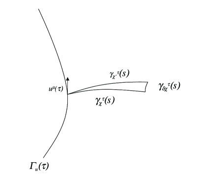
Figure 5: A sketch of the two spacelike geodesics $\mathit{\gamma}_{\chi}^{\tau}(s)$ and $\mathit{\gamma}_{\chi^{\prime}}^{\tau}(s)$ for $X^{a}$ and $X^{a}+\delta X^{b}$ respectively used in calculating spatial derivatives. The addition of $\mathit{\gamma}_{\delta\chi}^{\tau}(s)$ linking the two points defines the closed triangular region $\mathit{\Delta}$ used in Eq.$(\ref{41})$.

Then,

$$\frac{\partial N_{a}}{\partial X^{b}} = \lim_{\delta X^{b}\to 0}\frac{1}{\delta X^{b}}\left\{N_{a}(\tau,X^{a}+\delta X^{b})-N_{a}(\tau,X^{a})\right\},$$ (41)

$$= \lim_{\delta X^{b}\to 0}\frac{1}{\delta X^{b}}\left(\int_{\mathit{\gamma}_{\delta\chi}^{\tau}(s)}\bm{\omega}_{a0}-\int_{\mathit{\Delta}}\bm{d\omega}_{a0}\right),$$

where we have once again added and subtracted an integral—along $\mathit{\gamma}_{\chi_{\Delta}}^{\tau}(s)$—and used Stokes’s theorem on the closed boundary $\partial\mathit{\Delta}$ of $\mathit{\Delta}$. Parameterizing $\mathit{\Delta}$ by $\bm{d}l_{1}^{\mu}=\chi^{\mu}\bm{d}s$ and $\bm{d}l_{2}^{\mu}={\chi^{\prime}}^{\mu}\bm{d}s^{\prime}$, then

$$\partial_{b}N_{a}=\omega_{ba0}-\int_{0}^{X^{a}}R_{cba0}d\tilde{X}^{c}.$$ (42)

This equation shows explicitly the difference between taking spatial derivatives in flat spacetime verses taking derivatives in curved space. In flat spacetimes the gradient of $N_{a}$ would simply be $\omega_{ba0}$. In curved space, on the other hand, we have to take into account the differences in curvature between $X^{a}$ and $X^{a}+\delta X^{b}$, and that introduces the additional curvature term. Proceeding similarly,

$$\partial_{b}\partial_{c}N_{a} = \partial_{c}\omega_{ba0}-R_{cba0}(\tau,X^{a})+\lim_{\delta X^{c}\to 0}\frac{1}{\delta X^{c}}\int_{\mathit{\Delta}}\partial_{e}R_{dba0}\bm{d}l^{e}_{1}\wedge\bm{d}l^{d}_{2},$$ (43)

$$= \partial_{c}\omega_{ba0}-R_{cba0}(\tau,0)-\int_{0}^{X^{a}}\partial_{c}R_{eba0}d\tilde{X}^{e}.$$

From Eq. $(\ref{42})$,

$$\partial^{a}N_{a}=\omega^{a}_{\>\>\>a0}+\int_{0}^{X^{a}}R_{a0}d\tilde{X}^{a}.$$ (44)

For GWs in the TT gauge $\omega^{a}_{\>\>\>a0}={(\partial h^{a}_{a}/\partial\tau})/2=0$ and $R_{a0}=-\Box h_{a0}/2=0$, where $\Box$ is the d’Alembertian operator. $N_{a}$ is thus transverse, and $\partial^{a}N_{a}=0$. Next, from Eqs. $(\ref{43})$ and $(\ref{40})$,

$$\Box N_{a}=-\int_{0}^{X^{a}}\left(\frac{\partial R_{ab}}{\partial\tau}\right)d\tilde{X}^{b}.$$ (45)

But this also vanishes since $R_{ab}=0$. Thus, like the vector potential for EM, $N_{a}$ is a transverse vector field obeying the wave equation $\Box N_{a}=0$.

Next, to construct the effective “electric” and “magnetic” fields from $N_{a}$, we consider the four-vector $N_{A}$, constructed from $N_{a}$ with $N_{0}\equiv 0$, much like the vector potential for EM in the Coulomb gauge. Then clearly $\partial^{A}N_{A}=0$, and $N_{A}$ is a transverse field. We then define an effective field strength $\mathfrak{F}_{AB}=\partial_{A}N_{B}-\partial_{B}N_{A}$ with the corresponding “electric” and “magnetic” fields

$$\mathfrak{E}_{a} \equiv \mathfrak{F}_{a0}=-\frac{\partial N_{a}}{\partial\tau},$$

$$\mathfrak{B}^{a} \equiv \frac{1}{2}\epsilon^{abc}\mathfrak{F}_{bc}=\epsilon^{abc}\partial_{b}N_{c}.$$ (46)

Using the same methods as above, we see that

$$\frac{\partial\mathfrak{E}_{a}}{\partial\tau} = \int_{0}^{X^{a}}\left(\frac{\partial R_{b0a0}}{\partial\tau}\right)d\tilde{X}^{b},$$

$$\partial_{b}\mathfrak{E}_{a} = R_{b0a0}(\tau,0)+\int_{0}^{X^{a}}\partial_{b}R_{c0a0}d\tilde{X}^{c},$$

$$\frac{\partial\mathfrak{B}^{a}}{\partial\tau} = -\int_{0}^{X^{a}}\epsilon^{abc}\left(\frac{\partial R_{ebc0}}{\partial\tau}\right)d\tilde{X}^{e},$$

$$\partial_{b}\mathfrak{B}^{a} = -\epsilon^{afc}R_{bfc0}(\tau,0)-\int_{0}^{X^{a}}\epsilon^{afc}\partial_{b}R_{efc0}d\tilde{X}^{e},$$ (47)

Now, it is clear that by definition $\epsilon^{ABCD}\partial_{B}\mathfrak{F}_{CD}=0$, and this relation must explicitly hold if $\mathfrak{F}_{AB}$ has been defined consistently. To verify this, we first consider

$$\partial^{a}{\mathfrak{B}_{a}}=-\epsilon^{afc}R_{afc0}(\tau,0)-\int_{0}^{X^{a}}\epsilon^{afc}\partial_{a}R_{efc0}d\tilde{X}^{e}=0,$$ (48)

which vanishes identically using the 1st (Eq. $(\ref{66})$) and 2nd Bianchi Identities (Eq. $(\ref{67})$). Similarly,

$$\frac{\partial\mathfrak{B}^{a}}{\partial\tau}-\epsilon^{abc}\partial_{b}\mathfrak{E}_{c}=\epsilon^{abc}\int_{0}^{X^{a}}d\tilde{X}^{e}\left(-\frac{\partial R_{ebc0}}{\partial\tau}+\partial_{b}R_{e0c0}\right),$$ (49)

also vanishes for the same reason. Thus, $\epsilon^{ABCD}\partial_{B}\mathfrak{F}_{CD}\equiv 0$ is as a direct consequence of the Bianchi Identities for the Riemann curvature tensor.

For the other part of Maxwell’s equations, $\partial^{A}\mathfrak{F}_{AB}=0$, we consider

$$\partial^{a}\mathfrak{E}_{a}=-R_{00}(\tau,0)+\int_{0}^{X^{a}}\partial^{a}R_{c0a0}d\tilde{X}^{c}.$$ (50)

From Eq. $(\ref{67})$,

$$0=\partial^{A}R_{C00A}+\partial_{c}R_{00}-\frac{\partial R_{0C}}{\partial\tau}.$$ (51)

Once again, $R_{AB}=0$ implies that $\partial^{a}\mathfrak{E}_{a}=0$. Finally, we consider

$$\epsilon^{abc}\partial_{b}\mathfrak{B}_{c}+\frac{\partial\mathfrak{E}^{a}}{\partial\tau}=-\int_{0}^{X^{a}}\left(\frac{\partial R^{a}_{\>\>\>b}}{\partial\tau}\right)d\tilde{X}^{b}=0,$$ (52)

using Eq. $(\ref{67})$ and $R_{ab}=0$ once again. Consequently, $\mathfrak{E}_{a}$ and $\mathfrak{B}^{a}$ satisfy equations that have the same form as Maxwell’s equations. Notice also that like EM waves, $\partial^{A}\mathfrak{F}_{AB}=0$ only in the absence of sources.

The surprising connection between $\mathfrak{E}_{a}$ and $\mathfrak{B}^{a}$, and Maxwell’s equations can be understood by looking at the “electric” and “magnetic” parts of the Weyl tensor $C_{ABCD}$. For GWs propagating in a flat background, $C_{ABCD}=R_{ABCD}$ and the Riemann curvature tensor can be separated into two parts de Felice and Clarke (1990): The electric part,

$$E_{ab}\equiv-C_{0a0b}=-R_{0a0b},$$ (53)

and the magnetic part,

$$H^{a}_{\>\>b}=\frac{1}{2}\epsilon^{0aef}C_{ef0b}=-\frac{1}{2}\epsilon^{aef}R_{efb0}.$$ (54)

Clearly

$$\mathfrak{E}_{a}=-\int_{0}^{X^{a}}E_{ab}d\tilde{X}^{b},\qquad\mathfrak{B}^{a}=-\int_{0}^{X^{a}}H^{a}_{b}d\tilde{X}^{b}.$$ (55)

$\mathfrak{E}_{a}$ and $\mathfrak{B}^{a}$ are simply path integrals of $E_{ab}$ and $H^{a}_{\>\>b}$; they obey Maxwell’s equations because $E_{ab}$ and $H^{a}_{\>\>b}$ obey tensor Maxwell-like equations de Felice and Clarke (1990).

If $N_{a}$ functions as an effective vector potential for the GW, what, then, is the corresponding gauge group? Notice that although we have chosen a specific coordinate system—and thus broken general coordinate invariance—we still have a residual invariance left over. To see this, let us do a local Lorentz transformation $L_{A}^{\>\>\>\>\tilde{A}}$ on $e_{a}^{\>\>\>\>\mu}$ such that $\eta_{AB}=L_{A}^{\>\>\>\>\tilde{A}}L_{B\tilde{A}}$ while $e_{A}^{\>\>\>\>\mu}=L_{A}^{\>\>\>\>\tilde{A}}e_{\tilde{A}}^{\>\>\>\>\mu}$. This leaves $g_{\mu\nu}=e_{A\mu}\>\>e^{A}_{\>\>\>\>\nu}=e_{\tilde{A}\mu}\>\>e^{\tilde{A}}_{\>\>\>\>\nu}$ invariant, and we see that local Lorentz invariance is still left over. Now, it is straightforward to show that under a local Lorentz transformation $\omega_{CAB}\to\omega_{\tilde{C}\tilde{A}\tilde{B}}+L^{D}_{\tilde{B}}\partial_{\tilde{C}}L_{D\tilde{A}}$; $\omega_{CAB}$ transforms anomalously under a local Lorentz transformation. Consequently,

$$N_{a}\to N_{\tilde{a}}+\int_{0}^{X^{a}}L^{D}_{\>\>\>\>\tilde{0}}\partial_{\tilde{c}}L_{D\tilde{a}}d\tilde{X}^{\tilde{c}}.$$ (56)

Because we are working in the nonrelativistic limit, the gauge group for $N_{a}$ is the local Galilean group. Indeed, for a pure boost in the nonrelativistic limit, $L_{A\tilde{A}}\approx\delta_{A\tilde{A}}-v_{a}K^{a}_{A\tilde{A}}$ where $K^{a}_{A\tilde{A}}$ is the generator of boosts. Then,

$$N_{a}\to N_{\tilde{a}}-\int_{0}^{X^{a}}dv_{\tilde{a}}=N_{\tilde{a}}-\left\{v_{\tilde{a}}(\tau,X^{a})-v_{\tilde{a}}(\tau,0)\right\},$$ (57)

and $N_{a}$ changes by a local velocity field.

Finally, we calculate the equations of motion for the test particle in a GW. Equation $(\ref{26})$ for GWs is

$${\mathcal{L}}=\frac{m}{2}\left(\frac{dX^{a}}{d\tau}-N^{a}\right)^{2}+qA_{0}+qA_{a}\left(\frac{dX^{a}}{d\tau}-N^{a}\right),$$ (58)

from which we get

$$m\frac{d^{2}X^{a}}{d\tau^{2}}=-m\left\{\mathfrak{E}^{a}+\epsilon^{abc}\frac{dX_{b}}{d\tau}\mathfrak{B}_{c}\right\}+q\left\{E^{a}+\epsilon^{abc}\frac{dX_{b}}{d\tau}B_{c}\right\},$$ (59)

after using Eq. $(\ref{47})$; like DeWitt we drop terms $O(Ah)$. In Section II we stated that we would neglect terms of order $(c^{A}-\delta^{A}_{0})h_{ab}$, and yet Eq. $(\ref{60})$ contains just such a term. It is, however, straightforward, though tedious, to repeat the calculation for Eq. $(\ref{60})$ keeping the next higher order velocity-connection terms. After doing so we still obtain the above to lowest order.

Let us suppose that a GW can be approximated as a plane wave with wave vector $k_{a}$. Notice that the integral in Eq. $(\ref{26})$ is always over the plane perpendicular to $k_{a}$, yet $h_{ab}$ is a only function of the spatial coordinates parallel to $k_{a}$. Consequently, $N_{a}=\omega_{ba0}X^{b}$, $\mathfrak{E}_{a}=R_{b0a0}X^{b}$ and $\mathfrak{B}^{a}=\epsilon^{abc}R_{bce0}X^{e}/2$. Thus, for planar GWs,

$$m\frac{d^{2}X_{a}}{d\tau^{2}}=-m\left\{R_{b0a0}X^{b}+\frac{dX^{b}}{d\tau}X^{c}R_{abc0}\right\}+q\left\{E_{a}+\epsilon_{abc}\frac{dX^{b}}{d\tau}B^{c}\right\}.$$ (60)

As expected, in the low velocity limit where the $\mathfrak{B}^{a}$ term can be neglected, this is just the geodesic deviation equation for a charged test particle. Note also that Eq. $(\ref{61})$ holds for general GWs in the long-wavelength limit as well, and that it agrees with the equation of motion for a charged test particle interacting with a GW found in Misner et al. (1973).

V Concluding Remarks

In Eqs. $(\ref{26})$ and $(\ref{28})$ we can clearly see the natural separation that occurs in the dynamics of test particles in two extremes. In the one extreme the metric for $\mathbb{M}$ can be approximated as being stationary. Matter moving with a characteristic velocity $v$ much smaller than the speed of light ($v/c<<1$) makes up the dominant contribution to the stress-energy tensor in these spacetimes; thus to a very good approximation the presence of GWs can be neglected. In this extreme our Hamiltonian reduces to DeWitt’s Hamiltonian, and the straightforward approach to the derivation of $H_{SF}$ described in the Introduction works. In the other extreme, all the curvature effects are due to GWs, and the characteristic velocity for the metric is the speed of light. In this extreme, our Hamiltonian reduces to the Hamiltonian derived in Speliotopoulos (1995) for geodesic deviation motion in the presence of GW’s in the long-wavelength limit, and the equations of motion reduce to the usual geodesic deviation equations of Misner et al. (1973).

Let us be very clear. The dynamics of nonrelativistic, classical test particles in stationary spacetimes that we have derived in the GLF and are the same as the dynamics for these particles derived using standard methods. Thus, such classical tests of GR as the perihelion of Mercury and the gravitational redshift will follow through in the GLF as well. By extension, because QFCS’s are usually formulated in stationary spacetimes, we would expect such an analysis as the evaporation of black holes and black hole thermodynamics to hold also. It is when we consider nonstationary spacetimes—such as those where GWs play a dominant role in determining the physics—that we must take care to explicitly include the observer and his experimental apparatus in the analysis.

Traditionally, there is an almost linear progression of approximations, such as the hierarchy sketched in Fig. 6a, that we usually associated with GR. Within full GR we can make the linearized gravity approximation, which is thought to be inclusive of both the parametrized-post-Newtonian Misner et al. (1973) (stationary) and the GW (nonstationary) limits (see also Forward (1961) and Braginsky (1977)). We can, with further restrictions, then pass over to either the parametrized-post-Newtonian (PPN) limit or the GW limit within this linearized approximation. Based on the arguments above and the results of our analysis in this paper, we find the separation between the PPN and GW limits to occur at a much higher level; the dynamics of particles in stationary spacetimes is drastically different from that in nonstationary spacetimes. This conclusion is consistent with Hawking and Ellis (1973), Birrell and Davies (1982) and Wald (1994), all of whom note differences between dynamical theories in stationary versus nonstationary spacetimes. Thus, instead of the standard formulation consisting of the linear sequence of approximations in Fig. 6a, we should, as shown in Fig. 6b, instead separate the dynamics in stationary versus nonstationary spacetimes from the start.

Figure 6: Fig. 6a is a schematic of the hierarchy of approximations that we usually associate with GR. Fig. 6b is the modified hierarchy based on the results of this paper. Notice the explicit separation between stationary and nonstationary spacetimes from the start.

What is most surprising about our results is the form that the coupling of general GWs to the test particle takes in the GLF. The tidal nature of the force that a GW induces on a test particle introduces an effective velocity field $N_{a}$ to the system that couples vectorially, under the Lorentz Group, to the particle, even though the GW itself is a rank-2 tensor. This $N_{a}$—being a path integral—is in general a nonlocal function of the of Ricci coefficients, although for planar GWs it reduces to the product of the Ricci coefficient and the position of the test particle. [A vector coupling of GWs to matter was proposed by one of the present authors (R.Y.C.) in Chiao (2002) based on a generalization of the PPN formalism.] Thus the motion of the test particle is determined by the cumulative effects of the GW along the distance between the observer’s worldline and the test particle’s. Like the vector potential for EM, $N_{a}$ is a transverse field satisfying the wave equation, and like EM, effective electric $\mathfrak{E}$ and magnetic $\mathfrak{B}$ fields can also be constructed from $N_{a}$ that obey equations that have the same form as Maxwell’s equations. Thus, $N_{a}$ functions as a vector potential for $\mathfrak{E}$ and $\mathfrak{B}$ with its gauge group being the local Galilean group. Indeed, the equations of motion for the test particle in the presence of arbitrary GWs has the form of the Lorentz force with the mass $m$ of the particle playing the role of the “charge.”

Surprising though this vector coupling may be at first glance, after further study we see that there are deep connections between $N_{a}$ and the tetrad formulation of eneral relativity. $\mathfrak{E}$ and $\mathfrak{B}$ are proportional to the path integrals of the electric $E_{ab}$ and magnetic $H_{ab}$ parts of the Weyl tensor, respectively, and it is precisely the Weyl tensor that contains GW excitations. It is also known that $E_{ab}$ and $H_{ab}$ obey tensor Maxwell’s equations for GWs propagating on a flat, source-free background, and the fact that $\mathfrak{E}$ and $\mathfrak{B}$ satisfy Maxwell’s equations is simply the reflection that $E_{ab}$ and $H_{ab}$ do. In fact, the identity $\epsilon^{ABCD}\partial_{B}\mathfrak{F}_{CD}=0$ holds precisely because of the 1st and 2nd Bianchi conditions for the Riemann curvature tensor, while $\partial^{A}\mathfrak{F}_{AB}=0$ only holds because we are in a source-free region for GWs. As for $N_{a}$ itself, it is precisely “half” of the loop integral of the real part of Ashtekar’s connection in the loop-variable formulation of quantum gravity. Indeed, Ashtekar’s loop integrals can be thought of as quantum corrections to the “classical” $N_{a}$ presented here Ashtekar (1988).

Since $N_{a}$ is a nonlocal object, it is natural to question the practicality of Eq. $(\ref{60})$ as compared to, say, Eq. $(\ref{61})$, whose form for long-wavelength GWs is well known. Indeed, it would seem that for Earth-based systems the long-wavelength version of Eq. $(\ref{61})$ would be sufficient to describe all physically interesting systems. We note, however, that at $4$ km the arms of LIGO are comparable to the reduced wavelength of the GWs for GWs with a frequency of 10 khz, which is at the upper limits of LIGO’s frequency response spectrum LIGO-Report ; measurements of the spatial variation of GWs are becoming experimentally accessible. Similarly, when LISA’s (Laser Interferometer Space Antenna) arm lengths begins to approach the reduced wavelengths of GWs in the high-frequency limit of its sensitivity, the concept of the $N_{a}$ field and the GLF becomes essential. For these arbitrary GWs, Eq. $(\ref{60})$ instead of Eq. $(\ref{61})$ must be used. Since it is $N_{a}$ in general that will be measured, and not $h_{ab}$, it is an interesting, and important, question as to how much information about $h_{ab}$ can be obtained from measurements of $N_{a}$.

While most of our focus has been on classical dynamics, we end this paper by looking at a gedanken experiment that probes the essential difference between the classical and quantum dynamics of nonrelativistic test particles in the linearized gravity limit. Extension of Eq. $(\ref{37})$ to quantum mechanics is straightforward. For nonrelativistic, neutral particles with wave function $\psi$,

$$i\hbar\frac{\partial\psi}{\partial t}=-\frac{\hbar^{2}}{2m}\nabla^{2}\psi-i\hbar N_{a}\partial^{a}\psi.$$ (61)

Notice that the interaction term $N_{a}\partial^{a}\psi$ has the same form as the coupling of an EM vector potential $A_{B}$ (expressed in GLF coordinates) to a charge particle coupled to weak EM fields. In the EM case, the solution of equations of this form leads, on the quantum level, to the Aharonov-Bohm effect, which is expressible through Yang’s nonintegrable phase factor (Wilson loop) Yang (1975) $\lambda_{EM}=\exp\{i(e/\hbar)\oint A_{B}dX^{B}\}$. In direct analogy, Eq. $(\ref{a})$ suggests that like the EM case, a time-dependent Aharanov-Bohm interference experiment such as those described in Stodolsky (1979) or Anandan (1979) can in principle be done, but now with GWs. We would expect this to lead to a corresponding phase factor for gravity $\lambda_{GR}=\exp\{i(m/\hbar)\oint N_{A}dX^{A}\}$. While actually performing this experiment would be unrealistic at this time, the corresponding gedanken experiment does illustrate both the essential difference between the classical and quantum systems, and the importance of this gravitational nonintegrable phase factor.

Consider the gedanken Aharanov-Bohm-type experiment shown in Fig. 7 using a Gaussian GW packet with a width $l_{GW}$ at some time $t_{I}$. Fig. 7a shows the spacetime diagram for the particle and the GW used in the interferometry experiment with a time slice drawn in at $t_{I}$. A schematic of the corresponding physical apparatus at this time slice is shown in Fig.7b. We require that the GW also be an unipolar wave packet so that at all times the amplitude of the $\mathfrak{E}$ and $\mathfrak{B}$ for the packet is non-negative. The interfering particle is taken to be a Gaussian wave packet as well, but with width $l_{p}$ at any time $t$. After being emitted at the source, the particle at event $p_{A}$ passes through the first beam splitter shown in Fig. 7b, and there is a finite probability amplitude it will propagate either along $\mathit{\Gamma}^{1}$ or along $\mathit{\Gamma}^{2}$ until it is is recombined at event $p_{B}$. It is impossible, even in principle, to know which path the particle took through the interferometer. As usual, the combined path $\mathit{\Gamma}=\mathit{\Gamma}^{1}\cup\mathit{\Gamma}^{2}$ encircles the GW beam.

The Bonse-Hart interferometer of a type shown in Fig. 7b is a concrete example of an interferometer that could be used in this experiment; in this case the interfering particle could be neutrons. The gray oval patch at the center of the interferometer represents the time slice at $t_{I}$ shown in Fig. 7a of the Gaussian beam waist. Most importantly, we choose the size of the interferometer such that $R>>l_{GW}+l_{p}$ where $R$ is the distance from the center of the GW beam in Fig. 7b to each arm of the interferometer. Thus, on a classical level the GW and the neutron worldlines do not intersect, and therefore the neutron feels no forces at any time arising from the GW. On a quantum mechanical level, the amplitude of the neutron’s wave function is exponentially small where the amplitude of the GW is large, and the amplitude of the GW is exponentially small where the amplitude of the wave function is large.

Although the wave function of the neutrons satisfy Eq. $(\ref{a})$, because they are Gaussian wave packets we can make a WKB-like approximation by taking $\psi\approx e^{i\Theta}$. For $h_{ab}$ with small spatial variations along the worldlines, Eq. $(\ref{a})$ reduces to

$$0=\frac{\partial\Theta}{\partial t}+N_{a}\partial^{a}\Theta,$$ (62)

where we have neglected terms $\mathcal{O}(|\nabla\Theta|^{2})$ since $N_{a}$ is small. The solution of Eq. $(\ref{b})$ in the linearized gravity limit for the particle propagating along worldline $\mathit{\Gamma}^{1}$ is

$$\Theta_{\mathit{\Gamma}^{1}}=\frac{m}{\hbar}\int_{\mathit{\Gamma}^{1}}N_{A}dX^{A},$$ (63)

from Eq. $(\ref{75})$ of Appendix B. Similarly, if the particle had traveled the worldline $\mathit{\Gamma}^{2}$,

$$\Theta_{\mathit{\Gamma}^{2}}=\frac{m}{\hbar}\int_{\mathit{\Gamma}^{2}}N_{A}dX^{A}.$$ (64)

The phase factor

$$\exp\{i\Delta\Theta\}\equiv\exp\left\{\Theta_{\mathit{\Gamma}^{1}}-\Theta_{\mathit{\Gamma}^{2}}\right\}=\exp\left\{i\frac{m}{\hbar}\int_{\mathit{\Gamma}}N_{A}dX^{A}\right\},$$ (65)

is a measure of the phase difference between the particle propagating along $\mathit{\Gamma}^{1}$ versus propagating along $\mathit{\Gamma}^{2}$. Equation $(\ref{e})$ is simply the $\lambda_{GR}$ that we predicted above. Next, since $\mathit{\Gamma}$ is a closed loop, by the Stokes’s theorem,

$$\exp\{i\Delta\Theta\}=\exp\left\{i\frac{m}{\hbar}\int_{\mathcal{D}}\mathfrak{F}_{AB}dX^{A}\wedge dX^{B}\right\},$$ (66)

where $\mathcal{D}$ is the surface bound by $\mathit{\Gamma}$ and we have used the definition of $\mathfrak{F}_{AB}$. Because the boundary of $\mathcal{D}$ is made up of timelike curves, from Eqs. $(\ref{47})$, $(\ref{54})$, and $(\ref{56})$ the dominant contribution to the surface integral in Eq. $(\ref{f})$ comes from $R_{0a,0b}$. As expected, the phase factor depends on the Riemann curvature tensor, and is independent of coordinate choice, even though Eq. $(\ref{a})$ is dependent on the gauge-dependent field $N_{a}$.

We note also the underlying topological nature of Fig. $\ref{Fig_8}a$. If a path $\mathit{\Gamma}$ is chosen that does not encircle the GW beam, $\Delta\Theta=0$; if it does, $\Delta\Theta\neq 0$. $\mathit{\Gamma}$ cannot be shrunk to zero without cutting though the GW beam, and thus altering the topology of the $\mathit{\Gamma}$-GW beam system. Moreover, each time one goes around $\mathit{\Gamma}$, the phase difference $\Delta\Theta$ changes by an integral multiple of the same factor; $\Delta\Theta$ is thus proportional to the linking number of $\mathit{\Gamma}$ around the GW beam. That $\Delta\Theta$ is related to the linking number is not unexpected since $N_{a}$ is related to Ashtekar’s loop variables. Nonetheless, it does point out the possibility of doing experiments such as Tonomura (1998) that directly measures the linking number of $\mathit{\Gamma}$, and this indicates the underlying topological nature of this gravitational Aharonov-Bohm-type effect.

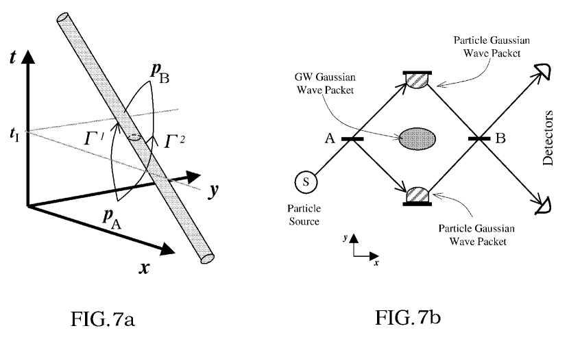
Figure 7: Fig. 7a is a sketch of spacetime diagram showing the passage of the unipolar, Gaussian GW (shown in gray) and the worldlines of two particles beams, along the two paths $\mathit{\Gamma}^{1}$ and $\mathit{\Gamma}^{2}$ (i. e. the two dominant Feynman paths), of the interferometer encircling it. Events $p_{A}$ and $p_{B}$ correspond to the splitting and recombining of the initial and final beam splitters shown in Fig. 7a. Fig. 7b shows a schematic of a possible experimental set-up (a Bonse-Hart interferometer) at the given time slice $t_{I}$ shown in Fig. 7a. The GW beam passes through the center of the Bonse-Hart interferometer, and the gray oval shows the cross section of the Gaussian beam waist which forms at the center of the plane of the interferometer.

Appendix A Review of Linearized Gravity and Tetrad Formalisms

In this appendix, we present a brief review of some of the properties of general tetrad frames, differential forms, and linearized gravity that we shall need. The review is not exhaustive and the reader is referred to Wald (1984) or de Felice and Clarke (1990) for a more complete presentation.

A tetrad is a local coordinate system formed by a set of four orthonormal vectors $\{e_{A}^{\>\>\>\>\mu}\}$ such that $e_{A}^{\>\>\>\>\mu}e_{B\mu}=\eta_{AB}$ and $e^{A}_{\>\>\>\>\mu}e_{A\nu}=g_{\mu\nu}$. These $\{e_{A}^{\>\>\>\>\mu}\}$ do not have to be tied to any observer’s worldline as we have done in the above, and the results presented here are valid in general.

Since $e_{A}^{\>\>\>\>\nu}$ is a unit vector, the covariant derivative $\nabla_{\mu}e_{B\nu}$ can only be a rotation or boost of $e_{B}^{\>\>\>\>\nu}$. This “rotation matrix” is determined by the Ricci rotation coefficients:

$$\omega_{CAB}=e_{C}^{\>\>\>\>\mu}e_{A}^{\>\>\>\>\nu}\nabla_{\mu}e_{B\nu},$$ (67)

with $\omega_{CAB}=-\omega_{CBA}$. It is straightforward to show that in a tetrad frame,

$$R_{ABCD}= e_{A}^{\>\>\>\>\mu}\partial_{\mu}\omega_{BCD}-e_{B}^{\>\>\>\>\mu}\partial_{\mu}\omega_{ACD}-$$ (68)

$$\left\{\omega_{AFC}\omega_{B}{}^{F}_{\>\>\>\>D}-\omega_{BFC}\omega_{A}{}^{F}_{\>\>\>\>D}+\omega_{AFB}\omega^{F}_{\>\>\>\>CD}-\omega_{BFA}\omega^{F}_{\>\>\>\>CD}\right\}.$$

We emphasize that objects with capital Roman indices in the tetrad frame—such as $\omega_{CAB}$—are scalars. They only take the partial derivative, and not the covariant derivative.

Given a tetrad frame, it is natural to work with differential forms, which we shall denote by symbols in boldface. As $1$-forms we have $\bm{e}_{A}\equiv e_{A\mu}\bm{d}x^{\mu}$ and $\bm{\omega}_{AB}=\omega_{\mu AB}\bm{d}x^{\mu}$, and as 2-forms we have $\bm{R}_{AB}\equiv R_{\mu\nu AB}\bm{d}x^{\mu}\wedge\bm{d}x^{\nu}/2$. As usual, $\bm{d}$ is the exterior derivative. Equation $(\ref{62})$ then becomes

$$\bm{de}_{A}=\bm{e}^{B}\wedge\bm{\omega}_{AB},$$ (69)

where $\wedge$ is the wedge product; $\bm{\omega}_{AB}$’s role as a “rotation” or boost matrix is now manifest. Equation $(\ref{63})$ is then

$$\bm{R}_{A}^{\>\>\>\>B}=\bm{d\omega}_{A}^{\>\>\>\>B}+\bm{\omega}_{A}^{\>\>\>\>C}\wedge\bm{\omega}_{C}^{\>\>\>\>B}.$$ (70)

Taking the exterior derivative of Eq. $(\ref{64})$, we get the 1st Bianchi identity,

$$0=\bm{e}_{B}\wedge\bm{R}_{A}^{\>\>\>\>B},$$ (71)

and the exterior derivative of Eq. $(\ref{66})$ gives the 2nd Bianchi identity

$$\bm{dR}_{A}^{\>\>\>\>B}=\bm{R}_{A}^{\>\>\>\>C}\wedge\bm{\omega}_{C}^{\>\>\>\>B}-\bm{\omega}_{A}^{\>\>\>\>C}\bm{R}_{C}^{\>\>\>\>B}.$$ (72)

In the case of linearized gravity, $g_{\mu\nu}=\eta_{\mu\nu}+h_{\mu\nu}$ where $h_{\mu\nu}$ is “small”, and we are only concerned with terms linear in $h_{\mu\nu}$. Then $g^{\mu\nu}=\eta^{\mu\nu}-h^{\mu\nu}$ where on the left hand side we use $\eta_{\mu\nu}$ to raise and lower indices. In this limit

$$\Gamma^{\alpha}_{\mu\nu} = \frac{1}{2}\left(\partial_{\mu}h_{\nu}^{\alpha}+\partial_{\nu}h^{\alpha}_{\mu}-\partial^{\alpha}h_{\mu\nu}\right),$$

$$R^{\mu}_{\>\>\>\>\nu\alpha\beta} = \frac{1}{2}\left\{\partial_{\nu}(\partial_{\alpha}h_{\beta}^{\mu}-\partial_{\beta}h_{\alpha}^{\mu})+\partial^{\mu}(\partial_{\beta}h_{\nu\alpha}-\partial_{\alpha}h_{\nu\beta})\right\},$$

$$R_{\mu\nu} = -\frac{1}{2}\Box h_{\mu\nu}+\frac{1}{2}\partial_{\mu}\partial^{\alpha}h_{\alpha\nu}+\frac{1}{2}\partial_{\nu}\partial^{\alpha}h_{\alpha\mu}-\frac{1}{2}\partial_{\mu}\partial_{\nu}h_{\alpha}^{\alpha},$$

$$R = -\Box h_{\mu}^{\mu}+\partial_{\mu}\partial_{\nu}h^{\mu\nu}.$$ (73)

For GWs in the TT gauge, $h_{\mu}^{\mu}=0$, $\partial^{\mu}h_{\mu\nu}=0$, and $h_{0\mu}=0$, so that $R=0$, $R_{0\mu}=0$, and the equation of motion for GWs is $R_{\hat{a}\hat{b}}=-\Box h_{\hat{a}\hat{b}}/2=0$.

To construct the tetrad frame for linearized gravity, we first note that in flat spacetime the tetrad frame is trivial: $\{\delta_{A}^{\mu}\}$. The presence of small $h_{\mu\nu}$ rotates these vectors and

$$e_{A}^{\>\>\>\>\mu}=\left(\delta^{\mu}_{\nu}-\frac{1}{2}h^{\mu}_{\nu}\right)\delta_{A}^{\nu},\qquad e^{A}_{\>\>\>\>\mu}=\left(\delta_{\mu}^{\nu}+\frac{1}{2}h_{\mu}^{\nu}\right)\delta^{A}_{\nu}.$$ (74)

Note that this choice is not unique. As noted in Sec. IV 4, given any tetrad frame, we can always do a local Lorentz transformation that will still preserve the orthonormality of $\{e_{A}^{\>\>\>\>\mu}\}$. The choice we have made for $\{e_{A}^{\>\>\>\>\mu}\}$ for the GLF, and used in the construction in Sec. I, corresponds to an observer at rest in his proper frame.

Using Eq. $(\ref{62})$ and the Levi-Civita connection in Eq. $(\ref{68})$, we find that

$$\omega_{CAB}=-\frac{1}{2}\left(\partial_{A}h_{BC}-\partial_{B}h_{AC}\right),$$ (75)

while $R_{ABCD}=\partial_{A}\omega_{BCD}-\partial_{B}\omega_{ACD}$ in the linearized gravity limit. Also in this limit, the equations for the Ricci tensor and scalar in Eq. $(\ref{68})$ have the same form in the tetrad frame, with the replacement of Greek indices by capital Roman indices.

Appendix B Phase Factor Solution

Equation $(\ref{b})$ is a quasi-linear partial differential equation Zwillinger (1998) whose method of solution is well known. First, both $t$ and $X^{a}$ are considered functions of a parameter $\tau$, so that $\Theta=\Theta(t(\tau),X^{a}(\tau))$, and defines a constant surface in $(t,X^{a})$ space. Consequently,

$$0=\frac{dt}{d\tau}\frac{\partial\Theta}{\partial t}+\frac{dX^{a}}{d\tau}\partial_{a}\Theta,$$ (76)

and for Eq. $(\ref{71})$ to be a solution of Eq. $(\ref{b})$,

$$\frac{\partial t}{\partial\tau}=1,\qquad\frac{dX^{a}}{d\tau}=N^{a};$$ (77)

the quasi-linear partial differential equation reduces to the solution of a set of ordinary differential equations. Although Eq. $(\ref{72})$ can be solved using standard methods once an initial condition is given, the underlying physics become much clearer if we consider instead the following function

$$\Theta_{\widetilde{\mathit{\Gamma}}}(t(T),X^{a}(T))=\frac{m}{\hbar}\int_{\widetilde{\mathit{\Gamma}}}N_{A}(t(\tau),X^{a}(\tau))dX^{A},$$ (78)

where the integral is from a fixed point $(t(0),X^{a}(0))$ to the point $(t(T),X^{a}(T))$ along $\widetilde{\mathit{\Gamma}}$. The prefactor $m/\hbar$ is included so that $\Theta_{\widetilde{\mathit{\Gamma}}}$ is unitless. We choose $\widetilde{\mathit{\Gamma}}$ such that its tangent vector is given by Eq. $(\ref{72})$, and we parameterize it by $\tau\in[0,T]$. $\widetilde{\mathit{\Gamma}}$ starts at the point $(t(0),X^{a}(0))$, and is used also as the initial condition for Eq. $(\ref{72})$. Clearly,

$$\frac{d\Theta_{\widetilde{\mathit{\Gamma}}}(t,X^{a})}{d\tau}=\frac{m}{\hbar}N_{A}\frac{dX^{A}}{d\tau}=\frac{m}{\hbar}N_{a}N^{a}\approx 0,$$ (79)

in the linearized gravity limit, while the left-hand-side vanishes identically from Eq. $(\ref{71})$. Thus, $\Theta_{\widetilde{\mathit{\Gamma}}}(t,X^{a})$ is a solution of Eq. $(\ref{b})$. Because it is path dependent, this solution is not unique, however.

The spatial component of the tangent vector to $\widetilde{\mathit{\Gamma}}$ lies along $N_{a}$, and for plane waves, $N_{a}$ is perpendicular to the direction of propagation. Thus, for the Gaussian beam in Fig. $\ref{Fig_8}a$, $\widetilde{\mathit{\Gamma}}$ will wrap around the beam. We can, of course, go around this beam either in a clockwise or counterclockwise direction, and we denote a clockwise path by $\widetilde{\mathit{\Gamma}}^{-}$ and a counterclockwise path by $\widetilde{\mathit{\Gamma}}^{+}$. To $\widetilde{\mathit{\Gamma}}^{-}$ there is then the corresponding the function $\Theta_{\widetilde{\mathit{\Gamma}}^{-}}$, and to $\widetilde{\mathit{\Gamma}}^{-}$ there is the corresponding function $\Theta_{\widetilde{\mathit{\Gamma}}^{+}}$.

Consider now the functions

$$\Theta_{\mathit{\Gamma}^{1}}(t(T),X^{a}(T)) = \frac{m}{\hbar}\int_{\mathit{\Gamma}^{1}}N_{A}dX^{A},$$

$$\Theta_{\mathit{\Gamma}^{2}}(t(T),X^{a}(T)) = \frac{m}{\hbar}\int_{\mathit{\Gamma}^{2}}N_{A}dX^{A},$$ (80)

and we restrict ourselves to those $\widetilde{\mathit{\Gamma}}^{\pm}$ that lie on the surface of the beam, meaning that $\widetilde{\mathit{\Gamma}}^{\pm}$ do not come closer than $l_{GW}$ to the center of the beam of GWs. Because $N_{a}$ is exponentially small outside of the Gaussian beam, $\Theta_{\mathit{\Gamma}^{1}}\approx\Theta_{\widetilde{\mathit{\Gamma}}^{+}}$ and $\Theta_{\mathit{\Gamma}^{2}}\approx\Theta_{\widetilde{\mathit{\Gamma}}^{-}}$. Thus, Eqs. $(\ref{75})$ are solutions of Eq. $(\ref{b})$.