Gravitational Waves from Perturbed Black Holes and Relativistic Stars

Abstract

These lectures aim at providing an introduction to the properties of gravitational waves and in particular to those gravitational waves that are expected as a consequence of perturbations of black holes and neutron stars. Imprinted in the gravitational radiation emitted by these objects is, in fact, a wealth of physical information. In the case of black holes, a detailed knowledge of the gravitational radiation emitted as a response to perturbations will reveal us important details about their mass and spin, but also about the fundamental properties of the event horizon. In the case of neutron stars, on the other hand, this information can provide a detailed map of their internal structure and tell us about the equation of state of matter at very high density, thus filling-in a gap in energies and densities that cannot be investigated by experiments in terrestrial laboratories.

Keywords: Gravitational Waves, Black Holes, Neutron Stars, Perturbations, Oscillations.

PACS numbers: 04.30.-w –  04.70.-s –  97.60.Jd –  31.15.Md –  04.40.Dg.

1 A Brief Introduction to Gravitational Waves

Being prepared for a Summer School, these lecture notes are meant principally as a first introduction to the rather vast and rapidly growing area of research that deals with gravitational waves. As a result, these notes will simply provide the basic concepts of this field of research and briefly review the most important results. The bibliography is not meant to be complete and the sparse references are used mostly as pointers to review articles where the topics of these lectures find a more detailed discussion and where a complete presentation of the literature can be found. In what follows I will assume that the reader is proficient in basic tensor algebra, is familiar with the fundamental concepts in General Relativity and has already encountered a black hole solution to Einstein equations.

The lecture notes are organized in three main parts. In the first one, I rapidly introduce the basic properties of gravitational waves by deriving a wave solution of the Einstein equations and discussing the sense of the transverse-traceless gauge. A brief discussion about the generation of gravitational waves will also be made. In the second part, I discuss in some detail the perturbation properties of a Schwarzschild black hole and the gravitational radiation that is expected as a result. Finally, the third part is devoted to presenting the basic elements of the theory of stellar perturbations and how stellar perturbations can be used to generate gravitational waves. The discussion will be restricted to spherical oscillations in the case of relativistic stars and to nonradial oscillations in the case of Newtonian stars. A brief classification of the modes of oscillations will also be presented together with an introduction to the onset of non-axisymmetric instabilities.

These lectures notes are taken in part from the introductory course on General Relativity given to the graduate students at SISSA and is inspired by the corresponding discussions in a number of textbooks and in particular by those in [1, 2, 3]. A space-like signature $(-,+,+,+)$ will be used, with Greek indices taken to run from 0 to 3 and Latin indices from 1 to 3. Covariant derivatives are denoted with a semi-colon and partial derivatives with a comma. Tensors are indicated with bold symbols (i.e. ${\boldsymbol{\it A}}$) and three-vectors with the standard arrow (i.e. ${\vec{A}}$). Finally, I will adopt geometrized units in which $G=c=1$. All of the figures presented here are original and have not been published elsewhere.

1.1 Linearized Einstein Equations

The starting point in discussing gravitational waves cannot but come from the Einstein field equations, expressing the close equivalence between matter-energy and curvature

$$G_{\mu\nu}\equiv R_{\mu\nu}-\frac{1}{2}g_{\mu\nu}R=8\pi T_{\mu\nu}\ .$$ (1)

In the 10 linearly independent equations (1), $R_{\mu\nu}$ and $R$ are the Ricci tensor and scalar, respectively, $g_{\mu\nu}$ and $G_{\mu\nu}$ are the metric and Einstein tensors, respectively, while $T_{\mu\nu}$ is the stress-energy tensor of the matter in the spacetime considered.

Looking at the Einstein equations (1) as a set of second-order partial differential equations it is not easy to predict that there exist solutions behaving as waves. Indeed, and as it will become more apparent in this Section, the concept of gravitational waves as solutions of Einstein equations is valid only under some rather idealized assumptions such as: a vacuum and asymptotically flat spacetime and a linearized regime for the gravitational fields. If these assumptions are removed, the definition of gravitational waves becomes much more difficult. In these cases, in fact, the full nonlinearity of the Einstein equations complicates the treatment considerably and solutions can be found only numerically. It should be noted, however, that in this respect gravitational waves are not peculiar. Any wave-like phenomenon, in fact, can be described in terms of exact “wave equations” only under very simplified assumptions such as those requiring an uniform “background” for the fields propagating as waves.

These considerations suggest that the search for wave-like solutions to Einstein equations should be made in a spacetime with very modest curvature and with a metric line element which is that of flat spacetime but for small deviations on nonzero curvature, i.e.

$$g_{\mu\nu}=\eta_{\mu\nu}+h_{\mu\nu}+{\cal O}([h_{\mu\nu}]^{2})\ ,$$ (2)

where

$$\eta_{\mu\nu}={\rm diag}(-1,1,1,1)\ ,$$ (3)

and the linearized regime is guaranteed by the fact that

$$|h_{\mu\nu}|\ll 1\ .$$ (4)

Fortunately, the conditions expressed by equations (2) and (4) are, at least in our Solar system, rather easy to reproduce and, in fact, the deviation away from flat spacetime that could be measured, for instance, on the surface of the Sun are

$$|h_{\mu\nu}|\sim|h_{00}|\simeq\frac{M_{\odot}}{R_{\odot}}\sim 10^{-6}\ .$$ (5)

Before writing the linearized version of the Einstein equations (1) it is necessary to derive the linearized expression for the Christoffel symbols. In a coordinate basis (as the one will will assume hereafter), the general expression for the affine connection is

$$\Gamma^{\mu}_{\ \alpha\beta}=\frac{1}{2}g^{\mu\nu}(g_{\nu\alpha,\beta}+g_{\beta\nu,\alpha}-g_{\alpha\beta,\nu})\ ,$$ (6)

where the partial derivatives are readily calculated as

$$g_{\nu\alpha,\beta}=\eta_{\nu\alpha,\beta}+h_{\nu\alpha,\beta}=h_{\nu\alpha,\beta}\ ,$$ (7)

so that the linearized Christoffel symbols become

$$\Gamma^{\mu}_{\ \alpha\beta} = \frac{1}{2}\eta^{\mu\nu}(h_{\nu\alpha,\beta}+h_{\beta\nu,\alpha}-h_{\alpha\beta,\nu})$$ (8)

$$= \frac{1}{2}(h^{\ \ \mu}_{\alpha\ \ ,\beta}+h^{\ \ \mu}_{\beta\ \ ,\alpha}-h^{\ \ \ ,\mu}_{\alpha\beta})\ .$$

Note that the operation of lowering and raising the indices in expression (8) is not made through the metric tensors $g_{\mu\nu}$ and $g^{\mu\nu}$ but, rather, through the spacetime metric tensors $\eta_{\mu\nu}$ and $\eta^{\mu\nu}$. This is just the consequence of linearized approximation and, despite this, the spacetime is really curved!

Once the linearized Christoffel symbols have been computed, it is possible to derive the linearized expression for the Ricci tensor which takes the form

$$R_{\mu\nu} = \Gamma^{\alpha}_{\ \mu\nu,\alpha}-\Gamma^{\alpha}_{\ \mu\alpha,\nu}$$ (9)

$$= \frac{1}{2}(h^{\ \;\alpha}_{\mu\ \;,\nu\alpha}+h^{\ \;\alpha}_{\nu\ \;,\,\mu\alpha}-h^{\ \ \ \ \;\alpha}_{\mu\nu,\,\alpha}-h_{,\,\mu\nu})\ ,$$

where

$$h\equiv h^{\alpha}_{\ \;\alpha}=\eta^{\mu\alpha}h_{\mu\alpha}\ ,$$ (10)

is the trace of the metric perturbations. The resulting Ricci scalar is then given by

$$R\equiv g^{\mu\nu}R_{\mu\nu}\simeq\eta^{\mu\nu}R_{\mu\nu}\ .$$ (11)

Making now use of (9) and (11) it is possible to rewrite the Einstein equations (1) in a linearized form as

$$h^{\ \ \ \alpha}_{\mu\alpha,\ \nu}+h^{\ \ \ \alpha}_{\nu\alpha,\ \mu}-h^{\ \ \ \alpha}_{\mu\nu,\ \alpha}-h_{,\mu\nu}-\eta_{\mu\nu}(h^{\ \ \ \alpha\beta}_{\alpha\beta,}-h^{\ \ \alpha}_{,\alpha})=16\pi T_{\mu\nu}\ .$$ (12)

Although linearized, the Einstein equations (12) do not seem yet to suggest a wave-like behaviour. A good step in the direction of unveiling this behaviour can be made if a more compact notation is introduced and which makes use of “trace-free” tensors defined as

$${\bar{h}}_{\mu\nu}\equiv h_{\mu\nu}-\frac{1}{2}\eta_{\mu\nu}h\ ,$$ (13)

where the “bar-operator” can be applied to any symmetric tensor so that, for instance, ${\bar{R}}_{\mu\nu}=G_{\mu\nu}$ and ${\bar{\bar{h}}}_{\mu\nu}=h_{\mu\nu}$. Using this notation, the linearized Einstein equations (12) take the more compact form

$$-{\bar{h}}^{\ \ \ \ \alpha}_{\mu\nu,\alpha}-\eta_{\mu\nu}{\bar{h}}^{\ \ \ \alpha\beta}_{\alpha\beta,}+{\bar{h}}^{\ \ \ \;\alpha}_{\nu\alpha,\ \;\mu}=16\pi T_{\mu\nu}\ .$$ (14)

It is now straightforward to recognize that the first term on the right-hand-side of equation (14) is simply the Dalambertian (or wave) operator

$${\bar{h}}^{\ \ \ \ \alpha}_{\mu\nu,\alpha}=\Box{\bar{h}}_{\mu\nu}=-(-\partial^{2}_{t}+\partial^{2}_{x}+\partial^{2}_{y}+\partial^{2}_{z}){\bar{h}}_{\mu\nu}\ ,$$ (15)

where the last equality is valid for a Cartesian $(t,x,y,z)$ coordinate system only. At this stage the gauge freedom inherent to General Relativity can (and should) be exploited to recast equations (15) in a more convenient form. A good way of exploiting this gauge freedom is by choosing the metric perturbations $h_{\mu\nu}$ so as to eliminate the terms in (14) that spoil the wave-like structure. Most notably, the metric perturbations can be selected so that

$${\bar{h}}^{\mu\alpha}_{\ \ \;,\alpha}=0\ .$$ (16)

Making use of the gauge (16), which is also known as “Lorentz” (or Hilbert) gauge, the linearized field equations take the form

$$\Box{\bar{h}}_{\mu\nu}=-16\pi T_{\mu\nu}\ .$$ (17)

Despite they are treated in a linearized regime and with a proper choice of variables and gauges, Einstein equations (17) do not yet represent wave-like equations if matter is present (i.e. if $T_{\mu\nu}\neq 0$). A further and final step needs therefore to be taken and this amounts to consider a spacetime devoid of matter, in which the Einstein equations can finally be written as

$$\Box{\bar{h}}_{\mu\nu}=0\ ,$$ (18)

indicating that, in the Lorentz gauge, the “gravitational field” propagates in spacetime as a wave perturbing flat spacetime.

Having recast the Einstein field equations in a wave-like form has brought us just half-way towards analysing the properties of these objects. More will be needed in order to discuss the nature and features of gravitational waves and this is what is presented in the following Section.

1.2 A Wave Solution to Einstein Equations

The simplest solution to the linearized Einstein equations (18) is that of a plane wave of the type

$${\bar{h}}_{\mu\nu}={\Re\left\{A_{\mu\nu}\exp(i\kappa_{\alpha}x^{\alpha})\right\}}\ ,$$ (19)

where ${\boldsymbol{\it A}}$ is the “amplitude tensor” and ${\boldsymbol{\kappa}}$ is a null four-vector, i.e. $\kappa^{\alpha}\kappa_{\alpha}=0$. In such a solution, the plane wave (19) travels in the spatial direction ${\vec{k}}=(\kappa_{x},\kappa_{y},\kappa_{z})/\kappa^{0}$ with frequency $\omega\equiv\kappa^{0}=(\kappa^{j}\kappa_{j})^{1/2}$.

Note that the amplitude tensor ${\boldsymbol{\it A}}$ in the wave solution (19) has in principle $16-6=10$ independent components. On the other hand, a number of considerations indicate that there are only two dynamical degrees of freedom in General Relativity. This “excess” of independent components can be explained simply. Firstly, ${\boldsymbol{\it A}}$ and ${\boldsymbol{\it\kappa}}$ cannot be arbitrary if they have to describe a plane wave; as a result, an orthogonality condition between the two quantities will constrain four of the ten components of ${\boldsymbol{\it A}}$ (see condition (a) below). Secondly, while a global Lorentz gauge has been chosen [cf. equation (16)], this does not fix completely the coordinate system of a linearized theory. A residual ambiguity, in fact, is preserved through arbitrary ”gauge changes”, i.e. through infinitesimal coordinate transformations that are not entirely constrained, even if a global gauge has been selected. To better appreciate this, consider an infinitesimal coordinate transformation in terms of a small but otherwise arbitrary displacement four-vector ${\boldsymbol{\it\xi}}$

$$x^{\alpha^{\prime}}=x^{\alpha}+\xi^{\alpha}\ .$$ (20)

Applying this transformation to the linearized metric (2) generates a “new” metric tensor that at the lowest order is

$$g^{{}^{\rm NEW}}_{\mu^{\prime}\nu^{\prime}}=\eta_{\mu\nu}+h^{{}^{\rm OLD}}_{\mu\nu}-\xi_{\mu,\nu}-\xi_{\nu,\mu}\ ,$$ (21)

so that the “new” and “old” perturbations are related by the following expression

$$h^{{}^{\rm NEW}}_{\mu^{\prime}\nu^{\prime}}=h^{{}^{\rm OLD}}_{\mu\nu}-\xi_{\mu,\nu}-\xi_{\nu,\mu}\ .$$ (22)

or, alternatively, by

$${\bar{h}}^{{}^{\rm NEW}}_{\mu^{\prime}\nu^{\prime}}={\bar{h}}^{{}^{\rm OLD}}_{\mu\nu}-\xi_{\mu,\nu}-\xi_{\nu,\mu}+\eta_{\mu\nu}\xi^{\alpha}_{\ \ ,\alpha}\ .$$ (23)

Requiring now that the new coordinates satisfy the condition (16) of the Lorentz gauge, forces the displacement vector to be solution of the sourceless wave equation

$$\xi^{\alpha,\beta}_{\ \ \ \beta}=0\ .$$ (24)

As a result, the plane-wave vector with components

$$\xi^{\alpha}\equiv-iC^{\alpha}{\rm exp}(i\kappa_{\beta}x^{\beta})\ ,$$ (25)

generates, through the four arbitrary constants $C^{\alpha}$, a gauge transformation that changes arbitrarily four more components of ${\boldsymbol{\it A}}$. Effectively, therefore, $A_{\mu\nu}$ has only $10-4-4=2$ linearly independent components, corresponding to the number of degrees of freedom in General Relativity [1].

Note that all this is very similar to what happens in classical electrodynamics, where the Maxwell equations are invariant under transformations of the vector potentials of the type $A_{\mu}\rightarrow A_{\mu^{\prime}}=A_{\mu}+\Psi_{,\mu}$, so that the corresponding electromagnetic tensor $F^{{}^{\rm NEW}}_{\mu^{\prime}\nu^{\prime}}=A_{\mu^{\prime},\nu^{\prime}}-A_{\nu^{\prime},\mu^{\prime}}=F^{{}^{\rm OLD}}_{\mu^{\prime}\nu^{\prime}}$. Similarly, in a linearized theory of General Relativity, the gauge transformation (22) will preserve the components of the Riemann tensor, i.e. $R^{{}^{\rm NEW}}_{\alpha\beta\mu\nu}=R^{{}^{\rm OLD}}_{\alpha\beta\mu\nu}$.

In practice, it is often convenient to constrain the components of the amplitude tensor through the following conditions:

(a): Orthogonality Condition: four components of the amplitude tensor can be specified if ${\boldsymbol{\it A}}$ and ${\boldsymbol{\kappa}}$ are chosen to be orthogonal

$$A_{\mu\nu}\kappa^{\nu}=0\ .$$ (26)

(b): Global Lorentz Frame: just like in Special Relativity, a global Lorentz frame relative to an observer with four-velocity ${\boldsymbol{\it u}}$ can be defined. In this case, three components of the amplitude tensor can be specified after selecting a four-velocity ${\boldsymbol{\it u}}$ orthogonal to ${\boldsymbol{\it A}}$

$$A_{\mu\nu}u^{\nu}=0\ .$$ (27)

(c): Infinitesimal Gauge Transformation: one final independent component in the amplitude tensor can be eliminated after selecting the infinitesimal displacement vector $\xi^{\mu}=iC^{\mu}\exp(i\kappa_{\alpha}x^{\alpha})$ so that

$$A^{\mu}_{\ \mu}=0\ .$$ (28)

Consider now the constraint conditions (26)–(28) listed above as implemented in a reference frame which is globally at rest, i.e. $u^{\alpha}=(1,0,0,0)$. In this frame, the components of the wave vector $\kappa^{\mu}$ do not appear directly, and the above conditions for the amplitude tensor can be written as

(a):

$$A_{\mu\nu}\kappa^{\nu}=0\qquad\Longleftrightarrow\qquad h_{ij,j}=0\ ,$$ (29)

i.e. the spatial components of $h_{\mu\nu}$ are divergence-free.

(b):

$$A_{\mu\nu}u^{\nu}=0\qquad\Longleftrightarrow\qquad h_{\mu 0}=0\ ,$$ (30)

i.e. only the spatial components of $h_{\mu\nu}$ are nonzero.

(c):

$$A^{\mu}_{\ \mu}=0\qquad\Longleftrightarrow\qquad h=h^{j}_{\ j}=0\ ,$$ (31)

i.e. the spatial components of $h_{\mu\nu}$ are trace-free. Because of this, and only in this gauge, ${\bar{h}}_{\mu\nu}=h_{\mu\nu}$

Conditions (a), (b) and (c) define the so called “Transverse and Traceless” (TT) gauge and represent the standard gauge for the analysis of gravitational waves.

An obvious question that might emerge at this point is about the generality of the $TT$ gauge. A simple answer to this question can be provided by reminding that any linear gravitational wave can, just like any electromagnetic wave, be decomposed in the linear superposition of planar waves. Because all of the conditions (30)–(31) are linear in $h_{\mu\nu}$, any of the composing planar waves can be chosen to satisfy (30)–(31), which, as a result, are satisfied also by the original gravitational wave. Indeed, all of what just stated is contained in a theorem establishing that: once a global Lorentz frame has been chosen in which $u^{\alpha}=\delta^{\alpha}_{\ 0}$, it is then always possible to find a gauge in which the conditions (30)–(31) are satisfied.

1.3 Making Sense of the TT Gauge

As introduced so far, the $TT$ gauge might appear rather abstract and not particularly interesting. Quite the opposite, the $TT$ gauge introduces a number of important advantages and simplifications in the study of gravitational waves. The most important of these is that, in this gauge, the only nonzero components of the Riemann tensor are

$$R_{j0k0}=R_{0j0k}=-R_{j00k}=-R_{0jk0}\ .$$ (32)

Since, however,

$$R_{j0k0}=-\frac{1}{2}h^{{}^{TT}}_{jk,00}\ ,$$ (33)

the use of the $TT$ gauge indicates that a travelling gravitational wave with periodic time behaviour $h^{{}^{TT}}_{jk}\propto\exp(i\omega t)$ can be associated to a local oscillation of the spacetime, i.e.

$$h^{{}^{TT}}_{jk,00}\sim-\omega^{2}\exp(i\omega t)\sim R_{j0k0}\ ,\qquad{\rm and}\qquad\ R_{j0k0}=\frac{1}{2}\omega^{2}h^{{}^{TT}}_{jk}\ .$$ (34)

To better appreciate the effects of the propagation of a gravitational wave, it is useful to consider the separation between two neighbouring particles $A$ and $B$ on a geodesic motion and how this separation changes in the presence of an incident gravitational wave (see Figure 1). For this purpose, let us introduce a coordinate system $x^{\hat{\alpha}}$ in the neighbourhood of particle $A$ so that along the worldline of the particle $A$ the line element will have the form

$$ds^{2}=-d\tau^{2}+\delta_{\hat{i}\hat{j}}dx^{\hat{i}}dx^{\hat{j}}+{\cal O}(|x^{\hat{j}}|^{2})dx^{\hat{\alpha}}dx^{\hat{\beta}}\ .$$ (35)

The arrival of a gravitational wave will perturb the geodesic motion of the two particles and produce a nonzero contribution to the geodesic-deviation equation. I remind that the changes in the separation four-vector ${\boldsymbol{\it V}}$ between two geodesic trajectories with tangent four-vector ${\boldsymbol{\it u}}$ are expressed through the geodesic-deviation equation

$$u^{\gamma}u^{\beta}V^{\alpha}_{\ \ ;\beta\gamma}=-R^{\alpha}_{\ \beta\gamma\delta}u^{\beta}V^{\gamma}u^{\delta}\ ,$$ (36)

or, equivalently, as

$$u^{\gamma}u^{\beta}\left(\frac{D^{2}V^{\alpha}}{D\tau^{2}}\right)\equiv u^{\gamma}u^{\beta}\left(\frac{d^{2}V^{\alpha}}{d\tau^{2}}+\Gamma^{\alpha}_{\ \beta\gamma}\frac{dV^{\alpha}}{d\tau}\frac{dV^{\beta}}{d\tau}\right)=-R^{\alpha}_{\ \beta\gamma\delta}u^{\beta}V^{\gamma}u^{\delta}\ .$$ (37)

Figure 1: Schematic diagram for the changes in the separation vector between two particles $A$ and $B$ moving along geodesic trajectories produced by the interaction with a gravitational wave propagating along the direction ${\vec{k}}$.

Indicating now with $n^{\hat{j}}_{{}_{\rm B}}\equiv x^{\hat{j}}_{{}_{\rm B}}-x^{\hat{j}}_{{}_{\rm A}}=x^{\hat{j}}_{{}_{\rm B}}$ the components of the separation three-vector in the positions of the two particles, the geodesic-deviation equation (37) can be written as

$$\frac{D^{2}x^{\hat{j}}_{{}_{\rm B}}}{D\tau^{2}}=-R^{\hat{j}}_{\ 0\hat{k}0}x^{\hat{k}}_{{}_{\rm B}}\ .$$ (38)

A first simplification to these equations comes from the fact that around the particle $A$ the affine connections vanish (i.e. $\Gamma^{\hat{j}}_{{\hat{\alpha}}{\hat{\beta}}}=0$) and the covariant derivative in (38) can be replaced by an ordinary total derivative. Furthermore, because in the $TT$ gauge the coordinate system $x^{\hat{\alpha}}$ moves together with the particle $A$, the proper and the coordinate time coincide at first order in the metric perturbation [i.e. $\tau=t$ at ${\cal O}(h^{{}^{\rm TT}}_{\mu\nu})$]. As a result, equation (38) effectively becomes

$$\frac{d^{2}x^{\hat{j}}_{{}_{\rm B}}}{dt^{2}}=\frac{1}{2}\left(\frac{\partial^{2}h^{{}^{TT}}_{{\hat{j}}{\hat{k}}}}{\partial t^{2}}\right)x^{\hat{k}}_{{}_{\rm B}}\ ,$$ (39)

and has solution

$$x^{\hat{j}}_{{}_{\rm B}}(t)=x^{\hat{k}}_{{}_{\rm B}}(0)\left[\delta_{{\hat{j}}{\hat{k}}}+\frac{1}{2}h^{{}^{TT}}_{{\hat{j}}{\hat{k}}}(t)\right]\ .$$ (40)

Equation (40) has a straightforward interpretation and indicates that, in the reference frame comoving with $A$, the particle $B$ is seen oscillating with an amplitude proportional to $h^{{}^{TT}}_{{\hat{j}}{\hat{k}}}$.

Note that because these are transverse waves, they will produce a local deformation of the spacetime only in the plane orthogonal to their direction of propagation. As a result, if the two particles lay along the direction of propagation (i.e. if ${\vec{n}}\parallel{\vec{k}}$), then $h^{{}^{TT}}_{{\hat{j}}{\hat{k}}}x^{\hat{j}}_{{}_{\rm B}}(0)\propto h^{{}^{TT}}_{{\hat{j}}{\hat{k}}}\kappa^{\hat{j}}_{{}_{\rm B}}(0)=0$ and no oscillation will be recorded by $A$ [cf. equation (29)]

Figure 2: Schematic deformations produced on a ring of freely-falling particles by gravitational waves that are linear polarized in the “$+$” (“plus”) and “$\times$” (“cross”) modes. The continuous lines and the dark filled dots show the positions of the particles at different times, while the dashed lines and the open dots show the unperturbed positions.

Let us now consider a concrete example and in particular a planar gravitational wave propagating in the positive $z$-direction. In this case

$$h^{{}^{TT}}_{xx} = -h^{{}^{TT}}_{yy}={\Re\left\{A_{+}\exp[-i\omega(t-z)]\right\}}\ ,$$ (41)

$$h^{{}^{TT}}_{xy} = h^{{}^{TT}}_{yx}={\Re\left\{A_{\times}\exp[-i\omega(t-z)]\right\}}\ ,$$ (42)

where $A_{+}$ and $A_{\times}$ represent the two independent modes of polarization.

As in classical electromagnetism, in fact, it is possible to decompose a gravitational wave in two linearly polarized plane waves or in two circularly polarized ones. In the first case, and for a gravitational wave propagating in the $z$-direction, the polarization tensors $+$ (“plus”) and $\times$ (“cross”) are defined as

$${\mathbf{e}}_{+} \equiv {\vec{e}}_{x}\otimes{\vec{e}}_{x}-{\vec{e}}_{y}\otimes{\vec{e}}_{y}\ ,$$ (43)

$${\mathbf{e}}_{\times} \equiv {\vec{e}}_{x}\otimes{\vec{e}}_{x}+{\vec{e}}_{y}\otimes{\vec{e}}_{y}\ .$$ (44)

The deformations that are associated with these two modes of linear polarization are shown in Figure 2 where the positions of a ring of freely-falling particles are schematically represented at different fractions of an oscillation period. Note that the two linear polarization modes are simply rotated of $\pi/4$.

Figure 3: Schematic deformations produced on a ring of freely-falling particles by gravitational waves that are circularly polarized in the $R$ (clockwise) and $L$ (counter-clockwise) modes. The continuous lines and the dark filled dots show the positions of the particles at different times, while the dashed lines and the open dots show the unperturbed positions.

In a similar way, it is possible to define two tensors describing the two states of circular polarization and indicate with ${\bf e}_{{}_{\rm R}}$ the circular polarization that rotates clockwise (see Figure 3)

$${\bf e}_{{}_{\rm R}}\equiv\frac{{\bf e}_{+}+i{\bf e}_{\times}}{\sqrt{2}}\ ,$$ (45)

and with ${\bf e}_{{}_{\rm L}}$ the circular polarization that rotates counter-clockwise (see Figure 3)

$${\bf e}_{{}_{\rm L}}\equiv\frac{{\bf e}_{+}-i{\bf e}_{\times}}{\sqrt{2}}\ .$$ (46)

The deformations that are associated to these two modes of circular polarization are shown in Figure 3

1.4 Generation of Gravitational Waves

In what follows I briefly discuss the amounts of energy carried by gravitational waves and provide simple expressions to estimate the gravitational radiation luminosity of potential sources. Despite the estimates made here come from analogies with electromagnetism and are based on a Newtonian description of gravity, they provide a reasonable approximation to more accurate expressions from which they differ for factors of ${\cal O}({\rm few})$. Note also that if obtaining such a level of accuracy requires only a small effort, reaching the accuracy necessary for a realistic detection of gravitational waves is far more difficult and often imposes the use of numerical relativity calculations on modern supercomputers.

In classical electrodynamics, the energy emitted per unit time by an oscillating electric dipole $d$ is easily estimated to be

$$L_{\rm electric\ dip.}\equiv\frac{(\rm energy\ emitted)}{(\rm unit\ time)}=\frac{2}{3}q^{2}a^{2}=\frac{2}{3}({\ddot{d}})^{2}\ ,$$ (47)

where

$$d\equiv qx\ ,\qquad{\rm and}\qquad{\ddot{d}}\equiv q{\ddot{x}}\ ,$$ (48)

with $q$ being the electrical charge and the number of “dots” counting the order of the total time derivative. Equally simple is to calculate the corresponding luminosity in gravitational waves produced by an oscillating mass-dipole. In the case of a system of $N$ point-like particles of mass $m_{A}$ ($A=1,2,\ldots,N$), in fact, the total mass-dipole and its first time derivative are

$${\vec{d}}\equiv\sum^{N}_{A=1}m_{A}{\vec{x}}_{A}\ ,$$ (49)

and

$${\dot{\vec{d}}}\equiv\sum^{N}_{A=1}m_{A}{\dot{\vec{x}}}_{A}={\vec{p}}\ ,$$ (50)

respectively. However, the requirement that the system conserves its total linear momentum

$${\ddot{\vec{d}}}\equiv{\dot{\vec{p}}}=0\ ,$$ (51)

forces to conclude that $L_{\rm mass\ dipole}=0$, i.e. that there is no mass-dipole radiation in General Relativity (This is equivalent to the impossibility of having electromagnetic radiation from an oscillating electric monopole.). Next, consider the electromagnetic energy emission produced by an oscillating electric quadrupole. In classical electrodynamics, this energy loss is given by

$$L_{\rm electric\ quad.}\equiv\frac{1}{20}({\dddot{Q}})^{2}=\frac{1}{20}({\dddot{Q}_{jk}}{\dddot{Q}_{jk}})^{2}\ ,$$ (52)

where

$$Q_{jk}\equiv\sum^{N}_{A=1}q_{A}\left[(x_{A})_{j}(x_{A})_{k}-\frac{1}{3}\delta_{jk}(x_{A})_{i}(x_{A})^{i}\right]\ ,$$ (53)

is the electric quadrupole for a distribution of $N$ charges $(q_{1},q_{2},\ldots,q_{N})$.

In close analogy with expression (52), the energy loss per unit time due to an oscillating mass quadrupole is calculated to be

$$L_{\rm mass\ quadrupole}\equiv\frac{1}{5}\frac{G}{c^{5}}\langle\;{\dddot{\!\boldsymbol{I}}\;}\rangle^{2}=\frac{1}{5}\frac{G}{c^{5}}\langle{\dddot{\hbox{$\hbox{${I}$}\kern-6.00006pt\raise 1.72218pt\hbox{$-$}$}}_{jk}}{\dddot{\hbox{$\hbox{${I}$}\kern-6.00006pt\raise 1.72218pt\hbox{$-$}$}}_{jk}}\rangle^{2}\ ,$$ (54)

where $\hbox{$\hbox{${I}$}\kern-6.00006pt\raise 1.72218pt\hbox{$-$}$}_{jk}$ is the trace-less mass quadrupole (or “reduced” mass quadrupole), defined as

$$\hbox{$\hbox{${I}$}\kern-6.00006pt\raise 1.72218pt\hbox{$-$}$}_{jk} \equiv \sum^{N}_{A=1}m_{A}\left[(x_{A})_{j}(x_{A})_{k}-\frac{1}{3}\delta_{jk}(x_{A})_{i}(x_{A})^{i}\right]$$ (55)

$$= \int\rho\left(x_{j}x_{k}-\frac{1}{3}\delta_{jk}x_{i}x^{i}\right)dV\ ,$$

and the brackets $\langle~{}\rangle$ indicate a time average [Clearly, the second expression in (55) refers to a continuous distribution of particles with rest-mass density $\rho$.].

A crude estimate of the third derivative of the mass quadrupole of the system is given by

$${\dddot{\hbox{$\hbox{${I}$}\kern-6.00006pt\raise 1.72218pt\hbox{$-$}$}}_{jk}}\sim\frac{(\rm mass\ of\ the\ system\ in\ motion)\times(size\ of\ the\ system)^{2}}{(\rm time\ scale)^{3}}\sim\frac{MR^{2}}{\tau^{3}}\sim\frac{Mv^{2}}{\tau}\ ,$$ (56)

so that

$$L_{\rm mass\ quadrupole}\sim\frac{G}{c^{5}}\frac{Mv^{2}}{\tau}\ .$$ (57)

Although extremely simplified, expressions (56) and (57) contain the two most important pieces of information about the generation of gravitational waves. The first one is that the energy emission in gravitational waves is severely suppressed by the coefficient $G/c^{5}\sim 10^{-59}$ or, stated differently, that the conversion of any type of energy into gravitational waves is, in general, not efficient. The second one is about the time variation of the mass quadrupole, which can become considerable only for very large masses moving at relativistic speeds. Clearly, these conditions cannot be reached by sources in terrestrial laboratories, but can be easily met by astrophysical compact objects, which therefore become the most promising sources of gravitational radiation.

1.4.1 Astrophysical Sources of Gravitational Waves

The research area that is involved with modelling the astrophysical sources of gravitational waves is quite vast and is increasing steadily as gravitational detectors become more and more sensitive, and as detectors of new generation are becoming operative. Having a detailed discussion of the multiple aspects of this line of research, which encompasses numerical and perturbative techniques, is beyond the scope of these lectures. However, the interested reader will find more detailed discussions in the following review articles [4, 5].

2 Gravitational Waves From Perturbed Black Holes

This Section is dedicated to the analysis of the perturbations that characterise a black hole and more precisely a nonrotating (or Schwarzschild) black hole. Hereafter I will assume that the reader is familiar with the basic properties of such a black hole as a static solution to Einstein equations in a spherically symmetric and vacuum spacetime. More precisely, I will consider as known the fundamental concepts about physical and coordinate singularities, about the existence of an event horizon as well as Birkhoff’s theorem on the uniqueness of Schwarzschild solution. All of these concepts are clearly discussed in [1, 2, 3].

Before discussing in detail black hole perturbations, one might wonder why black hole perturbations are interesting at all. Indeed, there are a number of good reasons why it is interesting and important to consider black hole perturbations. Firstly, the presence of perturbations can break the static properties of a black hole spacetime and be therefore at the origin of gravitational wave emission. Secondly, the gravitational waves emitted by a black hole carry information about its properties such as mass, spin and charge. Finally, by investigating the response of black holes to perturbations it is possible to deduce important conclusions on the stability of these objects (being a solution of Einstein equations, in fact, is just a sufficient condition for stability).

Because this is such an important area of research, some of the main results date back to the first studies made by Regge and Wheeler [6] and the subsequent developments that took place in the 70’s [7, 8, 9].

2.1 Linear Perturbations of Black Holes

The starting point in the analysis of black hole perturbations is, of course, the unperturbed solution represented by a Schwarzschild black hole with line element

$$ds^{2}=g^{{}^{\!\!\!0}}_{\mu\nu}dx^{\mu}dx^{\nu}\equiv-\left(1-\frac{2M}{r}\right)dt^{2}+\left(1-\frac{2M}{r}\right)^{-1}dr^{2}+r^{2}d\Omega^{2}\ ,$$ (58)

and where $g^{{}^{\!\!\!0}}_{\mu\nu}$ represents the metric tensor of the static background spacetime. Because the latter is assumed to be vacuum, the Einstein equations assume a more compact form and can be written as

$$R{\!\!\!\hbox{\raise 2.58334pt\hbox{${}^{{}^{0}}$} }}_{\!\!\mu\nu}=0\ ,$$ (59)

where $R{\!\!\!\hbox{\raise 2.58334pt\hbox{${}^{{}^{0}}$} }}_{\!\!\mu\nu}$ is the Ricci tensor built with the background metric $g^{{}^{\!\!\!0}}_{\mu\nu}$. If small perturbations $h_{\mu\nu}$ are now introduced, the resulting metric will be

$$g_{\mu\nu}=g^{{}^{\!\!\!0}}_{\mu\nu}+h_{\mu\nu}\ ,$$ (60)

where, again, the perturbations considered are much smaller than the background, i.e.

$$|h_{\mu\nu}|/|g^{{}^{\!\!\!0}}_{\mu\nu}|\ll 1\ .$$ (61)

Just as for the static background, the behaviour of the perturbed spacetime will be expressed by the Einstein equations that, using the same notation as in (59), can be written as

$$R_{\mu\nu}=0\ ,$$ (62)

where $R_{\mu\nu}=R_{\mu\nu}(g_{\mu\nu})$. At first order in the perturbations, the linearity can be exploited to break up the Einstein equations (62) as

$$R{\!\!\!\hbox{\raise 2.58334pt\hbox{${}^{{}^{0}}$} }}_{\!\!\mu\nu}+\delta R_{\mu\nu}=0\ ,$$ (63)

where $\delta R_{\mu\nu}\equiv R_{\mu\nu}(h_{\mu\nu})$. Using now equations (59), the field equations reduce to

$$\delta R_{\mu\nu}=0\ .$$ (64)

A different way of writing equations (64) is in terms of the Christoffel symbols and more precisely as

$$\delta R_{\mu\nu}=-\delta\Gamma_{\mu\nu;\beta}^{\beta}+\delta\Gamma_{\mu\beta;\nu}^{\beta}=0\ ,$$ (65)

where the perturbed Christoffel symbols are defined as

$$\delta\Gamma_{\mu\nu}^{\beta}=\frac{1}{2}g^{{}^{\!\!\!0}\alpha\beta}\left(h_{\mu\alpha,\nu}+h_{\nu\alpha,\mu}-h_{\mu\nu,\alpha}\right)\ .$$ (66)

Before proceeding further I should comment on some of the properties of the metric perturbations $h_{\mu\nu}$. An important constraint is posed by Birkhoff’s theorem, which states that the Schwarzschild solution is the only spherically symmetric, asymptotically flat solution of Einstein equations in vacuum even if the spacetime is not static [1, 2, 3]. As a result, nonrotating black holes can only be perturbed by nonradial perturbations and this forces to consider perturbations with complete angular dependence, i.e. $h_{\mu\nu}=h_{\mu\nu}\left(t,r,\theta,\phi\right)$. Handling a generic angular dependence can be complicated, but the mathematical treatment can be simplified if the tensor perturbations $h_{\mu\nu}$ are written in a separable form i.e. as the product of four parts each being a function of one coordinate only.

In the case of a scalar function depending on the spatial coordinates only, it is well-known that this can be done after expanding it in a series of spherical harmonic functions

$$f\left(r,\theta,\phi\right)=\sum_{l,m}a_{lm}(r)Y_{lm}(\theta,\phi)\ .$$ (67)

In a similar way, in the case of a vector, the separability is achieved through an expansion in a series of vector spherical harmonics [10]

$$V^{\alpha}(r,\theta,\phi)=\sum_{l,m}a_{lm}(r)[Y^{\rm B}_{lm}(\theta,\phi)]^{\alpha}+\sum_{l,m}b_{lm}(r)[Y^{\rm E}_{lm}(\theta,\phi)]^{\alpha}\ ,$$ (68)

where $Y^{\rm B}_{lm}(\theta,\phi)$ and $Y^{\rm E}_{lm}(\theta,\phi)$ are vector spherical harmonics of magnetic (B) and electric (E) type, respectively. It will not therefore surprise that a series expansion of the type (67) and (68) can be used also for a rank-2 symmetric tensor which can then be expanded in a series of tensor spherical harmonics

$$T_{\mu\nu}(t,r,\theta,\phi)=\sum_{l,m}a_{lm}(t,r)\left[A^{\rm ax}_{lm}(\theta,\phi)\right]_{\mu\nu}+\sum_{l,m}b_{lm}(t,r)\left[B^{\rm pol}_{lm}(\theta,\phi)\right]_{\mu\nu}\ ,$$ (69)

where attention has been paid to the fact that, in general, a rank-2 symmetric tensor can be expanded in terms of tensor spherical harmonics that behave differently under parity transformation, i.e. $(A^{\rm ax}_{lm})_{\mu\nu}$ and $(B^{\rm pol}_{lm})_{\mu\nu}$.

More specifically, if ${\cal P}$ is the parity operator, that is an operator producing a parity transformation on a rank-2 symmetric tensor $F_{\mu\nu}$

$${\cal P}\left(\left[F_{lm}\left(\theta,\phi\right)\right]_{\mu\nu}\right)\ \ \longrightarrow\ \ \left[\widetilde{F}_{lm}\left(\pi-\theta,\pi+\phi\right)\right]_{\mu\nu}\ ,$$ (70)

the tensor spherical harmonics can then be classified according to their behaviour “under parity change”. In practice, are referred to as odd or axial (or sometimes toroidal) those tensor harmonics for which ${\cal P}\left(F_{\mu\nu}\right)={\widetilde{F}}_{\mu\nu}=\left(-1\right)^{l+1}F_{\mu\nu}$. Similarly, are referred to as even or polar (or sometimes spheroidal) those tensor harmonics for which ${\cal P}\left(F_{\mu\nu}\right)={\widetilde{F}}_{\mu\nu}=\left(-1\right)^{l}F_{\mu\nu}$.

This classification of the tensor spherical harmonics is reflected also on the metric perturbations that, as a result, are classified as “odd” and “even-parity” respectively. However, before discussing the specific forms that the perturbations assume in these cases, it is convenient to introduce the so-called “$3+1$” decomposition, in which the spacetime is “sliced” into a family of space-like spatial hypersurfaces parametrized by a $t={\rm const.}$ coordinate. With this decomposition the line element takes the form

$$ds^{2} = -\alpha^{2}dt^{2}+\gamma_{ij}(dx^{i}+\beta^{i}dt)(dx^{j}+\beta^{j}dt)$$ (71)

$$= -(\alpha^{2}-\beta^{j}\beta_{j})dt^{2}+2\beta_{i}dx^{i}dt+\gamma_{ij}dx^{i}dx^{j}\ ,$$

where $\alpha$ is the “lapse” function (expressing the rate at which clocks on different hypersufaces tick) and $\beta^{i}$ are the components of the “shift” vector (relating coordinate changes on two different hypersurfaces). With this decomposition, the metric perturbations are then expressed in terms of a purely time part ($h_{00}$), of a purely spatial part ($h_{ij}$), and of a mixed time-space part ($h_{0i}$)

$$h_{\mu\nu}=\left(\begin{tabular}[]{cc}$h_{00}$&$h_{i0}$\\ $h_{0i}$&$h_{ij}$\end{tabular}\right)\ .$$ (72)

In what follows I discuss the basic expressions of $h_{00},h_{0j}$ and $h_{ij}$ for the two classes of perturbations as well as the equations they satisfy.

2.2 Odd-parity Perturbations: the Regge-Wheeler Equation

I first consider the parts of the metric perturbations that are of “odd-parity” [i.e. the first terms in the decomposition given in equation (69)]. In this case, it is customary to introduce the unknown functions $h_{0}(t,r),h_{1}(t,r)$ and $h_{2}(t,r)$ so that the components of (72) can be written as

$$h_{00} = 0\ ,$$ (73)

$$h_{0i} = h_{0}\left(t,r\right)\left[0,-\frac{1}{\sin\theta}\sum_{l,m}\partial_{\phi}Y_{lm},\sin\theta\sum_{l,m}\partial_{\theta}Y_{lm}\right]\ ,$$ (74)

$$h_{ij} = h_{1}\left(t,r\right)\left(\hat{e}_{1}\right)_{ij}+h_{2}\left(t,r\right)\left(\hat{e}_{2}\right)_{ij}\ ,$$ (75)

where $(\hat{e}_{1,2})_{ij}=\sum_{l,m}\left[(\hat{e}_{1,2})_{ij}\right]_{lm}$ and I will hereafter omit the $l,m$ indices and the sum over them to maintain the expressions compact. The tensor spherical harmonics $(\hat{e}_{1,2})_{ij}$ in (73)–(75) have rather lengthy but otherwise straightforward expressions which are given by

−1sin⁡θ∂ϕYl​m00sinθ∂θYl​m00),subscriptsubscript^𝑒1𝑖𝑗fragments fragments1𝜃italic-ϕY𝑙𝑚00fragmentsθ𝜃Y𝑙𝑚00\left(\hat{e}_{1}\right)_{ij}=\left(\begin{tabular}[]{ccc}$0$&$\displaystyle-\frac{1}{\sin\theta}\partial_{\phi}Y_{lm}$&$\sin\theta\partial_{\theta}Y_{lm}$\\ \\ $\displaystyle-\frac{1}{\sin\theta}\partial_{\phi}Y_{lm}$&$0$&$0$\\ \\ $\sin\theta\partial_{\theta}Y_{lm}$&$0$&$0$\end{tabular}\right)\ ,

0-1sinθ∂ϕYlmsinθ∂θYlm0-1sinθ∂ϕYlmsinθ∂θYlm (76)

and

01sin⁡θ(∂θ​ϕ2−cotθ∂ϕ)Yl​m12[1sin2⁡θ∂ϕ2−cosθ∂θ−sinθ∂θ2]Yl​m012[1sin2⁡θ∂ϕ2−cosθ∂θ−sinθ∂θ2]Yl​m−[sinθ∂θ​ϕ2−cosθ∂ϕ]Yl​m).subscriptsubscript^𝑒2𝑖𝑗fragments 0fragments1𝜃(𝜃italic-ϕ2θitalic-ϕ)Y𝑙𝑚fragments12[1superscript2𝜃italic-ϕ2θ𝜃θ𝜃2]Y𝑙𝑚0fragments12[1superscript2𝜃italic-ϕ2θ𝜃θ𝜃2]Y𝑙𝑚fragments[θ𝜃italic-ϕ2θitalic-ϕ]Y𝑙𝑚\left(\hat{e}_{2}\right)_{ij}=\left(\begin{tabular}[]{ccc}$0$&$0$&$0$\\ \\ $0$&$\displaystyle\frac{1}{\sin\theta}\left(\partial_{\theta\phi}^{2}-\cot\theta\partial_{\phi}\right)Y_{lm}$&$\displaystyle\frac{1}{2}\left[\displaystyle\frac{1}{\sin^{2}\theta}\partial_{\phi}^{2}-\cos\theta\partial_{\theta}-\sin\theta\partial_{\theta}^{2}\right]Y_{lm}$\\ \\ $0$&$\displaystyle\frac{1}{2}\left[\displaystyle\frac{1}{\sin^{2}\theta}\partial_{\phi}^{2}-\cos\theta\partial_{\theta}-\sin\theta\partial_{\theta}^{2}\right]Y_{lm}$&$-\left[\sin\theta\partial_{\theta\phi}^{2}-\cos\theta\partial_{\phi}\right]Y_{lm}$\end{tabular}\right)\ .

000000 (77)

The Einstein equations with the metric perturbations (73)–(77) can be simplified if suitable gauge conditions are chosen. I remind, in fact, that because of the linearized approach, any infinitesimal coordinate transformation will lead to new metric perturbations that are determined after the specification of the suitable conditions for the displacement four-vector $\xi^{\mu}$ [cf. equations (20)–(22)]. While these conditions are totally arbitrary, it is convenient to choose those producing a simplification of the equations and, in the case of odd perturbations, the choice usually made is that

$$h_{2}\left(t,r\right)=0\ .$$ (78)

In this gauge, which is usually referred to as the “Regge-Wheeler” gauge [6], the odd-parity metric perturbations assume the simplified form

$$h_{\mu\nu}^{\rm ax}=\left(\begin{tabular}[]{cccc}$0$&$0$&$0$&$h_{0}$\\ $0$&$0$&$0$&$h_{1}$\\ $0$&$0$&$0$&$0$\\ $h_{0}$&$h_{1}$&$0$&$0$\end{tabular}\right)\sin\theta\partial_{\theta}P_{l}\left(\cos\theta\right)e^{im\phi}\ ,$$ (79)

where $P_{l}\left(\cos\theta\right)$ is the Legendre polynomial of order $l$. Besides being simpler, Einstein equations in this gauge are independent of $m$ in the sense that the final result will not depend on the specific value chosen for $m$, which can therefore set to be zero. As a result, the Einstein equations for the perturbed metric (79) lead to the following system of equations

$$\frac{\partial^{2}Q}{\partial t^{2}}-\frac{\partial^{2}Q}{\partial r_{*}^{2}}+\left(1-\frac{2M}{r}\right)\left[\frac{l\left(l+1\right)}{r^{2}}-\frac{6M}{r^{3}}\right]Q=0\ ,$$ (80)

$$\frac{\partial h_{0}}{\partial t}=\frac{\partial}{\partial r_{*}}\left(r_{*}Q\right)\ ,$$ (81)

where

$$Q\equiv\frac{h_{1}}{r}\left(1-\frac{2M}{r}\right)\ ,$$ (82)

and

$$r_{*}\equiv r+2M\ln\left(\frac{r}{2M}-1\right)\ ,$$ (83)

is the “tortoise coordinate”. Because $r_{*}\rightarrow r$ for $r\rightarrow\infty$ and $r_{*}\rightarrow-\infty$ as $r\rightarrow 2M^{+}$, the tortoise coordinate is particularly suited to study the propagation of perturbations near the black hole event horizon which, in this coordinate system, is placed at $-\infty$ and therefore does not suffer from coordinate singularities.

A convenient way of looking at the “Regge-Wheeler equation” (80) is that of considering it as a wave equation in a scattering potential barrier $V(r)$, where

$$V(r)\equiv\left(1-\frac{2M}{r}\right)\left[\frac{l\left(l+1\right)}{r^{2}}+p\right]\ ,\ \qquad{\rm with}\qquad p=-\frac{6M}{r^{3}}\ .$$ (84)

The potential (84) is also referred to as the “Regge-Wheeler potential” and has a maximum just outside the event horizon, at $r\sim 3.3M$ in Schwarzschild coordinates, as shown in the schematic representation in Figure 4.

Figure 4: Schematic representation of the Regge-Wheeler potential $V$ [cf. eq. (84)] and of its effect on a incident perturbation that is partially transmitted and partially reflected.

In this view, the Regge-Wheeler equation shares all of the well-known properties of a wave equation in a scattering potential and the numerous results that have been found for this type of equation (cf. Schrödinger equation) can also be applied to the propagation of perturbations in the spacetime of Schwarzschild black hole (see [11] for a detailed discussion).

As an example, a metric perturbations reaching the black hole from spatial infinity can be regarded as a wave packet that will scatter against the potential barrier $V$. As in quantum mechanics, not all of the wave packet will be transmitted through the potential and some of it, depending on the properties of the packet itself, will be reflected and reach again spatial infinity (see also Figure 4). This is different from what happens, for instance, with a spherical massive shell falling radially onto the black hole. These radical differences underline the importance of a perturbative analysis of black hole spacetimes.

Another interesting aspect of the Regge-Wheeler equation is that it holds in a similar form also for scalar and vector perturbations, with the only difference appearing in the effective potential (84), where $p=2M/r^{3}$ for scalar perturbations and $p=0$ for vector ones [12].

2.3 Even-parity Perturbations: the Zerilli Equation

Next, I consider metric perturbation that are “even-parity” (or polar). The mathematical approach is similar to the one followed for the odd-parity perturbations and also in this case it is useful to introduce a number of unknown functions $h_{0}(t,r),h_{1}(t,r),H_{0}(t,r),H_{1}(t,r),H_{2}(t,r),\break K(t,r)$ and $G(t,r)$ so that the perturbed metric functions can be written as

$$h_{00} = -\frac{1}{2}\left(1-\frac{2M}{r}\right)^{1/2}H_{0}\left(t,r\right)Y_{lm}\ ,$$ (85)

$$h_{0i} = \left[H_{1}Y_{lm},h_{0}\partial_{\theta}Y_{lm},h_{0}\partial_{\phi}Y_{lm}\right]\ ,$$ (86)

$$h_{ij} = h_{1}\left(\hat{f}_{1}\right)_{ij}+\frac{H_{2}}{1-2M/r}\left(\hat{f}_{2}\right)_{ij}+r^{2}K\left(\hat{f}_{3}\right)_{ij}+r^{2}G\left(\hat{f}_{4}\right)_{ij}\ ,$$ (87)

where the tensor spherical harmonics $(\hat{f}_{1-4})_{ij}$ have the forms

∂θYl​m00∂ϕYl​m00),subscriptsubscript^𝑓1𝑖𝑗fragments fragments𝜃Y𝑙𝑚00fragmentsitalic-ϕY𝑙𝑚00\left(\hat{f}_{1}\right)_{ij}=\left(\begin{tabular}[]{ccc}$0$&$\partial_{\theta}Y_{lm}$&$\partial_{\phi}Y_{lm}$\\ \\ $\partial_{\theta}Y_{lm}$&$0$&$0$\\ \\ $\partial_{\phi}Y_{lm}$&$0$&$0$\end{tabular}\right)\ ,

0∂θYlm∂ϕYlm0∂θYlm∂ϕYlm (88)

$$\left(\hat{f}_{2}\right)_{ij}=\left(\begin{tabular}[]{ccc}$Y_{lm}$&$0$&$0$\\ \\ $0$&$0$&$0$\\ \\ $0$&$0$&$0$\end{tabular}\right)\ ,$$ (89)

$$\left(\hat{f}_{3}\right)_{ij}=\left(\begin{tabular}[]{ccc}$0$&$0$&$0$\\ \\ $0$&$Y_{lm}$&$0$\\ \\ $0$&$0$&sin${}^{2}\theta Y_{lm}$\end{tabular}\right)\ ,$$ (90)

and

0∂θ2Yl​m(∂θ​ϕ2−cotθ∂ϕ)Yl​m0(∂θ​ϕ2−cotθ∂ϕ)Yl​m(∂ϕ2−sinθcosθ∂θ)Yl​m).subscriptsubscript^𝑓4𝑖𝑗fragments 0fragments𝜃2Y𝑙𝑚fragments(𝜃italic-ϕ2θitalic-ϕ)Y𝑙𝑚0fragments(𝜃italic-ϕ2θitalic-ϕ)Y𝑙𝑚fragments(italic-ϕ2θθ𝜃)Y𝑙𝑚\left(\hat{f}_{4}\right)_{ij}=\left(\begin{tabular}[]{ccc}$0$&$0$&$0$\\ \\ $0$&$\partial_{\theta}^{2}Y_{lm}$&$\left(\partial_{\theta\phi}^{2}-\cot\theta\partial_{\phi}\right)Y_{lm}$\\ \\ $0$&$\left(\partial_{\theta\phi}^{2}-\cot\theta\partial_{\phi}\right)Y_{lm}$&$\left(\partial_{\phi}^{2}-\sin\theta\cos\theta\partial_{\theta}\right)Y_{lm}$\end{tabular}\right).

000000 (91)

Also for even-parity perturbations, the gauge freedom can be exploited and in particular a gauge can be chosen in which

$$G=h_{0}=h_{1}=0\ .$$ (92)

As a result of this gauge choice, the polar metric perturbations assume the more compact form

$$h^{\rm pol}_{\mu\nu}=\left(\begin{tabular}[]{cccc}$H_{0}\left(1-2M/r\right)$&$H_{1}$&$0$&$0$\\ \\ $H_{1}$&$H_{2}\left(1-2M/r\right)^{-1}$&$0$&$0$\\ \\ $0$&$0$&$r^{2}K$&$0$\\ \\ $0$&$0$&$0$&$r^{2}\sin^{2}\theta K$\end{tabular}\right)P_{l}\left(\cos\theta\right)e^{im\phi}\ .$$ (93)

Writing now out the Einstein equations for the perturbed metric (93) leads to the following equation

$$\frac{\partial^{2}Z}{\partial t^{2}}-\frac{\partial^{2}Z}{\partial r_{*}^{2}}+\widetilde{V}Z=0\ ,$$ (94)

which is also known as the “Zerilli equation”. The explicit form of the “Zerilli function” is rather involved but can be expressed, independently of the gauge chosen, as

$$Z\equiv\frac{4re^{-4\lambda}k_{2}+l(l+1)rk_{1}}{l(l+1)-2+6M/r}\ ,$$ (95)

where $e^{-\lambda}\equiv 1-2M/r$ and the functions $k_{1},k_{2},k_{3},k_{4}$ are introduced in place of $G,h_{1},K,H_{2}$ and are defined through the relations

$$G = k_{3}\ ,$$ (96)

$$h_{1} = k_{4}\ ,$$ (97)

$$K = k_{1}-\frac{e^{-2\lambda}}{r}\left[r^{2}\frac{\partial k_{3}}{\partial r}-2k_{4}\right]\ ,$$ (98)

$$H_{2} = 2e^{-2\lambda}k_{2}+r\frac{\partial k_{1}}{\partial r}+\left(1+r\frac{\partial\lambda}{\partial r}\right)k_{1}-e^{-\lambda}\frac{\partial}{\partial r}\left[r^{2}e^{-\lambda}\frac{\partial k_{3}}{\partial r}-2e^{-\lambda}k_{4}\right]\ .$$ (99)

Note that as for odd-parity perturbations, the Einstein equations can be recast in the form of a wave equation in a scattering potential barrier ${\widetilde{V}}$, defined as

$${\widetilde{V}}\equiv\left(1-\frac{2M}{r}\right)\left[\frac{2q\left(q+1\right)r^{3}+6q^{2}Mr^{2}+18qM^{2}r+18M^{3}}{r^{3}\left(qr+3M\right)^{2}}\right]\ ,$$ (100)

where $q\equiv\left(l-1\right)\left(l+2\right)/2$.

Interestingly, the Regge-Wheeler an Zerilli equations (80) and (94) are closely related and it is possible to transform the first one for axial modes into the second one for polar modes via suitable differential operators [11].

2.4 QNMs of Black Holes

Since equations (80) and (94) describe the response of the black hole to external perturbations, they are basically telling us about the vibrational modes of such a spacetime. In particular, if a harmonic time dependence is introduced for the perturbations in equations (80) and (94), i.e. if $Q,Z\sim\exp(i\omega_{n}t)$ where $\omega_{n}$ is the oscillation frequency of the $n$-th mode and is a complex number of the type

$$\omega_{n}=\omega_{r,n}+i\omega_{i,n}\ ,\qquad\qquad{\rm with}\ \ n=0,1,2,\ldots\ ,$$ (101)

it is then possible to define the Quasi-Normal Modes (QNMs) of the black hole as the solutions of equations

$$\partial_{r_{*}}^{2}Q+\left[\omega^{2}-V\right]Q=0\ ,$$ (102)

$$\partial_{r_{*}}^{2}Z+\left[\omega^{2}-{\widetilde{V}}\right]Z=0\ ,$$ (103)

that satisfy a pure outgoing-wave boundary condition at spatial infinity and a pure ingoing-wave boundary condition at the event horizon, i.e.

$$Q,Z\sim\exp(i\omega r_{*})\quad{\rm for}\ \ r_{*}\rightarrow-\infty\ ,\qquad{\rm and}\qquad Q,Z\sim\exp(-i\omega r_{*})\quad{\rm for}\ \ r_{*}\rightarrow\infty\ .$$ (104)

2.4.1 A Summary of Main Results

The literature on the solution of the Regge-Wheeler and of the Zerilli equations as well as on the determination of the perturbation spectrum of black holes is vast. The interested reader will find detailed discussions on these topics and the relevant references in the review by Kokkotas and Schmidt [12] and in the one by Ferrari [13]. In what follows, however, I briefly summarize what could be considered the main results in the solution of the eigenvalue problem for the QNMs of a Schwarzschild black hole:

• All the QNMs of Schwarzschild black hole have positive imaginary parts and represent therefore damped modes. As a result, a Schwarzschild black hole is linearly stable against perturbations.

• The damping time of these perturbations depends linearly on the mass of the black hole (i.e. $\omega_{n}\sim 1/M$) and is shorter for higher-order modes (i.e. $\omega_{i,n+1}>\omega_{i,n}$). As a result, the detection of gravitational waves emitted from a perturbed black hole could provide a direct measure of its mass.

• The excitation of a black hole and the consequent emission of gravitational radiation is referred to as black hole “ringing”. The amplitudes of the gravitational waves emitted during the black hole ringing decay in time and the late-time behaviour (or tail of the ringing) is such that the amplitude evolution can be described in terms of a power law, whose envelope represents the superposition of the various QNMs.

• The QNMs in black holes are isospectral, i.e. axial and polar perturbations have the same complex eigenfrequencies so that the real and imaginary parts of the spectrum are identical. This is simply due to the uniqueness in which a black hole can react to a perturbation. This is not true for relativistic stars.

• The fundamental frequencies of oscillations $\omega_{r,n}/2\pi$ have been computed by a number of authors and are now known up to very large mode numbers. Reported in the table below are the frequencies of the first four modes, together with the values of their decaying times $\tau_{\rm d}$ (i.e. $1/\omega_{i,n}$). The data refers to modes with $l=2,3$ and have been computed for $M=M_{\odot}$.

  $$l$$ (kHz) (ms) (kHz) (ms)

  2 3

  2 3

  2 3

  2 3

• For any value of the harmonic index $l$, the real part of the frequency $\omega_{r,n}(l)$ approaches a nonzero limiting value as the mode number $n$ increases, while the imaginary part increases linearly as $\sim n/4$ (i.e. higher modes have shorter decaying timescales).

• Most of what has been presented in this Section for a Schwarzschild black hole can be formulated also for a rotating (or Kerr) black hole. In this case, however, the mathematical apparatus is more involved (the potential is, for instance, complex) and some new features, such as the super-radiance (i.e. the amplified scattering of electromagnetic waves) can take place [14, 15]. More on this can be found in [12, 13]

3 Gravitational Waves from Perturbed Stars

Black holes are often considered the most “extreme” objects predicted by General Relativity in the sense of being the objects with the most intense gravitational fields. This is of course correct, but it is worth reminding that relativistic stars (such as neutron stars or strange stars) are comparable to black holes in this respect and certainly the most relativistic “astrophysical” objects in the Universe. An important way in which they differ from black holes, however, is in possessing a surface and an interior structure which is not causally disconnected from the exterior spacetime. A rough estimate of how relativistic (and therefore “extreme”) a compact star can be, is provided by its compactness, i.e. by the ratio between its gravitational mass $M$ and its radius $R$. Shown in the table below is this quantity for a number of different objects

$$M/R$$

solar-type star

white dwarf

neutron star

black hole

Clearly, while an ordinary star cannot be considered a compact object, the table above shows that just a small difference in compactness distinguishes a neutron star from a black hole and this justifies the interest that relativists have reserved to this type of objects. In order to have a more concrete example of how “compact” a relativistic star can be, I have shown in Figure 5 a schematic representation of the spatial dimensions of a neutron star superposing its surface to a local map of town for comparison. One should therefore imagine that an amount of matter a million times larger than the one contained in the Earth can be concentrated in an object with a radius of just ten kilometres.

Figure 5: Schematic representation of the spatial dimensions of a neutron star whose surface is shown as an open circle and is superposed over a local map of town for comparison. (This figure has been elaborated from one available on the AS-ICTP website.)

Just like black holes, compact stars can respond to perturbations and emit gravitational waves. Quite differently from black holes, however, the gravitational radiation coming from perturbed relativistic stars is extremely rich of details, many of which carry important physical information. Imprinted in these gravitational waves, in fact, is a detailed map of the internal structure of the emitting stars, which can be used to deduce the properties of matter at conditions that cannot be investigated by experiments in terrestrial laboratories.

Despite these exciting perspectives, the issue of the detectability of the gravitational radiation from perturbed relativistic stars is still basically unsettled. This is largely due to our ignorance about the precise physical conditions leading to a perturbed relativistic star. A simple example in this sense is offered by a protoneutron star formed after the gravitational collapse in a supernova explosion. While it is generally expected that the newly born neutron star will pulsate wildly during the first few seconds following the collapse, how much energy will be transferred to the pulsation and subsequently radiated through the oscillation modes is unknown. The only realistic way of overcoming this ignorance is to perform detailed, fully relativistic calculations and deduce from them how large the perturbations will be. While the recently developed numerical codes will soon be able to provide some quantitative answer in this respect [16, 17, 18, 19, 20, 21], at present one can simply argue that a) the energy stored in the pulsation can potentially be of the same order as the kinetic energy of the system; b) the oscillations will be damped mainly through the emission of gravitational waves so that the released energy could be considerable.

Under these assumptions, the effective gravitational wave amplitude $h$ for a star oscillating in its fundamental mode of oscillation can be estimated simply. For weak gravitational waves, in fact, the gravitational wave luminosity (i.e. the rate of energy loss to gravitational waves) at a distance $d$, can be written to be [22]

$$\frac{dE}{dt}\simeq\frac{E}{\tau}\simeq 4\pi d^{2}\left(\frac{c^{3}}{16\pi G}\right)|{\dot{h}}|^{2}\ ,$$ (105)

where $E$ is the total energy lost over the time $\tau$. If the star is oscillating at a frequency $f$, then ${\dot{h}}\approx 2\pi fh$ and expression (105) can be rewritten as

$$h\simeq 1.2\times 10^{-21}\left(\frac{E}{\widetilde{E}}\right)^{1/2}\left(\frac{1\ {\rm ms}}{\tau}\right)^{1/2}\left(\frac{1\ {\rm kHz}}{f}\right)\left(\frac{50\ {\rm kpc}}{d}\right)\ ,$$ (106)

where ${\widetilde{E}}=8.2\times 10^{-8}\ M_{\odot}c^{2}$ is the energy lost in gravitational waves as estimated through recent relativistic calculations [19]. Note that the probability of detecting a source can be increased if suitable data analysis techniques, such as “matched filtering”, are used [4, 5]. In this case, it is possible to estimate the “effective” gravitational wave amplitude $h_{\rm eff}$ to be $h_{\rm eff}\simeq h\sqrt{f\tau}$, so that (106) becomes

$$h_{\rm eff}\simeq 1.2\times 10^{-21}\left(\frac{E}{\widetilde{E}}\right)^{1/2}\left(\frac{1\ {\rm kHz}}{f}\right)^{1/2}\left(\frac{50\ {\rm kpc}}{d}\right)\ .$$ (107)

The distance scale $d$ used in expressions (106) and (107) is that to the supernova SN1987A and the number of events in the corresponding volume is one every 10–20 years. Clearly, this event rate is too small for being of interest and it is therefore necessary to consider a volume much larger, such as the one comprising the Virgo cluster, to reach an event rate of a few per year. In this case, it is possible to consider the problem of the detection from a different point of view and rather calculate what is the energy $E$ necessary to obtain an effective wave amplitude $h_{\rm eff}\sim 10^{-21}$ for a source at a distance $d=20$ Mpc. Using expression (107), the answer is $E\approx 0.01\ M_{\odot}$. While these estimates may appear optimistic, they cannot be ruled out and the pay-offs of a potential detection would be so great to justify the intense research this field is experiencing.

To better appreciate how the detection of gravitational waves from pulsating relativistic stars can be used to derive information about the physical properties of the source it is necessary to consider in more detail the perturbation theory of fluid stars, both in relativistic and in Newtonian gravity. This is the scope of the following Sections, where I will first discuss the spherical oscillations of relativistic stars and then the nonradial oscillations of Newtonian stars. A brief classification of the oscillation modes and an introduction to the onset of non-axisymmetric instabilities in rotating star will conclude these lecture notes.

3.1 Linear Perturbations of Fluid Stars

Fluid stars have two fundamental classes of oscillation modes that are referred to as nonradial and radial according to whether the perturbed quantities have an angular dependence or not. Furthermore, since not constrained by Birkhoff’s theorem (cf. Section 2.1), nonrotating (or spherical) stars are allowed to also have radial oscillations in addition to the nonradial ones. In the following sections I will discuss both radial and nonradial oscillations of nonrotating stellar models, treating the first ones in full General Relativity, while restricting the discussion to Newtonian gravity for the second ones.

As done for the perturbations of black holes, I first consider a fluid star which has a well defined “unperturbed” state which is one of equilibrium. The star will then be considered in a new “perturbed” state, not necessarily of equilibrium, which represents a small deviation from the initial one, i.e.

$$f(t,r,\theta,\phi)=f_{0}(r)+f_{1}(t,r,\theta,\phi)\ ,$$ (108)

where $f_{0}(r)$ is the value of the unperturbed quantity (considered here to be spherically symmetric) and $f_{1}(t,r,\theta,\phi)$ is its perturbation (considered here to be have also an angular dependence). Of course, linearity is guaranteed by the condition that $f_{1}/f_{0}\ll 1$.

Two different approaches to the description of infinitesimal perturbations are possible and in which the physical variables are seen as

• Eulerian perturbations: when the perturbed variables are considered at a fixed position in space with coordinates ${\vec{x}}$, i.e.

  $$\delta f(t,{\vec{x}})\equiv f(t,{\vec{x}})-f_{0}({\vec{x}})\ ,$$ (109)

  where $f(t,{\vec{x}})$ is the new value assumed by the physical variable (e.g. $\rho$, $p$) and $f_{0}({\vec{x}})$ is the equilibrium value, independent of time.

• Lagrangian perturbations: when the perturbation is obtained after comparing variables at two different spatial points occupied by the same fluid element

  $$\Delta f(t,{\vec{x}})\equiv f(t,{\vec{x}}+{\vec{\xi}}(t,{\vec{x}}))-f_{0}({\vec{x}}_{0})\ ,$$ (110)

  where ${\vec{\xi}}(t,{\vec{x}})\equiv{\vec{x}}-{\vec{x}}_{0}$ is the Lagrangian displacement three-vector (${\vec{\xi}}=0$ in the unperturbed configuration), $f(t,{\vec{x}}+{\vec{\xi}}(t,{\vec{x}}))$ is the value of the perturbed physical variable, and $f_{0}({\vec{x}}_{0})$ the equilibrium value in the initial position ${\vec{x}}_{0}$.

A direct relation between the two descriptions is expressed through the following relation between the two operators $\Delta$ and $\delta$

$$\Delta=\delta+{\cal L}_{\vec{\xi}}\ ,$$ (111)

where ${\cal L}_{\vec{\xi}}$ is the Lie derivative along $\vec{\xi}$.

3.2 Radial Oscillations: Relativistic Stars

Consider the unperturbed star to be composed of a perfect fluid with four-velocity ${\boldsymbol{\it u}}_{0}$, energy density $\rho_{0}$ and isotropic pressure $p$, whose stress-energy tensor takes the form

$$T{\!\!\!\hbox{\raise 2.58334pt\hbox{${}^{{}^{0}}$} }}_{\!\!\mu\nu}=(\rho_{0}+p_{0})(u_{0})_{\mu}(u_{0})_{\nu}+p_{0}g^{{}^{\!\!\!0}}_{\mu\nu}\ ,$$ (112)

where

$$n_{0}\equiv\frac{\rho_{*}}{m_{0}}\ ,$$ (113)

is the baryon number density of fluid particles of rest-mass $m_{0}$ and rest-mass density $\rho_{*}$, so that $\epsilon_{0}=\rho_{0}/\rho_{*}-1$ is the unperturbed internal energy density. Note that, as in equation (58), I have here used the upper zero index to indicate tensors referring to unperturbed quantities. The generic background spacetime of such a static spherical star is expressed through the line element

$$ds^{2}=-e^{2\nu_{0}(r)}dt^{2}+e^{2\lambda_{0}(r)}dr^{2}+r^{2}(d\theta^{2}+\sin^{2}{\theta}d\phi^{2})\ ,$$ (114)

so that the Einstein equation in such a spacetime can be recast as a set of ordinary differential equations

$$\frac{dp_{0}}{dr}=-\frac{\rho_{0}m}{r^{2}}\left(1+\frac{p_{0}}{\rho_{0}}\right)\left(1+\frac{4\pi p_{0}r^{3}}{m}\right)\left(1-\frac{2m}{r}\right)^{-1}\ ,$$ (115)

$$\frac{d\nu_{0}}{dr}=-\frac{1}{\rho_{0}}\frac{dp_{0}}{dr}\left(1+\frac{p_{0}}{\rho_{0}}\right)^{-1}\ ,$$ (116)

$$\frac{dm}{dr}=4\pi r^{2}\rho_{0}\ ,$$ (117)

where the function $m=m(r)$ has been introduced to re-express the $g_{rr}$ metric function, i.e.

$$e^{2\lambda_{0}}\equiv\left(1-\frac{2m}{r}\right)^{-1}\ .$$ (118)

The function $m(r)$ has the interpretation of gravitational “mass inside the radius $r$” because the integral form of (117) can be written as

$$M\equiv\int^{R}_{0}4\pi r^{2}\rho_{0}dr\ ,$$ (119)

where $R$ is the radius of the star, so that $M$ represents the total mass-energy of the star.

The system of equations (115)–(117) in the variables $p_{0},\nu_{0},\rho_{0},$ and $m$ is usually referred to as the set of Tolmann-Oppenheimer-Volkoff (or TOV) equations [23, 24]. An additional equation is necessary to close the system and this is given by an equation relating the energy density and pressure appearing in the stress-energy tensor. Such a relation is usually referred to as equation of state (EOS) and in the case of a fluid in local thermodynamic equilibrium there always exists a relation of the type

$$p_{0}=p_{0}(\rho_{0},s_{0})\ ,$$ (120)

where $s_{0}$ is the specific entropy. If the change in the fluid entropy are very small so that the latter can be considered a small constant quantity, the EOS can be simply written as a relation between the energy density and the pressure and is referred to as barotropic. A very common example of a barotropic EOS is a polytropic EOS

$$p_{0}=K\rho^{\Gamma}_{0}\ ,$$ (121)

where $K$ and $\Gamma$ are the polytropic constant and exponent, respectively.

Once the “background” static stellar model has been constructed as a solution of the TOV equations, a radial perturbation of Eulerian type can be introduced in both the metric variables

$$\nu_{0}(r) \longrightarrow \nu(t,r)=\nu_{0}(r)+\delta\nu(t,r)\ ,$$ (122)

$$\lambda_{0}(r) \longrightarrow \lambda(t,r)=\lambda_{0}(r)+\delta\lambda(t,r)\ ,$$ (123)

and in the fluid variables

$$p_{0}(r) \longrightarrow p(t,r)=p_{0}(r)+\delta p(t,r)\ ,$$ (124)

$$\rho_{0}(r) \longrightarrow \rho(t,r)=\rho_{0}(r)+\delta\rho(t,r)\ ,$$ (125)

$$n_{0}(r) \longrightarrow n(t,r)=n_{0}(r)+\delta n(t,r)\ .$$ (126)

where I have assumed the perturbations to be isentropic, so that $\delta K=0=\delta\Gamma$.

Note that as a result of (122)–(123), the metric line element (114) takes the non-diagonal form

$$ds^{2}=-e^{2\nu(r^{\prime},\;t)}dt^{2}+2Adr^{\prime}dt+e^{2\lambda(r^{\prime},\;t)}dr^{\prime 2}+r^{\prime 2}(d\theta^{2}+\sin^{2}\theta d\phi^{2})\ ,$$ (127)

which, however, can always be recast in a diagonal form of the type

$$ds^{2}=-e^{2\nu(t,r)}dt^{2}+e^{2\lambda(t,r)}dr^{2}+r^{2}(d\theta^{2}+\sin^{2}\theta d\phi^{2})\ ,$$ (128)

after an appropriate coordinate transformation.

Because only motions in the radial direction are possible, the problem has only one degree of freedom and it is convenient to use the radial component of the Lagrangian displacement vector $\xi^{i}=(\xi(t,r),0,0)$ to express all of the equations in terms of this scalar function. In particular, since the perturbed Eulerian velocity has components $u^{r}=0+\delta u^{r}$ and $u^{t}=u_{0}^{t}+\delta u^{t}$, the usual normalization conditions

$$u^{\mu}u_{\mu}=-1\ ,\qquad(u_{0})^{\mu}(u_{0})_{\mu}=-1\ ,$$ (129)

together with the relation

$$\Delta u^{a}=\frac{1}{2}u^{a}u^{b}u^{c}\Delta g_{bc}\ ,$$ (130)

can be used to derive the following expressions for the perturbed components

$$\delta u^{r}=e^{-\nu_{0}}\dot{\xi}\ ,$$ (131)

$$\delta u^{t}=e^{-\nu_{0}}\delta\nu\ .$$ (132)

Expression (131) shows that, at first order in the perturbations, the time derivative of the Lagrangian radial displacement $\dot{\xi}$ is related to the radial component of the three-velocity, i.e.

$$\frac{u^{r}}{u^{t}}=\frac{\delta u^{r}}{u^{t}_{0}}=\frac{dr}{dt}={\dot{\xi}}\ ,$$ (133)

where $dr/dt$ is calculated along the worldline of the unperturbed star. The set of perturbative equations to be solved is therefore

$$\delta\left[G_{\mu\nu}-8\pi T_{\mu\nu}\right]=0\ \qquad{\rm Einstein\ equations,}$$ (134)

$$\delta\left[u^{\mu}\nabla_{\alpha}T^{\alpha}_{\ \mu}\right]=0\ \qquad{\rm energy\ conservation,}$$ (135)

$$\delta\left[P^{\mu}_{\ r}\nabla_{\alpha}T^{\alpha}_{\ \mu}\right]=0\ \qquad{\rm momentum\ conservation,}$$ (136)

$$\delta\left[\nabla_{\mu}(nu^{\mu})=0\right]\ \qquad{\rm baryon\ number\ conservation,}$$ (137)

$$\displaystyle\frac{\Delta p}{p}=\Gamma_{1}\frac{\Delta n}{n}\ \qquad{\rm adiabatic\ condition,}$$ (138)

where $P^{\mu}_{\ \nu}=(u_{0})^{\mu}(u_{0})_{\nu}+g^{{}^{\!\!\!0}{\mu}}_{\ \nu}$ is the projection tensor orthogonal to ${\boldsymbol{\it u}}_{0}$ and

$$\Gamma_{1}=\Gamma_{1}(r)\equiv\frac{\partial\ln p}{\partial\ln\rho}\Bigg{|}_{s}\ ,$$ (139)

and is assumed to be a constant in time.

The full set of perturbative equations can be derived after expanding equations (134)–(137) and retaining only the first-order terms. In particular, the baryon conservation equation (137) has a perturbed expression given by

$$\Delta n=-n_{0}\left[\frac{1}{r^{2}e^{\lambda_{0}}}(r^{2}e^{\lambda_{0}}\xi)^{\prime}+\delta\lambda\right]\ ,$$ (140)

with the prime indicating a partial radial derivative. Similarly, the perturbed energy and adiabatic conservation equations (135) and (138) yield the following relation between the perturbed energy density and baryon number

$$\Delta\rho=\frac{\rho_{0}+p_{0}}{n_{0}}\Delta n\ .$$ (141)

Equation (141) can also be expressed in terms of Eulerian perturbations to give

$$\delta\rho=-(\rho_{0}+p_{0})\left[\frac{1}{r^{2}e^{\lambda_{0}}}(r^{2}e^{\lambda_{0}}\xi)^{\prime}+\delta\lambda\right]-\xi\rho^{\prime}_{0}\ ,$$ (142)

$$\delta p=-\Gamma_{1}p_{0}\left[\frac{1}{r^{2}e^{\lambda_{0}}}(r^{2}e^{\lambda_{0}}\xi)^{\prime}+\delta\lambda\right]-\xi p^{\prime}_{0}\ .$$ (143)

Next, the perturbations in the metric functions described by the field equations (134) yield

$$\delta\lambda=-4\pi(\rho_{0}+p_{0})re^{2\lambda_{0}}\xi\ ,$$ (144)

$$\delta\nu^{\prime}=-\frac{4\pi\Gamma_{1}p_{0}}{r}e^{2\lambda_{0}+\nu{0}}\left(\frac{r^{2}}{e^{\nu_{0}}}\xi\right)^{\prime}+[4\pi p^{\prime}_{0}r-4\pi(\rho_{0}+p_{0})]e^{2\lambda_{0}}\xi\ .$$ (145)

Finally, the perturbed Euler equation (136) yields the perturbed “equation of motion”

$$(\rho_{0}+p_{0})e^{2(\lambda_{0}-\nu_{0})}\ddot{\xi}=-\delta p^{\prime}-(\delta\rho+\delta p)\nu_{0}^{\prime}-(\rho_{0}+p_{0})\delta\nu^{\prime}\ ,$$ (146)

whose right-hand-side shows the well-know restoring forces due to gradients in the pressure or in the gravitational potentials (both the unperturbed and the perturbed one).

It is now convenient to introduce the following auxiliary variables

$${\widetilde{\eta}} \equiv r^{2}e^{-\nu_{0}}\xi\ ,$$ (147)

$$W \equiv (\rho_{0}+p_{0})\frac{e^{3\lambda_{0}+\nu_{0}}}{r^{2}}>0\ ,$$ (148)

$$A \equiv \Gamma_{1}p_{0}\frac{e^{\lambda_{0}+3\nu_{0}}}{r^{2}}>0\ ,$$ (149)

$$Q \equiv e^{\lambda_{0}+3\nu_{0}}\bigg{[}\frac{(p_{0}^{\prime})^{2}}{(\rho_{0}+p_{0})r^{2}}-\frac{4p_{0}^{\prime}}{r^{3}}-8\pi(\rho_{0}+p_{0})p_{0}\frac{e^{2\lambda_{0}}}{r^{2}}\bigg{]}\ ,$$ (150)

in terms of which equation (146) can be written [after using eqs. (142)–(145)] as an inhomogeneous wave equation of the type

$$W\ddot{\widetilde{\eta}}=(A{\widetilde{\eta}}^{\;\prime})^{\prime}+Q{\widetilde{\eta}}\ .$$ (151)

As done in Section 2.1 for the perturbations of a black hole, a harmonic time dependence of the perturbations can now be assumed in terms of a constant complex frequency $\sigma$

$${\widetilde{\eta}}(t,r)=\eta(r)e^{-i\sigma t}\ ,$$ (152)

so that equation (151) becomes

$$(A\eta^{\prime})^{\prime}+(Q+\sigma^{2}W)\eta=0\ .$$ (153)

Equation (153) represents a typical Sturm-Liouville eigenvalue equation and, together with suitable boundary conditions, its solution provides the eigenvalues and the eigenfunctions for the radial perturbations. Fortunately, for spherical stars the boundary conditions at the extrema of the range where the eigenvalue problem needs to be solved are rather straightforward to formulate and can be summarized as follows:

• when $r\rightarrow 0$, all quantities should be regular (i.e. either zero or finite) and this then implies that $\xi$ and $\xi^{\prime}$ should be regular or, equivalently, that $\eta\sim r^{3}$ for $r\rightarrow 0$.

• when $r\rightarrow R$, on the other hand, the perturbation should leave the Lagrangian pressure perturbation equal to zero at the stellar surface, i.e. $\Delta p=0$ for $r\rightarrow R$. In practice, then, this implies that

  $$-\frac{e^{\nu_{0}}}{r^{2}}{\Gamma_{1}p_{0}}\eta^{\prime}=0\qquad{\rm for}\ r\rightarrow R\ .$$ (154)

Despite the fact that determining the eigenfunctions and eigenfrequencies of radial oscillations represents the simplest possible eigenvalue problem, doing this in General Relativity requires the numerical solution of equation (153). I will not discuss here the details of how this is done in practice, but simply summarize in what follows the main results [25, 1, 26]:

• The eigenvalues $\sigma_{n}$ form an infinite discrete sequence with integer index $n$, i.e.

  $$\sigma_{0}^{2}<\sigma_{1}^{2}<\sigma_{2}^{2}<\ldots\ .$$ (155)

• The eigenvalues $\sigma^{2}$ are all real.

• The eigenfunction corresponding to the lowest eigenfrequency $\eta_{0}(r)$ has zero nodes for $0<r<R$, while the $n$-th eigenfuction $\eta_{n}(r)$ has $n$ nodes in the same interval.

• The eigenfunctions $\eta_{n}(r)$ are orthonormal with weight function $w(r)$, i.e.

  $$\int^{R}_{0}\eta_{n}\eta_{m}w(r)dr=\delta_{nm}\ .$$ (156)

• When using a description of the Sturm-Liouville problem in terms of a variational principle, the eigenvalues can then be calculated as

  $$\sigma^{2}={\rm extremal~{}of~{}}\left[\frac{\int_{0}^{R}\left[A(\eta^{\prime})^{2}-Q\eta^{2}\right]dr}{\int_{0}^{R}w\eta^{2}dr}\right]\ .$$ (157)

  While formally elegant, the variational method is not very used in numerical calculations [25].

• The absolute minimum of (157) signs the frequency of the fundamental mode of pulsation. If this quantity is negative, the mode will grow in time on a timescale $\tau_{\rm g}$ [i.e. $\eta\sim\exp(-i\sigma t)\sim\exp(t/\tau_{\rm g})$] and the star will be unstable to radial oscillations. If, on the other hand, this quantity is positive, the mode will decay on a timescale $\tau_{\rm d}$ [i.e. $\eta\sim\exp(-i\sigma t)\sim\exp(-t/\tau_{\rm d})$] and the star will be stable. Since the denominator of (157) is positive-definite, the stability against radial perturbations is given by

  $${\rm radial\ stability}\quad\Longleftrightarrow\quad\sigma^{2}>0\quad\Longleftrightarrow\quad\int_{0}^{R}[A(\eta^{\prime})^{2}-Q\eta^{2}]dr>0\ .$$ (158)

It is also very instructive to consider the solution of equation (157) in the first-order post-Newtonian (1PN) approximation of General Relativity, in which all of the variables are expanded up to first order in the ratio $M/R$. In this case, the fundamental frequency of oscillation $\sigma_{0}$ (not to be meant as an unperturbed quantity!) can be written as

$$\sigma^{2}_{0}=\frac{3|W|}{I}({\bar{\Gamma}}_{1}-\Gamma_{c})\ ,$$ (159)

where $|W|$ is the star’s gravitational binding energy, $I\equiv 4\pi\int(\rho_{0}r^{2})r^{2}dr$ is the trace of the second moment of the mass distribution and ${\bar{\Gamma}}_{1}$ is the pressure averaged adiabatic index

$${\bar{\Gamma}}_{1}\equiv\frac{4\pi\int^{R}_{0}\Gamma_{1}p_{0}r^{2}dr}{4\pi\int^{R}_{0}p_{0}r^{2}dr}\ .$$ (160)

Equation (159) can also be interpreted as a criterion stating that the stability of the star to the fundamental mode of radial oscillation depends on the values of the averaged adiabatic index ${\bar{\Gamma}_{1}}$ when compared with the “critical” adiabatic index

$$\Gamma_{c}\equiv\frac{4}{3}\,+\,\alpha\frac{M}{R}\ ,$$ (161)

where $\alpha>0$ is a constant defined in terms of the equilibrium quantities [1]

$$\alpha\equiv\frac{4\pi}{3}\frac{R}{M|W|}\int^{R}_{0}\left(3\rho_{0}\frac{m^{2}_{0}}{r^{2}}+4p_{0}\frac{m_{0}}{r}\right)r^{2}dr\ ,$$ (162)

and $m_{0}(r)$ is the rest-mass inside the radius $r$. As a result, the stability of a relativistic stellar model to radial perturbation can be summarized as

$${\bar{\Gamma}}_{1} \geq \Gamma_{c}\qquad\Longrightarrow\qquad\mathrm{the~{}star~{}is}\ stable\ \mathrm{to~{}radial~{}perturbations},$$

$${\bar{\Gamma}}_{1} < \Gamma_{c}\qquad\Longrightarrow\qquad\mathrm{the~{}star~{}is}\ unstable\ \mathrm{to~{}radial~{}perturbations},$$

Since for a Newtonian polytropic star the critical value of the adiabatic exponent discriminating stability is $\Gamma_{c}|_{{}_{\mathrm{Newt.}}}=4/3$, equation (159) expresses the fact that the 1PN correction (and therefore the effects related to a stronger gravitational field) are ${\cal O}(M/R)$, thus making the criteria of stability more severe ($\Gamma_{c}|_{{}_{\mathrm{Newt.}}}<\Gamma_{c}|_{{}_{\mathrm{1PN}}}$). Stellar models that are radiation-pressure dominated and very massive white dwarfs are very well described by polytropes with $\Gamma_{1}=4/3$ and therefore the post-Newtonian contributions expressed in (159) are very important to assess the stability of these objects against radial perturbations.

3.3 Nonradial Oscillations: Newtonian Stars

The discussion of the properties of nonradial oscillation modes is sufficiently complex (already for nonrotating stellar models) that a first approach is best done within a simpler scenario. For this reason, hereafter the discussion will be made in terms of a Newtonian description of physics. The interested reader will find a detailed treatment of this subject in [27] and a review on nonradial oscillations in relativistic stars in [28].

Consider therefore an equilibrium state of a nonrotating and zero temperature star that can be described by the distribution of pressure, density and gravitational potential, functions of the radial coordinate $r$ only, i.e.

$$p_{0}=p_{0}(r)\ ,\qquad\rho_{0}=\rho_{0}(r)\ ,\qquad\Phi_{0}=\Phi_{0}(r)\ .$$ (163)

These functions are obtained as solutions of a system of differential equations describing the equilibrium

$$\displaystyle-\frac{1}{\rho}\frac{dp}{dr}-\frac{d\Phi}{dr}=0\ ,$$ (164)

$$\nabla^{2}\Phi=4\pi G\rho\ ,$$ (165)

$$p=p(\rho)\ ,$$ (166)

and in the case of a polytropic EOS, this system can be cast into a second order differential equation, the Lane-Emden equation, for $p$ or $\rho$ [29]. The solution of the system (164)–(166) is possible after suitable boundary conditions are imposed at the centre (where the regularity of all the quantities should be required) and at the surface of the star (where the gravitational potential should be matched to the vacuum solution behaving as $r^{-1}$). Introducing now the Eulerian perturbations, the different variables can be expanded as

$$p(t,r,\theta,\phi)=p_{0}(r)+\delta p(t,r,\theta,\phi)\ ,$$ (167)

$$\rho(t,r,\theta,\phi)=\rho_{0}(r)+\delta\rho(t,r,\theta,\phi)\ ,$$ (168)

$${\vec{v}}(t,r,\theta,\phi)={\vec{v}}_{0}(r)+\delta{\vec{v}}=\delta{\vec{v}}(t,r,\theta,\phi)\ ,$$ (169)

$$\Phi(t,r,\theta,\phi)=\Phi_{0}(r)+\delta\Phi(t,r,\theta,\phi)\ ,$$ (170)

and it is useful to compare expressions (167)–(170) with the corresponding relativistic expressions (122)–(126) to appreciate the nonradial aspect of these perturbations.

Using the Lagrangian displacement vector ${\vec{\xi}}$, the Lagrangian velocity perturbation of the stellar matter is [30]

$$\Delta v^{i}=\partial_{t}\xi^{i}\ ,$$ (171)

and in the nonrotating stellar case ($v_{0}^{i}=0$) it reduces to

$$\delta v^{i}=\partial_{t}\xi^{i}\ .$$ (172)

Note that here the Lagrangian displacement does no longer need to have a radial component only [cf. equation (184)]. Introducing now the perturbed quantities $\delta p,\delta\rho,\delta\Phi$ and $\delta v^{i}$ in equations (164)–(166) and in the equation for the conservation of baryon number, one obtains

$$\displaystyle\delta\rho+\nabla(\rho_{0}{\vec{\xi}})=0\ ,$$ (173)

$$\displaystyle-\sigma^{2}{\vec{\xi}}+\frac{1}{\rho_{0}}\nabla(\delta p)+\nabla(\delta\Phi)+\frac{\delta\rho}{\rho_{0}}\nabla(\Phi_{0})=0\ ,$$ (174)

$$\displaystyle\frac{1}{r^{2}}\partial_{r}[r^{2}\partial_{r}(\delta\Phi)]+\nabla_{\bot}^{2}(\delta\Phi)=4\pi G\delta\rho\ ,$$ (175)

$$\displaystyle\frac{\Delta p}{p}=\Gamma_{1}\frac{\Delta\rho}{\rho}\ .$$ (176)

where $\nabla_{\bot}^{2}$ is the two-dimensional Laplacian operator in spherical polar coordinates (i.e. a two-dimensional gradient operator on the $r=\mbox{const.}$ 2-sphere)

$$\nabla^{2}_{\bot}\equiv\frac{1}{r^{2}\sin^{2}\theta}\left[\sin\theta\partial_{\theta}(\sin\theta\partial_{\theta})+\partial_{\phi}^{2}\right]\ .$$ (177)

Using now the relation between the Eulerian and Lagrangian perturbations (111), equation (176) can be rewritten as

$$\frac{\delta p+\xi({dp_{0}}/{dr})}{p_{0}}=\Gamma_{1}\frac{\delta\rho+\xi({d\rho_{0}}/{dr})}{\rho_{0}}\ ,$$ (178)

or, alternatively, as

$$\frac{\delta\rho}{\rho}=\frac{1}{\Gamma_{1}}\frac{\delta p}{p}-A\xi\ ,$$ (179)

with

$$A\equiv\frac{d\ln\rho_{0}}{dr}-\frac{1}{\Gamma_{1}}\frac{d\ln p_{0}}{dr}=\left(\frac{1}{\Gamma}-\frac{1}{\Gamma_{1}}\right)\frac{d\ln p_{0}}{dr}\ ,$$ (180)

and with the second equality in (180) applying for a polytropic EOS only.

The quantity $A$ defined in equation (180) is the Schwarzschild discriminant and is used in discussing of the convective instability in a star [31]. In particular, if $A>0$ somewhere in the star (or equivalently if $\Gamma_{1}>\Gamma$), the matter there will be unstable to convective motions. The Schwarzschild discriminant is therefore related to restoring buoyancy forces and is important to determine the frequency of gravity waves in the radial direction or, equivalently, the frequency at which a fluid element may oscillate around its equilibrium position under the influence of gravity and pressure gradients. Such a frequency is called the Brunt-Väisälä frequency and is defined as

$$N^{2}\equiv-Ag\ ,$$ (181)

where $g$ is the local gravitational acceleration

$$g\equiv\frac{GM(r)}{r^{2}}=\frac{1}{\rho_{0}}\frac{dp_{0}}{dr}\ .$$ (182)

A simplification should now be introduced to handle the non-trivial angular dependence in the perturbations (167)–(170). To this scope I will assume that all of the relevant perturbative equations can be rewritten after decomposing the variables into vector spherical harmonics. In particular, given a three-vector $\vec{V}$ with separable variables, it can be decomposed into its “polar” and “axial” parts [cf. eq. (68)] as

$$\vec{V}(r,\theta,\phi)=\sum_{l,m}[V_{P1}(r)Y_{lm}{\vec{e}}_{r}+V_{P2}(r)\nabla_{\perp}Y_{lm}]+\sum_{l,m}[V_{A}(r)({\vec{e}}_{r}\times\nabla_{\perp}Y_{lm})]\ ,$$ (183)

where the first two terms represent the “polar part” (with radial coefficients $V_{P1}$ and $V_{P2}$), while the third one represents the “axial part” (with radial coefficient $V_{A}$). Here, ${\vec{e}}_{r}$ is the radial unit vector and, as a result, the axial terms in (183) have only components in the ${\vec{e}}_{\theta}$ and ${\vec{e}}_{\phi}$ directions.

A considerable simplification in the treatment of nonradial oscillations in Newtonian nonrotating fluid stars comes from the fact that no axial term appears in Euler equations to produce an axial restoring force. Stated differently, if we decomposed ${\vec{\xi}}$ as

$${\vec{\xi}}=\xi{\vec{e}}_{r}+{\vec{\xi}}_{\bot}=e^{-i\sigma t}\left[\xi(r)Y_{lm}{\vec{e}}_{r}+\xi^{\rm ax}(r)\nabla_{\bot}Y_{lm}\right]\ ,$$ (184)

then all of the terms of equations (173)–(175) involving ${\vec{\xi}}_{\bot}$ can be eliminated using the condition [cf. eq. (174)]

$$-\sigma^{2}{\vec{\xi}}_{\bot}+\nabla_{\bot}\left(\frac{\delta p}{\rho_{0}}+\delta\Phi\right)=0\ .$$ (185)

As a result, only the polar parts need to be considered. (Note that this is not the case for stars with a solid crust, or with rotation, or with a magnetic field.).

Assuming now the usual harmonic dependence in time, $\delta p,\delta\rho,\delta\Phi,\xi\sim e^{-i\sigma t}$, and noting that equations with different quantum numbers $l,m$ are decoupled (so that the sums can be replaced by a single pair of $l,m$ indices) one obtains

$$\frac{1}{r^{2}}\frac{d}{dr}\left(r^{2}\xi\right)-\frac{g}{c^{2}_{s}}\xi+\left(1-\frac{L^{2}_{l}}{\sigma^{2}}\right)\frac{\delta p}{\rho c^{2}_{s}}=\frac{l(l+1)}{\sigma^{2}r^{2}}\delta\Phi\ ,$$ (186)

$$\frac{1}{\rho}\frac{d}{dr}\delta p+\frac{g}{\rho c^{2}_{s}}\delta p+\left(N^{2}-\sigma^{2}\right)\xi=-\frac{d}{dr}\delta\Phi\ ,$$ (187)

$$\frac{1}{r^{2}}\frac{d}{dr}\left(r^{2}\frac{d}{dr}\delta\Phi\right)-\frac{l(l+1)}{r^{2}}\delta\Phi=4\pi G\rho\left(\frac{\delta p}{\rho c^{2}_{s}}+\frac{N^{2}}{g}\xi\right)\ ,$$ (188)

where $c^{2}_{s}$ is the local sound speed

$$c_{s}\equiv\sqrt{\frac{\Gamma p}{\rho}}\ ,$$ (189)

and $L^{2}_{l}$ is the square of the Lamb frequency for the $l$-th mode

$$L^{2}_{l}\equiv\frac{l(l+1)}{r^{2}}c^{2}_{s}\ ,$$ (190)

or, equivalently, $L^{-1}_{l}$ represents the typical crossing time of sound waves of wavelength $\lambda_{h}\simeq 2\pi r/l$ on a $r={\rm const.}$ surface.

The set of equations (186)–(188) fully describes the nonradial oscillation modes of a nonrotating Newtonian star and its solution requires, in general, a numerical calculation. I will not discuss here the details of how to obtain such a numerical solution but will concentrate, in the following Section, on using a simplified form of equations (186)–(188) to derive a first classification of the different oscillation modes that are solutions of this set of equations.

3.4 Classification of Stellar Oscillation Modes

The initial step in the description of a complex phenomenology always consists of a “classification” and stellar oscillation modes are no different in this respect. In the case of nonradial modes of nonrotating stellar models, the classification is particularly simple when the Eulerian perturbations of gravitational potential can be neglected (i.e. $\delta\Phi=0$), so that the perturbed Poisson equation (188) is trivially satisfied. This is usually referred to as the Cowling approximation [32] and for a fluid configuration which is not self-gravitating (i.e. one whose gravitational potential is such that $\Phi_{0}+\delta\Phi=0$), the Cowling approximation is actually an exact description of the pulsations [33]. The error made in employing the Cowling approximation depends rather sensitively on the specific mode investigated and for modes with predominant axial nature, this error can be rather small (i.e. $<10\%$), while it can become more significant with predominantly polar modes [34, 35].

As customary in the analysis of local oscillations, I now introduce two new variables $\chi$ and $\eta$, replacing $\delta p$ and $\xi$, and defined as

$$\chi\equiv r^{2}\xi\exp\left(\int_{0}^{r}\frac{g}{c^{2}_{s}}dr\right)\ ,$$ (191)

$$\eta\equiv\frac{\delta p}{\rho}\exp\left(-\int_{0}^{r}\frac{N^{2}}{g}dr\right)\ .$$ (192)

As a result, equations (186) and (187) can be rewritten in the matrix form

$$\frac{d}{dr}\left(\begin{array}[]{c}\chi\\ \eta\end{array}\right)=\left(\begin{array}[]{cc}0&\displaystyle\frac{hr^{2}}{c^{2}_{s}}\left(\frac{L^{2}_{l}}{\sigma^{2}}-1\right)\\ \\ \displaystyle\frac{\sigma^{2}-N^{2}}{r^{2}h}&0\end{array}\right)\left(\begin{array}[]{c}\chi\\ \eta\end{array}\right)\ ,$$

where

$$h(r)\equiv\exp\left[\int_{0}^{r}\left(\frac{N^{2}}{g}-\frac{g}{c^{2}_{s}}\right)dr\right]\ .$$ (193)

Next, I consider the perturbations to have a harmonic spatial dependence in the radial direction expressed as

$$\chi,\eta\sim e^{ik_{r}r}\ ,$$ (194)

where $k_{r}$ is the radial wavenumber, assumed to be larger than the length-scale of radial variations in the equilibrium configuration (this is also known as the WKB approximation and is a distinctive feature of a “local approach”). Introducing this ansatz in equation (193), one obtains the following dispersion relation for nonradial oscillations in nonrotating stars

$$k^{2}_{r}=\frac{1}{\sigma^{2}c^{2}_{s}}\left(\sigma^{2}-L^{2}_{l}\right)\left(\sigma^{2}-N^{2}\right)\ .$$ (195)

If $k^{2}_{r}>0$, the wavenumber $k_{r}$ is real and two travelling waves will exist. The physical interpretation of the dispersion relation (195) is simpler in the two limiting cases in which either $N=0$ or $L_{l}=0$, so that the dispersion relation assumes the simpler forms

$$\sigma^{2}=L^{2}_{l}+k^{2}_{r}c^{2}_{s}\ ,$$ (196)

and

$$\sigma^{2}=N^{2}+k^{2}_{r}c^{2}_{s}\ .$$ (197)

Furthermore, in the long wavelength limit $k_{r}=0$, the two frequencies in (196)–(197) correspond respectively to the Lamb frequency $\sigma=L_{l}$ [cf. eq. (190)] and to the Brunt-Väisälä frequency $\sigma=N$ [cf. eq. (181)].

If, on the other hand, $k^{2}_{r}<0$, the wavenumber $k_{r}$ is imaginary, corresponding to waves that are exponentially damped somewhere in the star and are thus said to be “evanescent”.

All of this is summarized in Figure 6 which shows the frequencies of the different modes of oscillations as a function of the radial position within the star. Such a diagram is also referred to as the propagation diagram of the dispersion relation (195) for a given number $l$. The thick solid lines represent the values of the to the Lamb and Brunt-Väisälä frequencies in the long wavelength limit $k_{r}=0$ and divide the diagram in four different regions. In two of these regions the waves are evanescent and the corresponding frequencies are indicated with dashed lines. In the remaining two regions, (referred to as the upper and lower branch, respectively), the wavenumbers are real and the corresponding waves can be trapped to form an eigenmode (or global) oscillation. The frequencies of such modes are indicated with solid lines and the number of filled dots indicates the position of the nodes in the corresponding eigenfunctions. In what follows I will use Figure 6 to provide a brief description of the different modes that can be classified in an ordinary star, distinguishing those with pure polar properties from those with pure axial ones.

Figure 6: Schematic propagation diagram in a simple stellar model. The two thick lines represent the Lamb and Brunt-Väisälä frequencies respectively, while the horizontal lines show the location of eigenfrequencies of several modes. Dashed lines are used to show the position within the star at which the waves become evanescent, while solid lines refer to eigenmode solutions; filled dots on these lines show the radial location of the nodes of the corresponding eigenfunctions.

3.4.1 Even-parity (Polar) Modes

• $p$-modes – They fill the high-frequency branch of the propagation diagram and have pressure gradients as the main restoring force. The eigenfunctions of a mode with quantum number $n$ has $n$ nodes. As $n$ increases, the frequency increases and the wavelength becomes smaller. In the limit of short wavelength, these modes represents simple acoustic waves travelling in the star. In this same limit the frequency of the mode will tend to infinity.

  For a “canonical” neutron star, i.e. a neutron star with mass $M=1.4M_{\odot}$ and radius $R\simeq 14$ km, the typical frequency of the lowest order $p$-mode is a few kHz.

• $g$-modes – They fill the low-frequency branch of the propagation diagram and have a buoyancy force (produced, for instance, by gradients in temperature, composition or density) as the main restoring force. The eigenfunctions of a mode with quantum number $n$ has $n$ nodes. As $n$ increases, the frequency decreases and the wavelength becomes smaller. In the limit of short wavelength the frequency of the mode goes to zero.

  In neutron stars, two different types of $g$-modes are expected. One of them can be of modes trapped in the high density core region of the star and has a typical frequency of $\sim 0.1$ kHz. The other $g$-modes are expected to be trapped in the outer layers of the star (i.e. in the fluid “ocean” above the crust) and have a typical frequency of $\sim$ 10 Hz.

• $f$-modes – These modes have a character which is intermediate between those of $p$- and $g$-modes and are also referred to as the fundamental modes of oscillation. For each $l$, the frequency of this mode is between the lowest order $g$-mode (i.e. the highest frequency $g$-mode) and the lowest order $p$-mode (i.e. the lowest frequency $p$-mode). Note that for a given pair of quantum numbers $(l,m)$, only one $f$-mode exists and its eigenfunctions have no nodes. For an incompressible homogeneous sphere, the $f$-mode represents the only oscillation mode and its frequency scales with the mean density

  $$\sigma_{f,l}=\sqrt{\frac{2l(l+1)}{2l+1}\left(\frac{M}{R^{3}}\right)}\ .$$ (198)

  The typical frequency of the lowest order $f$-mode for a canonical nonrotating neutron star is $\sim 2-3$ kHz with a decaying time of $\sim 0.1-0.5$ s.

3.4.2 Odd-parity (Axial) Modes

As mentioned in Section 3.3, this type of modes has zero frequency for nonrotating stars that do not have a crust or a magnetic field. When rotation is present, however, these modes are no longer degenerate and give rise to a rich and complex phenomenology.

• inertial modes (including r-modes) – These modes have the Coriolis force as the main restoring force. In Newtonian stars, inertial modes have velocity fields described by a mixture of polar- and axial-parity components to first order in the slow-rotation expansion. The so-called “$r$-modes” are a special class of inertial modes and have axial-parity components only. The velocity eigenfunctions have very simple expressions and the perturbations in the density and pressure appear at orders higher than the first one in the slow-rotation approximation. The Newtonian $r$-modes are indeed a generalization of the Rossby waves, well-known in the geophysical hydrodynamics and follow a simple dispersion relation that, in a frame corotating with the star, takes the form

  $$\sigma_{r}=-\frac{2m\Omega_{i}}{l(l+1)}\ ,$$ (199)

  where $\Omega_{i}$ is the rotational angular frequency of the star as measured in an inertial frame. Since $\sigma_{r}\Omega_{i}<0$, the wave pattern is retrograde in the rotating frame and in an inertial frame (i.e. in the reference frame of a distant observer) the mode will be observed to have frequency

  $$\sigma_{i}=m\Omega_{i}-\sigma_{r}=\frac{(l-1)(l+2)}{l+1}\Omega_{i}\ .$$ (200)

  A good starting point in the analysis of the classical $r$-modes in Newtonian stars can be found in [36], while a review of the impact of $r$-modes in the development of an instability can be found in [37]. Finally, a discussion of the interaction of $r$-modes with the magnetic fields that are likely to be present in a neutron star can be found in [38, 39].

3.4.3 Purely Relativistic Modes

As discussed in Section 1, a general relativistic spacetime has its own dynamical degrees of freedom, thus allowing for the existence and propagation of gravitational waves. This distinctive feature of General Relativity gives rise to stellar oscillation modes that do not have a counterpart in Newtonian stars. These modes are called $w$-modes and were first shown to exist only rather recently [40]. These modes are characterized by spacetime fluctuations that couple with the matter only very weakly. As a result, the stellar fluid is left almost unperturbed during $w$-mode oscillations. These purely relativistic modes can be further classified according to their properties which I briefly summarise below. More information can be found in the review work by Kokkotas and Schmidt [12].

• Curvature Modes: they are the standard $w$-modes [40] and are reminiscent of the QNMs in black holes. The main features of these modes is that they have rather high frequencies of $\sim 5-12$ kHz and very rapidly decaying times of $\sim 0.02-0.1$ ms, with the damping rate increasing as the compactness of the star decreases. Modes of higher order have higher frequencies and shorter damping times.

• Trapped Modes: they exist only for supercompact stars ($R\leq 3M$). Their existence is due to the fact that for such compact stars, the stellar surface is inside the peak of the gravitational field’s potential barrier [41] (cf. Fig. 4). The trapped modes are finite in number (i.e. $\sim 7$) and their number increases as the potential well becomes deeper (i.e. as the star becomes more and more compact). Trapped modes differ from curvature modes in that their damping times are considerably longer (i.e. a few tenths of a second), with frequencies that are from a few hundred Hz to a few kHz. At present it is not yet clear whether such ultra-compact stars can be built through a realistic equation of state.

• Interface Modes: they resemble acoustic waves scattered off a hard sphere but do not induce significant fluid motion [42]. For typical neutron stars they have frequencies in the range $2-15$ kHz and are extremely rapidly damped, with damping times are of the order of less than a tenth of a millisecond.

More on $w$-modes will be discussed in the following Section.

3.4.4 Some Empirical Expressions for ${\boldsymbol{f}\,}$-, ${\boldsymbol{p}\,}$- and ${\boldsymbol{w}\,}$-modes

As mentioned in the previous Sections, the different modes of oscillation depend on the physical properties of the stellar model and can provide detailed information on them. Nevertheless, the frequencies of the lowest order modes are not very sensitive on the fine details of the stellar structure and can be estimated through simple empirical formulas. This approach was first suggested by Andersson and Kokkotas [43] and has lead to the different empirical expressions I will discuss below.

Since the relation between the square of the $f$-mode frequencies and the mean density is linear [cf. equation (198)], introducing the following normalized quantities: ${\bar{M}}\equiv M/({1.4M_{\odot}})$ and ${\bar{R}}\equiv R/(10\ {\rm km})$, allows one to express the $f$-mode frequencies through the simple relation

$$\nu_{f}\approx 0.78+1.63\left(\frac{\bar{M}}{{\bar{R}}^{3}}\right)^{1/2}\ \ {\rm kHz}\ ,$$ (201)

which shows that the typical $f$-mode frequency is expected to be around 2.4 kHz. Equally important is to deduce a corresponding relation for the damping rate of the $f$-mode and this can be roughly estimated as

$$\tau_{f}\sim\frac{\mbox{(oscillation energy)}}{\mbox{(power emitted in gravitational waves)}}\sim R\left(\frac{R}{M}\right)^{3}\ ,$$ (202)

where the power emitted in gravitational waves can be deduced from the quadrupole formula. Doing so leads to a relation of the type

$$\frac{1}{\tau_{f}}\approx\frac{{\bar{M}}^{3}}{{\bar{R}}^{4}}\left[22.85-14.65\left(\frac{{\bar{M}}}{\bar{R}}\right)\right]\ \ {\rm s}^{-1}\ ,$$ (203)

which indicates that a typical $f$-mode oscillation is damped over about 0.6 s.

A similar procedure can be followed for the oscillation frequency of $p$-modes, which can be roughly estimated to scale as

$$\nu_{p}\approx\frac{1}{{\bar{M}}}\left(1.75+5.59\frac{\bar{M}}{\bar{R}}\right)\ \ {\rm kHz}\ ,$$ (204)

so that the typical $p$-mode frequency is around 7 kHz. Unfortunately, the damping of $p$-modes is sensitive to changes in the modal distribution inside the star and different EOSs lead to rather different $p$-mode damping rates. As a result, no robust empirical expression can be derived in this case.

This is clearly not the case for $w$-modes that do not excite a significant fluid motion and are therefore only weakly dependent on the characteristics of the fluid. Rather, it can be shown analytically that the frequency of $w$-modes is inversely proportional to the size of the star [40], while the damping time is a function of the compactness [44]. As a result, rather robust relations can be found for the frequency of the first $w$-mode

$$\nu_{w}\approx\frac{1}{\bar{R}}\left[20.92-9.14\left(\frac{\bar{M}}{\bar{R}}\right)\right]\ \ {\rm kHz}\ ,$$ (205)

and for its damping time

$$\frac{1}{\tau_{w}}\approx\frac{1}{\bar{M}}\left[5.74+103\left(\frac{\bar{M}}{\bar{R}}\right)-67.45\left(\frac{\bar{M}}{\bar{R}}\right)^{2}\right]\ \ {\rm ms}^{-1}\ .$$ (206)

Expressions (205) and (206) show that $w$-modes have typical frequencies around 12 kHz (but these can vary sensibly with the radius of the star) and a damping time of $\sim 0.02$ ms (which is comparable to that of an oscillating black hole with the same mass).

3.5 Non-axisymmetric Instabilities

Some of the non-axisymmetric modes of oscillation in rotating stars may not be damped, but have amplitudes that grow exponentially in time. When this is the case, the oscillations are said to be ”unstable” and the resulting instability can either be dynamical, if it develops on the timescale set by the rotation or by the free-fall, or secular, if it develops on a much longer timescale set, for instance, by dissipative processes. Dynamical instabilities differ considerably from secular ones in that they are purely hydrodynamical, while the latter are triggered by dissipative process such as viscous dissipation, emission of gravitational or electromagnetic radiation, thermal losses, etc.. In both cases, however, the instabilities reflect the attempt of the rotating star to find a lower energy state either by changing its mass distribution (e.g. through variations of the momentum of inertia) or by violating the conservation of some quantity (e.g. circulation or angular momentum). A quantity which is often used to measure how close the rotating star is to the onset of an instability is the so called rotational parameter $\beta$

$$\beta\equiv\frac{\mbox{(rotational kinetic energy)}}{\mbox{(gravitational energy)}}\equiv\frac{T}{|W|}\approx\frac{1}{3}\left(\frac{\Omega}{\Omega_{{}_{\rm K}}}\right)^{2}\ ,$$ (207)

The last equality in (207) has been derived for a Newtonian star, with $\Omega/\Omega_{{}_{\rm K}}$ being the stellar angular velocity normalized to the Keplerian value, that is, the value of the angular velocity at which matter can be shed at the stellar equator. Indicating with ${\bar{\rho}}$ the average rest-mass density, the Keplerian angular velocity can be estimated to be $\Omega_{{}_{\rm K}}\sim(2/3)\sqrt{\pi{\bar{\rho}}}$.

The parametrization (207) is independent of the rotation law and is particularly useful for differentially rotating objects. By definition and invoking the Virial theorem, the parametrization is constrained to be between $\beta=0$ (for a spherical object) and $\beta=1/2$ (for an infinitely extended, thin disc at rest) [31]. A well-known application of the rotational parameter (207) is offered by classical result for the onset of the dynamical instability in Newtonian rotating stars, and which has been estimated to be $T/|W|\simeq 0.27$ for a variety of different equations of state and rotation laws.

Since the secular non-axisymmetric instabilities are triggered by dissipative mechanisms, their development will be different according to whether they are driven by viscous processes or by the emission of radiation (either gravitational or electromagnetic). When viscous dissipation processes are present and the radiative losses are negligible, an initially axisymmetric, incompressible rotating object, i.e. a Maclaurin spheroid, will be deformed into a Jacobi ellipsoid, i.e. into a uniformly rotating, homogeneous configuration with ellipsoidal surfaces (they are similar to rotating american “footballs”). This happens at roughly $T/|W|\simeq 0.14$ and is referred to as the viscous-driven $f$-mode instability (see [45] for a complete discussion).

When viscous processes are negligible, on the other hand, the growth of the non-axisym-metric modes can be driven by the emission of gravitational or electromagnetic radiation (although the latter is usually much smaller than the former). The instability that develops in this way is the so called CFS (Chandrasekhar-Friedman-Schutz) instability [46, 30] and is produced by the coupling between the loss of energy and angular momentum via radiation and the non-axisymmetric oscillations modified by the stellar rotation (A qualitative introduction to the CFS instability is presented in Appendix A). Also in this case, an initially axisymmetric Maclaurin spheroid will be deformed into a uniformly rotating, homogeneous configuration with ellipsoidal surfaces, called Dedekind ellipsoid. The difference between the Jacobi and Dedekind ellipsoids is that in the latter the ellipsoidal surfaces are supported by internal circulations but the shape is stationary as observed by an inertial observer (they are therefore similar to nonrotating american “footballs”). This happens again at roughly $T/|W|\simeq 0.14$ and is referred to as the $f$-mode CFS-instability.

In practice, the development of non-axisymmetric instabilities is much more complicated than what discussed in the two limiting cases above, because both viscous and radiative losses are active at the same time in realistic stars. As a result, the modes that are driven unstable by viscosity and deform a Maclaurin spheroid into a Jacobi ellipsoid (i.e. the Jacobi modes) tend to be stabilized by the emission of gravitational waves (the star develops non-axisymmetric “ripples” to remove the excessive angular momentum via the emission of gravitational waves). At the same time, the modes that are driven unstable by the emission of gravitational waves and deform a Maclaurin spheroid into a Dedekind ellipsoid (i.e. the “Dedekind modes”) tend to be stabilized by the viscous dissipative processes (the increased shear stresses, for example, tend to remove, with the aid of the shear viscosity, the non-axisymmetric “ripples” responsible for the emission of gravitational waves). Computing the delicate balance between these two mechanisms in regimes of strong gravitational fields, high-density matter and temperatures is extremely difficult and at the core of the present research on the emission of gravitational waves from instabilities in relativistic stars.

Because of the very large amplitudes that the oscillation modes can reach when driven unstable, the amount of gravitational radiation emitted can become considerable and these unstable stars can then become promising sources of gravitational waves, potentially detectable by the gravitational-wave observatories now working or being under construction. A recent review on this fascinating area of research can be found in [47].

Appendix A A Qualitative Introduction to the CFS Instability

The instability was first discovered by Chandrasekhar [46], and subsequently considered by Friedman and Schutz [30], who have shown its generic nature. While a formal proof of the criteria for the instability are rather involved [30], qualitative arguments on the properties of the instability can be given simply using a couple of illustrative examples.

Consider, therefore, a rotating star which is undergoing non-axisymmetric oscillations. For simplicity I will consider the simplest non-axisymmetric perturbation with mode numbers $l=m=2$. Because the star is rotating, the properties of the perturbations can be considered both in a reference frame which is corotating with it (i.e. the “rotating” frame) or in a reference frame which is not rotating and is fixed with respect to, say, distant stars (i.e. the “inertial” frame).

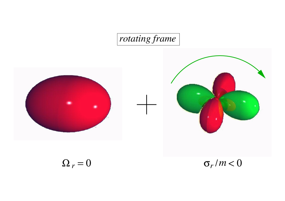
Figure 7: Schematic view from the rotating frame. The unperturbed star is shown on the left and the non-axisymmetric perturbation on the right. $\Omega_{r}=0$ and $\sigma_{r}/m$ are the angular velocities of the star and of the wave-pattern, respectively. Note that the star is effectively rotating as observed in an inertial frame and its structure, therefore, is deformed into a spheroid by the centrifugal stresses.

I will first discuss what would be observed in the rotating frame; this is summarized in Fig. 7 where I have shown schematically the unperturbed star on the left and the non-axisymmetric $l=m=2$ perturbation on the right. In the corotating frame the star has a zero angular velocity (i.e. $\Omega_{r}=0$), but is nevertheless deformed into a spheroid by the centrifugal force. The perturbation on the other hand, has a nonzero frequency $\sigma_{r}$ and the corresponding $m=2$ wave-pattern is seen to rotate with angular frequency $\sigma_{r}/m$ which is, say, negative. By definition, such a mode is referred to as “retrograde” and because the perturbed star is rotating at an angular velocity smaller than the initial one, the mode has a negative angular momentum $J_{0}<0$ in the corotating frame.

The non-axisymmetric perturbation generates a time-variation of the stellar mass multipoles (and/or of the mass-current multipoles) and the gravitational waves that are produced in this way, carry positive amounts energy at infinity. The angular momentum carried at infinity $j_{\rm gw}$ , on the other hand, can either be positive or negative according to the sense in which the perturbation is seen to rotate in the inertial frame. I therefore need to consider how the perturbation is observed in the inertial frame which, I recall, is the frame in which quantities like the total amount of energy and angular momentum can be measured unambiguously.

The “view” from the inertial frame is summarised in Fig. 8 where, again, I have shown schematically the unperturbed star on the left and the non-axisymmetric perturbation on the right. An observer in this frame will then see the star rotating at a nonzero, say positive, angular velocity $\Omega_{i}>0$ and the non-axisymmetric perturbation with a wave pattern that is also rotating with angular velocity $\sigma_{i}/m$.

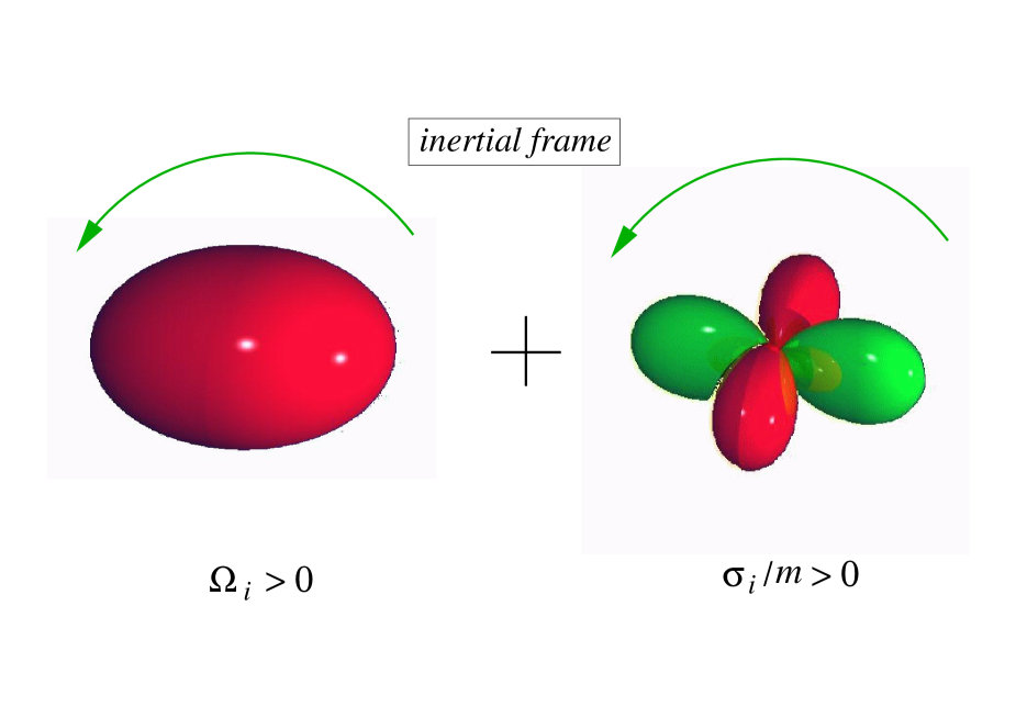
Figure 8: Schematic view from the inertial frame. The unperturbed star is shown on the left and the non-axisymmetric perturbation on the right. $\Omega_{i}$ and $\sigma_{i}/m$ are the angular velocities of the star and of the wave-pattern, respectively. Note that the star is seen to rotate and appears therefore as a spheroid.

It is not difficult to realize that the direction in which the wave-pattern rotates depends on both $\Omega_{i}$ and $\sigma_{r}$ through the relation between the frequencies in the two reference frames: $\sigma_{i}=m\Omega_{i}-\sigma_{r}$ [cf. expression (200)]. As a result, the wave-pattern can either be “dragged” forward ($\sigma_{i}>0>\sigma_{r}$), or backward ($\sigma_{i}<\sigma_{r}<0$) by the stellar rotation $\Omega_{i}$. The obviously interesting case shown in Fig. 8, is the one in which the mode is dragged forward (i.e. $\sigma_{i}/m>0$) and the non-axisymmetric mode, which is then said to be “prograde”, is seen to rotate in the same sense as the rotating star (Note that the “dragging” of the wave-pattern is a purely kinematical and Newtonian effect, fundamentally distinct from the general relativistic “dragging of reference frames”.). When this happens, $\Omega_{i}\sigma_{r}<0$ and the conditions for the onset of the CFS instability are met. In this case, in fact, and because the sign of the angular momentum lost is determined by the sense of rotation of the oscillation’s wave-pattern, the prograde non-axisymmetric perturbation will carry to infinity positive amounts of angular momentum, i.e. $j_{\rm gw}>0$.

For the observer in the rotating frame, on the other hand, the total angular momentum of the mode $J(t)\equiv J_{0}-j_{\rm gw}(t)$ becomes increasingly negative because of the losses through $j_{\rm gw}(t)$ that continuously reduce $J(t)$, i.e. $J(t)<J_{0}<0$. As a result, the initially small non-axisymmetric perturbation with negative angular momentum in the corotating frame, is driven to large amplitude oscillations with a progressively larger negative angular momentum. Such perturbation emits increasingly large amounts of gravitational waves, thus feeding the development of the instability. Using a pictorial analogue, the development of the CFS is similar to someone’s debts that get larger as new expenses (with positive amounts of money) are made. The growth of the instability stops when either nonlinear or dissipative effects become important and transfer energy from the unstable mode into the other available channels.

References

- [1] C. W. Misner, K. S. Thorne and J. A. Wheeler, “Gravitation”, Freeman, NY (1974)
- [2] B. F. Schutz, “An Introduction to General Relativity”, Cambrige Univ. Press, Cambridge UK (1984)
- [3] R. d’Inverno, “Introducing Einstein’s Relativity”, Oxford Univ. Press, Oxford UK (1990)
- [4] C. Cutler and K. S. Thorne, Proceedings of the GR16 Meeting, N. T. Bishop and S. D. Maharaj Eds., World Scientific (2002)
- [5] S. A. Hughes, Annals of Physics, in press, astro-ph/0210481 (2002)
- [6] T. Regge and J. A. Wheeler, Phys. Rev., 108 1063 (1957)
- [7] F. J. Zerilli, Phys. Rev. Letters, 24, 737 (1970)
- [8] C. V. Vishveshwara, Phys. Rev. D 1, 2870 (1970)
- [9] V. Moncrief, Annals of Physics, 88, 323 (1974)
- [10] K. S. Thorne, Rev. Mod. Phys., 52, 299 (1980)
- [11] S. Chandrasekhar, “The Mathematical Theory of Black Holes”, Oxford Univ. Press, Oxford UK (1992)
- [12] K. Kokkotas and B. Schmidt, Living Reviews, 2 (1999)
- [13] V. Ferrari, Review talk given at the EU Network Meeting, Thessaloniki (2001)
- [14] A. A. Starobinski and S. M. Churilov, Soviet JEPT, 38 (1973)
- [15] W. H. Press and S. A. Teukolsky, Astrophys. Journ., 185, 649 (1973)
- [16] J. A. Font, M. Miller, W. -M. Suen and M. Tobias, Phys. Rev. D 61, 044011 (2000)
- [17] M. Shibata and K. Uryu, Phys. Rev. D 61 06400 (2000)
- [18] J. A. Font, T. Goodale, S. Iyer, M. Miller, L. Rezzolla, E. Seidel, N. Stergioulas, W-M. Suen, and M. Tobias, Phys. Rev. D 65, 084024 (2002)
- [19] H. Dimmelmeier, J. A. Font and Ewald Müller, A&A 393 523; 388 917 (2002)
- [20] M. Shibata and K. Uryu, Prog. Theor. Phys., 107, 265 (2002)
- [21] M. D. Duez, P. Marronetti, S. L. Shapiro, T. W. Baumgarte, Phys. Rev. D, 024004 (2003)
- [22] B. F. Schutz Detection of gravitational waves in Proceedings of “Astrophysical sources of gravitational radiation”, J.A. Marck and J.P. Lasota Eds., Cambridge Univ. Press (1996)
- [23] R. C. Tolmann, Phys. Rev., 55, 364 (1939)
- [24] J. R. Oppenheimer and G. M. Volkoff, Phys. Rev., 55, 374 (1939)
- [25] J. M. Bardeen, K. S. Thorne and D. W. Meltzer, Astrophys. Journ., 145, 505 (1966)
- [26] E. N. Glass and L. Lindblom, Astrophys. Journ., 53, 93 (1983)
- [27] W. Unno, Y. Osaki, H. Ando, H. Saio and H. Shibahashi, Nonradial modes of oscillation, Tokyo Univ. Press (1989)
- [28] N. Stergioulas, Living Reviews, 8 (1998)
- [29] S. Chandrasekhar, “Stellar Structure”, Dover Pub., New York (1939)
- [30] J. L. Friedman and B. F. Schutz, Astrophys. Journ., 221, 937 (1978); 222, 281 (1978)
- [31] Tassoul, “Theory of Rotating Stars”, Princeton Univ. Press, Princeton (1978)
- [32] T. G. Cowling, Mon. Not. Roy. Astr. Soc., 101, 367 (1941)
- [33] J. R. Ipser and L. Lindblom, Astrophys. Journ., 389, 392 (1992)
- [34] S’i. Yoshida and Y. Eriguchi, Astrophys. Journ., 438, 830 (1995)
- [35] S’i. Yoshida and Y. Eriguchi, Astrophys. Journ., 490, 779 (1997)
- [36] H. Saio, Astrophys. Journ., 256 717, (1982)
- [37] N. Andersson and K. D. Kokkotas, Int. J. Mod. Phys. D 10, 381 (2001)
- [38] L. Rezzolla, F. K. Lamb, and S. L. Shapiro, Astroph. Journ. 531, L141-144 (2000)
- [39] L. Rezzolla, F. K. Lamb, D. Markovic, and S. L. Shapiro, Phys. Rev. D, 64, 104013 (2001); Phys. Rev. D, 64, 104014 (2001)
- [40] K. D. Kokkotas and B. F. Schutz, Mon. Not. Roy. Astr. Soc., 255 119 (1992)
- [41] S. Chandrasekhar, V. Ferrari, Proc. R. Soc. Lond. A 434, 635 (1991)
- [42] M. Leins, H.-P. Nollert, and M. H. Soffel, Phys. Rev. D, 48, 3467 (1993)
- [43] N. Andersson and K. D. Kokkotas, Mon. Not. Roy. Astr. Soc., 299, 1059 (1998)
- [44] N. Andersson, Y. Kojima and K. D. Kokkotas, Astrophys. Journ., 462 855 (1996)
- [45] S. L. Shapiro and S. A. Teukolsky, “Black Holes, White Dwarfs and Neutron Stars ”, J. Wiley NY (1984)
- [46] S. Chandrasekhar, Phys. Rev. Letters 24, 611 (1970)
- [47] N. Andersson, Clas. Quantum Grav. in press, (2002), astro-ph/0211057