Also at: ]Institute of Mathematics, Polish Academy of Sciences, Warsaw, Poland

Also at: ]Space Radiation Laboratory, California Institute of Technology, Pasadena, CA 91125

Resolving signals in the LISA data

Abstract

We estimate the upper frequency cutoff of the galactic white dwarf binaries gravitational wave background that will be observable by the LISA detector. This is done by including the modulation of the gravitational wave signal due the motion of the detector around the Sun. We find this frequency cutoff to be equal to $10^{-3.0}$Hz, a factor of 2 smaller than the values previously derived. This implies an increase in the number of resolvable signals in the LISA band by a factor of about 4.

Our theoretical derivation is complemented by a numerical simulation, which shows that by using the maximum likelihood estimation technique it is possible to accurately estimate the parameters of the resolvable signals and then remove them from the LISA data.

The gravitational waves from short-period binary systems containing white dwarfs and neutron stars are signals guaranteed to be observed by the Laser Interferometer Space Antenna (LISA) mission. Recent surveys indicate that there exist about twenty of such systems that are emitting gravitational radiation of frequency falling into the LISA band. Population studies have also shown that the number of such sources will be so large to produce a stochastic background that will lie significantly above the LISA instrumental noise in the low-part of its frequency band. It has been shown in the literature (see NYP00 for a recent study and HBW90 ; EIS87 for earlier investigations) that these sources will be dominated by detached white dwarf - white dwarf (wd-wd) binaries, with $1.1\ \times 10^{8}$ of such systems in our Galaxy. The detached wd-wd binaries evolve by gravitational-radiation reaction and the number of such sources rapidly decreases with increasing orbital frequency. It is therefore expected that above a certain limit frequency one will be able to resolve individual signals.

In this communication we calculate this limit frequency by including the effect of the signal modulation induced by the motion of LISA around the Sun. Earlier derivations assumed that one would be able to resolve only one signal per frequency bin. However, the modulation of the signal depends on the position of the source in the sky and therefore, by using matched-filtering technique, it is possible to resolve signals with same frequency but incoming from different directions.

The number distribution, $\frac{dN}{df}$, of the detached wd - wd binaries has been estimated in NYP00 to be equal to

$$\frac{dN}{df}=1\mbox{yr}\left(\frac{f}{f_{o}}\right)^{-\frac{11}{3}}\ ,$$ (1)

where yr is expressed in seconds, and $f_{o}=10^{-2.8}\$Hz. Thus, for an observation time of $n$ years, the number of sources in one frequency bin,$N_{s}$, can be approximated by the following formula

$$N_{s}=\left(\frac{f}{f_{o}}\right)^{-\frac{11}{3}}\frac{1}{n}.$$ (2)

If the signals were monochromatic one would expect to resolve roughly one source per frequency bin. Consequently, by equating $N_{s}$ to 1 and assuming 1 year of observation time, we would get an upper frequency cutoff equal to $f_{o}$. However, by accounting in the data analysis for the modulation of the signal due to the motion of LISA around the Sun, it is possible to resolve signals of equal frequency but incoming from different sky positions.

To estimate this effect we represent the LISA response, to a monochromatic gravitational wave signal, in the following form

$$h(t)=A_{o}\cos\Phi(t)\ ,$$ (3)

where the amplitude $A_{o}$ is assumed to be constant, and the phase $\Phi(t)$, which includes the Doppler modulation, is given by

$$\Phi(t)=\omega t+\frac{\omega R}{c}\cos(\lambda)\cos(\Omega t-\beta-\phi_{o})+\Phi_{o}.$$ (4)

Here $\omega$ is the angular frequency of the wave, $\Omega=2\pi/1$yr, ($\lambda,\beta$) are ecliptic coordinates of the source, $R=1$AU, $\phi_{o}$ is a known phase determining the position of the detector in the orbit around the Sun and $\Phi_{o}$ is an unknown, constant phase of the signal. This is a reasonable approximation since the time scale over which the detector’s response amplitude changes is significantly longer than that of the phase.

It is convenient to introduce the following linear parameterization of the signal

$$h(t)=A_{o}\cos[\Phi_{o}+\omega t+A\cos(\Omega t)+B\sin(\Omega t)],$$ (5)

where

$$A = \frac{\omega R}{c}\cos\lambda\cos(\beta-\phi_{o}),$$ (6)

$$B = \frac{\omega R}{c}\cos\lambda\sin(\beta-\phi_{o}).$$ (7)

In this parameterization the phase of the signal is a linear function of the signal’s unknown parameters ($\Phi_{0}$, $\omega$, A, B). The reduced normalized correlation function of the signal is given by JK00

$$C(\Delta w,\Delta A,\Delta B)= (\int^{1}_{0}\cos[\Delta wx+\Delta A\cos(2\pi nx)+\Delta B\sin(2\pi nx)]\,dx)^{2}+$$ (8)

$$(\int^{1}_{0}\sin[\Delta wx+\Delta A\cos(2\pi nx)+\Delta B\sin(2\pi nx)]\,dx)^{2},$$

where we have introduced a new dimensionless frequency parameter $w=1{\rm yr}\ n\ \omega$, and the new dimensionless time variable $x=t/({1{\rm yr}}\ n)$. The correlation function above is derived under the assumption that, over the bandwidth of the signal, the spectral density of the noise can be considered constant. As a consequence of the linearity of the phase of the signal in the parameters, the correlation function of two signals depends only on the difference between the values of the parameters and not on their absolute values. In the above parameterization the parameter space can be visualized as a truncated cone whose base and top are discs of radii $\frac{\omega_{u}R}{c}$ and $\frac{\omega_{l}R}{c}$ respectively, with $\omega_{u}$ and $\omega_{l}$ being the angular frequencies of the upper and the lower edge of the bandwidth of the detector. For a given angular frequency $\omega$ the parameter space is a disc of radius $\frac{\omega R}{c}$. Each point of the disc corresponds to two positions in the sky which differ by the sign in the ecliptic latitude angle $\lambda$.

In order to derive the background upper frequency cutoff we need to estimate the number of signals resolvable in a given frequency bin. This can be done by studying the correlation function between the signals in the A-B plane, and choosing a particular value for it. In this paper we have assumed two signals to be resolvable if their normalized correlation is less than 1/2. This choice of course is not optimal, and the final result of the upper frequency cutoff will depend on it. However, larger values of the correlation function imply a lower upper frequency cutoff, as it will be shown below. Here we do not identify the optimal value of the correlation function, which will be estimated in a forthcoming paper via Monte Carlo simulations. The reader should keep in mind this point when interpreting the conclusions of this paper.

The correlation surface in the A-B plane can be approximated by an ellipse whose area, $v_{AB}$, can be calculated using the covariance matrix (which is the inverse of the Fisher information matrix). The Fisher matrix, $\Gamma_{ij}$, for the signal (5) is given by

$$\Gamma_{ij}=\left(\begin{array}[]{cccc}1&\frac{1}{2}&\frac{\sin(2n\pi)}{2n\pi}&\frac{1-\cos(2n\pi)}{2n\pi}\\ \frac{1}{2}&\frac{1}{3}&-\frac{1-\cos(2n\pi)-2n\pi\sin(2n\pi)}{(2n\pi)^{2}}&\frac{\sin(2n\pi)-2n\pi\cos(2n\pi)}{(2n\pi)^{2}}\\ \frac{\sin(2n\pi)}{2n\pi}&-\frac{1-\cos(2n\pi)-2n\pi\sin(2n\pi)}{(2n\pi)^{2}}&\frac{4n\pi+\sin(4n\pi)}{8n\pi}&\frac{1-\cos(4n\pi)}{8n\pi}\\ \frac{1-\cos(2n\pi)}{2n\pi}&\frac{\sin(2n\pi)-2n\pi\cos(2n\pi)}{(2n\pi)^{2}}&\frac{1-\cos(4n\pi)}{8n\pi}&\frac{4n\pi-\sin(4n\pi)}{8n\pi}\\ \end{array}\right),$$ (9)

where $i,j=(\Phi_{o},w,A,B)$. Its expression has been derived under the assumption that, over the bandwidth of the signal, the spectral density of the noise can be considered constant. If we also assume the integration time to be a integer multiple of 1 year, then the Fisher matrix becomes

$$\Gamma_{ij}=\left(\begin{array}[]{cccc}1&1/2&0&0\\ 1/2&1/3&0&-1/(2n\pi)\\ 0&0&1/2&0\\ 0&-1/(2n\pi)&0&1/2\\ \end{array}\right)\ .$$ (10)

In the above expressions for $\Gamma_{ij}$ we have also normalized the signal-to-noise ratio to 1.

Since the area of the correlation ellipse is given by

$$v_{AB}=\frac{\pi\sqrt{det(C_{2})}}{2}=\frac{\pi^{2}n}{\sqrt{\pi^{2}n^{2}-6}},$$ (11)

where $C_{2}$ is the 2 by 2 sub-matrix of the covariance matrix for the parameters A and B, it follows that the number of resolved signals in a frequency bin centered on the frequency $f$ is given by the ratio of the area of the disc of radius $\frac{2\pi fR}{c}$, and the area of the correlation ellipse $v_{AB}$. In mathematical terms we have:

$$N_{r}=N_{o}\left(\frac{f}{f_{o}}\right)^{2},$$ (12)

with

$$N_{o}=\frac{\pi(2\pi f_{o}R/c)^{2}}{v_{AB}}.$$ (13)

If we equate the number of resolved signals, $N_{r}$, to the number $N_{s}$ of expected signals in one frequency bin (Eq. (2)), we get the following formula for the upper frequency cutoff, $f_{r}$, of the background

$$f_{r}=\frac{f_{o}}{(N_{o}n)^{3/17}}.$$ (14)

Equation (14) implies a frequency cutoff $f_{r}=10^{-3.0}\$Hz when a year of observation time is assumed.

By using the expression of the number of signals per frequency bin given in equation (1), we find that the number of detached white dwarf binaries above the frequency $f_{r}$ is around $6.8\ \times 10^{4}$. Although all these binaries can in principle be resolved, not all of them can be detected as some will have an amplitude smaller than the value of the detection threshold. To calculate the number of detectable binaries we first need to estimate the threshold corresponding to a satisfactory confidence of detection. We assume that we shall process the data by matched filtering. For the linear phase model of the signal given above we can adopt methods developed in JKS98 . First we need to calculate the number of cells, $N_{c}$, in the parameter space. These are the number of realizations of the optimal filter whose correlation is smaller than a pre-chosen value (1/2 in our case). This number is given by the ratio between the volume of the characteristic correlation hypersurface and the volume of the parameter space over which the search is performed. In our case the volume of the parameter space is given by

$$V=n\ {\rm yr}\ \frac{\pi}{3}\left(\frac{1\mbox{AU}}{c}\right)^{2}\ (\omega_{u}^{3}-\omega_{l}^{3})\ ,$$ (15)

while the volume $v$ of the correlation ellipsoid can be obtained by using the covariance matrix:

$$v=\frac{\pi\sqrt{2\ det(C_{3})}}{3}\ .$$ (16)

Here $C_{3}$ is the 3 by 3 sub-matrix of the covariance matrix for the parameters $w,A$, and $B$. In reference JKS98 , Eq.(77), it was shown that for Gaussian noise, the false alarm probability can be written as follows

$$P_{\rm F}=1-[1-e^{-{\cal F}_{0}}]^{N_{c}}\ ,$$ (17)

where ${\cal F}_{0}$ is the threshold on the following optimal statistics function JKS98

$${\cal F}=\frac{1}{n\ {\rm yr}\ S_{c}}\left|\int_{0}^{n{\rm yr}}\ y(t)\ e^{\ i\ [A\cos(\Omega t)+B\sin(\Omega t)+\omega t]}\ dt\right|^{2}.$$ (18)

In Eq. (18) $S_{c}$ is the value of the two-sided power spectral density of the noise estimated in the center of the frequency bandwidth of the signal, and $y(t)$ is the LISA data stream.

Equation (17) implies that, with a false alarm probability of $1$ percent, the corresponding threshold signal-to-noise ratio is equal to $7.6$. The corresponding number of resolvable white dwarf binaries with signal-to-noise above this threshold is equal to $3365$, under the assumption of sources uniformly distributed in the galactic disk. As a comparison, the number of resolvable binaries calculated without including the effects of the phase modulation of the signals is equal to 919, a factor of $3.7$ smaller than what we estimate.

This threshold is of course rather conservative, since it reflects the assumption that we are searching for one or more signals in the data, and we should therefore regard it as an upper-bound. In reality these signals are present in the LISA data and, in order to calculate the lower bound for the threshold, we can assume each cell to contain a signal. Consequently, the false-alarm probability becomes

$$P_{\rm F}=e^{-{\cal F}_{0}}\ ,$$ (19)

since now $N_{c}=1$ in equation (17). The corresponding threshold signal-to-noise ratio goes down to 2.7, again for a false alarm probability of $1$ percent. This implies that $47440$ white-dwarf binaries of signal-to-noise ratio larger than this threshold will be resolvable. If we neglect the effects of the phase modulation of the signals, the number of resolvable binaries is equal to $13178$ instead.

As a demonstration of how well the parameters of the signals can be estimated by using the maximum likelihood method, we have performed a numerical simulation of our technique. We first estimate the parameters of the strongest signal, we remove it from the data, and then iterate these two steps until no signal crosses our predefined threshold. The numerical procedure for locating the maximum consists of two steps. The first is a coarse search of the maximum of the likelihood function on a predefined grid in the parameter space. This is then followed by a refinement around the region of the parameter space where the maximum identified by the coarse search is located. This second stage of the maximization is performed by using a numerical implementation of the Nelder-Mead algorithm, where the starting point of the maximization is determined by the values of the parameters identified by the coarse search.

A graphical representation of the effectiveness of our method is presented in Figures 1 and 2, which correspond to two different combinations of signals in the LISA data. Both figures show two sinusoidal signals of identical frequencies, and incoming from different two directions in the sky. The correlation between the two signals was chosen to be approximately equal to 1/2. In figure 1 we input signals with signal-to-noise ratios equal to 7 and 20, while in Figure 2 the signal-to-noise ratios have been increased to 20 and 60 respectively. The common frequency of the signals ($f=1.5\ \times 10^{-3}$ Hz), and their incoming directions in the sky are unchanged in both figures.

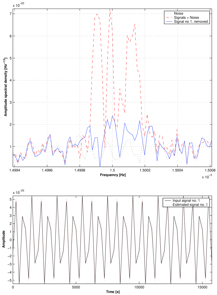
Figure 1: Estimation and removal of one of two signals from the LISA data stream using a two-step maximum likelihood estimation. The two signals have signal-to-noise ratios equal to 7 and 20 respectively, their frequencies are equal, but they originate from different points in the sky. The upper part of the figure shows the power spectra of the signals and the noise (dashed line), of the data after the stronger signal is removed (solid line), and of the noise only (dotted line). The lower part instead compares the shape of the signal injected (solid line) into the LISA data against that of the estimated one (dotted line).

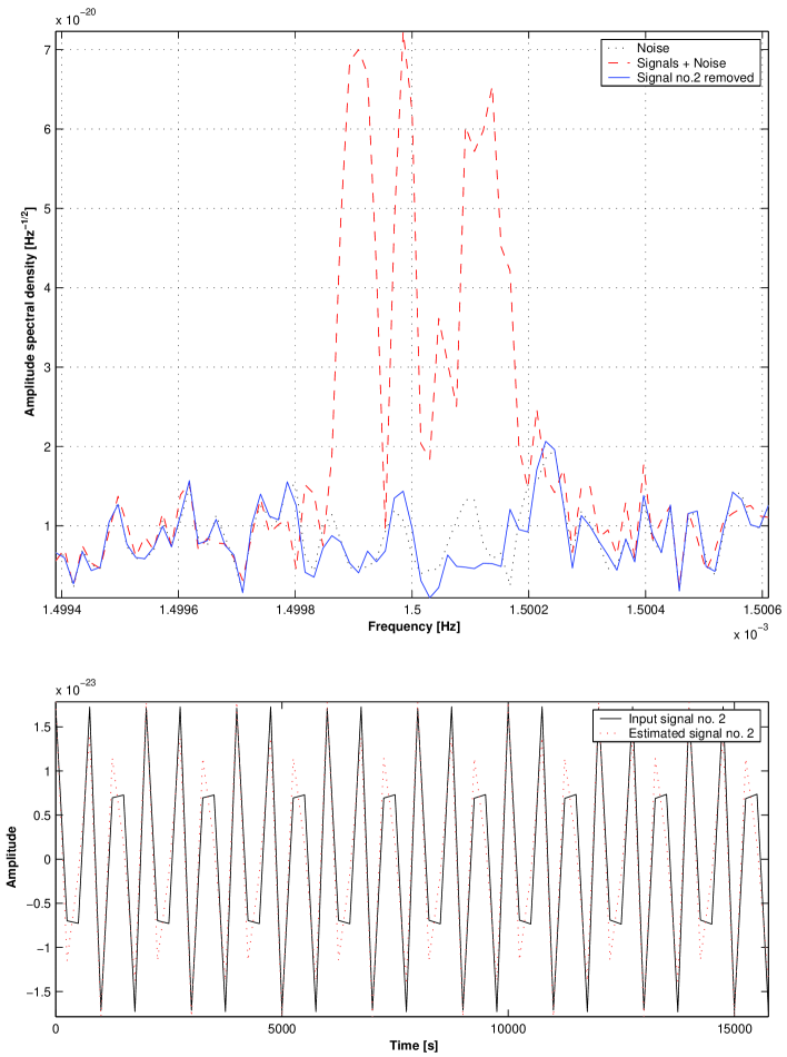
Figure 2: The signals are as in Figure 1a, but now the spectra shown include one in which the signals are both removed (solid line).

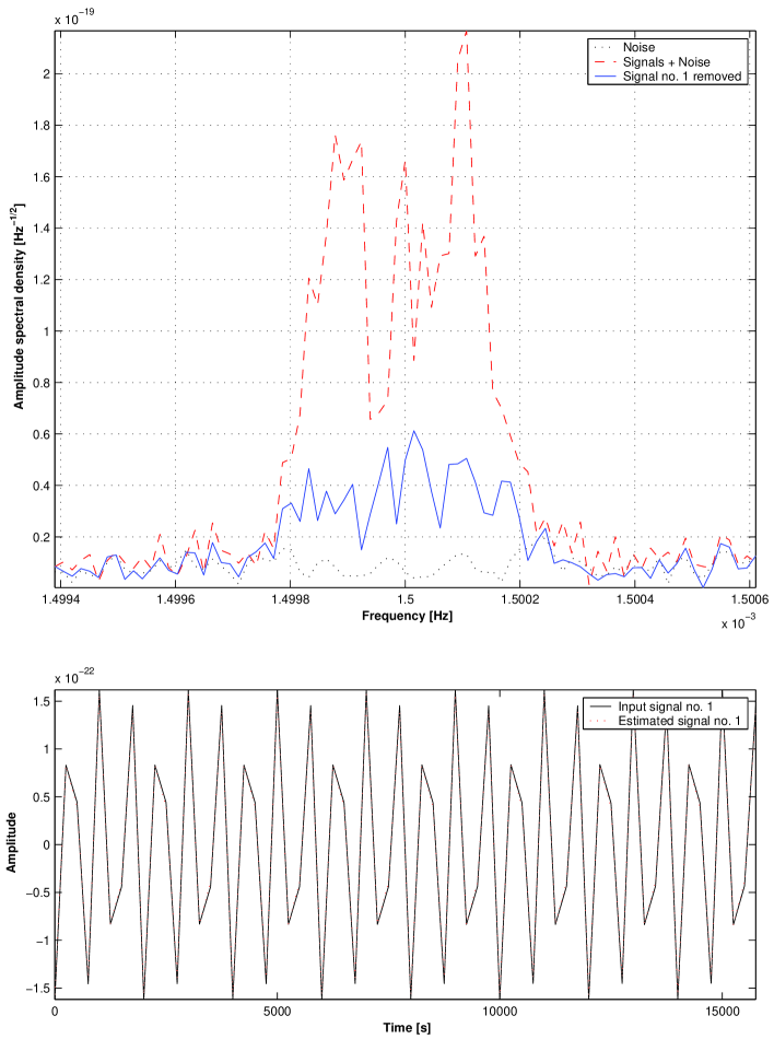
Figure 3: As Figure 1a, but now the signal-to-noise ratios have been increased to 20 and 60 respectively

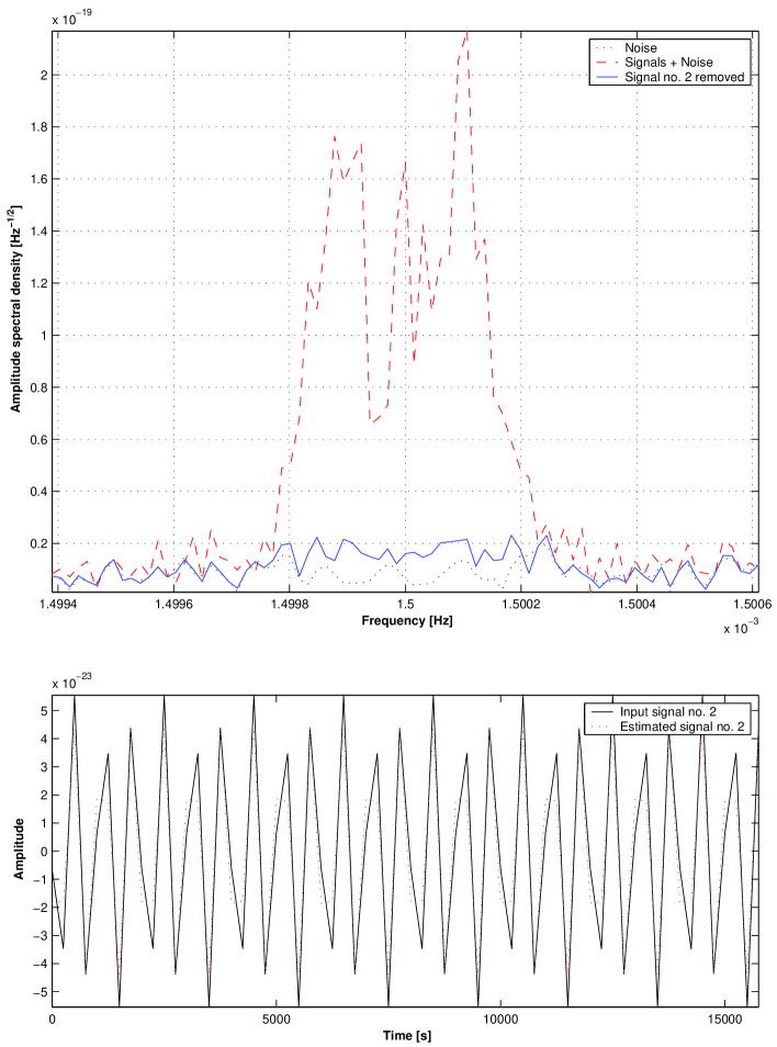
Figure 4: The same as Figures 1b, but the signals have signal-to-noise ratios equal to 20 and 60

A visual inspection of the plots shows that the estimation of the parameters and the resolution of the signals (with the use of the maximum likelihood method) can be expected to be satisfactory for removing them from the data. This will make possible the search of other signals potentially present in the LISA data.

References

- (1) G. Nelemans, L. R. Yungelson, and S. F. Portegies-Zwart, A&A 375, 890 (2001).
- (2) D. Hils, P. L. Bender, and R. F. Webbink, ApJ 360, 75 (1900).
- (3) Ch. Evans, Ickp Iben, and L. Smarr, ApJ 323, 129 (1987).
- (4) P. Jaranowski, A. Królak, and B. F. Schutz, Phys. Rev. D 58, 063001 (1998).
- (5) P. Jaranowski and A. Królak, Phys. Rev. D 61, 062001 (2000).