Adaptive Mesh Refinement for Characteristic Codes

Abstract

The use of adaptive mesh refinement (AMR) techniques is crucial for accurate and efficient simulation of higher dimensional spacetimes. In this work we develop an adaptive algorithm tailored to the integration of finite difference discretizations of wave-like equations using characteristic coordinates. We demonstrate the algorithm by constructing a code implementing the Einstein-Klein-Gordon system of equations in spherical symmetry. We discuss how the algorithm can trivially be generalized to higher dimensional systems, and suggest a method that can be used to parallelize a characteristic code.

1 Introduction

The investigation of the characteristic structure of a system of partial differential equations (PDEs) gives valuable insight on the behavior of allowed solutions. Analytical studies have long benefited from understanding and employing this knowledge. In the numerical realm, efficient algorithms have been developed which exploit the underlying characteristic structure. These algorithms are obtained by formally transforming to characteristic variables, realizing how these need to be updated, and then employing this information to construct an algorithm using the original variables. However, the explicit integration along characteristics, where coordinates are chosen adapted to the characteristic directions, has received considerably less attention. Indeed, this option has so far only been actively pursued within general relativity (GR), although as discussed in[1, 2] there are powerful reasons to consider this option in systems described by wave-like equations.

The characteristic formulation of general relativity has since its introduction in the 60’s played an important role as a tool to investigate different aspects of the theory (see for instance [3, 4, 5, 6, 7, 8].) A clean picture of the effect of gravitational waves and their geometric manifestation, links between the structure of future null infinity and some interior sources, and the analysis of singularity structure are some areas that have effectively been tackled by this approach.

In recent years, the formalism has also displayed its usefulness in the numerical arena. Investigations of critical phenomena[9, 10, 11, 12, 13], wave propagation on non-trivial backgrounds[14] and simulations of spacetimes containing black holes[15, 16, 17, 18] or neutron stars[19] have benefited from exploiting this approach. Numerical simulations of black hole spacetimes are of considerable importance for the detection and analysis of gravitational waves that could be measured by the new generation of gravitational wave detectors. Among the systems expected to produce gravitational waves of sufficient intensity are those containing black holes and neutron stars, and it would be ideal if the success obtained simulating single black holes with 3D characteristic codes could be translated to these systems. Preliminary indications that this is likely the case for a subset of possible black hole-neutron star binaries can be found in [20, 19], where higher dimensional, non-vacuum scenarios (yet simpler than the 3D binary black hole-neutron star system) have been accurately simulated.

Unfortunately, the computational requirements for modeling a binary black hole-neutron star system are quite high if one of the goals is to predict the waveforms produced by it in a quantitative manner. Since the expected energy output in gravitational waves is at most a few percent of the total mass of the system, the numerical simulation must guarantee that any systematic (numerical) error is well below this target. The major issue in achieving an accurate description of the system, when a stable discretization has been obtained, is to adequately resolve the different length scales involved. These scales are naturally defined by the stellar dynamics, the black hole, and the distant weak-field regime where the gravitational waves are extracted. Covering all of these scales with a uniform grid (in a finite-difference based numerical simulation) of sufficient resolution to accurately model the smallest features is not only a waste of resources, but may be impossible to achieve on contemporary computers. Therefore, we need to use techniques that better exploit available resources. One such technique is adaptive mesh refinement (AMR), whereby the simulation can dynamically adjust the grid resolution in different regions of the domain to adequately resolve all features with sufficient, but not excess, resolution.

In this paper we investigate the use of AMR techniques for characteristic evolution. Although we concentrate on the GR case, the algorithms presented here can readily be applied to many other equations. The use of characteristic AMR in GR has been partially addressed by several authors in the past[9, 10, 12], however, in those cases the algorithms were geared to studying gravitational collapse and singularity structure in spherical symmetry, and the techniques do not generalize to higher dimensional systems. Here we present an AMR algorithm for characteristic evolution that can be applied to scenarios with an arbitrary number of non-trivial spatial dimensions. Furthermore, the algorithm does not place significant restrictions on the discretization scheme, and hence existing unigrid codes (as described, for instance, in [21, 15, 22, 23, 17, 18]) can, in principle, be incorporated into the adaptive framework in a straight-forward manner. To demonstrate the basic algorithm, and show that it can adapt to dynamical features of a solution, we have implemented a spherically symmetric code to solve the Einstein-Klein-Gordon system.

The rest of the paper is organized as follows. In Sec. 2 we describe the coordinate system, set of equations and corresponding discretization scheme that we will employ in the example problem. We use a coordinate system with a single null direction, however, the AMR algorithm is most easily presented for double null coordinates; hence in Sec. 3 we describe the adaptive scheme for double null evolution. In section 4 we mention how the basic algorithm is extended to a coordinate system with a single null coordinate, how additional non-trivial spacelike dimensions can be handled, mention some problem specific features such as the numerical dissipation and interpolation operators we use, and describe a method that can be used to parallelize a characteristic code (with or without AMR). In Sec. 5 we present results from our spherically symmetric code, and give some concluding remarks in Sec. 6.

2 The spherically symmetric Einstein-Klein-Gordon problem in the characteristic approach

Einstein’s equations can be expressed in notational form as $G_{ab}=8\pi T_{ab}$, where $G_{ab}$ is the Einstein tensor and $T_{ab}$ the stress energy tensor of the matter distribution. In the particular case of a scalar field $\Phi$ coupled to GR, $T_{ab}$ results in[24]

$$T_{ab}=\nabla_{a}\Phi\nabla_{b}\Phi-1/2\,g_{ab}\left(\nabla_{c}\Phi\nabla^{c}\Phi+m^{2}\Phi^{2}\right)\,$$ (1)

where $g_{ab}$ is the metric tensor, and $m$ is the mass parameter of the scalar field.

We introduce a coordinate system adapted to incoming null hypersurfaces in the following way: incoming lightlike hypersurfaces are labeled with a parameter $v$, each null ray on a specific hypersurface is labeled with $(\theta,\phi)$ and $r$ is introduced as a surface area coordinate (i.e. surfaces at $r={\rm const.}$ have area $4\pi r^{2}$). In these coordinates, the metric takes the Bondi-Sachs form[3, 4]

$$ds^{2} = e^{2\beta}V/rdv^{2}+2e^{2\beta}dvdr+r^{2}d\Omega^{2},$$ (2)

Note that the choice of incoming null surfaces is merely for convenience; the trivial change $\beta\rightarrow\beta+i\pi$ takes the line element (2) into the one corresponding to outgoing null surfaces (further details can be found in [25]). The algorithm presented here can easily be modified to handle the outgoing case.

In order to express the equations of motion in a simpler form, we introduce the following variables

$$V \equiv -r+g$$ (3)

$$\Psi = r\Phi\,.$$ (4)

The resulting equations (provided by $R_{rr}=8\pi\Phi_{,r}^{2}$, $R_{\theta\theta}=8\pi\Phi_{,\theta}^{2}$ and $\Box\Phi=0$ respectively, where $R_{ab}$ is the Ricci tensor) reduce to:

$$\beta_{,r} = 2\pi\,\frac{(r\Psi_{,r}-\Psi)^{2}}{r^{3}}\,,$$ (5)

$$g_{,r} = 1-e^{2\beta}\left(1-4\pi m^{2}\Psi^{2}\right)\,,$$ (6)

$$2(\Psi)_{,rv} = -\left(1-\frac{g}{r}\right)\Psi_{,rr}+\left(\frac{g}{r}\right)_{,r}\left(\Psi_{,r}-\frac{\Psi}{r}\right)+e^{2\beta}m^{2}\Psi$$ (7)

A properly posed problem requires data to be given on an initial $v=v_{o}$ hypersurface (which consists only of the unconstrained $\Psi$) and consistent boundary data on an intersecting surface (which includes $\Psi$, $g$ and $\beta$). The boundary data comprises gauge, physical and constrained data. For instance, given the value of $\beta$ and $\Psi$ on an $r={\rm const.}$ surface the value of $g$ is determined by the remaining Einstein equation $R_{vv}=8\pi\Phi_{,v}^{2}$ (which we call the consistency equation). Next we describe the particular setting used in the tests performed throughout this work.

2.1 Coordinate conditions and boundary data

For our present purposes we choose the outer boundary to coincide with past null infinity (${I}^{-}$). At ${I}^{-}$ we fix a Bondi coordinate system, therefore $\beta=0$ (i.e. $v$ represents the affine time of observers at ${I}^{-}$). Since past infinity is a null hypersurface, data for $\Psi$ is unconstrained and in fact is intimately related (just a time derivative difference) to the “Bondi News” which is the incoming radiation from past null infinity. We provide data for $\Psi$ arbitrarily, and then determine the value of $g$ using the consistency equation, which on ${I}^{-}$ reduces to:

$$g_{,v}=8\pi(\Psi_{,v})^{2}\,.$$ (8)

2.2 Numerical Implementation

We discretize equations (5,6,7,8) using second order finite difference (FD) techniques. In order to include ${I}^{-}$ in our computational grid, we introduce a compactified radial coordinate $x=r/(1+r)$ (hence $r\in[0,\infty)$) [23] . This coordinate is uniform in the domain $[0,1]$ and is discretized by $x_{i}=(i-1)\Delta x$, with $i=1,2,...,N_{x}$; similarly, $v$ is discretized so that $v^{n}=(n-1)\Delta v$, with $n=1,2,...,N_{v}$. As is customary, we label a grid function $f$ at coordinate location ($x_{i},v^{n}$) by $f^{n}_{i}$—see Fig. 1 below for a schematic representation of the coordinate system and discretization. The boundary data is specified along the pair of intersecting null surfaces $x=1$ (${I}^{-}$) and $v=0$. Integration of the evolution and hypersurface equations (5-7) then proceeds via a sequence of radial integrations (inwards, from $x=1-\Delta x$ to $x=0$) along each of the null surfaces from $v=\Delta v$ to $v=V_{1}$. Specifically, the discretized hypersurface equations read:

$$\beta^{n+1}_{i} = \beta^{n+1}_{i+1}-2\,\pi\,\Delta x\,\frac{(1-x_{c})}{x_{c}^{3}}\,\left(x_{c}(1-x_{c})\Psi_{,x}|_{o}-\Psi|_{o}\right)^{2}\,,$$ (9)

$$g^{n+1}_{i} = g^{n+1}_{i+1}-\Delta x\,(1-x_{c})^{2}\,(1-e^{2\beta|_{o}}(1-4\pi m^{2}\Psi|_{o}^{2}))\,\,,$$ (10)

where

$$x_{c} = (x_{i}+x_{i+1})/2\,,$$ (11)

$$\Psi|_{o} = (\Psi^{n+1}_{i}+\Psi^{n+1}_{i+1})/2\,,$$ (12)

$$\Psi{,x}|_{o} = (\Psi^{n+1}_{i+1}-\Psi^{n+1}_{i})/\Delta x\,;$$ (13)

and similarly for $\beta|_{o}$. The evolution equation for $\Psi$ is evaluated at the point $(v^{n}+\Delta v/2,x_{i}+\Delta x/2)$ by including the points $(v^{n+1},x_{i})$, $(v^{n+1},x_{i+1})$, $(v^{n+1},x_{i+2})$, $(v^{n},x_{i-1})$,$(v^{n},x_{i})$ and $(v^{n},x_{i+1})$:

$$\Psi^{n+1}_{i} = -\Big{(}-\Psi^{n+1}_{i+1}\,\left(x_{c}+\frac{\Delta v}{2\Delta x}(1-x_{c})^{2}F_{1}\right)$$ (14)

$$+\Psi^{n+1}_{i+2}\,\left(\frac{\Delta v}{4\Delta x}(1-x_{c})^{2}F_{1}\right)+x_{c}(\Psi^{n}_{i+1}-\Psi^{n}_{i})$$

$$+\frac{\Delta v}{4\Delta x}(1-x_{c})^{2}F_{1}(\Psi^{n}_{i+1}-2\Psi^{n}_{i}+\Psi^{n}_{i-1})$$

$$-F_{1}\Delta x\Delta v\Psi_{,x}|_{c}(1-x_{c})$$

$$+\frac{\Delta v\Delta x}{2}(1-x_{c})\left((1-x_{c})g_{,x}|_{c}-\frac{g|_{c}}{x_{c}}\right)\,\left((1-x_{c})\Psi_{,x}|_{c}-\frac{\Psi|_{c}}{x_{c}}\right)$$

$$+\frac{x_{c}\Delta x\Delta v}{2(1-x_{c})^{2}}e^{2\beta|_{c}}m^{2}\Psi|_{c}\Big{)}$$

$$/\left(x_{c}+\frac{\Delta v}{4\Delta x}(1-x_{c})^{2}F_{1}\right)$$

where

$$g|_{c} = (g^{n}_{i}+g^{n+1}_{i+1})/2$$ (15)

$$g_{,x}|_{c} = (g^{n+1}_{i+2}-g^{n+1}_{i+1}+g^{n}_{i}-g^{n}_{i-1})/2/\Delta x$$ (16)

$$F_{1} = -x_{c}+g|_{c}(1-x_{c})\,,$$ (17)

and analogously for $\Psi_{c}$, $\beta|_{c}$ and $\Psi_{,x}|_{c}$. For each integration step (14) is first used to solve for $\psi^{n+1}_{i}$, then (9) is solved for $\beta^{n+1}_{i}$, and finally we obtain $g^{n+1}_{i}$ from (10). Note that at the first radial point in from ${I}^{-}$ (at $x=1-\Delta x$) there are insufficient points available to evaluate $g_{,x}|_{c}$ via the above scheme, and so there we simply propagate $\Psi$ inwards using

$$\Psi^{n+1}_{N_{x}-1}=\Psi^{n+1}_{N_{x}}.$$ (18)

\psfrag{A}{$f^{n+1}_{i}$}\psfrag{B}{$f^{n}_{i}$}\psfrag{C}{$f^{n}_{i+1}$}\psfrag{D}{$f^{n+1}_{i+1}$}\psfrag{E}{$f^{n}_{i-1}$}\psfrag{F}{$f^{n+1}_{i+2}$}\psfrag{x}{$x$}\psfrag{v}{$v$}\psfrag{x0}{$(0,0)$}\psfrag{v1}{$(1,V_{1})$}\psfrag{xv0}{$(x,v)=(1,0)$}\includegraphics[width=341.43306pt,clip={true}]{bblock_xv_new.eps}

Figure 1: A schematic representation of the $(x,v)$ coordinate system (2) and discretization scheme on a spactime diagram, where null directions are at 45 degree angles relative to the vertical, and timelike (spacelike) curves have tangent vectors less than (greater than) 45 degrees. The coordinate lines $v={\rm const.}$ are ingoing null curves, and $x={\rm const.}$ ($<1$) are timelike curves of constant areal radius. For reference, outgoing null curves (thinner dotted lines) are also shown on the plot. Note that $x={\rm const.}$ becomes null in the limit $x\rightarrow 1$, corresponding to past null infinity. The discretization of a variable $f$ is also shown on the figure—the points labelled correspond to those that need to be provided (in general) as “initial data” to solve for the unknown $f_{i}^{n+1}$ at the interior point ($x_{i},v^{n+1}$).

Regularity conditions at $x=0$ are explicitly enforced for $\Psi$ $\{\Psi(x=0,v)=0\}$ and $\beta$ $\{\beta_{x}(x=0,v)=0\}$. Furthermore we set $\Psi(x=\Delta x,v)$ using fourth order interpolation:

$$\Psi^{n+1}_{1} = 0,$$ (19)

$$\Psi^{n+1}_{2} = 3\Psi^{n+1}_{3}/2-\Psi^{n+1}_{4}+\Psi^{n+1}_{5}/4,$$ (20)

$$\beta^{n+1}_{1} = 4\beta^{n+1}_{2}/3-\beta^{n+1}_{3}/3.$$ (21)

On the outgoing ($x=1$) and ingoing ($v=0$) initial characteristics, we freely specify $\Psi$. We set $g(x=1,v=0)=2m_{0}$, where $m_{0}$ is the initial, asymptotic mass of the spacetime. We then integrate (9-10) to obtain $\beta(x,v=0)$ and $g(x,v=0)$, and integrate (8) along $x=1$ (using a similar discretization to (10)) to obtain $g(x=1,v)$.

We employ black hole excision techniques to solve for spacetimes containing a black hole, and consequently a geometric singularity. Here the underlying assumption is that cosmic censorship holds: any singularity will be hidden by an event horizon (black hole), and hence cannot causally influence the region outside the black hole[26]. This feature is exploited by placing an inner boundary inside the event horizon, preventing the simulation from getting too close to the singularity. One cannot determine the location of the event horizon prior to solving for the geometry of the entire spacetime; however, we can use the location of an apparent horizon to tell us where to excise, for under reasonable assumptions the apparent horizon always lies inside the event horizon[27]. An apparent horizon is defined as the outermost, closed surface whose outgoing null rays form a non-divergent front (i.e the surface is ‘trapped’). The location of the apparent horizon is given by $V=0$ in (2). In practice, when we detect an apparent horizon, we excise the portion of the grid interior to it, though we leave a small buffer zone between the apparent horizon and actual excision surface (which is inside the apparent horizon). We implement excision by extrapolating all variables, using fourth order extrapolation, to all points interior to the surface of excision. Thus the “solution” we obtain inside the black hole is not physically meaningful, but the excision does not adversely affect the exterior part of the solution that we are interested in.

3 AMR in double null coordinates

Here we motivate and describe our AMR algorithm for characteristic codes. The salient features of the algorithm are best demonstrated in a double null coordinate system; therefore we first describe the algorithm in detail for this case, and then discuss the modifications for the spacelike-null situation in the following section.

Our AMR algorithm is modeled after the Berger and Oliger (B&O) algorithm [28] for hyperbolic, Cauchy problems. The B&O algorithm has several desirable features that we have used as cornerstones in building the scheme for characteristic codes:

• the computational domain is decomposed into a grid hierarchy, whereby the partial differential equations are discretized using identical unigrid finite difference schemes on each grid within the hierarchy.

• dynamical regridding is performed via local truncation error (TE) estimates.

• the recursive evolution algorithm makes efficient use of resources in both space and time, for the grids are always evolved with a time step set by the local spatial discretization scale (to satisfy the CFL condition), and not by the smallest scale within the problem.

It is not possible to directly apply the B&O algorithm in a double null coordinate system by (for instance) treating one of the null coordinates as the “spatial” coordinate and the other as “time”, and then integrating the “spatial” surfaces in “time”. This is because propagation along the null surface masquerading as a spatial surface will be instantaneous, and hence the local TE estimation scheme will not be able to track corresponding features of the solution. The key to adapting B&O to characteristic codes is to effectively consider each null direction as “time”, and then to simultaneously evolve along both.

In the double null evolution algorithm the structure of the grid hierarchy goes hand-in-hand with the evolution scheme, so we first describe the hierarchy in detail before presenting the evolution scheme.

3.1 AMR grid hierarchy

For the following discussion we will consider the discretization of a double null coordinate system $(u,v)$, where $u={\rm const.}$ labels an outgoing null curve, and $v={\rm const.}$ an ingoing null curve. For example, a coordinate transformation of the form $du=-e^{2\alpha}\left(Vdv/r+2dr\right)$, with $e^{2\alpha(v,r)}$ an integrating factor, will bring (2) into the form

$$ds^{2}=-e^{2\xi}dudv+r^{2}d\Omega^{2},$$ (22)

where $\xi$ and $r$ are now considered functions of $u$ and $v$.

The AMR grid hierarchy (see Fig. 2 below for an example) consists of a sequence of $N$ levels: $\ell_{1},\ell_{2},...,\ell_{N}$, where all grids at level $m$ are discretized on a uniform mesh with $[\Delta u_{m},\Delta v_{m}]=[\Delta u_{1}/\rho^{m-1},\Delta v_{1}/\rho^{m-1}]$, and $\rho$ is the refinement ratio. Therefore, higher levels (larger level numbers) are composed of finer grids. In this paper we only consider $\rho=2$, however the generalization to arbitrary integer values of $\rho\geq 2$ is straight-forward (as is the generalization to different refinement ratios for each level). All grids at level $m$ are entirely contained within grids at level $m-1$. What we mean by this is that the coordinate region spanned by the union of grids at level $m$ is a subset of the coordinate region of the union of grids at level $m-1$. Furthermore, we require that the meshes of all levels be aligned such that any point $(u^{i},v^{j})$ in a grid at level $m-1$ within the region of overlap between levels $m$ and $m-1$ (a parent point) be coincident with a point on a grid at level $m$ (a child point). This alignment of grids between levels is essential for the recursive evolution algorithm (and useful for truncation error estimation), as will be explained in the next section. As an aside, note that the characteristic AMR algorithm could still allow for rotation of child grids in higher dimensional ($>2$) simulations in the same sense as the original B&O algorithm, however, here the rotation would be within a subspace orthogonal to $u={\rm const.},v={\rm const.}$. In other words, we only require rigid alignment of the two “time” coordinates $u$ and $v$.

\psfrag{cgs}{\Large Composite Grid Structure}\psfrag{du1}{$\Delta u_{1}$}\psfrag{du2}{$\Delta u_{2}$}\psfrag{du3}{$\Delta u_{3}$}\psfrag{du4}{$\Delta u_{4}$}\psfrag{dv1}{$\Delta v_{1}$}\psfrag{dv2}{$\Delta v_{2}$}\psfrag{dv3}{$\Delta v_{3}$}\psfrag{dv4}{$\Delta v_{4}$}\psfrag{u}{\Large$u$}\psfrag{v}{\Large$v$}\psfrag{l1}{\Large Level 1}\psfrag{l2}{\Large Level 2}\psfrag{l3}{\Large Level 3}\psfrag{l4}{\Large Level 4}\includegraphics[width=398.33858pt,clip={true}]{sample_mesh.eps}

Figure 2: An example of a double null grid hierarchy. The upper-most figure shows the entire hierarchy, composed of four levels in this case. Each level is stored independently of the others; in the lower plots we show the structure of each of these levels.

3.2 Evolution Scheme

Evolution of PDEs discretized on the kind of grid hierarchy just described proceeds by recursively evolving a particular sequence of unigrid unit cells, from the coarsest to finest levels, and then propagating the solution obtained on the finer levels back to the coarser ones. The unit cell for a typical double null discretization scheme is shown in Fig. 3. For a concrete example, consider the spherically symmetric wave equation on a flat background (whose line element is $ds^{2}=-dudv+r^{2}d\Omega^{2}$, where $r=(v-u)/2$):

$$\Box{\phi}=0\rightarrow\phi_{,uv}+\frac{1}{2r}\left(\phi_{,u}-\phi_{,v}\right)=0$$ (23)

A second order accurate finite difference version of (23), discretized on the unit cell of Fig. 3, is[29]

$$\frac{\phi_{A}+\phi_{C}-\phi_{B}-\phi_{D}}{\Delta u\Delta v}+$$

$$\frac{1}{2r}\left(\frac{\phi_{A}+\phi_{B}-\phi_{C}-\phi_{D}}{2\Delta u}-\frac{\phi_{A}+\phi_{D}-\phi_{B}-\phi_{C}}{2\Delta v}\right) = 0.$$ (24)

Initial data for $\phi$ must be specified on the initial ingoing and outgoing characteristics, which amounts to specifying $\phi$ at points $B,C$ and $D$. Evolution to point $A$ then proceeds by solving (3.2) for $\phi_{A}$. Evolution of $\phi$ over an entire uniform mesh of cells is then trivial (ignoring boundary conditions)—the unit cell evolution scheme is repeatedly applied, in arbitrary order, to all cells where past values (corresponding to points $A,C$ and $D$) of $\phi$ are known, until all points in the grid are solved for.

\psfrag{A}{$A$}\psfrag{B}{$B$}\psfrag{C}{$C$}\psfrag{D}{$D$}\psfrag{n}{$n$}\psfrag{s}{$s$}\psfrag{e}{$e$}\psfrag{w}{$w$}\includegraphics[width=227.62204pt,clip={true}]{bblock.eps}

Figure 3: A fundamental unit cell of the double null evolution scheme. The unit cell consists of the four points $A,B,C$ and $D$. In the plot we also schematically show part of the data structure we use to represent the hierarchy, namely, a set of point-structures (or points for short), linked together to form the mesh. Each point contains north ($n$), south ($s$), east ($e$) and west ($w$) links to adjacent points at the same level, as shown for point $C$. In addition, certain points will have parent and/or child links to corresponding points in the parent and/or child levels (not shown in the figure).

The extension of this unigrid evolution scheme to an adaptive hierarchy is for the most part straightforward, and follows the B&O scheme rather closely in spirit. The evolution algorithm consists of a particular sequence of single, unit cell evolution steps. The order in which cells are traversed over the hierarchy is dictated by causality, in that we can only evolve to point $A$ if the “initial/boundary data” at points $B,C$ and $D$ are known. However, notice in Fig. 2 (and below in the first frame of Fig. 5, depicting a sample evolution) that this initial data will not be available on a finer level $m>1$ with initial surfaces $u=U_{m}$ or $v=V_{m}$ that are interior to the computational domain boundaries, i.e. where $U_{m}>U_{1}$ or $V_{m}>V_{1}$ (we assume that at $u=U_{1}$ and $v=V_{1}$ the entire initial grid structure is supplied—see Sec. 4 for a discussion on how the initial hierarchy could be calculated). The solution to this problem is to always evolve coarser, parent cells first, and use the solution obtained on a parent cell to set initial data, via interpolation, at child cell points bounding a newly refined region. Then, evolution on the set of child cells is performed, recursively evolving additional finer levels if present. The solution obtained at points coincident with points on the parent level are injected back to the parent level, to maintain a single-valued solution where the most accurately known values are stored at all points in the hierarchy.

In theory, using interpolation to set interior initial data of fine regions will not adversely affect the consistency of the FD approximation to the PDEs if the hierarchy is generated via local truncation error (TE) estimates . For then, prior to the surface $u=U_{\ell}$ (or $v=V_{\ell}$) when a new fine level $\ell$ is added, the local TE on level $\ell-1$ will have the same order of magnitude as the maximum allowed TE, and hence if a sufficiently high order of interpolation is used to initialize the fields at $u=U_{\ell}$ ($v=V_{\ell}$) the solution error on level $\ell$ will differ from that on level $\ell-1$ by an amount less that the local TE there. In practice, interpolation often introduces high frequency solution components (“noise”) that produce a significant amount of error when propagated away from the refinement boundaries during subsequent evolution. Adding numerical dissipation to the FD scheme can significantly reduce this noise, as can the choice of interpolation operator and the frequency of regridding. These issues will be discussed in more detail later on in this section, and in Sec. 4.1.1.

The rule that we always evolve a parent cell before any child cells is naturally implemented via a recursive subroutine, which is summarized in pseudo-code in Fig. 4 below. The steps taken in a sample, 3-level evolution is depicted in Fig. 5. One of the differences of the characteristic AMR algorithm, compared to the B&O algorithm, is that a slightly more complicated data structure is needed to efficiently represent the dynamical hierarchy. In B&O, the grid hierarchy is calculated over the entire spatial hypersurface at a given time, and hence the grids at a given level can efficiently be stored as a list of one dimensional arrays (in a 1+1 D simulation). In the characteristic algorithm, the structure of the hierarchy is revealed point-by-point, simultaneously in the $u$ and $v$ directions as one evolves, and hence one cannot pre-allocate similar one dimensional arrays. We have chosen to use a data structure where a point $(u^{i},v^{j})$, at some level $\ell$, is the fundamental unit of data. The mesh is then constructed by linking together adjacent points at the same level with north($n$), south($s$), east($e$) and west($w$) pointers as depicted in Fig. 3, and linking points at the same coordinate location in levels $\ell-1$ and $\ell+1$ via parent and child pointers respectively. In the pseudo-code in Fig. 4 we have used C programming language notation to represent links; for example, referring to Fig. 3, ${\rm A=B\rightarrow n}$, and ${\rm B=A\rightarrow s}$. In the following paragraphs we will discuss key lines of the pseudo-code in detail.

 1:   logical function evolve_unit_cell(point C)
 2:      if (can_take_step(C)==false) then
 3:         return(false);
 4:      end if
 5:
 6:      if (point B=C->w does not exist) then
 7:         create B and link it into the surrounding mesh;
 8:         initialize variables at B via interpolation from parent points;
 9:      end if
10:      if (point D=C->n does not exist) then
11:         create D and link it into the surrounding mesh;
12:         initialize variables at D via interpolation from parent points;
13:      end if
14:      create point A=D->w(=B->n) and link it into the surrounding mesh;
15:
16:      solve for the variables at A via the evolution equations;
17:
18:      if (TE(C)>maximum_TE) then
19:         evolve_unit_cell(C->child);
20:         evolve_unit_cell(C->child->w);
21:         evolve_unit_cell(C->child->n);
22:         evolve_unit_cell(C->child->n->w);
23:      end if
24:
25:      if (A->parent exists) then
26:         compute_TE(A);
27:      end if
28:
29:      if (A->child exists) then
30:         inject variables from A->child to A;
31:      else if (TE(A) > maximum_TE) then
32:         create point A->child;
33:         initialize variables of A->child with the corresponding values at A;
34:      end if
35:
36:      (one can safely delete points to the causal past of C here)
37:
38:      return(true);
39:   end of function evolve_unit_cell;
40:
41:   function evolve_hierarchy()
42:      Nu1=number of points in the u-direction in the base level(1);
43:      Nv1=number of points in the v-direction in the base level;
44:
45:      create the hierarchy corresponding to the initial surfaces
46:         u=u0 and v=v0, and initialize the variables there;
47:
48:      set point Ci = grid point at (u0,v0) on the base level;
49:      for i=1 to (Nv1-1) do
50:         Cj=Ci;
51:         for j=1 to (Nu1-1) do
52:            evolve_unit_cell(Cj);
53:            Cj=Cj->w;
54:         end do
55:         Ci=Ci->n;
56:      end do
57:   end of function evolve_hierarchy;

Figure 4: A pseudo-code description of the adaptive evolution algorithm. The function evolve_unit_cell(C) recursively evolves the PDEs on all points in the grid hierarchy at the level of point $C$ and higher one unit cell (of the level of $C$) to the causal future of $C$ (i.e. to point $A$ in Fig. 3). The function evolve_hierarchy() demonstrates one possible sequence of $evolve\_unit\_cell()$ calls that can be used to solve the PDEs over the entire hierarchy (we arbitrarily decided to evolve in $u$ first, then $v$).

Figure 5: Steps in a sample, 3-level evolution. Frame 1 shows the initial hierarchy. The subsequent frames show how the hierarchy is recursively created in a single coarse grid (at level 1) evolution step. An arrow in a frame indicates which grid point is being updated during that step. Frames 6 and 7 show the only steps in this example where data needs to be interpolated from a parent level (at the point to the “south” of the arrowed-point in each case). After step 9, we assume that level 3 is unrefined, and hence the final evolution step depicted in frame 10 takes place at level 2. Note that in the algorithm described in the paper, unrefinement (and equivalently refinement in frame 6) would not occur here; using a self-shadow hierarchy, refinement/unrefinement of level 3 can only occur at points where level 2 and 1 are in sync. For brevity we ignore this aspect of the algorithm here.

The function evolve_unit_cell(C) listed in Fig. 4 takes, if possible, a single evolution step to the causal future of the point $C$, at the level of point $C$. Prior to solving the PDEs in line $16$, the hierarchy is extended to points $A,B$ and $D$ if necessary (lines $6-14$). As discussed in the preceding paragraphs, when the program execution reaches line $6$, points $B$ and $D$ will always exist on the coarsest level of the hierarchy, and at interior points of all levels; only on the boundaries of a refined region might one need to create these points and initialize them via interpolation from the parent grid. Once the equations have been solved at point $A$, if the TE at $C$ is greater than the maximum allowed, we recursively evolve the four unit cells of the child level that occupy the same region as the unit cell of point $C$ (lines $18-23$). Note that because of the manner in which we refine (lines $31-34$), $C$ will always have a child point in the hierarchy if the TE at $C$ is greater than the maximum allowed value. After all the child-levels have been evolved to point $A$, the solution obtained there on the finest level is injected back to the current level (line $30$); i.e. we replace the variables at $A$ with those at the child of $A$ (the recursion guarantees that the values stored at the child of $A$ will have come from the solution obtained on the finest level of the hierarchy containing $A$).

We compute the truncation error estimate in lines $25-27$ using a self-shadow hierarchy technique [30], which is a variant of a shadow hierarchy. In the traditional B&O algorithm, when truncation error estimates are needed at regridding time two copies of the subset of the hierarchy over-which regridding will be performed is made; the first is an identical copy of the hierarchy, while the second is a $2:1$ coarsened version of the first. Then a single evolution step is taken on the coarsened copy, and two evolution steps (with the same Courant factor) are taken on the fine copy, i.e. the copies are evolved to the same coordinate time. The TE is then computed as a point-wise norm of the difference between the solutions obtained on the two copies (which are subsequently deleted). A shadow-hierarchy economizes this process by always evolving a 2:1 coarsened version (the “shadow”) of the main hierarchy in conjunction with the main hierarchy. The solution obtained on the main hierarchy is then periodically injected into corresponding grids of the shadow hierarchy. A self-shadow hierarchy further economizes the truncation error estimation process by noting that, due to the recursive nature of the evolution algorithm, information required to compute a TE at level $\ell$ is “naturally” available prior to the injection step from level $\ell-1$ to $\ell$. For at that stage in the evolution process, the solution obtained at the common point $A$ on both levels has been calculated via independent evolution at two discretization scales, starting from identical “initial data” one unit cell to the past of point $A$ on level $\ell-1$. Thus, metaphorically speaking, a hierarchy can act as its own shadow at points where there are at least two levels of refinement. To implement a self-shadow hierarchy requires that the base level (level $1$) always be fully refined, and we then define the TE at a point in level $\ell$, $\ell>1$, via the difference in the solutions obtained there and at the corresponding point in level $\ell-1$, prior to injection from level $\ell$ to $\ell-1$.

3.2.1 More on Truncation Error Estimates

We conclude this section by discussing a few practical details concerning the computation of the TE. The point-wise TE computed using solutions to wave-like finite-difference equations is in general oscillatory in nature, and will tend to go to zero at certain points within the computational domain (we will discuss this in more detail in the next paragraph), even in regions of relatively high truncation error. We do not want such isolated points of (anomalously) small TE to cause temporary unrefinement, for experience suggests that refinement boundaries are often a significant source of unwanted high-frequency solution components. Even though we can, to some degree, eliminate the high-frequency components via dissipation (see Sec. 4) one would like to avoid situations that produce “noise” as much as possible. Therefore, in practice, the TE we use to determine whether we refine or unrefine at a given point is an average of the point-wise TE taken over several cells to the past of the point. Also, note that when using a self-shadow hierarchy, we only compute a point-wise TE when point $A$ is in sync with its parent; we then define the TE at the three points $A\rightarrow n$, $A\rightarrow w$ and $A\rightarrow n\rightarrow w$ to be identical to that of $A$.

To give a more quantitative description of the nature of the TE, we will analyze the sample wave equation and discretization given above (23-3.2). Decompose a solution $\phi$ to the finite difference equation ${\mathcal{L}}\phi=0$ (3.2) as

$$\phi=\phi_{0}+\phi_{e},$$ (25)

and decompose the difference operator ${\mathcal{L}}$ as

$${\mathcal{L}}={\mathcal{L}}_{0}+{\mathcal{L}}_{e},$$ (26)

where ${\mathcal{L}}_{0}=\partial_{uv}+(1/2r)(\partial_{u}-\partial_{v})$ is the continuum operator (23), and $\phi_{0}$ satisfies the continuum wave equation (${\mathcal{L}}_{0}\phi_{0}=0$). Hence $\phi_{e}$ is the truncation error. For the discretization in (3.2), the operator ${\mathcal{L}}_{e}$ takes the form

$${\mathcal{L}}_{e} = \left[\frac{1}{16r}\left(\partial_{uvv}-\frac{\partial_{vvv}}{3}\right)+\frac{\partial_{uvvv}}{24}\right]\Delta v^{2}$$ (27)

$$+\left[-\frac{1}{16r}\left(\partial_{uuv}-\frac{\partial_{uuu}}{3}\right)+\frac{\partial_{uuuv}}{24}\right]\Delta v^{2}+O(h^{4}),$$

where $h$ denotes either $\Delta u$ or $\Delta v$. Then

$${\mathcal{L}}\phi = 0$$ (28)

$$= ({\mathcal{L}}_{0}+{\mathcal{L}}_{e})(\phi_{0}+\phi_{e})$$

$$= {\mathcal{L}}_{0}\phi_{e}+{\mathcal{L}}_{e}\phi_{0}+{\mathcal{L}}_{e}\phi_{e}$$

$$\approx {\mathcal{L}}_{0}\phi_{e}+{\mathcal{L}}_{e}\phi_{0},$$

where in the last step we have assumed that the truncation error $\phi_{e}$ is of order $h^{2}$, and so to leading order we can ignore the term ${\mathcal{L}}_{e}\phi_{e}$. Considering equation (28) to be an evolution equation for the truncation error $\phi_{e}$, and assuming that $\phi_{0}$ is given, we can see that $\phi_{e}$ satisfies the continuum wave equation with source term $-{\mathcal{L}}_{e}\phi_{0}$:

$${\mathcal{L}}_{0}\phi_{e}\approx-{\mathcal{L}}_{e}\phi_{0}.$$ (29)

Therefore, from (27), the leading order part of the truncation error will be proportional to third and fourth derivatives of $\phi_{0}$. During a numerical evolution, if we are in the convergent regime, then a truncation error estimate computed as described in the preceding paragraphs will be a good approximation to the actual truncation error $\phi_{e}$, and the numerical $\phi$ will be close to the desired continuum solution $\phi_{0}$; hence we would expect the TE estimate to be proportional to derivatives of $\phi$ as given by (29), which in general will exhibit zero-crossings.

4 Extensions to the basic algorithm

In this section we briefly describe two extensions to the double null algorithm introduced in the previous section—first, to allow for a coordinate system with a single null coordinate, and second, extensions to higher dimensional systems. We also suggest a technique that can be used to parallelize a characteristic code.

We restrict the discussion on modification for a single null algorithm to the numerical scheme and coordinate system presented in Sec. 2, though in general no significant changes would be needed to alter the algorithm to use an outgoing instead of ingoing null coordinate, or use different FD stencils.

4.1 AMR with a single null coordinate

The coordinate system introduced in Sec. 2 has a single null coordinate $v$ and a spacelike coordinate $x$ (which becomes timelike when there are trapped surfaces). This does not alter the double null algorithm “in spirit”, though, as demonstrated in Fig. 6 and discussed further below, the spacelike coordinate does introduce a preferred direction of integration, and also changes the shape of the unit cell in a manner that affects the order in which child cells are recursively traversed during evolution. We use the same data structure as before to represent the hierarchy, though here $north-south$ links follow lines of constant $x$. We also assume that initial data for the evolution is still specified on a pair of null surfaces; this is easy to do in the coordinate system (2) if we use $x=1$ as the initial surface of integration in $x$, for $x$ becomes null in the limit $x\rightarrow 1$.

\psfrag{A}{$A$}\psfrag{B}{$B$}\psfrag{C}{$C$}\psfrag{D}{$D$}\psfrag{E}{$E$}\psfrag{F}{$F$}\psfrag{n}{$n$}\psfrag{s}{$s$}\psfrag{e}{$e$}\psfrag{w}{$w$}\psfrag{x}{$x$}\psfrag{v}{$v$}\psfrag{x0}{$(0,0)$}\psfrag{v1}{$(1,V_{1})$}\psfrag{xv0}{$(x,v)=(1,0)$}\includegraphics[width=341.43306pt,clip={true}]{bblock_xv.eps}

Figure 6: The fundamental unit cell of the $(x,v)$ coordinate system (2) as depicted in Fig. 1, and using the discretization scheme discussed in Sec. 2. Points $E,B,C,F$ and $D$ hold the “initial data” for a single evolution step that solves for unknowns at point $A$. The same data structure is used to represent the mesh as with the double null scheme (Fig. 3).

Notice from Fig. 6 that because $x={\rm const.}$ is timelike, causality forces us to integrate in $x$, along curves $v={\rm const.}$, before taking integration steps in $v$. In other words, the causal past of the unknown point $A$ at $(x,v)=(x_{A},v_{A})$, that we want to solve for during a single integration step, now includes regions of spacetime with $x\geq x_{A},v\leq v_{A}$ and $x<x_{A}$ (hence the extension of the unit cell to include point $E$). Thus, initial data specified along $x=x_{0}$ and $v=v_{0}$ will not be sufficient to integrate along the sequence of curves $x=x_{0}-\Delta x,x=x_{0}-2\Delta x,...$; instead we need to integrate along $v=v_{0}+\Delta v,v=v_{0}+2\Delta v,...$. Furthermore, note that the size of the integration step $\Delta v$ is now subject to a CFL stability condition in that $\Delta v$ must be sufficiently small so that point $E$ of the numerical stencil is spacelike separated from $A$.

The change in the causal structure of the coordinate system also affects the order in which child cells are traversed during the recursive phase of the evolution algorithm. For the unit cell depicted in Fig. 6, lines $18-24$ of the double null algorithm listed in Fig. 4 should be modified to the following:

18:      if (TRE(C)>maximum_TRE) then
19:         if (C->child has not been evolved) then evolve_unit_cell(C->child);
20:         evolve_unit_cell(C->child->w);
21:         evolve_unit_cell(C->child->w->w);
22:         evolve_unit_cell(C->child->n);
23:         evolve_unit_cell(C->child->n->w);
24:      end if

This sequence of child-cell evolution steps ensures that initial data, consisting of points $B,C,D,E$ and $F$, is always available when we integrate to point $A$, at any level within the hierarchy. Effectively, what we are doing is evolving all child points that are contained within the coordinate volume of the unit cell to the past of $A$ before evolving to the future of $A$. The test in line $19$ of the modified algorithm prevents the corresponding point from being evolved twice in the interior of the grid, which otherwise could happen because neighboring unit cells overlap in the $x$ direction. The only place where ${\rm C\rightarrow child}$ is evolved is on the initial $x=X_{m}$ boundary of a refined region or the computational domain (where $X_{m}=1$). On such a boundary, if $X_{m}<1$, we initialize the set of points corresponding to $F$ in Fig. 6 via interpolation from parent cells (as is done with the other points $B,C,D$ and $E$ on the refinement boundary). At $X_{m}=1$, we effectively initialize $\Psi$ at $F$ via extrapolation of the initial data on $x=1$ to $x=1+\Delta x$ via $\Psi_{,x}=0$ there (the evolution equations for $\beta$ and $g$ are first order in $x$, and do not require initial data at $F$).

4.1.1 Initial hierarchy construction and problem dependent options

Here we briefly describe some features of our one dimensional code that are of relevance to a general AMR algorithm, including the interpolation and dissipation operators we use, though the particular implementation of these features may be problem dependent.

We have decided to use the function $\Psi_{,x}$ to compute truncation error (TE) estimates. This function behaves adequately in tracking regions of high TE in the situations we have looked at, except for incoming waves from ${I}^{-}$ in the vicinity of ${I}^{-}$. The reason why $\Psi_{,x}$ (or any function of $\Psi$) fails to give a good estimator for the TE of the system there is that, with our choice of coordinates and variables, incoming (massless) waves from ${I}^{-}$ are propagated essentially without error in the vicinity of ${I}^{-}$. This has not been a problem for us, as the initial data we specify on ${I}^{-}$ is always well resolved with a reasonably sized coarse mesh. Therefore, the initial hierarchy at $x=1$ only consists of two levels—the base level ($\ell=2$) and its shadow ($\ell=1$). On the other initial characteristic $v=0$, we generate the initial hierarchy by iterating the following until the number of levels stops increasing: we evolve all levels forward one coarsest step from $v=0$ to $v=\Delta v_{1}$ (refining as usual during the evolution), then we reset $v$ to $0$, and reinitialize the fields using the hierarchy obtained at $v=\Delta v_{1}$. We start the iteration process with the two coarsest levels fully refined.

Some form of numerical dissipation is usually necessary in Cauchy AMR codes, for otherwise the interpolation at grid boundaries is often a source of unwanted, high frequency solution components (“noise”). We have also found it necessary to add dissipation to the characteristic algorithm. We do so by using a Kreiss-Oliger style filter [31], whereby we modify $\Psi^{n+1}_{i}$ after it has been solved for in (14) via:

$$\Psi^{n+1}_{i}\rightarrow\Psi^{n+1}_{i}-\frac{\epsilon}{16}\left(\Psi^{n}_{i-2}-4\Psi^{n}_{i-1}+6\Psi^{n}_{i}-4\Psi^{n}_{i+1}+\Psi^{n}_{i+2}\right),$$ (30)

where $\epsilon$ should be between $0$ and $1$ for stability; we typically use $\epsilon=0.1$ in the AMR code. This form of dissipation is adequate in some situations, though is not always effective in reducing noise when a new fine level is introduced. Furthermore, even though increasing $\epsilon$ beyond $\approx 0.2$ does help to further reduce the high-frequency noise, we have found that it often introduces a small, low-frequency, ingoing “tail” component to $\Psi$ when the scalar field is predominantly outgoing. Thus, work still needs to be done to find a more effective form of dissipation for characteristic AMR. A final comment regarding dissipation: after a new fine level is introduced, we typically disable regridding in a small buffer zone next to the boundary of the new level; this gives the dissipation some time to work at eliminating the noise introduced via interpolation, and prevents a refinement “cascade”.

We use cubic Lagrange interpolating polynomials to initialize fine level grid functions at refinement boundaries if a sufficient number of adjacent points are available on the parent level, otherwise we use linear interpolation—Fig. 7 is a pseudo-code description of our interpolation routine. We have also experimented with linear interpolation for all child points, though found that this produces significantly more noise after refinement.

subroutine interpolate (grid function f, point C)
   if (C->parent exists) then

      f[C] = f[C->parent]; (straight copy)

   else if ( [C->s,P2=C->s->parent,P1=P1->s,
              P3=P2->n,P4=P3->n] exist or
             [C->e,P2=C->e->parent,
              P1=P1->e,P3=P2->w,P4=P3->w] exist ) then

      f[C] = 1/16*(-f[P1] + 9*(f[P2]+f[P3]) - f[P4]);
      (‘centered’ cubic polynomial interpolation)

   else if ( [C->s,P3=C->s->parent,P2=P3->s,
              P1=P2->s,P4=P3->n] exist or
             [C->e,P3=C->e->parent,P2=P3->e,
              P1=P2->e,P4=P3->w] exist ) then

      f[C] = 1/16*(f[P1] + 5*(f[P4]-f[P2]) + 15*f[P3]);
      (‘backwards’ cubic polynomial interpolation)

   else if ( [C->s,C->s->e,PA=C->s->e->parent,
              PB=PA->n,PC=PA->w,PD=PC->n] exist or
             [C->w,C->w->s,PA=C->w->s->parent,
              PB=PA->n,PC=PA->e,PD=PC->n] exist ) then

      f[C] = 1/4*(f[PA] + f[PB] + f[PC] + f [PD]);
      (bilinear interpolation)

   else if ( [C->s,P1=C->s->parent,P2=P1->n] exist or
             [C->e,P1=C->e->parent,P2=P1->w] exist or
             [C->w,P1=C->w->parent,P2=P1->e] exist ) then

      f[C]=1/2*(f[P1] + f[P2]); (linear interpolation)

   end if
end of subroutine interpolate

Figure 7: A pseudo-code description of the interpolation routine we use to initialize functions at points on the initial data surfaces of interior fine levels. We use cubic interpolation if it is possible to do so given the structure of adjacent points on the parent level, otherwise we switch to lower order interpolation. For the kinds of hierarchies generated by the algorithm described here, one of these conditions will always be matched, hence the “if” part of the last “else if” statement is not necessary.

4.2 Application to higher dimensional systems

The extension of the AMR algorithm to higher dimensions, in other words to problems where there is dependence on additional spacelike coordinates $z^{i}$, $i=1,2,..,d$, is straight-forward. The $z^{i}$ coordinates are treated just as the spacelike coordinates are in the traditional $B\&O$ algorithm. The null AMR evolution algorithms described in the preceding sections are un-modified, except that now at each “point” of the mesh structure one needs to store a list of $d$–dimensional arrays. Thus, the composite grid hierarchy at any point $(u,v)$ (or $(x,v)$, etc.) within the computational domain will look like a $B\&O$ hierarchy for a $d$-dimensional problem. The particular set of arrays needed at a given point and at a given level in the hierarchy are determined, as usual, by local truncation error estimates. Consequently, standard clustering algorithms will be needed to convert the region of high TE to a set of grids.

4.3 Parallelization

Here we briefly mention a scheme that could be used to parallelize a characteristic code, with AMR or otherwise. For simplicity, we illustrate the concept with a unigrid double null scheme, though it is not difficult to generalize it. The idea is to use a set of $n$ processors as a pipeline, as demonstrated in Fig. 8 below. Integration starts on a single node, where processor $1$ solves the equations within a region $R_{1}$ of size $A=\Delta U\Delta V$ to the future of the initial point $(u_{0},v_{0})$. Afterward, initial data is available to simultaneously solve the equations on two regions $R_{2}$ and $R_{3}$, of the same size $A$, to the future of $R_{1}$. Processor $1$ (arbitrarily) proceeds to solve the equations in region $R_{2}$, while supplying the relevant initial data to processor $2$ to evolve region $R_{3}$. After processors $1$ and $2$ have solved the equations in regions $R_{2}$ and $R_{3}$ respectively, initial data is now available to simultaneously evolve three regions of size $A$. Processor $3$ can now enter the pipeline, and the process continues. After the first $n$ steps, the pipeline will be full, and all nodes will be involved in the computation.

One desirable feature of this algorithm (compared to a typical parallelization scheme for a Cauchy problem) is that it would be possible to stagger the communication—in other words, all nodes do not need to, and ideally should not, communicate at the same time. Furthermore, in a certain sense the communication is one way, so that when a processor is finished solving one block of data it can simultaneously send initial data to the next processor down the line while starting to evolve a new block. It would also not be difficult to modify the algorithm to dynamically subdivide the region of space a processor must solve in a single step, to provide better load balancing among the nodes (this will be necessary when AMR is used, or in a higher dimensional simulation if the total number of points on grids in the extra spacelike dimensions depend on where in $(u,v)$ space one is).

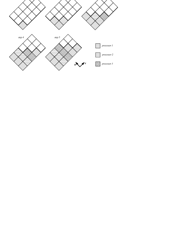
Figure 8: An illustration of the technique suggested to parallelize a characteristic code. In this example, three processors are available to simultaneously solve the equations. We subdivide the grid into blocks of equal area, and assign blocks to individual processors as shown in the figure. The heavy line drawn on the grid at step $i$ represents the surface where initial data will be available at step $i+1$. Before step one, there is only a single block where sufficient initial data is available to solve the equations, hence only one processor is active then. After step one there are two unsolved blocks that can be evolved, and thus two processors become active; and so on, until the “pipeline” of processors is full.

5 Tests & Results

In this section we present results from two evolutions obtained using the 1D characteristic AMR code described in the previous sections. The first example models a black hole interacting with an initially outgoing pulse of massive scalar field energy. The relatively large mass term we use, in conjunction with the compactified radial $x$ coordinate, causes a wide range of relevant scales to develop at late times, and we show that the algorithm is able to track these features with reasonable accuracy via comparison with results from unigrid evolution. The second example shows a near-critical collapse[32] of the massless scalar field. For reasons we will explain below, our coordinate system is not well suited to studying this kind of critical phenomena, and hence the example is not very close to criticality. Nevertheless, we are close enough to demonstrate that the algorithm can also adapt to the very small length scales that develop from ingoing initial data.

5.1 Massive scalar field - black hole interaction

For the first example, we specify $\Psi$ along $v=0$ as follows:

$$\Psi(v=0,x) = Ax(1-x/x_{1})^{4}(1-x/x_{2})^{4},\ \ \ x_{1}<x<x_{2},$$ (31)

$$= 0\ \ \ {\rm elsewhere},$$

choose $x_{1}=0.15$, $x_{2}=0.25$, $A=5\rm{x}10^{3}$ and the mass parameter $m=5$. We set $g(x=1,v=0)=0.2$, so that the asymptotic mass of the spacetime is $0.1$; the initial ($v=0$) black hole mass is $\approx 0.063$, indicating that the scalar field contributes $\approx 0.037$ to the initial mass of the spacetime. We ran the simulation to $v=10$, by which time the black hole mass had grown to roughly $0.068$ due to accretion of scalar field energy. First, to demonstrate the correctness of our solution to the finite difference equations, in Fig. 9 we show the convergence factor for the scalar field $Q_{\Psi}$

$$Q_{\Psi}=\frac{||\Psi_{4h}-\Psi_{2h}||_{2}}{||\Psi_{2h}-\Psi_{h}||_{2}},$$ (32)

computed using solutions from 3 different resolutions of unigrid simulations. $\Psi_{4h}$ has 1025 points in $x$, $\Psi_{2h}$ 2049, and $\Psi_{h}$ 4097. The Courant factor is $0.25$ in all cases; i.e. $\Delta v=0.25\Delta x$. That $Q_{\Psi}$ is around $4$ for most of the simulation indicates that we are seeing second order convergence, as expected (and that $Q_{\Psi}$ eventually starts to deviate from $4$ is also not unexpected—accumulating numerical errors, especially in our compactified coordinate system, will eventually cause any finite resolution simulation to move away from the convergent regime). For brevity we do not show convergence factors for the other fields; they also exhibit second order convergence. To demonstrate the accuracy of the adaptive code, we first show a comparson between a solution generated with AMR to the finest unigrid solution, and then present some results from a convergence test.

5.1.1 Comparison between AMR and unigrid solutions

For the comparison between the AMR and unigrid results, the parameters for the AMR run were set so that the base level (2) has $513$ points (hence the shadow level (1) has $257$ points), and the maximum allowed TE is such that early on (in $v$) during the evolution the finest level is $5$, giving the same resolution locally as that of the finest unigrid simulation. At late times during the adaptive run additional levels are introduced to track the outgoing pulse (whose width shrinks due to the radial coordinate we use)—see Fig. 10 for several snapshots of $\Psi$ along $v={\rm const.}$ surfaces during evolution, Fig. 11 for the maximum level as a function of $x$ at the same instants of $v$ shown in Fig. 10, and Fig. 12 for a plot of the maximum level in the hierarchy over all $x$ as a function of $v$. To gauge the quality of the adaptive solution, we use the highest resolution unigrid solution for $\Psi$ as a benchmark, and compare this solution to the lower resolution unigrid and adaptive results. Fig. 13 shows the $\ell_{2}$ norm (computed along $v={\rm const.}$ slices of the spacetime) of these differences, and Fig. 14 plots $\Psi(x,v=10)$ from the four simulations near the leading edge of the pulse, for visual comparison. Fig. 13 demonstrates that early on the adaptive solution gives slightly worse results than the lower resolution unigrid solution, which is not too surprising as the AMR solution only covers a portion of the computational domain with comparable or higher resolution. However, at late times the adaptive solution starts to outperform the coarser unigrid solutions as the AMR is able to keep the narrowing pulse well resolved.

5.1.2 AMR convergence test

For a separate convergence test of the AMR code we ran three simulations with the same initial data as described above, varying the base grid resolution and maximum allowed truncation error to mimic doubling the resolution from one run to the next. Specifically, the lower resolution simulation had 257 points in the base level (2) with a maximum TE of $\tau_{4h}$, the medium resolution run had a base grid of 513 points and a maximum TE of $\tau_{2h}=\tau_{4h}/4$, while the higher resolution simulation had a base grid of 1025 points and a maximum TE of $\tau_{h}=\tau_{4h}/16$. However, due to limited available computer resources we restricted the maximum depth of the hierarchy to 7 for these three runs (at this stage our code is not memory efficient, and the high resolution run was using most of the available memory nearing the end of the simulation). Note that this scheme for convergence testing an AMR code will not produce identical grid hierarchies that differ only in resolution, because the truncation error estimate used in each numerical simulation will not scale exactly as the leading order part of the actual truncation error, which decreases by a factor of 4 each time the mesh spacing is halved for a second order accurate scheme. Nevertheless, if the test were to show non-convergent results it would be a clear indication of problems with the implementation. Fig. 15 below shows the convergence factor for $\Psi$ (where to calculate $Q_{\Psi}$ as in (32) we first interpolated the solutions to identical uniform grids). Early on we get a convergence factor that is closer to first than second order convergence. The primary reason for this appears to be grid-boundary “noise” generated at parent-child interfaces, and as discussed in Sec. 4.1.1 our current interpolation/dissipation scheme is not yet very effective at reducing this noise. Later on in the simulation the convergence behavior appears to improve significantly (and become unrealistically high), however this is mostly because we had to limit the maximum level to 7. At late times this is not sufficient to maintain the desired TE (see Fig. 11 for the level structure generated by the AMR run described in the previous section, which had a base resolution equivalent to that of the medium resolution simulation here), and the solutions start to drift away from the convergent regime. In fact, by $v=10$ the lower resolution run had accumulated significant phase errors in $\Psi$, whereas the medium and high resolution solutions were still roughly in phase, which gives some explanation for the anomalously high value of $Q_{\Psi}$ (32) in this case.

5.2 Massless scalar field critical collapse

For a second, brief example, we consider the near-critical collapse of an initially ingoing pulse of the massless scalar field:

$$\Psi(v,x=1) = A(1-v/v_{1})^{4}(1-v/v_{2})^{4},\ \ \ v_{1}<v<v_{2},$$ (33)

$$= 0\ \ \ {\rm elsewhere},$$

and set $v_{1}=0.01$, $v_{2}=0.11$ and $g(x=1,v=0)=0$. $A$ is tuned (via a bisection search) so that the collapsing pulse is close to the threshold of black hole formation. As mentioned before, the coordinates we use are not well suited to studying type II critical collapse, where one should be able to form arbitrarily small black holes in the super-critical regime. The reason is that in our coordinate system, a non-zero initial value $g(x=1,v=0)=2m_{0}$ describes a spacetime containing a black hole of mass $m_{0}$ (assuming $\Psi(x,v=0)=0$). Truncation error effects in the integration of $g(x=1,v)$, and subsequent evolution in $x$, causes small errors in $g$ that effectively behave as if a small black hole (of size proportional to the TE) had been present in the initial data. This is not a problem for unigrid evolution, as the erroneous black hole is typically smaller than the grid spacing; however during a critical evolution where arbitrarily small scales unfold, and refinement resolves these scales, this black hole is eventually revealed. Thus the resolution of the initial data at ${I}^{-}$ places a limit on how close to critical we can evolve. For this example we chose a base (level $2$) resolution of $2049$ in $x$ (with $\Delta v=0.25\Delta x$); then the smallest black hole we can form is on the order of $10^{-4}$, which is roughly $1/2$ the size of a base-level cell in $x$. Fig. 16 shows several snapshots of $\Psi/r$ from the evolution of the nearest-to-critical sub-critical amplitude we found, and Fig. 17 shows the corresponding level structure.

Figure 9: The convergence factor $Q_{\Psi}$ (32) from unigrid evolution of the black hole-massive scalar field initial data.

Figure 10: $\Psi(x)$ along several $v={\rm const.}$ slices of the spacetime, from the adaptive black hole-massive scalar field simulation discussed in section 5.1.1. The position of the excision surface is denoted by a vertical dashed line, and is always kept a distance of $0.025$ in $x$ inside the apparent horizon; the scalar field is set to zero inside the excision surface. The scalar field pulse is initially outgoing, and the higher-frequency components of the field continue to travel outward at the speed of light. The non-zero mass term in the scalar field equation of motion causes lower frequency components of the field to travel at speeds less that $1$; these trail the leading pulse of the field, and interact more strongly with the black hole. See Fig. 11 below for a plot of the maximum AMR level along the same slices shown here to see how the AMR algorithm correctly tracks the outgoing, higher-frequency components of the solution.

Figure 11: Maximum level of the hierarchy from the adaptive black hole-massive scalar field simulation discussed in section 5.1.1, at the same slices of the computational domain shown in Fig. 10.

Figure 12: Maximum level of the adaptive hierarchy along $v={\rm const.}$ slices of the spacetime, from the adaptive black hole-massive scalar field simulation discussed in section 5.1.1.

Figure 13: Comparison of $\Psi(x,v={\rm const.})$ between the highest resolution unigrid simulation ($\Psi_{h}$), and lower resolutions unigrid simulations ($\Psi_{2h}$ and $\Psi_{4h}$) and adaptive simulation ($\Psi_{ad}$) described in in section 5.1.1. The unigrid $h$ ($2h,4h$) simulation has $4097$ ($2049,1025$) points in $x$, while level $5$ of the AMR run has the same resolution as the $h$ unigrid run (see Fig. 11). This figure shows that at early times, both the $2h$ and $4h$ unigrid simulations perform slightly better than the adaptive run, compared to the $h$ unigrid solution; however at late times the adaptive code starts to outperform the lower resolution unigrid runs, as the AMR tracks the ever-narrowing outgoing pulse (see Fig. 10). See Fig. 14 below for plots of $\Psi$ from the four solutions at $v=10$.

Figure 14: $\Psi(x)$ from the adaptive and three unigrid solutions, at $v=10$ of the black hole-massive scalar field simulation (section 5.1.1). We only show a small range of the $x$ coordinate domain (compare Fig. 10), as this region shows the largest disagreement among the four simulations. The unigrid $h$ ($2h,4h$) simulation has $4097$ ($2049,1025$) points in $x$, while level $5$ of the AMR run has the same resolution as the $h$ unigrid run (see the last frame of Fig. 11).

Figure 15: The convergence factor $Q_{\Psi}$ (32) from AMR evolutions of the black hole-massive scalar field initial data. The lack of second order convergence is primarily due to inadequate dissipation of high-frequency “noise” generated at parent-child interfaces, and the anomalously high convergence factor at later times is due to a significant phase error developing in the solution from the lowest resolution run compared to the two higher resolution runs; see the text in section 5.1.2 for further discussion.

Figure 16: $\Psi(x)/r(x)$ along several $v={\rm const.}$ slices of the spacetime, from a sub-critical, massless scalar field evolution (with purely ingoing initial data, i.e. $\Psi(x,v=0)=0$). The first four plots above correspond to slices where $\Psi(x)/r(x)$ has attained a local maximum or minimum at the origin; the first two of these would be present in the weak field regime, in the next two we are beginning to see the first half-echo of the critical solution (one feature of which is that the central value of the scalar field oscillates between approximately $\pm 0.6$ during each self-similar echo). In the last frame the scalar field is dispersing.

Figure 17: The maximum level of the hierarchy along the slices of the near-critical simulation shown in Fig. 16

6 Conclusion

In this paper we have introduced a new algorithm that can be used to add an adaptive mesh refinement framework to a characteristic evolution code. The algorithm is similar to the Berger and Oliger algorithm for Cauchy codes, and shares many of its desirable features, including dynamical regridding via local truncation error estimates, efficient use of computational resources via the recursive evolution scheme, and in principle it does not require modifications to the underlying unigrid finite difference scheme. As discussed in the introduction, we believe AMR is essential to achieve accurate results from simulations in many general relativistic scenarios. Based upon the early success of this AMR technique with the one dimensional code presented here, we think it would be well worth the effort to apply the method to higher dimensional problems of interest.

7 Acknowledgments

We thank Matthew Choptuik for valuable insights. FP would like to acknowledge NSERC, The Izaak Walton Killam Fund, Caltech’s Richard Chase Tolman Fund and NSF PHY-0099568 for financial support. Computations were performed on the vn.physics.ubc.ca Beowulf cluster (supported by CFI and BCKDF) L.L. thanks PIMS and CITA for partial finantial support and the California Institute of Technology for hospitality where the last stages of this work were completed.

References

- [1] J. Winicour, in: N. Troyani, M. Cerrolaza (Eds.), Proceedings the 5th Internationa Congress of Numerical Methods in Engeneering and Applied Science, CIMENICS 2000., 2000.
- [2] L. Lehner, Numerical relativity: A review, Class. Quant. Grav. 18 (2001) R25–R86.
- [3] H. Bondi, M. van der Burg, A. Metzner, Gravitational waves in general relativity VII. Waves from axi-symmetric isolated systems, Proc. R. Soc. London Ser. A (270) (1962) 103.
- [4] R. Sachs, Proc. R. Soc. A 270 (1962) 103.
- [5] E. T. Newman, R. Penrose, J. Math. Phys. 3 (1962) 566.
- [6] L. Tamburino, J. Winicour, Phys. Rev. 150 (1966) 1039.
- [7] J. Winicour, Characteristic evolution and matching, Living Rev. Rel. 1 (1998) 5.
- [8] P. Tod, in: H. Friedrich, J. Frauendiener (Eds.), Proceedings of the Conformal Structure of Spacetimes, Springer Verlag, Berlin, 2002.
- [9] R. S. Hamade, J. M. Stewart, The spherically symmetric collapse of a massless scalar field, Class. Quant. Grav. 13 (1996) 497–512.
- [10] D. Garfinkle, Choptuik scaling in null coordinates, Phys. Rev. D51 (1995) 5558–5561.
- [11] V. Husain, M. Olivier, Scalar field collapse in three-dimensional ads spacetime, Class.Quant.Grav. 18 (2001) L1–L10.
- [12] L. M. Burko, Structure of the black hole’s cauchy horizon singularity, Phys. Rev. Lett. 79 (1997) 4958–4961.
- [13] P. R. Brady, C. M. Chambers, S. M. C. V. Goncalves, Phases of massive scalar field collapse, Phys. Rev. D56 (1997) 6057–6061.
- [14] R. Gomez, J. S. Welling, J. Winicour, R. A. Isaacson, Numerical relativity on null cones In Philadelphia 1985, proceedings, dynamical spacetimes and numerical relativity 236-255.
- [15] N. T. Bishop, R. Gomez, L. Lehner, M. Maharaj, J. Winicour, High-powered gravitational news, Phys. Rev. D56 (1997) 6298–6309.
- [16] R. Gomez, L. Lehner, R. L. Marsa, J. Winicour, Moving black holes in 3d, Phys. Rev. D57 (1998) 4778–4788.
- [17] R. A. d’Inverno, M. R. Dubal, E. A. Sarkies, Cauchy-characteristic matching for a family of cylindrical vacuum solutions possessing both gravitational degrees of freedom, Class. Quant. Grav. 17 (2000) 3157.
- [18] R. Bartnik, Einstein equations in the null quasi-spherical gauge, Class. Quant. Grav. 14 (1997) 2185–2194.
- [19] F. Siebel, J. A. Font, E. Muller, P. Papadopoulos, Simulating the dynamics of relativistic stars via a light- cone approach, Phys. Rev. D65 (2002) 064038.
- [20] N. T. Bishop, R. Gomez, L. Lehner, M. Maharaj, J. Winicour, The incorporation of matter into characteristic numerical relativity, Phys. Rev. D60 (1999) 024005.
- [21] N. Bishop, R. Gómez, L. Lehner, J. Winicour, Phys. Rev. D. 54 (1996) 6153.
- [22] L. Lehner, A dissipative algorithm for wave-like equations in the characteristic formulation, J. Comp. Phys. 149 (1999) 59-74.
- [23] R. Gomez, Gravitational waveforms with controlled accuracy, Phys. Rev. D64 (2001) 024007.
- [24] S. Hawking, G. Ellis, The Large Scale Structure of Space-Time, Cambridge University Press, Cambridge, 1974.
- [25] R. Gomez, R. L. Marsa, J. Winicour, Black hole excision with matching, Phys. Rev. D56 (1997) 6310–6319.
- [26] J. Thornburg., Coordinates and boundary conditions for the general relativistic initial data problem, Class. Quant. Grav 4 (1987) 1119.
- [27] W. R., General Relativity, The University of Chicago Press, Chicago, 1984.
- [28] M. Berger, J. Oliger, Adaptive mesh refinement for hyperbolic partial differential equations, J. Comp. Phys. 53 (1984) 484.
- [29] R. A. Isaacson, J. S. Welling, J. Winicour, Null cone computation of gravitational radiation, J. Math. Phys. 24 (1983) 1824–1834.
- [30] F. Pretorius, Numerical simulations of gravitational collapse, Ph.D. thesis, Univ. of British Columbia (2002).
- [31] H. Kreiss, J. Oliger, Methods for the approximate solution of time dependent problems, Global Atmospheric Research Programme, Publications Series No. 10. .
- [32] M. Choptuik, Universality and scaling in gravitational collapse of a massless scalar field, Phys. Rev. Lett. 70 (1993) 9.
- [33] D. Garfinkle, G. Duncan, Scaling of curvature in sub-critical gravitational collapse, Phys. Rev. D 58 (1998) 064024.