Axisymmetric core collapse simulations using characteristic numerical relativity

Abstract

We present results from axisymmetric stellar core collapse simulations in general relativity. Our hydrodynamics code has proved robust and accurate enough to allow for a detailed analysis of the global dynamics of the collapse. Contrary to traditional approaches based on the 3+1 formulation of the gravitational field equations, our framework uses a foliation based on a family of outgoing light cones, emanating from a regular center, and terminating at future null infinity. Such a coordinate system is well adapted to the study of interesting dynamical spacetimes in relativistic astrophysics such as stellar core collapse and neutron star formation. Perhaps most importantly this procedure allows for the unambiguous extraction of gravitational waves at future null infinity without any approximation, along with the commonly used quadrupole formalism for the gravitational wave extraction. Our results concerning the gravitational wave signals show noticeable disagreement when those are extracted by computing the Bondi news at future null infinity on the one hand and by using the quadrupole formula on the other hand. We have strong indication that for our setup the quadrupole formula on the null cone does not lead to physical gravitational wave signals. The Bondi gravitational wave signals extracted at infinity show typical oscillation frequencies of about 0.5 kHz.

I Introduction

Supernova core collapse marks the final stage of the stellar evolution of massive stars. If the core collapse and/or the supernova explosion are nonspherical, part of the liberated gravitational binding energy will be emitted in the form of gravitational waves. According to estimates from numerical simulations, the total energy emitted in gravitational waves in such events can be as high as $10^{-6}M_{\odot}c^{2}$ Müller (1982); Mönchmeyer et al. (1991); Zwerger and Müller (1997); Dimmelmeier et al. (2002a). Nonsphericity can be caused by the effects of rotation, convection and anisotropic neutrino emission leading either to a large-scale deviation from spherical symmetry or to small-scale statistical mass-energy fluctuations (for a review, see e.g., Müller (1998)). Supernovae have always been considered among the most important sources of gravitational waves to be eventually detected by the current or next generations of gravitational wave laser interferometers. If detected, the gravitational wave signal could be used to probe the models of core collapse supernovae and to study the formation of neutron stars.

Earlier studies of axisymmetric supernova core collapse were performed using Newton’s law of gravity Mönchmeyer et al. (1991); Yamada and Sato (1994); Zwerger and Müller (1997). More recently, effects of general relativity have been included under the simplifying assumption of a conformally flat spatial metric Dimmelmeier et al. (2001); Dimmelmeier et al. (2002b, a). In all existing works gravitational waves are not calculated instantly within the numerical simulation, but they are extracted a posteriori using the approximation of the quadrupole formalism which links gravitational waves to the change of the quadrupole moment of the simulated matter distribution.

In this paper we present first results of a project aimed at studying the dynamics of stellar core collapse by means of numerical simulations in full general relativity. The trademark of our approach is the use of the so-called characteristic formulation of general relativity (see Winicour (2001) for a review), in which spacetime is foliated with a family of outgoing light cones emanating from a regular center. Due to a suitable compactification of the global spacetime future null infinity is part of our finite numerical grid where we can unambiguously extract gravitational waves. This remarkable feature is the main motivation behind our particular choice of slicing and coordinates, which clearly departs from earlier investigations. We note, however, that we have not modeled the detailed microphysics of core collapse supernovae, which is beyond the scope of the present investigation. Instead, we only take into account the most important features for both, the gravitational field and the hydrodynamics, and those will be introduced in the upcoming section.

Characteristic numerical relativity has traditionally focused on vacuum spacetimes. In recent years the field has witnessed steady improvement, and robust and accurate three-dimensional codes are nowadays available, as that described in Bishop et al. (1997), which has been applied to diverse studies of black hole physics (e.g. Gómez et al. (1998)). In black hole spacetimes, only the geometry outside a horizon is covered by the foliation of light cones. This is is not the case for neutron stars or gravitational collapse spacetimes which must include a regular origin. Up to now, characteristic vacuum codes with a regular center have only been studied in spherical symmetry and in axisymmetry Gómez et al. (1994).

The inclusion of relativistic hydrodynamics into the characteristic approach along with the implementation of high-resolution shock-capturing (HRSC) schemes in the solution procedure was first considered by Papadopoulos and Font Papadopoulos and Font (2000); Papadopoulos and Font (1999a); Font (2000). First applications in spherical symmetry were presented, dealing with black hole accretion Papadopoulos and Font (1999b) and the interaction of relativistic stars with scalar fields Siebel et al. (2002a) as simple models of gravitational waves. Axisymmetric studies of the Einstein-perfect fluid system were first discussed in Siebel et al. (2002b). In this reference we presented an axisymmetric, fully relativistic code which could maintain long-term stability of relativistic stars and which allowed us to perform mode-frequency computations and the gravitational wave extraction of perturbed stellar configurations. The core collapse simulations presented in the current paper are based on this code, which is described in detail in Ref. Siebel et al. (2002b).

The paper is organized as follows: In Sec. II we describe the mathematical and numerical framework we use in the simulations. Section III deals with presenting the initial data of the unstable equilibrium stellar configurations we evolve. Section IV is devoted to discuss the numerical simulations, with emphasis on the collapse dynamics. In Sec. V we analyze the corresponding gravitational wave signals. A summary and a discussion of our results are given in Sec. VI. Finally, tests to calibrate the code in simulations of core collapse are collected in the Appendix.

II Framework and implementation

We only briefly repeat the basic properties of our approach here. The interested reader is referred to our previous work Siebel et al. (2002b) for more details concerning the mathematical setup and the numerical implementation. As described in Ref. Siebel et al. (2002b), we work with the coupled system of Einstein and relativistic perfect fluid equations

$$G_{ab} = \kappa T_{ab}\,,$$ (1)

$$\nabla_{a}T^{ab} = 0\ ,$$ (2)

$$\nabla_{a}J^{a} = 0,$$ (3)

where $\nabla_{a}$, as usual, denotes the covariant derivative. The energy-momentum tensor for a perfect fluid $T_{ab}$ takes the form.

$$T_{ab}=\rho hu_{a}u_{b}+pg_{ab}.$$ (4)

Here $\rho$ denotes the rest mass density, $h=1+\epsilon+\frac{p}{\rho}$ is the specific enthalpy, $\epsilon$ is the specific internal energy, and $p$ is the pressure of the fluid. The four-vector $u^{a}$, the 4-velocity of the fluid, fulfills the normalization condition $g_{ab}u^{a}u^{b}=-1$. The four-current $J^{a}$ is defined as $J^{a}=\rho u^{a}$. Using geometrized units ($c=G=1$) the coupling constant in the field equations is $\kappa=8\pi$. We further use units in which $M_{\odot}=1$. Moreover, an equation of state (EoS) needs to be prescribed, $p=p(\rho,\epsilon)$, as we discuss in Sec. II.3 below.

Our numerical implementation of the field equations of general relativity is based on a spherical null coordinate system $(u,r,\theta,\phi)$. Here, $u$ denotes a null coordinate labeling outgoing light cones, $r$ is a radial coordinate, and $\theta$ and $\phi$ are standard spherical coordinates. Assuming axisymmetry, $\phi$ is a Killing coordinate. In order to resolve the entire radial range from the origin of the coordinate system up to future null infinity, we define a new radial coordinate $x\in[0,1]$. The radial coordinate $r$ is a function of the coordinate $x$, which can be adapted to the particular simulation. In this work, except where otherwise stated, we use a grid function $r(x)=100\tan({\frac{\pi}{2}x})$, for which the limit $x\to 1$ corresponds to $r\to\infty$. Moreover, in order to eliminate singular terms at the poles ($\theta=0,\pi$) we introduce the new coordinate $y=-\cos\theta$.

II.1 The characteristic Einstein equations

The geometric framework relies on the Bondi (radiative) metric Bondi et al. (1962)

$$ds^{2}=-\left(\frac{V}{r}e^{2\beta}-U^{2}r^{2}e^{2\gamma}\right)du^{2}-2e^{2\beta}dudr$$ (5)

$$- 2Ur^{2}e^{2\gamma}dud\theta+r^{2}(e^{2\gamma}d\theta^{2}+e^{-2\gamma}\sin^{2}\theta d\phi^{2}).$$

We substitute the metric variables $(\beta,V,U,\gamma)$ by the new set of metric variables $(\beta,S,\hat{U},\hat{\gamma})$,

$$S = \frac{V-r}{r^{2}},$$ (6)

$$\hat{U} = \frac{U}{\sin\theta},$$ (7)

$$\hat{\gamma} = \frac{\gamma}{\sin^{2}\theta},$$ (8)

in order to obtain regular expression in the Einstein equations in particular at the polar axis. The origin of the coordinate system $r=0$ is chosen to lie on the axis of our axisymmetric stellar configurations, where we describe boundaries and falloff conditions for the metric fields. The complete set of Einstein equations reduces to a wave equation for the quantity $\hat{\gamma}$ (see Eq. (8)) and a hierarchical set of hypersurface equations for the quantities $(\beta,\hat{U},S)$ to be solved along the light rays $u=\text{const}$. The particular form of these equations is explicitly given in Ref. Siebel et al. (2002b).

II.2 The relativistic perfect fluid equations

The axisymmetric general relativistic fluid equations on the light cone, Eqs. (2) and (3), are written as a first-order flux-conservative, hyperbolic system for the state-vector ${\bf U}=(U^{u},U^{x},U_{y},U^{4})=(T^{uu},T^{ux},T^{u}_{~{}y},J^{u})$. Following our previous work Siebel et al. (2002a) we have not included the metric determinant in the definition of the state vector. Explicitly, in the coordinates $(x^{0},x^{1},x^{2},x^{3})=(u,x,y,\phi)$, we obtain

$$\partial_{0}U^{u}+\partial_{j}F^{ju} = S^{u}\ ,$$ (9)

$$\partial_{0}U^{x}+\partial_{j}F^{jx} = S^{x}\ ,$$ (10)

$$\partial_{0}U_{y}+\partial_{j}F^{j}_{~{}y}\ = S_{y}\ ,$$ (11)

$$\partial_{0}U^{4}+\partial_{j}F^{j4} = S^{4}.$$ (12)

The flux vectors are defined as

$$F^{ju} = T^{ju}\ ,$$ (13)

$$F^{jx} = T^{jx}\ ,$$ (14)

$$F^{j}_{~{}y} = T^{j}_{~{}y}\ ,$$ (15)

$$F^{j4} = J^{j}\ ,$$ (16)

and the corresponding source terms read

$$S^{a} = -\big{(}\ln(\sqrt{-g})\big{)}_{,b}\ T^{ab}+g^{ab}\ S_{b}+T^{c}_{~{}b}(g^{ab})_{,c},\hskip 10.0pt$$ (17)

$$S_{a} = -\frac{1}{2}\rho hu_{c}u_{d}(g^{cd})_{,a}+p-\big{(}\ln(\sqrt{-g})\big{)}_{,b}\ T^{b}_{~{}a}\ ,\hskip 10.0pt$$ (18)

$$S^{4} = -\big{(}\ln(\sqrt{-g})\big{)}_{,b}\ J^{b}\ ,\hskip 10.0pt$$ (19)

wherein a comma is used to denote a partial derivative.

The fluid update from time $u^{n}$ to $u^{n+1}$ at a given cell $i,j$ is given by

$${\mathbf{U}}_{i,j}^{n+1}={\mathbf{U}}_{i,j}^{n} - \frac{\Delta u}{\Delta x}(\widehat{{\mathbf{F}}}_{i+1/2,j}-\widehat{{\mathbf{F}}}_{i-1/2,j})$$ (20)

$$- \frac{\Delta u}{\Delta y}(\widehat{{\mathbf{G}}}_{i,j+1/2}-\widehat{{\mathbf{G}}}_{i,j-1/2})$$

$$+ \Delta u{\mathbf{S}}_{i,j}\,,$$

where the numerical fluxes, $\widehat{{\mathbf{F}}}$ and $\widehat{{\mathbf{G}}}$, are evaluated at the cell interfaces according to a flux-formula, the one due to Harten, Lax and van Leer (HLL) in our case Harten et al. (1983). The characteristic information of the Jacobian matrices associated with the hydrodynamical fluxes, which is used in this flux formula, was presented elsewhere Papadopoulos and Font (1999b). We use the monotonized central difference slope limiter by van Leer van Leer (1977) for the reconstruction of the hydrodynamical quantities at the cell interfaces needed in the solution of the Riemann problems. This scheme is second order accurate in smooth monotonous parts of the flow and gives improved results compared to the MUSCL scheme applied in Siebel et al. (2002b) (for an independent comparison, see Font et al. (2002)).

II.3 Equation of state

We use a hybrid EoS which includes the effect of stiffening at nuclear densities and the effect of thermal heating due to the appearance of shocks. Such an EoS was first considered by Janka et al. Janka et al. (1993), and has been used for core collapse simulations both, using Newtonian gravity Zwerger and Müller (1997); Rampp et al. (1998) and in general relativity under the assumption of conformal flatness Dimmelmeier et al. (2001); Dimmelmeier et al. (2002b, a).

In our EoS the total pressure consists of a polytropic part, which takes into account the contribution from the degenerate electron gas, as well as the nuclear forces (at high densities), and a thermal part due to the heating of the material by a shock, $p=p_{\mathrm{p}}+p_{\mathrm{th}}$. More precisely, the polytropic part follows the relation

$$p_{p}=\left\{\begin{array}[]{ll}\kappa_{1}\rho^{\Gamma_{1}},&\text{for $\rho\leq\rho_{\mathrm{n}}$},\\ \kappa_{2}\rho^{\Gamma_{2}},&\text{for $\rho>\rho_{\mathrm{n}}$},\end{array}\right.$$ (21)

where we assume a nuclear density $\rho_{\mathrm{n}}=2\times 10^{14}\ \text{g}\ \text{cm}^{-3}$. For a degenerate relativistic electron gas $\Gamma=\Gamma_{\mathrm{ini}}=4/3$ and $\kappa=4.8974894\times 10^{14}\ [\text{cgs}]$. To model the physical processes which lead to the onset of the collapse, we reduce the effective adiabatic index from $\Gamma$ to $\Gamma_{1}$ setting $\kappa_{1}=\kappa$ at the initial slice. Moreover, to model the stiffening of the EoS at nuclear densities, we assume $\Gamma_{2}=2.5$. The value of the polytropic constant $\kappa_{2}$ follows from the requirement that the pressure is continuous at nuclear density. The thermodynamically consistent internal energy distribution reads

$$\epsilon_{\mathrm{p}}=\left\{\begin{array}[]{ll}\frac{\kappa_{1}}{\Gamma_{1}-1}\rho^{\Gamma_{1}-1},&\text{for $\rho\leq\rho_{\mathrm{n}}$},\\ \frac{\kappa_{2}}{\Gamma_{2}-1}\rho^{\Gamma_{2}-1}+E,&\text{for $\rho>\rho_{\mathrm{n}}$}.\end{array}\right.$$ (22)

The requirement that $\epsilon_{\mathrm{p}}$ is continuous at nuclear density leads to

$$E=\frac{(\Gamma_{2}-\Gamma_{1})\kappa_{1}}{(\Gamma_{2}-1)(\Gamma_{1}-1)}\ \rho_{\mathrm{n}}^{\Gamma_{1}-1}.$$ (23)

For the thermal contribution to the total pressure, we assume an ideal fluid EoS

$$p_{\mathrm{th}}=(\Gamma_{\mathrm{th}}-1)\rho\epsilon_{\mathrm{th}},$$ (24)

with an adiabatic index $\Gamma_{\mathrm{th}}=\frac{3}{2}$ describing a mixture of relativistic and non-relativistic gases. The internal thermal energy $\epsilon_{\mathrm{th}}$ is simply obtained from

$$\epsilon_{\mathrm{th}}=\epsilon-\epsilon_{\mathrm{p}}.$$ (25)

We can summarize the EoS in a single equation:

$$p = \kappa\left(1-\frac{\Gamma_{\mathrm{th}}-1}{\Gamma-1}\right)\rho^{\Gamma}+(\Gamma_{\mathrm{th}}-1)\rho\epsilon$$ (26)

$$- \frac{(\Gamma_{\mathrm{th}}-1)(\Gamma-\Gamma_{1})}{(\Gamma_{2}-1)(\Gamma_{1}-1)}\kappa\rho_{\mathrm{n}}^{\Gamma-1}\rho,$$

where $\Gamma$ and $\kappa$ change discontinuously at nuclear density $\rho_{\mathrm{n}}$ from $\Gamma_{1}$ to $\Gamma_{2}$ and $\kappa_{1}$ to $\kappa_{2}$. For the sound speed $c_{s}$, we obtain

$$hc_{s}^{2}=\frac{1}{\rho}(\Gamma p_{\mathrm{p}}+\Gamma_{\mathrm{th}}p_{\mathrm{th}}).$$ (27)

II.4 Recovery of the primitive variables

After the time update of the state-vector of hydrodynamical quantities, the primitive variables $(\rho,u^{x},u_{y},\epsilon)$ have to be recomputed. The relation between the two sets of variables is not in closed algebraic form. Using the hybrid EoS, such recovery is performed as follows: With the definition $S^{ab}=g^{cd}T^{a}_{~{}c}T^{b}_{~{}d}$, we obtain Papadopoulos and Font (1999a)

$$S^{uu}=\Big{(}\frac{p}{\rho}-1-\epsilon\Big{)}\Big{(}\frac{p}{\rho}+1+\epsilon\Big{)}(J^{u})^{2}+p^{2}g^{uu},$$ (28)

where in our null coordinate system $g^{uu}=0$. Let $F(\rho,\epsilon)=\frac{p}{\rho}$. From Eqs. (26), (28) and the definition of the specific enthalpy $h$ we obtain the 3 equations for the 3 unknowns $F$, $\rho$ and $\epsilon$

$$F(\rho,\epsilon) = \sqrt{L+(1+\epsilon)^{2}},$$ (29)

$$F(\rho,\epsilon) = (\Gamma_{th}-1)\epsilon+G(\rho),$$ (30)

$$\rho = H(1+\epsilon+F(\rho,\epsilon)).$$ (31)

In these equations we made use of the abbreviations

$$L = \frac{S^{uu}}{(J^{u})^{2}},$$ (32)

$$G(\rho) = \kappa\Big{(}1-\frac{\Gamma_{th}-1}{\Gamma-1}\Big{)}\rho^{\Gamma-1}$$ (33)

$$-\frac{(\Gamma_{th}-1)(\Gamma-\Gamma_{1})}{(\Gamma_{2}-1)(\Gamma_{1}-1)}\kappa\rho_{n}^{\Gamma-1},$$

$$I = \frac{(J^{u})^{2}}{T^{uu}}.$$ (34)

From Eqs. (29)-(31) we deduce a single implicit equation for the rest mass density $\rho$

$$f_{\text{imp}}(\rho):=\Big{(}\frac{\rho}{I}\Big{)}^{2}-2\frac{\rho}{I}(1+\epsilon)-L=0,$$ (35)

where we consider the internal energy as function of $\rho$

$$\epsilon=\frac{1}{\Gamma_{th}}\Big{(}\frac{\rho}{I}-(1+G(\rho))\Big{)}.$$ (36)

We solve Eq. (35) for $\rho$ with a Newton-Raphson method.

III Initial data

In the final stage of the evolution of massive stars, the iron core in the stellar center has a central density of about $\rho_{c}=10^{10}\ \text{g}\ \text{cm}^{-3}$ when it becomes dynamically unstable to collapse. As the pressure of the degenerate relativistic electrons is by far the most important contribution to the total pressure, the pressure in the iron core can be approximated by a $\Gamma=\frac{4}{3}$ polytropic EoS. In order to obtain an initial model for the iron core, we solve the Tolman-Oppenheimer-Volkoff equation Siebel et al. (2002b) with the above central density, which corresponds to $\rho_{c}=1.62\times 10^{-8}$ in code units ($c=G=M_{\odot}=1$).

To initiate the gravitational collapse we set the adiabatic index $\Gamma_{1}$ in the hybrid EoS (26) to a value of $1.30$, which mimics the softening of the EoS due to capture of electrons and due to the endothermic photodisintegration of heavy nuclei. The chosen value is within the interval range analyzed in previous studies of rotational core collapse based on Newtonian physics Zwerger and Müller (1997) and on the conformal flat metric approximation of general relativity Dimmelmeier et al. (2001); Dimmelmeier et al. (2002b, a).

Since rotation is not included in our current implementation, the equilibrium initial models of the iron core are spherically symmetric. Furthermore, in the evolution of these data during the phases of collapse, bounce, and beyond, spherical symmetry is conserved. Therefore, since we are mainly interested in simulating core collapse as a source of gravitational waves, we add non-radial perturbations on top of the spherical data. Our analysis is thus restricted to collapse scenarios where the effects of rotation are unimportant and in which stellar evolution has led to asymmetries in the iron core, e.g. due to convection Bazan and Arnett (1994). The strongest gravitational wave signals are expected for perturbations of quadrupolar form. Hence, we further restrict our analysis to this case, varying the form and amplitude of the perturbation in the initial data. We note that the evolution of such data, however, can produce an arbitrary type of perturbation within the class of the imposed symmetry.

We have classified the different models as follows: In case $\mathfrak{A}$ the spherical model is unperturbed; in case $\mathfrak{B}$ we prescribe a perturbation of the rest mass density

$$\delta\rho=A\rho_{s}\sin\Big{(}\frac{\pi r^{2}}{R^{2}}\Big{)}y^{2},$$ (37)

where $\rho_{s}$ denotes the spherical density distribution. Finally, in case $\mathfrak{C}$ we prescribe a perturbation of the meridional velocity component

$$u_{y}=A\sin\Big{(}\frac{\pi r^{2}}{R^{2}}\Big{)}y.$$ (38)

In the above two equations $A$ is a free parameter describing the amplitude of the perturbation, and $R$ denotes the radius of the iron core ($R=1.4\times 10^{3}$ km). We note in passing that in Siebel et al. (2002b) we already used a perturbation of the form $\mathfrak{C}$ to study quadrupolar oscillations of relativistic stars. We have further classified models $\mathfrak{B}$ and $\mathfrak{C}$ according to the amplitude $A$ of the perturbation (e.g. case $\mathfrak{C}01$ would correspond to an amplitude $A=0.1$).

Figure 1: Evolution of the central density for the collapse model $\mathfrak{B}01$ using a semilogarithmic scaling. During the collapse the central density increases by 4.5 orders of magnitude. When reaching supra-nuclear densities, the collapse is stopped as a consequence of the stiffening in the hybrid EoS at about $40$ ms after the collapse was initiated. The central density finally approaches a new equilibrium supra-nuclear value. Shortly after bounce, oscillations appear in the central density (see inset).

IV Core collapse dynamics

This section deals with the description of the global dynamics of our core collapse simulations. Relevant tests of the code which assess its suitability for such simulations are collected in the Appendix.

IV.1 Collapse and bounce

When evolving the initial models described in the previous section, the core starts to collapse. Fig. 1 shows the evolution of the central density for model $\mathfrak{B}01$ as a function of the Bondi time $u_{B}$. The lapse of Bondi time as seen by an observer at infinity is defined by

$$du_{B}=\omega e^{2H}du,$$ (39)

where $H=\lim_{r\to\infty}\beta$. The conformal factor $\omega$ relates the two-geometry of the Bondi metric

$$d\hat{s}^{2}=e^{2\gamma}d\theta^{2}+\sin^{2}\theta e^{-2\gamma}d\phi^{2}$$ (40)

to the two-geometry of a unit sphere

$$d\hat{s}_{B}^{2}=d\theta_{B}^{2}+\sin^{2}\theta_{B}d\phi_{B}^{2}.$$ (41)

as $d\hat{s}_{B}^{2}=\omega^{2}d\hat{s}^{2}$. When the central density reaches nuclear density at a Bondi time of about 40 ms, the pressure increases strongly according to Eq. (21). The central density grows further, but its increase is soon stopped. Afterwards, it drops below its maximum value, finally approaching a quasi-equilibrium supra-nuclear value when a “proto-neutron star” has formed in the central region note (2003).

Figure 2: Spacetime diagram for the collapse model $\mathfrak{A}$. Plotted is the lapse of proper time as a function of the radial coordinate $r$. The black solid lines correspond to a subset of the light curves by which we foliate the spacetime (there is one light cone after every 5 ms, where time is measured by an observer at the origin). The dashed curves correspond to different mass shells: $M=0.2M_{\odot},0.4M_{\odot},0.6M_{\odot},0.8M_{\odot},1.0M_{\odot},1.2M_{\odot}$. After about $40$ ms, a shock (thick solid line) forms in the interior region close to the origin. The diagram was obtained from a global simulation with 800 radial zones, extending the grid to future null infinity.

Figure 3: Snapshots of radial velocity profiles $u^{r}$, plotted as function of radius $r$ for the collapse model $\mathfrak{A}$. The snapshots are taken between $u_{B}=30$ ms and $u_{B}=45$ ms, with a delay of $1$ ms between subsequent outputs (the solid lines correspond to $u_{B}=30,35,40,45$ ms). The shock formation takes place at about 40 ms. In the outer part of the plotted region, the infall velocity of matter increases monotonically with time.

Fig. 2 shows a spacetime diagram for the core collapse simulation of model $\mathfrak{A}$ (the main aspects are similar for all our models). The diagram shows different mass shells and the location of the shock front (thick solid line). In order to localize the shock front, we search for coordinate locations where the $x$-component of the 4-velocity $u^{x}$ fulfills $u^{x}_{i}-u^{x}_{i+1}\geq s$, with $s$ being a threshold value for a velocity jump to be adapted (typical values for our simulations are $s=10^{-5}...10^{-4}$). In addition, to compute the mass inside a fixed radius, we make use of the relation

$$M=4\pi\int_{0}^{\infty}r^{2}e^{-2\beta}T_{ru}dr,$$ (42)

valid for the spherical collapse model $\mathfrak{A}$. Fig. 2 shows that at the beginning of the collapse phase, the spacetime metric is close to the Minkowski metric, which is reflected in the diagram by the light cones being almost parallel straight lines. The effects of curvature can be most strongly seen close to the origin ($r=0$) after about $40$ ms, when the proto-neutron star has formed. We observe a redshift factor $e^{2H}$ relating the lapse of local proper time at the origin to the lapse of proper time at infinity of $\sim 1.12$.

Figure 4: Surface plot of the rest mass density distribution $\rho$ around the shock front for the collapse model $\mathfrak{C}01$. $50$ ms after the collapse was initiated, the shock has reached a radius of about $250$ km. We plot every radial zone using a radial grid $r=100\tan(\frac{\pi}{2}x)$ with 450 radial zones. The shock front is resolved with only three radial zones. The aspherical nature of the data is most prominent at the shock front.

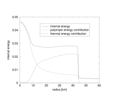
Figure 5: Radial distribution of the internal energy $\epsilon$ (solid line) shortly after bounce ($u_{B}=41$ ms) for the collapse model $\mathfrak{A}$. The different contributions from the polytropic part $\epsilon_{p}$ (dashed line) and the thermal part $\epsilon_{th}$ (long-dashed line) to the total internal energy are also shown. In front of the shock which is located at a radius of $\sim 45$ km, the thermal energy vanishes.

Correspondingly, Fig. 3 shows different snapshots of the radial velocity $u^{r}$ at evolution times close to bounce. In the inner region (the so-called homologous inner core), the infall velocity measured as function of radius is proportional to the radius. The homologous inner core shrinks with time. The outer limit of the homologous region, i.e. the sonic point, where the local sound speed has the same magnitude as the infall velocity, finally reaches a radius of less than $10$ km after about $40$ ms. At that time, the shock front forms, which moves outwards with a speed of $\sim 0.1$c initially. During its propagation it is gradually slowed down by the interaction with the infalling material in the outer region. It is worth to stress the ability of the code to resolve the steep shock front within only a few grid zones (typically three). This can be further seen in Fig. 4, where we plot the rest mass density $\rho$ at the shock front for a simulation of the collapse model $\mathfrak{C}01$.

Matter falling through the outward propagating shock is heated substantially. This can be seen in Fig. 5, where we plot the internal energy distribution $\epsilon$ in the central region shortly after bounce. The figure further shows the contribution to the internal energy from the polytropic part, Eq. (22), and the thermal part, Eq. (25). In the very central region, the polytropic contribution constitutes the dominant part. In contrast, the thermal energy dominates the total internal energy in the post-shock region for radii larger than a certain value (the shock forms off center), $\sim 13$ km in the specific situation shown in Fig. 5. We have verified that the global energy balance (see Ref. Siebel et al. (2002b) for more details) is well preserved in our simulations (maximum errors are of the order of $0.5-1\%$).

Fig. 6 shows two-dimensional contour plots illustrating the dynamics during collapse and bounce for model $\mathfrak{B}01$. For this particular simulation we used a resolution $(N_{x},N_{y})=(600,12).$ The figure displays isocontours of the rest mass density covering only the inner part of the iron core up to a radius of $30$ km at $40$ ms (i.e. at bounce; top panel), at 45 ms (when the shock has reached a radius of $\sim 140$ km; middle panel) and at 50 ms (when the shock wave is located at $r\sim 250$ km; bottom panel). The velocity vectors overlayed onto the contour plots are normalized to the maximum velocity in the displayed region. During the collapse phase until bounce at nuclear densities (upper panel), the initial aspherical contributions do not play a major role - the radial infall velocities dominate the dynamics. After bounce (middle and lower panel) the newly formed neutron star in the central region shows nonspherical oscillations, with fluid velocities up to about $2\times 10^{-3}c$. Qualitatively, the dynamics for the collapse model $\mathfrak{C}01$ is very similar to what is shown in Fig. 6 for model $\mathfrak{B}01$. However, the particular form of the non-spherical pulsations created after bounce differs.

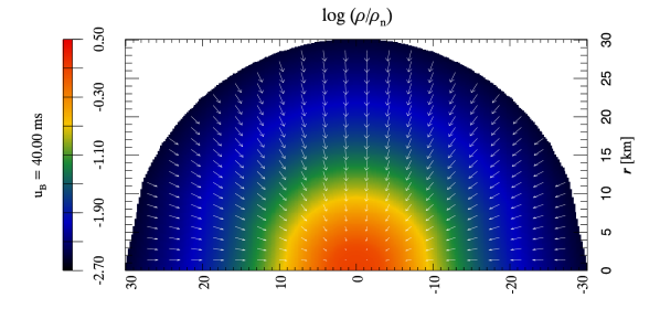
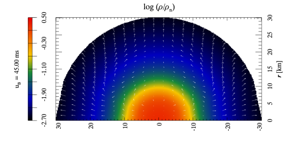
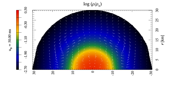
Figure 6: Contour plot of the rest mass density distribution for model $\mathfrak{B}01$ at a Bondi time $u_{B}=40$ ms (upper panel), $u_{B}=45$ ms (middle panel) and $u_{B}=50$ ms (lower panel), obtained from a global evolution extending the grid to future null infinity. We only show a fraction of the core up to a radius of $30$ km. Overlayed are velocity vectors. At bounce (upper panel), the matter distribution is, to a great extent, spherically symmetric . In the later phases (middle and lower panels), the fluid dynamics is characterized by aspherical flows related to the oscillations of the newborn neutron star. The matter flow shows reflection symmetry with respect to the equator, which is inherent to the initial data and well preserved during the evolution.

IV.2 Fluid oscillations in the outer core

When analyzing the dynamical behavior of the fluid after bounce, we find that the meridional velocity oscillates strongly in the entire pre-shock region. This can be seen from the solid curve of Fig. 7, where we plot the meridional velocity component $v_{2}=ru^{\theta}$ for model $\mathfrak{B}01$ as a function of the Bondi time, and at coordinate location $r=833$ km and $y=0.5$. These oscillations are created directly after the formation of the proto-neutron star in the central region of the numerical domain. The only possibility to propagate information instantaneously (i.e. on a slice with constant retarded time $u$) from the central region to the outer layers of the iron core is through the metric, since sound waves would need several 10 ms to cover the distance. There are two possible explanations for these oscillations. Either they are created when gravitational wave energy is absorbed well ahead of the shock, or they are created by our choice of coordinates, i.e. they are gauge effects. In the latter case, the oscillations would not be caused by a real flow, but as a consequence of the underlying coordinate system in which we describe the flow.

To clarify the origin of the oscillations we estimate in the following the kinetic energy of the oscillations, assuming that they are a physical effect. The average amplitude of the oscillation is of the order of $\hat{v}_{2}=2\times 10^{-4}c$. Note that $v_{2}$ vanishes at the polar axis and at the equator, so that the average velocity is substantially smaller than that shown in Fig. 7. Taking into account that the total mass in the pre-shock region is of the order of $M_{\mathrm{ps}}\sim 1M_{\odot}$, the kinetic energy of the oscillations is roughly

$$E_{\mathrm{kin}}\approx\frac{1}{2}M_{\mathrm{ps}}(\hat{v}_{2})^{2}\approx 2\times 10^{-8}M_{\odot}c^{2}.$$ (43)

This energy is comparable to the total energy radiated in gravitational waves in a typical core collapse event Zwerger and Müller (1997); Dimmelmeier et al. (2002a). Transferring such an amount of energy to the pre-shock region seems unphysical, as gravitational waves interact with matter only very weakly. Instead, as we describe next, we conclude that the oscillations are mainly introduced by our choice of coordinates.

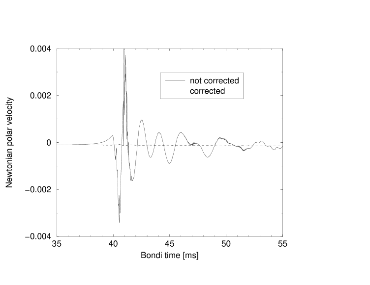
Figure 7: Meridional velocity component as a function of Bondi time at the fixed location $r=833$ km and $y=0.5$ for model $\mathfrak{B}01$. The radial location was chosen well ahead of the shock. The solid line corresponds to the meridional velocity as extracted in our coordinate system, $v_{2}=ru^{\theta}$, in units of the speed of light $c$. The dashed line corresponds to the meridional velocity evaluated in inertial Bondi coordinates defined at future null infinity. See text for more details.

Following the work of Bishop et al. Bishop et al. (1997) inertial coordinates can be established at future null infinity $\mbox{$\cal J$}^{+}$. The angular inertial coordinate $\theta_{B}$ can be constructed solving the partial differential equation

$$(\partial_{u}+U\partial_{\theta})\theta_{B}=0,$$ (44)

with initial data $\theta_{B}(u=0)=\theta(u=0)$. Instead of solving Eq. (44) directly, we determine its characteristic curves,

$$\frac{d\theta}{du} = U(\theta,u),$$ (45)

$$\theta(u=0) = \theta_{B},$$ (46)

along which $\theta_{B}$ is constant. With suitable interpolations, $\theta_{B}$ can then be determined for arbitrary angles $\theta$.

Making use of Eq. (44), it is possible to define an “inertial” meridional 4-velocity component

$$u^{\theta_{B}}=\frac{\partial\theta_{B}}{\partial\theta}\Big{|}_{u}^{\footnotesize{\mbox{$\cal J$}^{+}}}(u^{\theta}-U\Big{|}^{\footnotesize{\mbox{$\cal J$}^{+}}}u^{u}).$$ (47)

The dashed line in Fig. 7 shows the corrected (“inertial”) meridional velocity $ru^{\theta_{B}}$. Remarkably, the oscillations have almost disappeared, which clearly shows that gauge effects can play a major role for the collapse dynamics in the pre-shock region.

V Gravitational waves

V.1 Quadrupole gravitational waves

The common approach to the description of gravitational waves for a fluid system relies on the quadrupole formula Landau and Lifshitz (1961). The standard quadrupole formula is valid for weak sources of gravitational waves under the assumptions of slow motion and wave lengths of the emitted gravitational waves smaller than the typical extension of the source. The requirement that the sources of gravitational waves are weak includes the requirement that the gravitational forces inside the source can be neglected. This first approximation can be extended based on Post-Newtonian expansions (for a detailed description see the recent review Blanchet (2002) and references therein).

In a series of papers Winicour (1983, 1984); Isaacson et al. (1984); Winicour (1987), Winicour established that the quadrupole radiation formula can be derived in the Newtonian limit of the characteristic field equations. Let $Q$ be the quadrupole moment transverse to the $(\theta,\phi)$ direction

$$Q=q^{A}q^{B}\Big{(}\frac{x^{i}}{r}\Big{)}_{,A}\Big{(}\frac{x^{j}}{r}\Big{)}_{,B}Q_{ij},$$ (48)

where

$$Q_{ij}=\int\rho(x_{i}x_{j}-\delta_{ij}r^{2}/3)d^{3}x$$ (49)

is the quadrupole tensor and $q_{A}$, $A=2,3$, is the complex dyad for the unit sphere metric

$$d\theta^{2}+\sin^{2}\theta d\phi^{2}=2q_{(A}q_{B)}dx^{A}dx^{B}.$$ (50)

As usual we use parentheses to denote the symmetric part. For our axisymmetric setup, Eq. (48) reduces to

$$Q=\pi\sin^{2}\theta\int_{0}^{R}dr^{\prime}\int_{0}^{\pi}\sin\theta^{\prime}d\theta^{\prime}r^{\prime 4}\rho\Big{(}\frac{3}{2}\cos^{2}\theta^{\prime}-\frac{1}{2}\Big{)}.$$ (51)

On the level of the quadrupole approximation Winicour (1987) the quadrupole news $N_{0}$ reads

$$N_{0}=\frac{d^{3}}{du_{B}^{3}}Q.$$ (52)

With our null foliation it is natural to evaluate the quadrupole moment (51) as a function of retarded time, i.e., for the evaluation of the integral we completely relax the assumption of slow motion.

It is well known Finn (1989) that the third numerical time derivative appearing in Eq. (52) can lead to severe numerical problems resulting in numerical noise which dominates the quadrupole signal. Therefore, we make use of the fluid equations in the Newtonian limit to eliminate one time derivative. Defining the “Newtonian velocities”

$$v_{1} = u^{r}=\frac{dr}{dx}u^{x},$$ (53)

$$v_{2} = ru^{\theta}=r\frac{u^{y}}{\sin\theta},$$ (54)

the quadrupole radiation formula (52) can be rewritten with the use of the continuity equation as the so-called first moment of momentum formula

$$N_{0} = \frac{d^{2}}{du_{B}^{2}}\Big{(}\pi\sin^{2}\theta\int_{0}^{R}dr^{\prime}\int_{0}^{\pi}\sin\theta^{\prime}d\theta^{\prime}r^{\prime 3}$$ (55)

$$\times \rho(v_{1}(3\cos^{2}\theta^{\prime}-1)-3v_{2}\sin\theta^{\prime}\cos\theta^{\prime})\Big{)}.$$

We henceforth work with Eqs. (52) and (55) for estimating the quadrupole radiation. In addition, following earlier work Mönchmeyer et al. (1991); Zwerger and Müller (1997), we define the quantity $A_{20}^{E2}$, which enters the total power radiated in gravitational waves in the quadrupole approximation as

$$\frac{dE}{du_{B}}=\frac{1}{32\pi}\Big{(}\frac{dA_{20}^{E2}}{du_{B}}\Big{)}^{2}.$$ (56)

$A_{20}^{E2}$ also arises as coefficient for the quadrupolar term in the expansion of the quadrupole strain (i.e. the gravitational wave signal) $h_{+}$ in spherical harmonics note (2003)

$$h_{+}(u_{B})=\frac{1}{8}\sqrt{\frac{15}{\pi}}\sin^{2}\theta\frac{A_{20}^{E2}(u_{B})}{R},$$ (57)

where $R$ denotes the distance between the observer and the source. $A_{20}^{E2}$ can be deduced from the quadrupole moment as

$$A_{20}^{E2} = \frac{16}{\sqrt{15}}\pi^{\frac{3}{2}}\frac{d^{2}}{du_{B}^{2}}\Big{[}\int_{0}^{R}dr^{\prime}$$ (58)

$$\int_{0}^{\pi}\sin\theta^{\prime}d\theta^{\prime}r^{\prime 4}\rho\Big{(}\frac{3}{2}\cos^{2}\theta^{\prime}-\frac{1}{2}\Big{)}\Big{]},$$

or alternatively using the first moment of momentum formula in order to eliminate one time derivate, in analogy to the transition from Eq. (52) to Eq. (55), i.e.,

$$A_{20}^{E2} = \frac{16}{\sqrt{15}}\pi^{\frac{3}{2}}\frac{d}{du_{B}}\Big{[}\int_{0}^{R}dr^{\prime}\int_{0}^{\pi}\sin\theta^{\prime}d\theta^{\prime}r^{\prime 3}$$ (59)

$$\times \rho(v_{1}(3\cos^{2}\theta^{\prime}-1)-3v_{2}\sin\theta^{\prime}\cos\theta^{\prime})\Big{]}.$$

As shown in Fig. 8 we find good agreement when computing the wave strain $A_{20}^{E2}$ using Eq. (58) and Eq. (59). In order not to have the time derivatives dominated by numerical noise, we have averaged the matter contribution in the integrands of Eq. (58) and Eq. (59) over a few neighboring grid points before calculating the time derivatives.

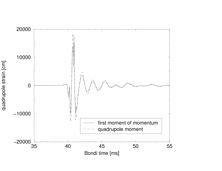
Figure 8: Gravitational wave strain $A_{20}^{E2}$ for the simulation of the collapse model $\mathfrak{B}01$. The solid curve shows the result using the first moment of momentum approach Eq. (59), the dashed line is based on Eq. (58). The good agreement found between both approaches shows that our general relativistic fluid evolution is internally consistent.

This result checks the implementation of the continuity equation and, as this equation is not calculated separately but as a part of a system of balance laws, it also checks the overall implementation of the fluid equations in the code. We note that the equivalence between Eq. (58) and Eq. (59) is only strictly valid in the Minkowskian limit and for small velocities, which is the origin for the observed small differences between the curves in Fig. 8. Substituting $\rho$ by $\rho u^{u}e^{2\beta}$ in Eq. (58) and by $\rho e^{2\beta}$ in Eq. (59), by which we restore the equivalence in a general relativistic spacetime, we find excellent agreement between the two approaches for calculating $A_{20}^{E2}$.

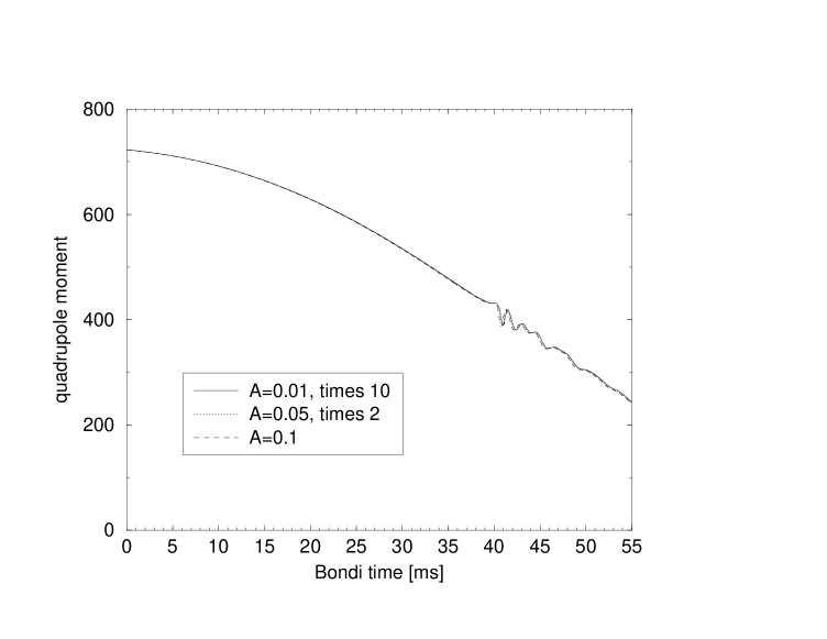
Figure 9: Quadrupole moment Q (in units $c=G=M_{\odot}=1$) as a function of time for three models of type $\mathfrak{B}$ with perturbation amplitude $A=0.01$, $A=0.05$ and $A=0.1$. The first two results are rescaled with respect to $A=0.1$ assuming a linear dependence. All three curves overlap in the diagram. The quadrupole moment (and hence the quadrupole signal) scales linearly with the amplitude of the perturbation in the chosen parameter region.

Since we are imposing only small perturbations from spherical symmetry, we expect a linear dependence of the non-spherical dynamics and the gravitational wave signal as a function of the perturbation amplitude. We have verified in a series of runs that the amplitude of the quadrupole moment (and thus the quadrupole radiation signal) indeed scales linearly with the amplitude of the initial perturbations (see Fig. 9). This observation marks another important test for the correctness of the global dynamics of our code.

On the other hand, when comparing the quadrupole news defined in Eq. (52) or Eq. (55) with the Bondi news signal $N$ evaluated at future null infinity (which is defined in Eq. (68) below), we find important discrepancies. This can be seen in Fig. 10, where we plot both, the Bondi news and the quadrupole news for model $\mathfrak{B}01$. We note that the differences manifest themselves not only in the amplitude of the oscillations, but also in the frequencies of the signals. This behavior is clearly different from the one we observed in the studies of neutron star pulsation carried out in Ref. Siebel et al. (2002b), where both signals showed very good agreement.

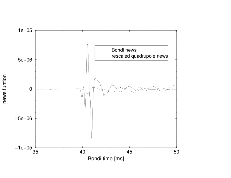
Figure 10: Bondi and quadrupole news as a function of time for model $\mathfrak{B}01$. The solid curve corresponds to the quadrupole news according to Eq. (55), the dashed curve to the Bondi news signal. For visualization reasons, we have divided the quadrupole news result by 50. Remarkable disagreement is found between both signals.

As mentioned above, the quadrupole formula is only the first term in a Post-Newtonian expansion for the gravitational radiation. The next, non-vanishing contribution to the gravitational strain for our axisymmetric configuration is the hexadecapole contribution, which reads Mönchmeyer et al. (1991)

$$h_{+}^{HD}=\frac{9}{8}\sqrt{\frac{5}{\pi}}\sin^{2}\theta(1-\frac{7}{6}\sin^{2}\theta)\frac{A_{40}^{E2}}{R}.$$ (60)

The quantity $A_{40}^{E2}$ is defined as

$$A_{40}^{E2} = \frac{d^{4}}{du_{B}^{4}}M_{40}^{E2},$$ (61)

$$M_{40}^{E2} = \frac{\sqrt{5}}{63}\pi^{\frac{3}{2}}\int_{0}^{R}dr^{\prime}\int_{0}^{\pi}\sin\theta^{\prime}d\theta^{\prime}r^{\prime 6}$$ (62)

$$\times \rho(7\cos^{4}\theta^{\prime}-6\cos^{2}\theta^{\prime}+\frac{3}{5}),$$

or alternatively

$$A_{40}^{E2} = \frac{d^{3}}{du_{B}^{3}}N_{40}^{E2},$$ (63)

$$N_{40}^{E2} = \frac{4\sqrt{5}}{63}\pi^{\frac{3}{2}}\int_{0}^{R}dr^{\prime}\int_{0}^{\pi}\sin\theta^{\prime}d\theta^{\prime}r^{\prime 5}$$ (64)

$$\times \rho\Big{(}v_{1}(7\cos^{4}\theta^{\prime}-6\cos^{2}\theta^{\prime}+\frac{3}{5})$$

$$+v_{2}(3-7\cos^{2}\theta^{\prime})\sin\theta^{\prime}\cos\theta^{\prime}\Big{)}.$$

By extracting the hexadecapole moment for the above result, we found, however, that the associated amplitude is too small in order to explain the observed differences in Fig. 10. In addition, one would expect in general that the contribution of the hexadecapole moment increases the amplitude of the approximate signal. However, the amplitude of the quadrupole news in Fig. 10 is already much larger than that of the Bondi news evaluated at $\mbox{$\cal J$}^{+}$.

As we discussed in the preceding section, the global dynamics of the core collapse and bounce is correctly reproduced with our numerical code (see also the validation tests in the Appendix). We have strong evidence that the quadrupole signals extracted from our collapse simulations do not correspond to physical gravitational wave signals. In the following, we describe the different arguments which support this claim.

First, if the quadrupole radiation signal corresponded to the true physical signal, it would be very difficult to understand why the Bondi signal has a significantly smaller amplitude. In the calculation of the Bondi news, Eq. (68), the contribution of the different terms are relatively large and add up to a small signal (see below). Under the assumption that the quadrupole news signal is correct and the Bondi news signal is wrong, it is extremely unlikely that possible errors in the contribution to the Bondi news add up to a very small signal.

Second, we have performed comparisons between our numerical code and the code of Refs. Dimmelmeier et al. (2002b, a), finding much larger amplitudes for the quadrupole gravitational wave signal in our case. However, we note that comparing the results of both codes in axisymmetry is ambiguous, as possible differences might have different explanations. For example, the use of the conformally flat metric approach in Dimmelmeier et al. (2002b, a) is clearly an approximation to general relativity, which should create some differences. Furthermore, the coordinate systems used in both codes for the computation of the quadrupole moment are different. Only in our code, the quadrupole moment is evaluated on a light cone, i.e. as a function of retarded time.

Figure 11: Radial contribution to the quadrupole moment. We plot the value of the integral $Q(r)=\pi\sin^{2}\theta\int_{0}^{r}dr^{\prime}\int_{0}^{\pi}\sin\theta^{\prime}d\theta^{\prime}r^{\prime 4}\rho(\frac{3}{2}\cos^{2}\theta^{\prime}-\frac{1}{2})$ as a function of the radial coordinate $r$ for different values of time. The data is plotted after a fixed number of time steps, starting with initial data at $u_{B}=0$ ms (upper solid curve). The data was taken from a simulation of model $\mathfrak{B}01$. Large amplitude oscillations of the quadrupole moment, as they can be seen in Fig. 9, can only be created - at least shortly after bounce - in the outer region of the infalling matter well in front of the shock.

A third and physically motivated argument stems from the spatial distribution of matter in our simulation. As it can be seen from Fig. 11, the main contribution to the radial integral of the quadrupole moment comes from the outer, infalling layers of matter. These outer layers are responsible for the oscillations in the quadrupole moment, which can be seen in Fig. 9. Following the same reasoning as in the previous section it is obvious to conclude that the calculation of the quadrupole moment is also affected by our choice of coordinates, i.e. by gauge effects.

For all these reasons we extract the quadrupole moment in the angular coordinate system defined by Eq. (44). However, introducing the inertial angular coordinate does not help to obtain a better agreement between quadrupole and Bondi signals, the extracted quadrupole moment almost agrees with the results shown in Fig. 9. Since the difference of Bondi time between the different angular directions on our Tamburino-Winicour foliation is in general of the same order as the lapse of time for one time step, we expect a similar result when evaluating the quadrupole moment at a fixed inertial time. However, by prescribing the necessary coordinate transformations to define Bondi coordinates only at $\mbox{$\cal J$}^{+}$, we do not take into account an inertial radial coordinate, which should be used for the evaluation of the quadrupole moment.

As already mentioned before, in Ref. Siebel et al. (2002b) we found good agreement between the Bondi signal and the quadrupole signal when calculating gravitational waves from pulsating relativistic stars. Hence, the obvious question arises of why the quadrupole formula could be applied in those scenarios. The answer lies in the small velocities encountered in the problem of neutron star pulsations. Whereas the typical maximum fluid velocities in the oscillation problem are of the order of $10^{-5}c-10^{-4}c$, fluid velocities of up to $0.2c$ are reached for the core collapse scenario. Furthermore, due to the non-spherical dynamics of the proto-neutron star formed in the interior of the collapsed region, the metric can pick up gauge contributions which are created as a consequence of our requirement to prescribe a local Minkowski frame at the vertex of the light cones. Gauge contributions may also play a more important role in the collapse scenario due to the enlarged radial extension of the collapsing iron core (about 1500 km), which is much larger than the corresponding one for neutron star pulsations (about 15 km).

We note that since the collapse involves fluid velocities of up to $0.2c$, it is not obvious whether the functional form for the quadrupole moment established in the slow motion limit on the light cone will still be valid. In fact, the situation could be similar to the case of the total mass of spacetime, where a naive definition, even in spherical symmetry, as

$$M_{n}=4\pi\int_{0}^{R}r^{\prime 2}\rho(1+\epsilon)dr^{\prime},$$ (65)

would only be a valid approximation for small fluid velocities. This can be understood from the comparison with the expression of the Bondi mass in the form

$$M_{B}=4\pi\int_{0}^{R}r^{\prime 2}[\rho(1+\epsilon)(-u^{u}u_{u})-p(1+u^{u}u_{u})]dr^{\prime},$$ (66)

(no summation is involved in this expression). Only vanishing fluid velocities, i.e. $u^{u}u_{u}=-1$, ensure that the two masses are equal, $M_{n}=M_{B}$.

We experimented with possible alternative functional forms for the quadrupole moment which result in significant differences. An unambiguous clarification of which functional form has to be used for the quadrupole moment in the extended regime of validity of large fluid velocities could only be obtained by a derivation of the quadrupole formula in the Tamburino gauge. However, technical complications for such a derivation are so severe that it has only been accomplished for a simplified radiating dust model Isaacson et al. (1983) (see the related discussion in Ref. Winicour (1987)).

V.2 The Bondi news signal

The numerical extraction of the Bondi news is a very complicated undertaking. Reasons for possible numerical problems are diverse: First, its extraction involves calculating non-leading terms from the metric expansion at future null infinity. All the metric quantities are global quantities, and are thus sensitive to any numerical problem in the entire computational domain. Second, when calculating the gravitational signal in the Tamburino-Winicour approach, one has to take into account gauge effects. For the present calculations of the gravitational wave signal from core collapse, the gauge contributions are indeed the dominant contribution, which can easily influence the physical signal.

We have described in detail the formalism and numerical methods to deal with gravitational waves without approximation in our axisymmetric characteristic code in Ref. Siebel et al. (2002b). In the following, we will only repeat the most important aspects. The total energy emitted by gravitational waves to infinity during the time interval $[u,u+du]$ in the angular direction $[y,y+dy]$ is given by the expression

$$dE=\frac{1}{2}N^{2}\omega^{3}e^{2H}dydu,$$ (67)

where the Bondi news function $N$ reads

$$N = \frac{1}{2}\frac{e^{-2H}}{\omega^{2}}\left\{2c_{,u}+\frac{(\sin\theta\ c^{2}\ L),_{\theta}}{\sin\theta\ c}\right.$$ (68)

$$\left.+e^{-2K}\omega\sin\theta[\frac{(e^{2H}\omega)_{,\theta}}{\omega^{2}\sin\theta}]_{,\theta}\right\}.$$

$K,c,H$ and $L$ are defined by a power series expansion of the metric quantities at $\mbox{$\cal J$}^{+}$ as follows,

$$\gamma = K+\frac{c}{r}+O(r^{-2}),$$ (69)

$$\beta = H+O(r^{-2}),$$ (70)

$$U = L+O(r^{-1}).$$ (71)

Figure 12: Different contributions to the Bondi news. The solid curve corresponds to the term involving $c_{u}$ (first addend) in Eq. (68), the dashed curve to the contribution from the second and third addend. By summing up both contributions we obtain the Bondi news, which is close to zero. In addition, we note that when separating the third addend into angular derivatives of $H$ and $\omega$, each single contribution has an amplitude 23 times larger than what is shown in the figure.

We plot in Fig. 12 the different contributions to the Bondi news for the collapse model $\mathfrak{B}01$. It becomes clear from this plot that a very accurate determination of the metric fields is essential. As it can be further seen in this figure, the metric quantities show high frequency numerical noise, as soon as the shock forms (at a Bondi time of about $40$ ms). In order to demonstrate that the noise is actually created at the shock, we plot in Fig. 13 the location of the shock together with the gravitational wave signal. Clearly, the noise is created by the motion of the shock across the grid, its temporal behavior following the discontinuous jumps of the shock between adjacent grid cells. We note that due to the coarser radial resolution used in the outer layers of the core, the frequency of the noise slowly decreases with time.

Figure 13: Upper panel: Bondi news as a function of time. High frequency noise is overlayed on top of a small frequency modulation. Lower panel: Time evolution of the radial location of the cross section of the shock front with the equator. Due to the finite resolution, the location of the shock wave moves discontinuously. The frequency of these jumps coincides with that of the noise in the Bondi news. Once created at the shock, the noise is propagated instantaneously to infinity through the numerical solution of the metric equations.

As we have pointed out in the previous section, the shock front is well captured in only a few radial zones with our high-resolution shock-capturing scheme. It might seem surprising that a small localized error created in a few radial zones can have such a large effect on the gravitational wave signal. However, one has to keep in mind that the radial integration of the metric variables picks up this error and propagates it to future null infinity instantaneously. It is important to stress that the effect of the numerical noise on the dynamics of the collapse and bounce is entirely negligible. However, the extraction of the Bondi news signal is extremely sensitive to it.

We have verified that the frequency of the noise increases, as expected, with radial resolution. Unfortunately, its amplitude does not decrease substantially with radial resolution, at least not in the resolution regime accessible to us note (2003). Therefore, we tried to eliminate the noise by different methods. In a first attempt, we smoothed out the shock front, either in the hydrodynamical evolution itself or before using the fluid variables in the source terms of the metric equations. In both cases, it was impossible to obtain a smooth signal without changing the dynamics. In a second attempt, following the work of Gómez (2001), we rearranged the metric equations eliminating second derivatives which might be ill-behaved at the shock. Defining a metric quantity

$$X=r^{2}f^{2}e^{2(\gamma-\beta)}\hat{U}_{,x}-2(\beta_{,y}-(1-y^{2})\hat{\gamma}_{,y}),$$ (72)

and solving the hypersurface equations successively for $\beta$, $X$, $\hat{U}$ and $S$, it is possible to eliminate all second derivatives from the hypersurface equations. Unfortunately, the noise is not significantly reduced by this rearrangement of the metric equations. Finally, going to larger time steps for the fluid evolution only - solving the metric equations several times between one fluid time step - was not effective either.

Figure 14: Bondi news as a function of Bondi time for the collapse model $\mathfrak{B}01$. The displayed time interval covers the late collapse stage until several ms after bounce at about $t=40$ ms. During the collapse stage, the gravitational wave signal is negligible. After bounce a complicated series of oscillations sets in.

After these attempts we decided to eliminate the noise from the gravitational wave signals only after the numerical evolution. We experimented with two different smoothing methods. In the first method, we calculate the Fourier transform of the data, and eliminate all frequencies beyond a certain threshold frequency (of about 5 - 10 kHz). Then, when transforming back from Fourier space all the high-frequency part of the data is removed. In a second method we simply average the signal over a few neighboring points. We have applied this second method in what is described below.

Fig. 14 shows the Bondi news signal for the collapse model $\mathfrak{B}01$. The figure focuses on the part of the signal around bounce. After the initial gravitational wave content is radiated away (in the first $5$ ms, not depicted in the figure), the signal in the collapse stage is very weak. This is expected, as the dynamics is well reproduced by a spherical collapse model during this stage. At bounce, the Bondi news shows a spike. Afterwards, a complicated series of oscillations is created due to the pulsations of the forming neutron star and the outward propagation of the shock. Typical oscillation frequencies are of the order of $0.5-1$ kHz, at which the current gravitational wave laser interferometers have maximum sensitivity.

Correspondingly, Fig. 15 shows the Bondi news signal for the collapse model $\mathfrak{C}01$. Here again, after radiating away the initial gravitational wave content, the collapse phase is characterized by very small radiation of gravitational waves. At bounce, we again observe a strong spike in the signal. Afterwards, the oscillations in the signal are rather rapidly damped.

Figure 15: Bondi news as a function of time for the collapse model $\mathfrak{C}01$. The bounce at about 41 ms is characterized by a large spike in the gravitational wave signal. After bounce, the signal shows oscillations, with a principal frequency of about $0.35$ kHz.

We stress that as a consequence of the necessary smoothing techniques applied, only the main features of the gravitational wave signals in Figs. 14 and 15 are reliably reproduced. This also applies to possible offsets of the Bondi news, which affect in particular the gravitational wave strain. Comparing the Bondi news function for the different collapse models of type $\mathfrak{B}$, we observe to good approximation a linear dependence of the Bondi news with the perturbation amplitude. This is reflected in the total energy radiated away in gravitational waves, which scales quadratically with the amplitude of the initial perturbation. A summary of the results on the gravitational wave energy is listed in in Table 1.

Table 1: Total energy radiated in gravitational waves during the first 50 ms for the collapse simulations of type $\mathfrak{B}$. The initial gravitational wave content is the dominant contribution to the total energy. This energy scales quadratically with the amplitude of the initial perturbation, as can be inferred from the last column, where the corresponding energies have been rescaled with respect to that of collapse model $\mathfrak{B}01$.

model	total energy radiated [$M_{\odot}$]	rescaled result [$M_{\odot}$]
$\mathfrak{B}001$	$4.31\times 10^{-9}$	$4.31\times 10^{-7}$
$\mathfrak{B}005$	$1.08\times 10^{-7}$	$4.32\times 10^{-7}$
$\mathfrak{B}01$	$4.32\times 10^{-7}$	$4.32\times 10^{-7}$

VI Discussion

We have presented first results from axisymmetric core collapse simulations in general relativity. Contrary to traditional approaches, our framework uses a foliation based on a family of light cones, emanating from a regular center, and terminating at future null infinity. To the best of our knowledge, the characteristic formulation of general relativity has never been used before in simulations of supernova core collapse and in the extraction of the associated exact gravitational waves. Our axisymmetric hydrodynamics code is accurate enough to allow for a detailed analysis of the global dynamics of core collapse in general. But we have not found a robust method for the (Bondi news) gravitational wave extraction in the presence of strong shock waves.

Comparing our results to other recent work on relativistic supernova core collapse Dimmelmeier et al. (2001); Dimmelmeier et al. (2002a), it is not surprising that numerical noise in the gravitational waveforms is more noticeable in our approach. Whereas in the conformal flat metric approach employed in Dimmelmeier et al. (2001); Dimmelmeier et al. (2002a) the metric equations of general relativity reduce to elliptic equations, which naturally smooth out high-frequency numerical noise, we solve for the gravitational wave degrees of freedom directly using the full set of field equations of general relativity, and hence we have to solve a hyperbolic equation. It remains to be seen whether a similar numerical noise to the one we find when extracting the gravitational wave signal will be encountered in core collapse simulations solving the full set of Einstein equations in the Cauchy approach. In this respect we mention recent axisymmetric simulations by Shibata using a conformal-traceless reformulation of the ADM system Shibata (2002) where, despite of the fact that long-term rotational collapse simulations could be accurately performed, gravitational waves could not be extracted from the raw numerical data since their amplitude is much smaller than that of other components contained in the metric and/or numerical noise.

With the current analysis we have presented in this paper, it is not obvious how the numerical noise of the Bondi news can be effectively eliminated. Including rotation in the simulations, which would be the natural next step for a more realistic description of the scenario, could help in this respect. Due to the global asphericities introduced by rotation, one would expect, in general, gravitational wave signals of larger amplitude, which could make the numerical noise less important, if not completely irrelevant. In addition to this possibility we propose the following methods to improve the extraction of the gravitational wave signals: In a first approach one should try to rearrange the metric equations by introducing auxiliary fields which could effectively help to diminish the importance of high-order derivatives, especially of the fluid variables, which can be discontinuous. Unfortunately, to the best of our knowledge, there is no clear guideline to what is really needed to eliminate the numerical noise completely, apart from the hints given by Gómez (2001). Our attempts in this direction have not yet been successful, but we believe there is still room for improvement. Alternatively, one should try to implement pseudospectral methods for the metric update. Pseudospectral methods would allow for a more efficient and accurate numerical solution of the metric equations. In a third promising line of research we propose to consider the inclusion of adaptive grids and methods of shock fitting into the current code. With the help of an adaptive grid, one could try to arrange the entire core collapse simulation in such a way that the shock front always stays at a fixed location of the numerical grid. By avoiding the motion of the shock front across the grid, one would expect the noise in the gravitational wave signals to disappear. But already increasing the radial resolution substantially in the neighborhood of the shock front could help to obtain an improved representation of the shock. All these issues are ripe for upcoming investigations.

VII Acknowledgements

It is a pleasure to thank Harald Dimmelmeier for helpful discussions and for performing reference runs with his numerical code. We further thank Masaru Shibata for comments. Our work has been supported in part by the EU Programme ’Improving the Human Research Potential and the Socio-Economic Knowledge Base’, (Research Training Network Contract HPRN-CT-2000-00137). P.P. acknowledges support from the Nuffield Foundation (award NAL/00405/G). J.A.F acknowledges support from a Marie Curie fellowship from the European Union (HPMF-CT-2001-01172) and from the Spanish Ministerio de Ciencia y Tecnología (grant AYA 2001-3490-C02-01).

Appendix A

In this Appendix we present tests specifically aimed to calibrate our code in core collapse simulations. The reader is addressed to Ref. Siebel et al. (2002b) for information on further tests the code has successfully passed concerning, among others, long-term evolutions of relativistic stars and mode-frequency calculations of pulsating relativistic stars.

A.1 Shock reflection test

In order to assess the shock-capturing properties of the code, we have performed a shock reflection test in Minkowski spacetime. This is a standard problem to calibrate hydrodynamical codes Marti and Müller (1999). A cold, relativistically inflowing ideal gas is reflected at the origin of the coordinate system, which causes the formation of a strong shock. We start the simulation with a constant density region, where $\rho=\rho_{0}$, $u^{r}=u^{r}_{\mathrm{R}}$ and $\epsilon=\epsilon_{\mathrm{R}}=0$ (we set $\epsilon\approx 10^{-11}$ for numerical reasons). From the continuity equation it follows that the rest mass density in the unshocked region obeys

$$\rho_{\mathrm{R}}(u,r)=\rho_{0}\left(1-\frac{u^{r}_{\mathrm{R}}}{u^{u}_{\mathrm{R}}r}u\right)^{2}.$$ (73)

From momentum conservation arguments, it is clear that the velocity in the shocked region vanishes, $u^{r}_{\mathrm{L}}=0$. Evaluating the Rankine-Hugoniot jump conditions for the fluid equations, we obtain:

$$s = \frac{(\Gamma-1)\epsilon_{\mathrm{L}}}{u^{u}_{\mathrm{R}}-1-\Gamma\epsilon_{\mathrm{L}}},$$ (74)

$$\epsilon_{\mathrm{L}} = u^{u}_{\mathrm{R}}+u^{r}_{\mathrm{R}}-1,$$ (75)

$$\rho_{\mathrm{L}} = \rho_{s}\frac{\Gamma(u^{r}_{\mathrm{R}})^{2}-(\Gamma-1)\epsilon_{\mathrm{L}}}{(\Gamma-1)\epsilon_{\mathrm{L}}},$$ (76)

$$p_{\mathrm{L}} = (\Gamma-1)\rho_{\mathrm{L}}\epsilon_{\mathrm{L}}.$$ (77)

Here, $s$ denotes the shock speed and $\rho_{s}=\rho_{\mathrm{R}}(u,r=su)$ the rest mass density in front of the shock.

We performed this test with different values of the fluid velocity, and different schemes for the fluid evolution. Fig. 16 shows the results for an ultrarelativistic flow ($u^{r}=-0.9999c$). For this particular test we used the HLL solver and increased the numerical viscosity by a factor 2 in order to damp small post-shock oscillations. The agreement with the analytic solution is satisfactory, and the shock front is very steep, being resolved with only one or two radial zones. The deviation close to the origin is a well-known failure of finite-difference schemes for this problem (see, e.g. Noh (1987)), which is not important for our purposes.

Figure 16: Shock reflection test for an ultrarelativistic flow with $u^{r}=-0.9999$c and $\rho_{0}=8$ and EoS $p=5\times 10^{-4}\rho^{\frac{5}{3}}$, which is reflected at the origin of the coordinate system. We have plotted different fluid quantities at an evolution time $u=2.029$ as a function of the radial coordinate $r$. Top panel: fluid velocity $u^{r}$. Middle Panel: pressure $p$. Bottom Panel: rest mass density $\rho$. The solid line corresponds to the exact solution, the crosses are taken from our numerical simulation. For the above result, we made use of a non-equidistant radial grid $r=x/(1-x^{\frac{5}{2}})$ with 800 radial zones, the MC slope limiter and the HLL approximate Riemann solver.

A.2 Convergence tests

We describe now some tests which check various properties of spherically-symmetric core collapse. We choose a particular collapse model, for which the initial central density is $\rho_{c}=1.62\times 10^{-8}$ (in units $G=c=M_{\odot}=1$), the polytropic constant is $\kappa=0.46$, and the collapse is induced by resetting the adiabatic exponent to $\Gamma_{1}=1.3$ (for the equilibrium model with $\Gamma=\frac{4}{3}$). We use the hybrid EoS discussed in Section II.3.

A.2.1 Thermal energy during the infall phase

Before the central density of the collapsing core reaches nuclear densities, the collapse is exactly adiabatic. Hence, the thermal energy, which vanishes initially, should vanish throughout this phase. This can be easily checked and used for convergence tests. Fig. 17 shows the result after an integration time of $30$ ms (when the central density has increased by roughly a factor 10). We find that the errors from the exact result $\epsilon_{\mathrm{th}}=0$ converge to zero, the convergence rate is 2. Note that although $\epsilon_{th}\geq 0$ from the physical point of view, the numerical errors can result in negative values for $\epsilon_{\mathrm{th}}$.

Figure 17: Thermal energy as a function of the radial coordinate $x$ at $30$ ms for a compactified grid $r=\frac{200x}{1-x^{2}}$ for different resolutions. Due to numerical errors, the thermal energy is different from zero. Deviations converge to zero, the convergence rate is 2.

A.2.2 Time of bounce

Using the axisymmetric code developed by Dimmelmeier et al. Dimmelmeier et al. (2001); Dimmelmeier et al. (2002b, a) based on the conformally flat metric approach, we can perform comparisons between the evolutions of the same initial models. As the conformally flat metric approximation is exact for spherical models, comparisons in spherical symmetry are unambiguous.

Figure 18: Evolution of the central density for a core collapse induced by resetting the adiabatic exponent to $\Gamma_{1}=1.30$. The central density increases by almost 5 orders of magnitude, before the core bounces. Afterwards the central density stays almost constant. The different lines correspond to different grid functions and resolutions, see run 4, 1 and 5 in Table 2.

We define the time of bounce as the time, when the central density reaches its maximum. In order to start with the same initial data we initiate the collapse by ray-tracing the evolution of Dimmelmeier’s code to obtain the initial data on our null cone. There is no principal advantage in starting with initial data on a null cone or on a Cauchy slice. Ideally, results from stellar evolution would give exact initial conditions for the core collapse, thus eliminating the artificial procedure of resetting $\Gamma$ to initiate the collapse. Fig. 18 shows the evolution of the central density for the relativistic code of Dimmelmeier et al. (2002b) and the results of our null code for two different grid functions. Table 2 summarizes our results for the time of bounce.

Assuming our code is exactly second order convergent and extrapolating our results to an hypothetical infinite resolution, we obtain from runs 3 and 4, that the infinite resolution run bounces after $38.65$ ms. This is internally consistent, a comparison of runs 2 and 4 results in a value of $38.66$ ms. Using an even higher resolution for a different grid function in run 5, we observe a time of bounce close to the converged result. Our results on the time of bounce are in very good agreement with the result of Dimmelmeier et al. (2002b), who find a value of $38.32$ ms. The observed difference of less than $1\%$ is either due to the fact that the result of Dimmelmeier et al. (2002b) is not converged, or due to the different radial coordinates used in both codes, and thus small differences in the initial data.

Table 2: Times of bounce for different grid functions and resolutions.

	code	grid	radial	time of
		function	resolution	bounce [ms]
1	CFC code Dimmelmeier et al. (2002b)	see  Dimmelmeier et al. (2002b)	$80^{*}$	38.32
2	null code	$r=\frac{150x}{1-x^{4}}$	600	40.86
3	null code	$r=\frac{150x}{1-x^{4}}$	800	39.90
4	null code	$r=\frac{150x}{1-x^{4}}$	1000	39.45
5	null code	$r=100\tan(\frac{\pi}{2}x)$	1200	38.92

^∗ This number for the radial resolution cannot be directly compared to the values of our code, as we resolve the exterior vacuum region up to future null infinity with our code as well.

As it can be seen in Fig. 18, the comparison does not only give very good agreement for the time of bounce, but also for the dynamics of the central density in general. This is very important, since it shows that the global dynamics of the core collapse is correctly described in our numerical implementation.

References

- Müller (1982) E. Müller, Astron. Astrophys. 114, 53 (1982).
- Mönchmeyer et al. (1991) R. Mönchmeyer, G. Schäfer, E. Müller, and R. E. Kates, Astron. Astrophys. 246, 417 (1991).
- Zwerger and Müller (1997) T. Zwerger and E. Müller, Astron. Astrophys. 320, 209 (1997).
- Dimmelmeier et al. (2002a) H. Dimmelmeier, J. A. Font, and E. Müller, Astron. Astrophys. 393, 523 (2002a).
- Müller (1998) E. Müller, in Saas-Fee Advanced Course 27: Computational Methods for Astrophysical Fluid Flow (1998), pp. 343+.
- Yamada and Sato (1994) S. Yamada and K. Sato, Astrophys. J. 434, 268 (1994).
- Dimmelmeier et al. (2001) H. Dimmelmeier, J. A. Font, and E. Müller, Astrophy. J. Lett. 560, L163 (2001).
- Dimmelmeier et al. (2002b) H. Dimmelmeier, J. A. Font, and E. Müller, Astron. Astrophys. 388, 917 (2002b).
- Winicour (2001) J. Winicour, Liv. Rev. Relativ. 4, 3 (2001).
- Bishop et al. (1997) N. T. Bishop, R. Gómez, L. Lehner, M. Maharaj, and J. Winicour, Phys. Rev. D 56, 6298 (1997).
- Gómez et al. (1998) R. Gómez, L. Lehner, R. L. Marsa, Winicour, and et al., Phys. Rev. Lett. 80, 3915 (1998).
- Gómez et al. (1994) R. Gómez, P. Papadopoulos, and J. Winicour, J. Math. Phys. 35, 4184 (1994).
- Papadopoulos and Font (2000) P. Papadopoulos and J. A. Font, Phys. Rev. D 61, 024015+ (2000).
- Papadopoulos and Font (1999a) P. Papadopoulos and J. A. Font, gr-qc/9912094 (1999a).
- Font (2000) J. A. Font, Liv. Rev. Relativ. 3, 2 (2000).
- Papadopoulos and Font (1999b) P. Papadopoulos and J. A. Font, Phys. Rev. D 59, 044014+ (1999b).
- Siebel et al. (2002a) F. Siebel, J. A. Font, and P. Papadopoulos, Phys. Rev. D 65, 24021+ (2002a).
- Siebel et al. (2002b) F. Siebel, J. A. Font, E. Müller, and P. Papadopoulos, Phys. Rev. D 65, 64038+ (2002b).
- Bondi et al. (1962) H. Bondi, M. G. J. van der Burg, and A. W. K. Metzner, Proceedings of the Royal Society A 269, 21 (1962).
- Harten et al. (1983) A. Harten, P. D. Lax, and B. van Leer, SIAM Review 25, 35 (1983).
- van Leer (1977) B. J. van Leer, J. Comp. Phys. 23, 276 (1977).
- Font et al. (2002) J. A. Font, T. Goodale, S. Iyer, M. Miller, L. Rezzolla, E. Seidel, N. Stergioulas, W. Suen, and M. Tobias, Phys. Rev. D 65, 84024+ (2002).
- Janka et al. (1993) H.-T. Janka, T. Zwerger, and R. Mönchmeyer, Astron. Astrophys. 268, 360 (1993).
- Rampp et al. (1998) M. Rampp, E. Müller, and M. Ruffert, Astron. Astrophys. 332, 969 (1998).
- Bazan and Arnett (1994) G. Bazan and D. Arnett, Astrophy. J. Lett. 433, L41 (1994).
- note (2003) We use this term loosely, without claiming that we model the microphysics realistically.
- Landau and Lifshitz (1961) L. Landau and E. Lifshitz, The classical theory of fields (Addison-Wesley, New York, 1961).
- Blanchet (2002) L. Blanchet, Liv. Rev. Relativ. 5, 3 (2002).
- Winicour (1983) J. Winicour, J. Math. Phys. 24, 1193 (1983).
- Winicour (1984) J. Winicour, J. Math. Phys. 25, 2506 (1984).
- Isaacson et al. (1984) R. A. Isaacson, J. S. Welling, and J. Winicour, Phys. Rev. Lett. 53, 1870 (1984).
- Winicour (1987) J. Winicour, General relativity and gravitation 19, 281 (1987).
- Finn (1989) L. S. Finn, in Frontiers in numerical relativity (Cambridge University Press, Cambridge, 1989), pp. 126–145.
- note (2003) Our notation follows the work Mönchmeyer et al. (1991). denotes the electric part, denotes the , quadrupolar part in an expansion of the gravitational wave strain in tensor harmonics.
- Isaacson et al. (1983) R. A. Isaacson, J. S. Welling, and J. Winicour, J. Math. Phys. 24, 1824 (1983).
- note (2003) For a resolution , one time step is accomplished in about 2 s of CPU time on the DEC-Alpha workstations where we run the simulations achieving a performance of several hundred MFlops. Taking into account that about time steps are needed to cover the evolution up to ms for this given resolution, one single simulation takes about 16 days.
- Gómez (2001) R. Gómez, Phys. Rev. D 64, 24007+ (2001).
- Shibata (2002) M. Shibata, Phys. Rev. D, to appear (2003), gr-qc/0301103.
- Marti and Müller (1999) J. M. Marti and E. Müller, Liv. Rev. Relativ. 2, 3 (1999).
- Noh (1987) W. F. Noh, J. Comp. Phys. 72, 78 (1987).