Some properties of a $\Delta-$string

Abstract

The properties of 5D gravitational flux tubes are considered. With the cross section and 5th dimension in the Planck region such tubes can be considered as string-like objects, namely $\Delta-$strings. A model of attachment of $\Delta-$string to a spacetime is offered. It is shown that the attachment point is a model of an electric charge for an observer living in the spacetime. Magnetic charges are forbidden in this model.

Dept. Phys. and Microel. Engineer., KRSU, Bishkek,
Kievskaya Str. 44, 720000, Kyrgyz Republic

1 Introduction

Recently [1] it was assumed that some kind of gravitational flux tube solutions in the 5D Kaluza-Klein gravity can be considered as string-like objects, namely $\Delta-$strings. The idea is that the gravitational flux tubes can be very thin (approximately $\approx l_{Pl}$) and arbitrary long. Evidently that such object looks like to a string attached to two Universes or to remote parts of a single Universe. The thickness of this object is so small that near to the point of attachment to an external Universe the handles of a spacetime foam will appear between this object and the Universe. This is like a delta of the river flowing into the sea. We call such objects as a $\Delta-$string. The $\Delta-$string has interesting properties : it can transfer electromagnetic waves and consequently the energy; the mouth is similar to a spread charge; it is a realization of Einstein-Wheeler’s idea about “mass without mass” and “charge without charge”; it has wormhole and string properties; in some sense it is some realization of Einstein’s idea that all should be constructed from vacuum (in this case the $\Delta-$string is the vacuum solution of 5D gravitational equations).

At first these gravitational flux tubes solutions were obtained as 4D Levi-Civita - Robertson - Bertotti solutions [2] in 4D Einstein-Maxwell theory. It is an infinite flux tube filled with parallel electric $F_{01}$ and and magnetic $F_{23}$ fields

$$ds^{2} = a^{2}\left(\cosh^{2}\zeta dt^{2}-d\zeta^{2}-d\theta^{2}-\sin^{2}\theta d\varphi^{2}\right),$$ (1)

$$F_{01} = \rho^{1/2}\cos\alpha,\;\;\;\;\;\;\;F_{23}=\rho^{1/2}\sin\alpha,$$ (2)

where

$$G^{1/2}a\rho^{1/2}=1.$$ (3)

$\alpha$ is an arbitrary constant angle; $a$ and $\rho$ are constants defined by Eq. (3); $a$ determines the cross section of the tube and $\rho$ the magnitude of the electric and magnetic fields; $G$ is Newton’s constant ($c=1$, the speed of light); $F_{\mu\nu}$ is the electromagnetic field tensor. For $\cos\alpha=1$ ($\sin\alpha=1$) one has a purely electric (or magnetic) field.

In Ref. [3] was obtained similar 5D solutions. The properties of these solutions depend on the relation $\delta_{EH}=1-E/H$ between electric $E$ and magnetic $H$ fields. The purpose of this paper is to investigate more careful the properties of the gravitational flux tubes with $0<\delta_{EH}\ll 1$.

2 Numerical calculations

In this section we will investigate the solutions of 5D Einstein equations

$$R_{AB}-\frac{1}{2}\eta_{AB}R=0$$ (4)

here $A,B$ are 5-bein indices; $R_{AB}$ and $R$ are 5D Ricci tensor and the scalar curvature respectively; $\eta_{AB}=diag\{1,-1,-1,-1,-1\}$. The investigated metric is

$$ds^{2}=\frac{a(r)}{\Delta(r)}dt^{2}-dr^{2}-a(r)\left(d\theta^{2}+\sin^{2}\theta d\varphi^{2}\right)-\frac{\Delta(r)}{a(r)}e^{2\psi(r)}\left(d\chi+\omega(r)dt+Q\cos\theta d\varphi\right)^{2}$$ (5)

the functions $a(r),\Delta(r)$ and $\psi(r)$ are the even functions; $Q$ is the magnetic charge. The corresponding equations are

$$R_{15}=\omega^{\prime\prime}+\omega^{\prime}\left(-\frac{a^{\prime}}{a}+2\frac{\Delta^{\prime}}{\Delta}+3\psi^{\prime}\right) = 0,$$ (6)

$$R_{33}=\frac{a^{\prime\prime}}{a}+\frac{a^{\prime}\psi^{\prime}}{a}-\frac{2}{a}+\frac{Q^{2}\Delta e^{2\psi}}{a^{3}} = 0,$$ (7)

$$R_{11}-R_{55}=\psi^{\prime\prime}+{\psi^{\prime}}^{2}+\frac{a^{\prime}\psi^{\prime}}{a}-\frac{Q^{2}\Delta e^{2\psi}}{2a^{3}} = 0,$$ (8)

$$2R_{11}+R_{22}-R_{33}-R_{55}=\frac{\Delta^{\prime\prime}}{\Delta}-\frac{\Delta^{\prime}a^{\prime}}{\Delta a}+3\frac{\Delta^{\prime}\psi^{\prime}}{\Delta}+\frac{2}{a}-6\frac{a^{\prime}\psi^{\prime}}{a} = 0,$$ (9)

$$R_{55}-R_{11}-R_{22}+2R_{33}=\frac{{\Delta^{\prime}}^{2}}{\Delta^{2}}+\frac{4}{a}-\frac{\Delta^{2}}{a^{2}}e^{2\psi}{\omega^{\prime}}^{2}-\frac{Q^{2}\Delta e^{2\psi}}{a^{3}}-6\frac{a^{\prime}\psi^{\prime}}{a}-2\frac{\Delta^{\prime}a^{\prime}}{\Delta a}+2\frac{\Delta^{\prime}\psi^{\prime}}{\Delta} = 0.$$ (10)

The solution of Maxwell equation (6) is

$$\omega^{\prime}=\frac{qae^{-3\psi}}{\Delta^{2}}$$ (11)

here $q$ is the electric charge. It is interesting that equations (6)-(9) have not any contribution from the electric field (11). Nevertheless the electric field has an influence on the solution due the equation for initial values (10) at the point $r=0$

$$q^{2}+Q^{2}=4a(0)$$ (12)

as $a^{\prime}(0)=\Delta^{\prime}(0)=\psi^{\prime}(0)=0$. The first analysis was done in Ref. [3] : the conclusion is that the solution depends on the magnitude of the magnetic charge $Q$. It is found that the solutions to the metric in Eq. (5) evolve in the following way :

1. $Q=0$. The solution is a finite flux tube located between two surfaces at $\pm r_{H}$ where $ds^{2}(\pm r_{H})=0$. The throat between the $\pm r_{H}$ surfaces is filled with electric flux.

2. $0<Q<Q_{0}=\sqrt{2a(0)}$. The solution is again a finite flux tube. The throat between the surfaces at $\pm r_{H}$ is filled with both electric and magnetic fields.

3. $Q=Q_{0}$. In this case the solution is an infinite flux tube filled with constant electrical and magnetic fields. The cross-sectional size of this solution is constant ($a=const.$).

4. $Q_{0}<Q<Q_{max}=2\sqrt{a(0)}$. In this case we have a singular finite flux tube located between two (+) and (-) electrical and magnetic charges located at $\pm r_{sing}$. At $r=\pm r_{sing}$ this solution has real singularities which we interpret as the locations of the charges.

5. $Q=Q_{max}$. This solution is again a singular finite flux tube only with magnetic field filling the flux tube. In this solution the two opposite magnetic charges are confined to a spacetime of fixed volume.

The results of numerical calculations of equations (6)-(9) are presented on Fig. 2, 2, 4 and 4. These numerical calculations allow us to suppose that there is the following relation between functions $a(r),\Delta(r)$ and $\psi(r)$

$$a(r)+\Delta(r)e^{2\psi(r)}=2a(0).$$ (13)

In the next sections we will demonstrate the correctness of this relation by some approximate analytical calculations.

Figure 1: The function $a(r)$. The parameter $\delta_{Q}=1-\frac{Q}{Q_{0}}=10^{-10}$.

Figure 2: The function $\Delta(r)$. The parameter $\delta_{Q}=1-\frac{Q}{Q_{0}}=10^{-10}$.

Figure 3: The function $\psi(r)$. The parameter $\delta_{Q}=1-\frac{Q}{Q_{0}}=10^{-10}$.

Figure 4: The sum $a(r)+\Delta(r)e^{2\psi(r)}$. The parameter $\delta_{Q}=1-\frac{Q}{Q_{0}}=10^{-10}$.

3 Approximate solution near to $Q=0$ solution

In this section we will consider the metric in the form

$$a(r) = a_{0}(r)+\delta a(r),$$ (14)

$$\Delta(r) = \Delta_{0}(r)+\delta\Delta(r),$$ (15)

$$\psi(r) = \psi_{0}(r)+\delta\psi(r)$$ (16)

and $Q$ is small parameter $Q^{2}/a(0)\ll 1$.

$$a_{0}(r) = r^{2}+r_{0}^{2},$$ (17)

$$\Delta_{0}(r) = r_{0}^{2}-r^{2},$$ (18)

$$\psi_{0}(r) = 0$$ (19)

the functions $a_{0}(r),\Delta_{0}(r)$ and $\psi_{0}(r)$ are the solutions of Einstein equations with $Q=0$. The variation of equations (6)-(10) with respect to small perturbations $\delta a(r),\delta\Delta(r)$ and $\delta\psi(r)$ give us the following equations set

$$\delta\psi+\frac{a^{\prime}_{0}}{a_{0}}\delta\psi^{\prime}-\frac{Q^{2}\Delta_{0}}{2a_{0}^{3}} = 0,$$ (20)

$$\delta a^{\prime\prime}+a^{\prime}_{0}\delta\psi^{\prime}+\frac{Q^{2}\Delta_{0}}{a_{0}^{2}} = 0,$$ (21)

$$\delta\Delta^{\prime\prime}-\frac{a^{\prime}_{0}}{a_{0}}\delta\Delta^{\prime}-\frac{\Delta^{\prime}_{0}\delta a^{\prime}}{a_{0}}+\frac{\Delta^{\prime}_{0}a^{\prime}_{0}}{a_{0}^{2}}\delta a+3\Delta^{\prime}_{0}\delta\psi^{\prime}+2\frac{\delta\Delta}{a_{0}}-2\frac{\Delta_{0}}{a_{0}^{2}}\delta a = 0.$$ (22)

The solution of this system is

$$\delta\psi(r) = -\frac{1}{4}\frac{Q^{2}}{r^{2}+r_{0}^{2}},$$ (23)

$$\delta a(r) = -\frac{Q^{2}}{2}\frac{r}{r_{0}}\arctan\left(\frac{r}{r_{0}}\right)+\frac{Q^{2}}{4},$$ (24)

$$\delta\Delta(r) = \frac{Q^{2}}{2}\left[\frac{r}{r_{0}}\arctan\left(\frac{r}{r_{0}}\right)-\frac{r^{2}-r_{0}^{2}}{r^{2}+r_{0}^{2}}+\frac{1}{2}\right].$$ (25)

Substituting into equation (13) gives us

$$a(r)+\Delta(r)e^{2\psi(r)}=2r_{0}^{2}+\frac{Q^{2}}{2}$$ (27)

but

$$a(r)\approx r_{0}^{2}+r^{2}-\frac{Q^{2}}{2}\frac{r}{r_{0}}\arctan\left(\frac{r}{r_{0}}\right)+\frac{Q^{2}}{4}$$ (28)

and

$$a(0)\approx r_{0}^{2}+\frac{Q^{2}}{4}$$ (29)

therefore

$$a(r)+\Delta(r)e^{2\psi(r)}=2a(0)$$ (30)

with an accuracy of $Q^{2}$.

4 Expansion into a series

In this section we will derive the solution by expansion in terms of $r$. Using the MAPLE package we have obtained the solution with accuracy of $r^{12}$

$$\psi(x) = \frac{1}{4}{\tilde{Q}}^{2}{x}^{2}+\left({\frac{5}{48}}{\tilde{Q}}^{4}-\frac{1}{4}{\tilde{Q}}^{2}\right){x}^{4}+\left(-{\frac{7}{30}}{\tilde{Q}}^{4}+{\frac{41}{720}}{\tilde{Q}}^{6}+\frac{1}{4}{\tilde{Q}}^{2}\right){x}^{6}$$ (31)

$$+\left(-\frac{1}{4}{\tilde{Q}}^{2}+{\frac{213}{560}}{\tilde{Q}}^{4}-{\frac{111}{560}}{\tilde{Q}}^{6}+{\frac{281}{8064}}{\tilde{Q}}^{8}\right){x}^{8}+$$

$$\left(-{\frac{341}{630}}{\tilde{Q}}^{4}+{\frac{3749}{8400}}{\tilde{Q}}^{6}-{\frac{1553}{9450}}{\tilde{Q}}^{8}+{\frac{5147}{226800}}{\tilde{Q}}^{10}+\frac{1}{4}{\tilde{Q}}^{2}\right){x}^{10}+O\left({x}^{12}\right),$$

$$\Delta(x) = 1-{x}^{2}+\left(\frac{5}{6}{\tilde{Q}}^{2}-\frac{1}{4}{\tilde{Q}}^{4}\right){x}^{4}+\left(-{\frac{9}{10}}{\tilde{Q}}^{2}+{\frac{47}{90}}{\tilde{Q}}^{4}-\frac{1}{12}{\tilde{Q}}^{6}\right){x}^{6}+$$ (32)

$$\left(-\frac{6}{7}{\tilde{Q}}^{4}+{\frac{373}{1260}}{\tilde{Q}}^{6}-{\frac{3}{80}}{\tilde{Q}}^{8}+{\frac{13}{14}}{\tilde{Q}}^{2}\right){x}^{8}+$$

$$\left({\frac{218}{175}}{\tilde{Q}}^{4}-{\frac{2893}{4200}}{\tilde{Q}}^{6}+{\frac{5219}{28350}}{\tilde{Q}}^{8}-{\frac{17}{18}}{\tilde{Q}}^{2}-{\frac{37}{1890}}{\tilde{Q}}^{10}\right){x}^{10}+O\left({x}^{12}\right),$$

$$a(x) = 1+\left(1-\frac{1}{2}{\tilde{Q}}^{2}\right)\left[{x}^{2}+\frac{1}{6}{\tilde{Q}}^{2}{x}^{4}+\left(-\frac{1}{10}{\tilde{Q}}^{2}+{\frac{11}{180}}{\tilde{Q}}^{4}\right){x}^{6}+\right.$$ (33)

$$\left.\left(-{\frac{13}{140}}{\tilde{Q}}^{4}+{\frac{73}{2520}}{\tilde{Q}}^{6}+\frac{1}{14}{\tilde{Q}}^{2}\right){x}^{8}+\right.$$

$$\left.\left({\frac{239}{2100}}{\tilde{Q}}^{4}+{\frac{887}{56700}}{\tilde{Q}}^{8}-\frac{1}{18}{\tilde{Q}}^{2}-{\frac{13}{175}}{\tilde{Q}}^{6}\right){x}^{10}\right]+O\left({x}^{12}\right)$$

here we have introduced the following dimensionless parameters : $x=r/\sqrt{a(0)}$ and $\tilde{Q}=Q/\sqrt{a(0)}$. The substitution in eq. (13) shows that it is valid.

One of the most important question here is : how long is the $\Delta-$string ? Let us determine the length of the $\Delta-$string as $2r_{H}$ where $r_{H}$ is the place where $ds^{2}(\pm r_{H})=0$ (at these points $\Delta(\pm r_{H})=0$ and $a(\pm r_{H})=2a(0)$). This is very complicated problem because we have not the analytical solution and the numerical calculations indicate that $r_{H}$ depends very weakly from $\delta_{Q}^{-1}=(1-Q/Q_{0})^{-1}$ parameter : the big magnitude of this parameter leads to the relative small magnitude of $r_{H}$. The expansion (33) allows us to assume that

$$a(r)=a(0)+a_{1}(r,Q)\,\delta$$ (34)

here $\delta=1-Q^{2}/Q_{0}^{2}$; $Q_{0}^{2}=2a(0)$. If $Q\approx Q_{0}=\sqrt{2a(0)}$ then

$$a(r)\approx a(0)+a_{1}(r,Q_{0})\,\delta.$$ (35)

Using the MAPLE package we have obtained $a_{1}(r)$ with accuracy of $r^{20}$

$$\begin{split}a_{1}(x)={x}^{2}+\frac{1}{3}{x}^{4}+{\frac{2}{45}}{x}^{6}+{\frac{1}{315}}{x}^{8}+{\frac{2}{14175}}{x}^{10}+\\ {\frac{2}{467775}}{x}^{12}+{\frac{4}{42567525}}{x}^{14}+{\frac{1}{638512875}}{x}^{16}+{\frac{2}{97692469875}}{x}^{18}+O\left({x}^{20}\right).\end{split}$$ (36)

It is easy to see that this series coincides with $\cosh^{2}(x)-1$. Therefore we can assume that in the first rough approximation

$$a(r)\approx a(0)\left\{1+\left(1-\frac{Q^{2}}{Q_{0}^{2}}\right)\left[\cosh^{2}\left(\frac{r}{\sqrt{a(0)}}\right)-1\right]\right\}.$$ (37)

It allows us to estimate the length $L=2r_{H}$ of the $\Delta-$string from equation (13) as

$$a(r_{H})=a(0)\left\{1+\delta\left[\cosh^{2}\left(\frac{r_{H}}{\sqrt{a(0)}}\right)-1\right]\right\}=2a(0).$$ (38)

For $r_{H}\gg\sqrt{a(0)}$ we have

$$L\approx\sqrt{a(0)}\ln\frac{1}{\delta}.$$ (39)

One can compare this result with the numerical calculations : $\delta=10^{-10}$, $r_{H}/\sqrt{a(0)}\approx 15$, $\frac{1}{2}\ln 1/\delta\approx 15$; $\delta=10^{-9}$, $r_{H}/\sqrt{a(0)}\approx 11$, $\frac{1}{2}\ln 1/\delta\approx 10$; $\delta=10^{-8}$, $r_{H}/\sqrt{a(0)}\approx 10$, $\frac{1}{2}\ln 1/\delta\approx 9$. We see that $r_{H}/\sqrt{a(0)}$ and $\ln 1/\delta$ have the same order. This evaluation should be checked up (in future investigations) more carefully as the convergence radius of our expansion (31)-(33) is unknown.

5 The model of the $\Delta-$string

The numerical calculations presented on Fig’s (2)-(4) show that the $\Delta-$string approximately can be presented as a finite tube with the constant cross section and a big length joint at the ends with two short tubes which have variable cross section, see Fig. (5).

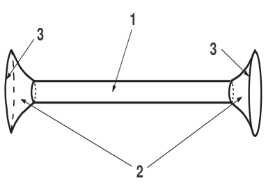
Figure 5: The approximate model of the $\Delta-$string. 1 is the long tube which is the part of the $Q=Q_{0}$ solution. 2 are two cones which are the $Q=0$ solutions, 3 are two hypersurfaces where $ds^{2}=0$.

For the model of the central tube we take the part of the infinite flux tube solution with $Q=Q_{0}$ [3]

$$a_{\infty}=\frac{Q_{0}^{2}}{2}=const,$$ (40)

$$e^{\psi}=\frac{a_{\infty}}{\Delta}=\cosh\frac{r}{\sqrt{a_{\infty}}},$$ (41)

$$\omega=\sqrt{2}\sinh\frac{r}{\sqrt{a_{\infty}}}$$ (42)

here we have parallel electric $E$ and magnetic $H$ fields with equal electric $q$ and magnetic $Q$ charges.

For a model of two peripheral ends (cones) we take the solution with $Q=0$ (equations (17)-(19)). Here we have only the electric field $E$ - (11). At the ends of the $\Delta-$string ($r=\pm r_{H}$) the function $\Delta(\pm r_{H})=0$ and the term $Q^{2}\Delta e^{2\psi}/a^{3}$ in equations (7)-(10) is zero that allows us to set this term as zero at the peripheral cones.

We have to join the components of metric on the $r=r_{1}=r_{H}-\sqrt{a(0)}$ (here $a(0)=a_{\infty}$).

$$\cosh^{2}\left(\frac{r_{1}}{\sqrt{a(0)}}\right)=\frac{\tilde{a}(r_{1})}{\tilde{\Delta}(r_{1})}=\tilde{g}_{tt}(r_{1})=\tilde{\tilde{g}}_{tt}(r_{1})=\frac{\tilde{\tilde{a}}(r_{1})}{\tilde{\tilde{\Delta}}(r_{1})}$$ (43)

here $\tilde{}$ and $\tilde{\tilde{}}$ mean that the corresponding quantities are the metric components for $Q=Q_{0}$ and $Q=0$ solutions respectively. According to equations (17)-(19)

$$\tilde{\tilde{a}}(r) = a(0)+\left(r-r_{1}\right)^{2},$$ (44)

$$\tilde{\tilde{\Delta}}(r) = \alpha\left[a(0)-\left(r-r_{1}\right)^{2}\right]$$ (45)

$$\tilde{\tilde{a}}(r_{1}) = \tilde{a}(r_{1})=a(0)$$ (46)

here $r_{0}^{2}$ from equation (17)-(19) is replaced with $\tilde{\tilde{a}}(0)$ and some coefficient $\alpha$ is introduced as equations (7)-(10) with $Q=0$ have the terms like $\Delta^{\prime\prime}/\Delta$ and $\Delta^{\prime}/\Delta$ only. It gives us

$$\alpha=\frac{1}{\cosh^{2}\left(\frac{r_{1}}{\sqrt{a(0)}}\right)}\approx 4e^{\frac{-2r_{1}}{\sqrt{a(0)}}}$$ (47)

since for the long $\Delta-$string $r_{1}/\sqrt{a(0)}\gg 1$. The next joining is for

$$1=\frac{\tilde{\Delta}(r_{1})e^{2\tilde{\psi}(r_{1})}}{\tilde{a}(r_{1})}=\tilde{g}_{55}(r_{1})=\tilde{\tilde{g}}_{55}(r_{1})=\frac{\tilde{\tilde{\Delta}}(r_{1})e^{2\tilde{\tilde{\psi}}(r_{1})}}{\tilde{\tilde{a}}(r_{1})}$$ (48)

here the constant term $2\tilde{\tilde{\psi}}_{1}$ is added to solution (19) $2\psi_{0}=0$ since again equations (7)-(10) have $\psi^{\prime\prime}$ and $\psi^{\prime}$ terms only. Consequently

$$e^{2\tilde{\tilde{\psi}}_{1}}=\frac{1}{\alpha}\approx\frac{e^{2r_{1}/\sqrt{a(0)}}}{4}\quad\text{or}\quad\psi_{1}\approx\frac{r_{1}}{\sqrt{a(0)}}-\ln 4.$$ (49)

The last component of the metric is

$$a(0)=a_{\infty}=\tilde{g}_{\theta\theta}(r_{1})=\tilde{\tilde{g}}_{\theta\theta}(r_{1})=\tilde{\tilde{a}}(r_{1}).$$ (50)

For the electric field we have

$$\tilde{E}(r_{1}) = \frac{qe^{\tilde{\psi}(r_{1})}}{a(0)}=\frac{q}{a(0)}\cosh\left(\frac{r_{1}}{\sqrt{a(0)}}\right)=\frac{q}{a(0)}\frac{1}{\sqrt{\alpha}}$$ (51)

$$\tilde{\tilde{E}}(r_{1}) = q\frac{\tilde{\tilde{a}}(r_{1})}{\tilde{\tilde{\Delta}}^{2}(r_{1})}e^{-3\tilde{\tilde{\psi}}(r_{1})}=\frac{q}{a(0)}\frac{1}{\sqrt{\alpha}}$$ (52)

and consequently

$$\tilde{E}(r_{1})=\tilde{\tilde{E}}(r_{1}).$$ (53)

Thus our final result for this section is that at the first rough approximation the $\Delta-$string looks like to a tube with constant cross section and two cones attached to its ends.

6 $\Delta-$string as a model of electric charge

In this section we want to present a model of attachment of the $\Delta-$string to a spacetime.

Maybe the most important question for the $\Delta-$string is : what will see an external observer living in the Universe to which the $\Delta-$string is attached. Whether he will see a dyon with electric and magnetic fields or an electric charge ? This question is not very simple as it is not very clear what is it the electric and magnetic fields on the $\Delta-$string. Are they the tensor $F_{\mu\nu}$ and fields $E_{i}$ and $H_{i}$

$$F_{\mu\nu} = \partial_{\mu}A_{\nu}-\partial_{\nu}A_{\mu},\quad\mu,\nu=0,1,2,3,$$ (54)

$$E_{i} = F_{0i},\quad i,j,k=1,2,3,$$ (55)

$$H_{i} = e_{ijk}F^{jk}$$ (56)

or something another that is like to an electric displacement $D_{i}=\varepsilon E_{i}$ and $H_{i}=\mu B_{i}$ ? The answer on this question depends on the way how we will continue the solution behind the hypersurface $r=\pm r_{H}$ (where $ds^{2}=0$). We have two possibilities : the first way is the simple continuation our solution to $|r|>r_{H}$, the second way is a string approach - attachment the $\Delta-$string to a spacetime. In the first case $\Delta(r)>0$ by $|r|<r_{H}$ and $\Delta(r)<0$ by $|r|>r_{H}$ it means that by $|r|>r_{H}$ the time and 5th coordinate $\chi$ becomes respectively space-like and time-like dimensions. It is not so good for us. The second approach is like to a string attached to a D-brane. We believe that physically the second way is more interesting.

Let us consider Maxwell equations in the 5D Kaluza-Klein theory

$$R_{5\mu}=\frac{1}{\sqrt{-g}}\partial_{\nu}\left(\sqrt{-g}g_{55}F^{\mu\nu}\right)=0$$ (57)

here $g=\det{g_{AB}=a^{4}\sin^{2}\theta e^{2\psi}}$. These 5D Maxwell equations are similar to Maxwell equations in the continuous media where the factor $\sqrt{-g}g_{55}$ is like to a permittivity for $R_{50}$ equation and a permeability for $R_{5i}$ equations. It allows us offer the following conditions for matching the electric and magnetic fields at the attachment point of $\Delta-$ string to the spacetime

$$\sqrt{-g_{\Delta}}{g_{\Delta}}_{55}F^{0i}_{\Delta} = \sqrt{-g}F^{0i}$$ (58)

$$\sqrt{-g_{\Delta}}{g_{\Delta}}_{55}F^{ij}_{\Delta} = \sqrt{-g}F^{ij}$$ (59)

here the subscript $\Delta$ means that this quantity is given on the $\Delta-$string and on l.h.s there are the quantities belonging to the $\Delta-$string and on the r.h.s. the corresponding quantities belong to the spacetime to which we want to attach the $\Delta-$string. As an example one can join the $\Delta-$string to the Reissner-Nordström solution with the metric

$$ds^{2}=e^{2\nu}dt^{2}-e^{-2\nu}dr^{2}-r^{2}\left(d\theta^{2}+\sin^{2}\theta d\varphi^{2}\right).$$ (60)

Then on the $\Delta-$string

$$\sqrt{-g_{\Delta}}{g_{\Delta}}_{55}F^{tr}_{\Delta}=-\frac{\Delta^{2}e^{3\psi}}{a}\omega^{\prime}=-a\frac{q}{a}$$ (61)

For the Reissner-Nordström solution

$$\sqrt{-g}F^{tr}=-r^{2}E_{r(RN)}.$$ (62)

Therefore after joining on the event horizon $r=r_{H}$ ($a=a_{H}$) we have

$$E_{r(RN)}=\frac{q}{a_{H}}$$ (63)

here we took into account that $a_{H}=r^{2}_{H}$.

For equation (59) we have

$$\sqrt{-g_{\Delta}}{g_{\Delta}}_{55}F^{\theta\varphi}_{\Delta}=\frac{Q\Delta e^{3\psi}}{a^{2}}.$$ (64)

On the surface of joining $\Delta(r_{H})=0$ consequently we have very unexpected result : the continuation of $F^{\theta\varphi}$ (and magnetic field $H_{r}$) from the $\Delta-$string to the spacetime (D-brane) gives us zero magnetic field $H_{r}$.

Finally our result for this section is that the $\Delta-$string can be attached to a spacetime by such a way that it looks like to an electric charge but not magnetic one. Such approach to the geometrical interpretation of electric charges suddenly explain why we do not observe magnetic charges in the world.

7 Discussion and conclusions

In this paper we have considered some interesting properties of the $\Delta-$string. We have shown that there is the relation (13) between the metric components. Physically this relation shows that the cross section of $\Delta-$string is the same order on the interval $(-r_{H},+r_{H})$. In fact we can choose the cross section as $\approx l_{Pl}$ that guarantees us that the cross section of $\Delta-$string is in Planck region everywhere between points $\pm r_{H}$ where the $\Delta-$string can be attached to D-branes.

It is shown that in some rough approximation the length of $\Delta-$string depends logarithmically from a small number which is connected with the difference between $1-Q/Q_{0}$.

The calculations presented here give us an additional certainty that the string can have an inner structure and in gravity such string is the $\Delta-$string. This approach is similar to Einstein point of view that the electron has an inner structure which can be described inside of a gravitational theory as a vacuum topologically non-trivial solution.

Another interesting peculiarity is that the gravitational flux tube solutions appear in a relatively simple matter in the classical 5D gravity. This is in contrast with quantum chromodynamic where receiving a flux tube stretched between quark and antiquark is an unresolved problem. In both cases strings are some approximation for the tubes. It is possible that it is a manifestation of some nontrivial mapping between a classical gravity and a quantum field theory.

It is necessary to note that similar idea was presented in Ref. [4] : the matching of two remote regions was done using 4D infinite flux tube which is the Levi-Civita - Bertotti - Robinson solution filled with the electric and magnetic fields.

8 Acknowledgment

I am very grateful to the ISTC grant KR-677 for the financial support.

References

- [1] V. Dzhunushaliev, Class. Quant. Grav., 19, 4817 (2002); V. Dzhunushaliev, Phys. Lett. B., 553, 289 (2003); V. Dzhunushaliev, “string - a hybrid between wormhole and string”, gr-qc/0301046.
- [2] T. Levi-Civita, Atti Acad. Naz. Lincei, 26, 519 (1917) ; B. Bertotti, Phys. Rev., 116, 1331 (1959); I. Robinson, Bull. Akad. Pol., 7, 351 (1959).
- [3] V. Dzhunushaliev and D. Singleton, Phys. Rev. D59, 064018 (1999).
- [4] E. I. Guendelman, Gen. Relat. Grav., 23, 1415 (1991).