Spin Foam Models for Quantum Gravity

Abstract

In this article we review the present status of the spin foam formulation of non-perturbative (background independent) quantum gravity. The article is divided in two parts. In the first part we present a general introduction to the main ideas emphasizing their motivations from various perspectives. Riemannian 3-dimensional gravity is used as a simple example to illustrate conceptual issues and the main goals of the approach. The main features of the various existing models for 4-dimensional gravity are also presented here. We conclude with a discussion of important questions to be addressed in four dimensions (gauge invariance, discretization independence, etc.).

In the second part we concentrate on the definition of the Barrett-Crane model. We present the main results obtained in this framework from a critical perspective. Finally we review the combinatorial formulation of spin foam models based on the dual group field theory technology. We present the Barrett-Crane model in this framework and review the finiteness results obtained for both its Riemannian as well as its Lorentzian variants.

1 Introduction

Quantum gravity, the theory expected to reconcile the principles of quantum mechanics and general relativity, remains a major challenge in theoretical physics (for a review of the history of quantum gravity see [1]). The main lesson of general relativity is that, unlike in any other interaction, space-time geometry is fully dynamical. This special feature of gravity precludes the possibility of representing fields on a fixed background geometry and severely constrains the applicability of standard techniques that are successful in the description of other interactions. Although the necessity of a background independent formulation of quantum gravity is widely recognized, there is a current debate about the means by which it should be implemented. In particular, it is not clear whether the non renormalizability of perturbative quantum gravity should be interpreted as an indication of the inconsistency of general relativity at high energies, the inconsistency of the background-dependent framework applied to gravity, or a combination of both.

According to the (background dependent) perspective of standard QFT [2], non renormalizability signals the inconsistency of the theory at high energies to be corrected by a more fundamental theory in the UV regime. A classical example of this is Fermi’s four-fermion theory as an effective description of the weak interaction. According to this view different approaches to quantum gravity have been defined in terms of modifications of general relativity based on supersymmetry, higher dimensions, strings, etc. The finiteness properties of the perturbative expansions (which are background dependent from the onset) are improved in these theories; however, the definition of a background independent quantization of such modifications remains open.

The approach of non perturbative quantum gravity is based on a different interpretation of the infinities in perturbative quantum gravity: it is precisely the perturbative (background dependent) techniques which are inconsistent with the fundamental nature of gravity. This view is strongly suggested by the predictions of the background independent canonical quantization of general relativity defined by loop quantum gravity. Loop quantum gravity (LQG) is a non perturbative formulation of quantum gravity based on the connection formulation of general relativity (for an reviews on the subject see [3, 4, 5, 6]). A great deal of progress has been made within the theory. At the mathematical level, the main achievement is the rigorous definition of the Hilbert space of quantum geometry, the regularization of geometric operators and the rigorous definition of the quantum Hamiltonian constraint (defining the quantum dynamics). States of quantum geometry are given by polymer-like excitations supported on graphs (spin network states). From the physical viewpoint its main prediction is the discreteness of geometry at the Planck scale. This provides a clear-cut understanding of the problem of UV divergences in perturbative general relativity: at the Planck scale the classical notion of space and time simply ceases to exist; therefore, it is the assumption of a fixed smooth background geometry (typically flat space-time) in perturbation theory that becomes inconsistent at high energies. The theory successfully incorporates interactions between quantum geometry and quantum matter in a way that is completely free of divergences [7]. The quantum nature of space appears as a physical regulator for the other interactions.

Dynamics is governed by the quantum Hamiltonian constraint. Even when this operator is rigorously defined [8] it is technically difficult to characterize its solution space. This is partly because the $3+1$-decomposition of space-time (necessary in the canonical formulation) breaks the manifest $4$-diffeomorphism invariance of the theory making awkward the analysis of dynamics. The situation is somewhat analogous to that in standard quantum field theory. In the Hamiltonian formulation of standard quantum field theory manifest Lorentz invariance is lost due to a particular choice of time slicing of Minkowski space-time. The formalism is certainly Lorentz invariant, but one has to work harder to show it explicitly. Manifest Lorentz invariance can be kept only in the Lagrangian (path-integral) quantization making the (formal) path integral a powerful device for analyzing relativistic dynamics.

Consequently, there has been growing interest in trying to define dynamics in loop quantum gravity from a $4$-dimensional covariant perspective. This has given rise to the so-called spin foam approach to quantum gravity. Its main idea is the construction of a rigorous definition of the path integral for gravity based on the deep insights obtained in the canonical framework of loop quantum gravity. In turn, the path integral provides a device to explicitly solve the dynamics: path-integral transition amplitudes can be shown to correspond to solutions of the quantum Hamiltonian constraint.

The underlying discreteness discovered in loop quantum gravity is crucial: in spin foam models the formal Misner-Hawking functional integral for gravity is replaced by a sum over combinatorial objects given by foam-like configurations (spin foams). A spin foam represents a possible history of the gravitational field and can be interpreted as a set of transitions through different quantum states of space. Boundary data in the path integral are given by the polymer-like excitations (spin network states) representing $3$-geometry states in loop quantum gravity. General covariance implies the absence of a meaningful notion of time and transition amplitudes are to be interpreted as defining the physical scalar product.

While the construction can be explicitly carried out in three dimensions there are additional technical difficulties in four dimensions. Various models have been proposed. A natural question is whether the infinite sums over geometries defining transition amplitudes would converge. In fact, there is no UV problem due to the fundamental discreteness and potential divergences are associated to the IR regime. There are recent results in the context of the Barrett-Crane model showing that amplitudes are well defined when the topology of the histories is restricted in a certain way.

The aim of this article is to provide a comprehensive review of the progress that has been achieved in the spin foam approach over the last few years and provide as well a self contained introduction for the interested reader that is not familiar with the subject. The article is divided into two fundamental parts. In the first part we present a general introduction to the subject including a brief summary of LQG in Section 2. We introduce the spin foam formulation from different perspectives in Section 3. In Section 4 we present a simple example of spin foam model: Riemannian $3$-dimensional gravity. We use this example as the basic tool to introduce the main ideas and to illustrate various conceptual issues. We review the different proposed models for $4$-dimensional quantum gravity in Section 5. Finally, in Section 6 we conclude the first part by analyzing the various conceptual issues that arise in the approach. The first part is a general introduction to the formalism; it is self contained and could be read independently.

One of the simplest and most studied spin foam model for $4$-dimensional gravity is the Barrett-Crane model [9, 10]. The main purpose of the second part is to present a critical survey of the different results that have been obtained in this framework and its combinatorial generalizations [11, 12, 13] based on the dual group field theory (GFT) formulation. In Section 7 we present a systematic derivation of the Barrett-Crane model from the $Spin(4)$ Plebanski’s formulation. This derivation follows an alternative path from that of [14, 15]; here we emphasize the connection to a simplicial action.

Spin foams can be thought of as Feynman diagrams. In fact a wide class of spin foam models can be derived from the perturbative (Feynman) expansion of certain dual group field theories (GFT) [16, 17]. A brief review of the main ideas involved is presented in Section 8. We conclude the second part by studying the GFT formulation of the Barrett-Crane model for both Riemannian and Lorentzian geometry. The definition of the actual models and the sketch of the corresponding finiteness proofs [18, 19, 20] are given in Section 9.

Part I Main ideas

2 Loop Quantum Gravity and Quantum Geometry

Loop quantum gravity is a rigorous realization of the quantization program established in the 60’s by Dirac, Wheeler, De-Witt, among others (for recent reviews see [3, 4, 6]). The technical difficulties of Wheeler’s ‘geometrodynamics’ are circumvent by the use of connection variables instead of metrics [21, 22, 23]. At the kinematical level, the formulation is similar to that of standard gauge theories. The fundamental difference is however the absence of any non-dynamical background field in the theory.

The configuration variable is an $SU(2)$-connection $A_{a}^{i}$ on a 3-manifold $\Sigma$ representing space. The canonical momenta are given by the densitized triad $E_{i}^{a}$. The latter encode the (fully dynamical) Riemannian geometry of $\Sigma$ and are the analog of the ‘electric fields’ of Yang-Mills theory.

In addition to diffeomorphisms there is the local $SU(2)$ gauge freedom that rotates the triad and transforms the connection in the usual way. According to Dirac, gauge freedoms result in constraints among the phase space variables which conversely are the generating functionals of infinitesimal gauge transformations. In terms of connection variables the constraints are

$${\cal G}_{i}={\cal D}_{a}E^{a}_{i}=0,\ \ \ \ {\cal C}_{a}=E_{k}^{b}F^{k}_{ba}=0,\ \ \ \ {\cal S}=\epsilon^{ijk}E^{a}_{i}E^{b}_{j}F_{ab\,k}+\cdots=0,$$ (1)

where ${\cal D}_{a}$ is the covariant derivative and $F_{ba}$ is the curvature of $A_{a}^{i}$. ${\cal G}_{i}$ is the familiar Gauss constraint—analogous to the Gauss law of electromagnetism—generating infinitesimal $SU(2)$ gauge transformations, ${\cal C}_{a}$ is the vector constraint generating space-diffeomorphism, and ${\cal S}$ is the scalar constraint generating ‘time’ reparameterization (there is an additional term that we have omitted for simplicity).

Loop quantum gravity is defined using Dirac quantization. One first represents (1) as operators in an auxiliary Hilbert space $\cal H$ and then solves the constraint equations

$$\hat{\cal G}_{i}\Psi=0,\ \ \ \ \hat{\cal C}_{a}\Psi=0,\ \ \ \ \hat{\cal S}\Psi=0.$$ (2)

The Hilbert space of solutions is the so-called physical Hilbert space ${\cal H}_{phys}$. In a generally covariant system quantum dynamics is fully governed by constraint equations. In the case of loop quantum gravity they represent quantum Einstein’s equations.

States in the auxiliary Hilbert space are represented by wave functionals of the connection $\Psi(A)$ which are square integrable with respect to a natural diffeomorphism invariant measure, the Ashtekar-Lewandowski measure [24] (we denote it ${\cal L}^{2}[{\cal A}]$ where ${\cal A}$ is the space of (generalized) connections). This space can be decomposed into a direct sum of orthogonal subspaces ${\cal H}=\bigoplus_{\gamma}{\cal H}_{\gamma}$ labeled by a graph $\gamma$ in $\Sigma$. The fundamental excitations are given by the holonomy $h_{\ell}(A)\in SU(2)$ along a path $\ell$ in $\Sigma$:

$$h_{\ell}(A)={\cal P}\ {\rm exp}\ \int_{\ell}A.$$ (3)

Elements of ${\cal H}_{\gamma}$ are given by functions

$$\Psi_{f,\gamma}(A)=f(h_{\ell_{1}}(A),h_{\ell_{2}}(A),\dots,h_{\ell_{n}}(A)),$$ (4)

where $h_{\ell}$ is the holonomy along the links $\ell\in\gamma$ and $f:SU(2)^{n}\rightarrow{\mathbb{C}}$ is (Haar measure) square integrable. They are called cylindrical functions and represent a dense set in $\cal H$ denoted $Cyl$.

Gauge transformations generated by the Gauss constraint act non-trivially at the endpoints of the holonomy, i.e., at nodes of graphs. The Gauss constraint (in (1)) is solved by looking at $SU(2)$ gauge invariant functionals of the connection (${\cal L}^{2}[{\cal A}]/{\cal G}$). The fundamental gauge invariant quantity is given by the holonomy around closed loops. An orthonormal basis of the kernel of the Gauss constraint is defined by the so called spin network states $\Psi_{\scriptscriptstyle\gamma,\{j_{\ell}\},\{\iota_{n}\}}(A)$ [25, 26, 27]. Spin-networks are defined by a graph $\gamma$ in $\Sigma$, a collection of spins $\{j_{\ell}\}$—unitary irreducible representations of $SU(2)$—associated with links $\ell\in\gamma$ and a collection of $SU(2)$ intertwiners $\{\iota_{n}\}$ associated to nodes $n\in\gamma$ (see Figure 1). The spin-network gauge invariant wave functional $\Psi_{\scriptscriptstyle\gamma,\{j_{\ell}\},\{\iota_{n}\}}(A)$ is constructed by first associating an $SU(2)$ matrix in the $j_{\ell}$-representation to the holonomies $h_{\ell}(A)$ corresponding to the link $\ell$, and then contracting the representation matrices at nodes with the corresponding intertwiners $\iota_{n}$, namely

$$\Psi_{\scriptscriptstyle\gamma,\{j_{\ell}\},\{\iota_{n}\}}(A)=\prod_{n\in\gamma}\ \iota_{n}\ \prod_{\ell\in\gamma}\ j_{\ell}[h_{\scriptscriptstyle\ell}(A)],$$ (5)

where $j_{\ell}[h_{\scriptscriptstyle\ell}(A)]$ denotes the corresponding $j_{\ell}$-representation matrix evaluated at corresponding link holonomy and the matrix index contraction is left implicit.

Figure 1: Spin-network state: At 3-valent nodes the intertwiner is uniquely specified by the corresponding spins. At 4 or higher valent nodes an intertwiner has to be specified. Choosing an intertwiner corresponds to decompose the $n$-valent node in terms of $3$-valent ones adding new virtual links (dashed lines) and their corresponding spins. This is illustrated explicitly in the figure for the two $4$-valent nodes.

The solution of the vector constraint is more subtle [24]. One uses group averaging techniques and the existence of the diffeomorphism invariant measure. The fact that zero lies in the continuous spectrum of the diffeomorphism constraint implies solutions to correspond to generalized states. These are not in $\cal H$ but are elements of the topological dual $Cyl^{*}$. However, the intuitive idea is quite simple: solutions to the vector constraint are given by equivalence classes of spin-network states up to diffeomorphism. Two spin-network states are considered equivalent if their underlying graphs can be deformed into each other by the action of a diffeomorphism.

This can be regarded as an indication that the smooth spin-network category could be replaced by something which is more combinatorial in nature so that diffeomorphism invariance becomes a derived property of the classical limit. LQG has been modified along these lines by replacing the smooth manifold structure of the standard theory by the weaker concept of piecewise linear manifold [32]. In this context, graphs defining spin-network states can be completely characterized using the combinatorics of cellular decompositions of space. Only a discrete analog of the diffeomorphism symmetry survives which can be dealt with in a fully combinatorial manner. We will take this point of view when we introduce the notion of spin foam in the following section.

Quantum geometry

The generalized states described above solve all of the constraints (1) but the scalar constraint. They are regarded as quantum states of the Riemannian geometry on $\Sigma$. They define the kinematical sector of the theory known as quantum geometry.

Geometric operators acting on spin network states can be defined in terms of the fundamental triad operators $\hat{E}^{a}_{i}$. The simplest of such operators is the area of a surface $S$ classically given by

$$A_{S}(E)=\int_{S}dx^{2}\sqrt{{\rm Tr}[n_{a}n_{b}E^{a}E^{b}]}$$ (6)

where $n$ is a co normal. The geometric operator $\hat{A}_{S}(E)$ can be rigorously defined by its action on spin network states [33, 34, 35]. The area operator gives a clear geometrical interpretation to spin-network states: the fundamental 1-dimensional excitations defining a spin-network state can be thought of as quantized ‘flux lines’ of area. More precisely, if the surface $S\subset\Sigma$ is punctured by a spin-network link carrying a spin $j$, this state is an eigenstate of $\hat{A}_{S}(E)$ with eigenvalue proportional to $\ell^{2}_{P}\sqrt{j(j+1)}$. In the generic sector—where no node lies on the surface—the spectrum takes the simple form

$$a_{S}(\{j\})=8\pi\iota\ell^{2}_{P}\sum_{i}\sqrt{j_{i}(j_{i}+1)},$$ (7)

where $i$ labels punctures and $\iota$ is the Imirzi parameter [36] . $a_{S}(\{j\})$ is the sum of single puncture contributions. The general form of the spectrum including the cases where nodes lie on $S$ has been computed in closed form [35].

The spectrum of the volume operator is also discrete [33, 34, 38, 39]. If we define the volume operator $\hat{V}_{\sigma}(E)$ of a $3$-dimensional region $\sigma\subset\Sigma$ then non vanishing eigenstates are given by spin-networks containing $n$-valent nodes in $\sigma$ for $n>3$. Volume is concentrated in nodes.

Quantum dynamics

In contrast to the Gauss and vector constraints, the scalar constraint does not have a simple geometrical meaning. This makes its quantization more involved. Regularization choices have to be made and the result is not unique. After Thiemann’s first rigorous quantization [40] other well defined possibilities have been found [41, 42, 43]. This ambiguity affects dynamics governed by

$$\hat{\cal S}\Psi=0.$$ (8)

The difficulty in dealing with the scalar constraint is not surprising. The vector constraint—generating space diffeomorphisms—and the scalar constraint—generating time reparameterizations—arise from the underlying $4$-diffeomorphism invariance of gravity. In the canonical formulation the $3+1$ splitting breaks the manifest $4$-dimensional symmetry. The price paid is the complexity of the time re-parameterization constraint $\cal S$. The situation is somewhat reminiscent of that in standard quantum field theory where manifest Lorentz invariance is lost in the Hamiltonian formulation .

From this perspective, there has been growing interest in approaching the problem of dynamics by defining a covariant formulation of quantum gravity. The idea is that (as in the QFT case) one can keep manifest $4$-dimensional covariance in the path integral formulation. The spin foam approach is an attempt to define the path integral quantization of gravity using what we have learn from LQG.

In standard quantum mechanics path integrals provide the solution of dynamics as a device to compute the time evolution operator. Similarly, in the generally covariant context it provides a tool to find solutions to the constraint equations (this has been emphasized formally in various places: in the case of gravity see for example [44], for a detailed discussion of this in the context of quantum mechanics see [45]). We will come back to this issue later.

Let us finish by stating some properties of $\hat{S}$ that do not depend on the ambiguities mentioned above. One is the discovery that smooth loop states naturally solve the scalar constraint operator [46, 47]. This set of states is clearly to small to represent the physical Hilbert space (e.g., they span a zero volume sector). However, this implies that $\hat{S}$ acts only on spin network nodes. Its action modifies spin networks at nodes by creating new links according to Figure 2 . This is crucial in the construction of the spin foam approach of the next section.

      $\begin{array}[]{c}\includegraphics[height=85.35826pt]{spin1.eps}\end{array}\ \ \rightarrow\ \ \begin{array}[]{c}\includegraphics[height=85.35826pt]{spin2.eps}\end{array}$

Figure 2: A typical transition generated by the action of the scalar constraint

3 Spin Foams and the path integral for gravity

The possibility of defining quantum gravity using Feynman’s path integral approach has been considered long ago by Misner and later extensively studied by Hawking, Hartle and others [48, 49]. Given a 4-manifold $\cal M$ with boundaries $\Sigma_{1}$ and $\Sigma_{2}$, and denoting by $G$ the space of metrics on ${\cal M}$, the transition amplitude between $\left|\left[q_{ab}\right]\right>$ on $\Sigma_{1}$ and $\left|\left[q^{\prime}_{ab}\right]\right>$ on $\Sigma_{2}$ is formally

$$\left<\left[q_{ab}\right]\right.\left|\right[q^{\prime}_{ab}\left]\right>=\int\limits_{\left[g\right]}{\cal D}[g]\ \ e^{iS([g])},$$ (9)

where the integration on the right is performed over all space-time metrics up to $4$-diffeomorphisms $\left[g\right]\in G/{\scriptstyle Diff({\cal M})}$ with fixed boundary values up to $3$-diffeomorphisms $\left[q_{ab}\right]$, $\left[q^{\prime}_{ab}\right]$, respectively.

There are various difficulties associated with (9). Technically there is the problem of defining the functional integration over $\left[g\right]$ on the RHS. This is partially because of the difficulties in defining infinite dimensional functional integration beyond the perturbative framework. In addition, there is the issue of having to deal with the space $G/{\scriptstyle Diff({\cal M})}$, i.e., how to characterize the diffeomorphism invariant information in the metric. This gauge problem ($3$-diffeomorphisms) is also present in the definition of the boundary data. There is no well defined notion of kinematical state $\left|\left[q_{ab}\right]\right>$ as the notion of kinematical Hilbert space in standard metric variables has never been defined.

We can be more optimistic in the framework of loop quantum gravity. The notion of quantum state of $3$-geometry is rigorously defined in terms of spin-network states. They carry the diff-invariant information of the Riemannian structure of $\Sigma$. In addition, and very importantly, these states are intrinsically discrete (colored graphs on $\Sigma$) suggesting a possible solution to the functional measure problem, i.e., the possibility of constructing a notion of Feynman ‘path integral’ in a combinatorial manner involving sums over spin network world sheets amplitudes. Heuristically, ‘$4$-geometries’ are to be represented by ‘histories’ of quantum states of $3$-geometries or spin network states. These ‘histories’ involve a series of transitions between spin network states (Figure  3), and define a foam-like structure (a ‘$2$-graph’ or $2$-complex) whose components inherit the spin representations from the underlying spin networks. These spin network world sheets are the so-called spin foams.

The precise definition of spin foams was introduced by Baez in [14] emphasizing their role as morphisms in the category defined by spin networks. A spin foam ${\cal F}:s\rightarrow s^{\prime}$, representing a transition from the spin-network $s=(\gamma,\{j_{\ell}\},\{\iota_{n}\})$ into $s^{\prime}=(\gamma^{\prime},\{j_{\ell^{\prime}}\},\{\iota_{n^{\prime}}\})$, is defined by a $2$-complex ${\cal J}$ bordered by the graphs of $\gamma$ and $\gamma^{\prime}$ respectively, a collection of spins $\{j_{f}\}$ associated with faces $f\in{\cal J}$ and a collection of intertwiners ${\{\iota_{e}}\}$ associated to edges $e\in{\cal J}$. Both spins and intertwiners of exterior faces and edges match the boundary values defined by the spin networks $s$ and $s^{\prime}$ respectively. Spin foams ${\cal F}:s\rightarrow s^{\prime}$ and ${\cal F}^{\prime}:s^{\prime}\rightarrow s^{\prime\prime}$ can be composed into ${\cal FF}^{\prime}:s\rightarrow s^{\prime\prime}$ by gluing together the two corresponding 2-complexes at $s^{\prime}$. A spin foam model is an assignment of amplitudes $A[{\cal F}]$ which is consistent with this composition rule in the sense that

$$A[{\cal FF}^{\prime}]=A[{\cal F}]A[{\cal F}^{\prime}].$$ (10)

Transition amplitudes between spin network states are defined by

$$\left<s,s^{\prime}\right>_{phys}=\sum_{{\cal F}:s\rightarrow s^{\prime}}A[{\cal F}],$$ (11)

where the notation anticipates the interpretation of such amplitudes as defining the physical scalar product. The domain of the previous sum is left unspecified at this stage. We shall discuss this question further in Section 6. This last equation is the spin foam counterpart of equation (9). This definition remains formal until we specify what the set of allowed spin foams in the sum are and define the corresponding amplitudes.

​​​​​​

      $\begin{array}[]{c}\includegraphics[height=128.0374pt]{spinfoam.eps}\end{array}\ \ \rightarrow\ \ \begin{array}[]{c}\includegraphics[height=128.0374pt]{spinfoam2.eps}\end{array}$

Figure 3: A typical path in a path integral version of loop quantum gravity is given by a series of transitions through different spin-network states representing a state of $3$-geometries. Nodes and links in the spin network evolve into 1-dimensional edges and faces. New links are created and spins are reassigned at vertexes (emphasized on the right). The ‘topological’ structure is provided by the underlying $2$-complex while the geometric degrees of freedom are encoded in the labeling of its elements with irreducible representations and intertwiners.

In standard quantum mechanics the path integral is used to compute the matrix elements of the evolution operator $U(t)$. It provides in this way the solution for dynamics since for any kinematical state $\Psi$ the state $U(t)\Psi$ is a solution to Schrödinger’s equation. Analogously, in a generally covariant theory the path integral provides a device for constructing solutions to the quantum constraints. Transition amplitudes represent the matrix elements of the so-called generalized ‘projection’ operator $P$ (Sections 3.1 and 6.3) such that $P\Psi$ is a physical state for any kinematical state $\Psi$. As in the case of the vector constraint the solutions of the scalar constraint correspond to distributional states (zero is in the continuum part of its spectrum). Therefore, ${\cal H}_{phys}$ is not a proper subspace of $\cal H$ and the operator $P$ is not a projector ($P^{2}$ is ill defined). In Section 4 we give an explicit example of this construction.

The background-independent character of spin foams is manifest. The $2$-complex can be thought of as representing ‘space-time’ while the boundary graphs as representing ‘space’. They do not carry any geometrical information in contrast with the standard concept of a lattice. Geometry is encoded in the spin labelings which represent the degrees of freedom of the gravitational field.

3.1 Spin foams and the projection operator into ${\cal H}_{\scriptscriptstyle phys}$

Spin foams naturally arise in the formal definition of the exponentiation of the scalar constraint as studied by Reisenberger and Rovelli in [53] and Rovelli [54]. The basic idea consists of constructing the ‘projection’ operator $P$ providing a definition of the formal expression

$$P=\prod_{x\in\Sigma}\delta(\hat{\cal S}(x))=\int{\cal D}[N]\ e^{i\hat{\cal S}[N]},$$ (12)

where $\hat{\cal S}[N]=\int dx^{3}N(x)\hat{\cal S}(x)$, with $N(x)$ the lapse function. $P$ defines the physical scalar product according to

$$\left<s,s^{\prime}\right>_{\scriptscriptstyle phys}=\left<sP,s^{\prime}\right>,$$ (13)

where the RHS is defined using the kinematical scalar product. Reisenberger and Rovelli make progress toward a definition of (12) by constructing a truncated version $P_{\Lambda}$ (where $\Lambda$ can be regarded as an infrared cutoff). One of the main ingredients is Rovelli’s definition of a diffeomorphism invariant measure ${\cal D}[N]$ generalizing the techniques of [55].

The starting point is the expansion of the exponential in (12) in powers

$$\left<sP_{\Lambda},s^{\prime}\right>=\int\limits_{|N(x)|\leq\Lambda}{\cal D}[N]\left<s\sum\limits^{\infty}_{n=0}\frac{i^{n}}{n!}({\cal S}[N])^{n},s^{\prime}\right>.$$ (14)

The construction works for a generic form of quantum scalar constraint as long as it acts locally on spin network nodes both creating and destroying links (this local action generates a vertex of the type emphasized in Figure 2). The action of $\hat{\cal S}[N]$ depends on the value of the lapse at nodes. Integration over the lapse can be performed and the final result is given by a power series in the cutoff $\Lambda$, namely

$$\left<sP_{\Lambda},s^{\prime}\right> = \sum\limits^{\infty}_{n=0}\ \frac{i^{n}\Lambda^{n}}{n!}\sum\limits_{{\cal F}_{n}:s\rightarrow s^{\prime}}A[{\cal F}_{n}]$$ (15)

$$= \sum\limits^{\infty}_{n=0}\ \frac{i^{n}\Lambda^{n}}{n!}\sum\limits_{{\cal F}_{n}:s\rightarrow s^{\prime}}\prod_{v}A_{v}(\rho_{v},\iota_{v}),$$

where ${\cal F}_{n}:s\rightarrow s^{\prime}$ are spin foams generated by $n$ actions of the scalar constraint, i.e., spin foams with $n$ vertices. The spin foam amplitude $A[{\cal F}_{n}]$ factorizes in a product of vertex contributions $A_{v}(\rho_{v},\iota_{v})$ depending of the spins $j_{v}$ and $\iota_{v}$ neighboring faces and edges. The spin foam shown in Figure 3 corresponds in this context to two actions of $\cal S$ and would contribute to the amplitude in the order $\Lambda^{2}$.

Physical observables can be constructed out of kinematical operators using $P$. If $O_{\scriptscriptstyle kin}$ represents an operator commuting with all but the scalar constraint then $O_{\scriptscriptstyle phys}=PO_{\scriptscriptstyle kin}P$ defines a physical observable. Its expectation value is

$$\left<O_{\scriptscriptstyle phys}\right>=\frac{\left<sPO_{\scriptscriptstyle kin}P,s\right>}{\left<sP,s\right>}:=\lim_{\Lambda\rightarrow\infty}\frac{\left<sP_{\Lambda}O_{\scriptscriptstyle kin}P_{\Lambda},s\right>}{\left<sP_{\Lambda},s\right>};$$ (16)

where the limit of the ratio of truncated quantities is expected to converge for suitable operators $O_{\scriptscriptstyle kin}$. Issues of convergence have not been studied and they would clearly be regularization dependent.

3.2 Spin foams from lattice gravity

Spin foam models naturally arise in lattice-discretizations of the path integral of gravity and generally covariant gauge theories. This was originally studied by Reisenberger [25]. The space-time manifold is replaced by a lattice given by a cellular complex. The discretization allows for the definition of the functional measure reducing the number of degrees of freedom to finitely many. The formulation is similar to that of standard lattice gauge theory. However, the nature of this truncation is fundamentally different: background independence implies that it cannot be simply interpreted as a UV regulator (we will be more explicit in the sequel).

We present a brief outline of the formulation for details see [25, 56, 57]. Start from the action of gravity in some first order formulation ($S(e,A)$). The formal path integral takes the form

$${Z}=\int{\cal D}[e]\ {\cal D}[A]\ e^{iS(e,A)}=\int{\cal D}[A]\ e^{iS_{\scriptscriptstyle\rm eff}(A)},$$ (17)

where in the second line we have formally integrated over the tetrad $e$ obtaining an effective action $S_{\scriptscriptstyle\rm eff}$. From this point on, the derivation is analogous to that of generally covariant gauge theory. The next step is to define the previous equation on a ‘lattice’.

As for Wilson’s action for standard lattice gauge theory the relevant structure for the discretization is a 2-complex ${\cal J}$. We assume the $2$-complex to be defined in terms of the dual $2$-skeleton ${\cal J}_{\Delta}$ of a simplicial complex $\Delta$. Denoting the edges $e\in{\cal J}_{\Delta}$ and the plaquettes or faces $f\in{\cal J}_{\Delta}$ one discretizes the connection by assigning a group element $g_{e}$ to edges

$$A\rightarrow\{g_{e}\}.$$

The Haar measure on the group is used to represent the connection integration:

$${\cal D}[A]\rightarrow\prod_{e\in{\cal J}_{\Delta}}dg_{e}.$$

The action of gravity depends on the connection $A$ only through the curvature $F(A)$ so that upon discretization the action is expressed as a function of the holonomy around faces $g_{f}$ corresponding to the product of the $g_{e}$’s which we denote $g_{f}=g^{\scriptscriptstyle(1)}_{e}\cdots g_{e}^{\scriptscriptstyle(n)}$:

$$F(A)\rightarrow\{g_{f}\}.$$

In this way, $S_{\scriptscriptstyle\rm eff}(A)\rightarrow S_{\scriptscriptstyle\rm eff}(\{g_{f}\})$. Thus the lattice path integral becomes:

$${Z}=\int\ \prod_{e\in{\cal J}_{\Delta}}\ dg_{e}\ {\rm exp}\left[{iS_{\rm eff}(\{g_{f}\})}\right].$$ (18)

Reisenberger assumes that $S_{\scriptscriptstyle\rm eff}(\{g_{f}\})$ is local in the following sense: the amplitude of any piece of the $2$-complex obtained as its intersection with a ball depends only on the value of the connection on the corresponding boundary. Degrees of freedom communicate through the lattice connection on the boundary. One can compute amplitudes of pieces of ${\cal J}_{\Delta}$ (at fixed boundary data) and then obtain the full ${\cal J}_{\Delta}$ amplitude by gluing the pieces together and integrating out the mutual boundary connections along common boundaries. The boundary of a portion of ${\cal J}_{\Delta}$ is a graph. The boundary value is an assignment of group elements to its links. The amplitude is a function of the boundary connection, i.e., an element of $Cyl$. In the case of a cellular 2-complex there is a maximal splitting corresponding to cutting out a neighborhood around each vertex. If the discretization is based on the dual of a triangulation these elementary building blocks are all alike and denoted atoms. Such an atom in four dimensions is represented in Figure 4.

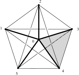
Figure 4: A fundamental atom is defined by the intersection of a dual vertex in ${\cal J}_{\Delta}$ (corresponding to a 4-simplex in $\Delta$) with a 3-sphere. The thick lines represent the internal edges while the thin lines the intersections of the internal faces with the boundary. They define the boundary graph denoted $\gamma_{5}$ below. One of the faces has been emphasized.

The atom amplitude depends on the boundary data given by the value of the holonomies on the ten links of the pentagonal boundary graph $\gamma_{5}$ shown in the figure. This amplitude can be represented by a function

$${\cal V}(\alpha_{ij})\ \ \ {\rm for}\ \ \ \alpha_{ij}\in G\ \ \ {\rm and}\ \ \ i\not=j=1,\dots,5$$ (19)

where $\alpha_{ij}$ represents the boundary lattice connection along the link $ij$ in Figure 4. Gauge invariance ($V(\alpha_{ij})=V(g_{i}\alpha_{ij}g^{-1}_{j})$) implies that the function can be spanned in terms of spin networks functions $\Psi_{\gamma_{5},\{\rho_{ij}\},\{\iota_{i}\}}(\alpha_{ij})$ based on the pentagonal graph $\gamma_{5}$, namely

$${\cal V}(\alpha_{ij})=\sum_{\rho_{ij}}\sum_{\iota_{i}}{\tilde{\cal V}}(\{\rho_{ij}\},\{\iota_{i}\})\ \Psi_{\gamma_{5},\{\rho_{ij}\},\{\iota_{i}\}}(\alpha_{ij})$$ (20)

where $\tilde{\cal V}(\{\rho_{ij}\},\{\iota_{i}\})$ is the atom amplitude in ‘momentum’ space depending on ten spins $\rho_{ij}$ labeling the faces and five intertwiners $\iota_{i}$ labeling the edges. Gluing the atoms together the integral over common boundaries is replaced by the sum over common values of spin labels and intertwiners. The total amplitude becomes

$$Z[{\cal J}_{\Delta}]=\sum_{{\cal C}_{f}:\{f\}\rightarrow\{\rho_{f}\}}\sum_{{\cal C}_{e}:\{e\}\rightarrow\{\iota_{e}\}}\prod_{f\in{{\cal J}_{\Delta}}}A_{f}(\rho_{f},\iota_{f})\ \prod_{v\in{{\cal J}_{\Delta}}}\tilde{\cal V}(\{\rho_{v}\},\{\iota_{v}\}),$$ (21)

where ${\cal C}_{e}:\{e\}\rightarrow\{\iota_{e}\}$ denotes the assignment of intertwiners to edges, ${\cal C}_{f}:\{\rho_{f}\}\rightarrow\{f\}$ the assignment of spins $\rho_{f}$ to faces, and $A_{f}(\rho_{f},\iota_{f})$ is the face amplitude arising in the integration over the lattice connection. The lattice definition of the path integral for gravity and covariant gauge theories becomes a discrete sum of spin foam amplitudes!

3.3 Spin foams for gravity from BF theory

The integration over the tetrad we formally performed in (17) is not always possible in practice. There is however a type of generally covariant theory for which the analog integration is trivial. This is the case of a class of theories called BF theory. General relativity in three dimensions is of this type. Consequently, BF theory can be quantized along the lines of the previous section. BF spin foam amplitudes are simply given by certain invariants in the representation theory of the gauge group. We shall study in some detail the case of $3$-dimensional Riemannian quantum gravity in the next section.

The relevance of BF theory is its close relation to general relativity in four dimensions. In fact, general relativity can be described by certain BF theory action plus Lagrange multiplier terms imposing certain algebraic constraints on the fields [58]. This is the starting point for the definition of several of the models we will present in this article: a spin foam model for gravity can be defined by imposing restrictions on the spin foams that enter in the partition function of the BF theory. These restrictions are essentially the translation into representation theory of the constraints that reduce BF theory to general relativity.

3.4 Spin foams as Feynman diagrams

As already pointed out in [14] spin foams can be interpreted in close analogy to Feynman diagrams. Standard Feynman graphs are generalized to $2$-complexes and the labeling of propagators by momenta to the assignment of spins to faces. Finally, momentum conservation at vertices in standard Feynmanology is now represented by spin-conservation at edges, ensured by the assignment of the corresponding intertwiners. In spin foam models the non-trivial content of amplitudes is contained in the vertex amplitude as pointed out in Sections 3.1 and 3.2 which in the language of Feynman diagrams can be interpreted as an interaction. We shall see that this analogy is indeed realized in the formulation of spin foam models in terms of a group field theory (GFT) [16, 17].

4 Spin foams for $3$-dimensional gravity

Three dimensional gravity is an example of BF theory for which the spin foam approach can be implemented in a rather simple way. Despite its simplicity the theory allows for the study of many of the conceptual issues to be addressed in four dimensions. In addition, as we mentioned in Section 3.3, spin foams for BF theory are the basic building block of $4$-dimensional gravity models. For a beautiful presentation of BF theory and its relation to spin foams see [59]. For simplicity we study the Riemannian theory; the Lorentzian generalization of the results of this section have been studied in [60].

4.1 The classical theory

Riemannian gravity in $3$ dimensions is a theory with no local degrees of freedom, i.e., no gravitons. Its action is given by

$$S(e,A)=\int\limits_{\cal M}Tr(e\wedge F(A)),$$ (22)

where the field $A$ is an $SU(2)$-connection and the triad $e$ is a Lie algebra valued $1$-form. The local symmetries of the action are $SU(2)$ gauge transformations

$$\delta e=\left[e,\omega\right],\ \ \ \ \ \ \ \ \ \delta A=d_{A}\omega,$$ (23)

where $\omega$ is a ${{\tt su(2)}}$-valued $0$-form, and ‘topological’ gauge transformation

$$\delta e=d_{\scriptscriptstyle A}\eta,\ \ \ \ \ \ \ \ \ \delta A=0,$$ (24)

where $d_{\scriptscriptstyle A}$ denotes the covariant exterior derivative and $\eta$ is a ${\tt su(2)}$-valued $0$-form. The first invariance is manifest from the form of the action, while the second is a consequence of the Bianchi identity, $d_{\scriptscriptstyle A}F=0$. The gauge freedom is so big that the theory has only global degrees of freedom. This can be checked directly by writing the equations of motion

$$F(A)=d_{\scriptscriptstyle A}A=0,\ \ \ \ \ \ \ \ \ d_{\scriptscriptstyle A}e=0.$$ (25)

The first implies that the connection is flat which in turn means that it is locally gauge ($A=d_{\scriptscriptstyle A}\omega$). The solutions of the second equation are also locally gauge as any closed form is locally exact ($e=d_{\scriptscriptstyle A}\eta$) . This very simple theory can be quantized in a direct manner.

4.2 Canonical quantization

Assuming ${\cal M}=\Sigma\times{\mathbb{R}}$ where $\Sigma$ is a Riemann surface representing space, the phase space of the theory is parameterized by the spatial connection $A$ (for simplicity we use the same notation as for the space-time connection) and its conjugate momentum $E$. The constraints that result from the gauge freedoms (23) and (24) are

$${\cal D}_{a}E^{a}_{i}=0,\ \ \ \ \ F(A)=0.$$ (26)

The first is the familiar Gauss constraint (in the notation of equation (1)), and we call the second the curvature constraint. There are $6$ independent constraints for the $6$ components of the connection, i.e., no local degrees of freedom. The kinematical setting is analogous to that of $4$-dimensional gravity and the quantum theory is defined along similar lines. The kinematical Hilbert space (quantum geometry) is spanned by $SU(2)$ spin-network states on $\Sigma$ which automatically solve the Gauss constraint. “Dynamics” is governed by the curvature constraint. The physical Hilbert space is obtained by restricting the connection to be flat and the physical scalar product is defined by a natural measure in the space of flat connections [59]. The distributional character of the solutions of the curvature constraint is manifest here. Different spin network states are physically equivalent when they differ by a null state (states with vanishing physical scalar product with all spin network states). This happens when the spin networks are related by certain skein relations. One can reconstruct ${\cal H}_{phys}$ directly from the skein relations which in turn can be found by studying the covariant spin foam formulation of the theory.

4.3 Spin foam quantization of 3d gravity

Here we apply the general framework of Section 3.2. This has been studied by Iwasaki in [61, 62]. The partition function, ${\cal Z}$, is formally given by

$${\cal Z}=\int{\cal D}[e]{\cal D}[A]\ \ e^{i\int_{\scriptscriptstyle\cal M}{\rm Tr}[e\wedge F(A)]},$$ (27)

where for the moment we assume ${\cal M}$ to be a compact and orientable. Integrating over the $e$ field in (27) we obtain

$${\cal Z}=\int{\cal D}[A]\ \ \delta\left(F(A)\right).$$ (28)

The partition function ${\cal Z}$ corresponds to the ‘volume’ of the space of flat connections on $\cal M$.

In order to give a meaning to the formal expressions above, we replace the $3$-dimensional manifold ${\cal M}$ with an arbitrary cellular decomposition $\Delta$. We also need the notion of the associated dual 2-complex of $\Delta$ denoted by ${\cal J}_{\Delta}$. The dual 2-complex ${\cal J}_{\scriptscriptstyle\Delta}$ is a combinatorial object defined by a set of vertices $v\in{\cal J}_{\scriptscriptstyle\Delta}$ (dual to 3-cells in $\Delta$) edges $e\in{\cal J}_{\scriptscriptstyle\Delta}$ (dual to 2-cells in $\Delta$) and faces $f\in{\cal J}_{\scriptscriptstyle\Delta}$ (dual to $1$-cells in $\Delta$).

The fields $e$ and $A$ have support on these discrete structures. The $su(2)$-valued $1$-form field $e$ is represented by the assignment of an $e\in{su(2)}$ to each $1$-cell in $\Delta$. The connection field $A$ is represented by the assignment of group elements $g_{e}\in SU(2)$ to each edge in ${\cal J}_{\scriptscriptstyle\Delta}$.

The partition function is defined by

$${\cal Z}(\Delta)=\int\prod_{f\in{\cal J}_{\scriptscriptstyle\Delta}}de_{f}\ \prod_{e\in{\cal J}_{\scriptscriptstyle\Delta}}dg_{e}\ e^{i{\rm Tr}\left[e_{f}U_{f}\right]},$$ (29)

where $de_{f}$ is the regular Lebesgue measure on ${\mathbb{R}}^{3}$, $dg_{e}$ is the Haar measure on $SU(2)$, and $U_{f}$ denotes the holonomy around faces, i.e., $U_{f}=g^{1}_{e}\dots g^{\scriptscriptstyle N}_{e}$ for $N$ being the number of edges bounding the corresponding face. Since $U_{f}\in SU(2)$ we can write it as $U_{f}=u^{0}_{f}\ {\mathbbm{1}}+F_{f}$ where $u^{0}_{f}\in{\mathbb{C}}$ and $F_{f}\in su(2)$. $F_{f}$ is interpreted as the discrete curvature around the face $f$. Clearly ${\rm Tr}[e_{f}U_{f}]={\rm Tr}[e_{f}F_{f}]$. An arbitrary orientation is assigned to faces when computing $U_{f}$. We use the fact that faces in ${\cal J}_{\scriptscriptstyle\Delta}$ are in one-to-one correspondence with $1$-cells in $\Delta$ and label $e_{f}$ with a face subindex.

Integrating over $e_{f}$, we obtain

$${\cal Z}(\Delta)=\int\ \prod_{e\in{\cal J}_{\scriptscriptstyle\Delta}}dg_{e}\ \prod_{f\in{\cal J}_{\scriptscriptstyle\Delta}}{\huge\delta}(g^{1}_{e}\dots g^{\scriptscriptstyle N}_{e}),$$ (30)

where $\delta$ corresponds to the delta distribution defined on ${\cal L}^{2}(SU(2))$. Notice that the previous equation corresponds to the discrete version of equation (28).

The integration over the discrete connection ($\prod_{e}dg_{e}$) can be performed expanding first the delta function in the previous equation using the Peter-Weyl decomposition [63]

$$\delta(g)=\sum\limits_{j\in{\rm irrep}(SU(2))}\Delta_{j}\ {\rm Tr}\left[j(g)\right],$$ (31)

where $\Delta_{j}=2j+1$ denotes the dimension of the unitary representation $j$, and $j(g)$ is the corresponding representation matrix. Using equation (31), the partition function (30) becomes

$${\cal Z}(\Delta)=\sum\limits_{{\cal C}:\{j\}\rightarrow\{f\}}\int\ \prod_{e\in{\cal J}_{\scriptscriptstyle\Delta}}dg_{e}\ \prod_{f\in{\cal J}_{\scriptscriptstyle\Delta}}\Delta_{j_{f}}\ {\rm Tr}\left[j_{f}(g^{1}_{e}\dots g^{\scriptscriptstyle N}_{e})\right],$$ (32)

where the sum is over coloring of faces in the notation of (21).

Going from equation (29) to (32) we have replaced the continuous integration over the $e$’s by the sum over representations of $SU(2)$. Roughly speaking, the degrees of freedom of $e$ are now encoded in the representation being summed over in (32).

Now it remains to integrate over the lattice connection $\{g_{e}\}$. If an edge $e\in{\cal J}_{\scriptscriptstyle\Delta}$ bounds $n$ faces there are $n$ traces of the form ${\rm Tr}[j_{f}(\cdots g_{e}\cdots)]$ in (32) containing $g_{e}$ in the argument. The relevant formula is

$$P^{n}_{inv}:=\int dg\ {j_{1}(g)}\otimes j_{2}(g)\otimes\cdots\otimes j_{n}(g)=\sum_{\iota}{C^{\scriptscriptstyle\iota}_{\scriptscriptstyle j_{1}j_{2}\cdots j_{n}}\ C^{*{\scriptscriptstyle\iota}}_{\scriptscriptstyle j_{1}j_{2}\cdots j_{n}}},$$ (33)

where $P^{n}_{inv}$ is the projector onto ${\rm Inv}[j_{1}\otimes j_{2}\otimes\cdots\otimes j_{n}]$. On the RHS we have chosen an orthonormal basis of invariant vectors (intertwiners) to express the projector. Notice that the assignment of intertwiners to edges is a consequence of the integration over the connection. This is not a particularity of this example but rather a general property of local spin foams as pointed out in Section 3.2. Finally (30) can be written as a sum over spin foam amplitudes

$${\cal Z}(\Delta)=\sum\limits_{{\cal C}:\{j\}\rightarrow\{f\}}\ \sum\limits_{{\cal C}:\{\iota\}\rightarrow\{e\}}\ \prod_{f\in{\cal J}_{\scriptscriptstyle\Delta}}\Delta_{j_{f}}\prod_{v\in{\cal J}_{\scriptscriptstyle\Delta}}A_{v}(\iota_{v},j_{v}),$$ (34)

where $A_{v}(\iota_{v},j_{v})$ is given by the appropriate trace of the intertwiners $\iota_{v}$ corresponding to the edges bounded by the vertex and $j_{v}$ are the corresponding representations. This amplitude is given in general by an $SU(2)$ $3Nj$-symbol corresponding to the flat evaluation of the spin network defined by the intersection of the corresponding vertex with a $2$-sphere. When $\Delta$ is a simplicial complex all the edges in ${\cal J}_{\Delta}$ are $3$-valent and vertices are $4$-valent (one such vertex is emphasized in Figure 3, the intersection with the surrounding $S^{2}$ is shown in dotted lines). Consequently, the vertex amplitude is given by the contraction of the corresponding four $3$-valent intertwiners, i.e., a $6j$-symbol. In that case the partition function takes the familiar Ponzano-Regge [64] form

$${\cal Z}(\Delta)=\sum\limits_{{\cal C}:\{j\}\rightarrow\{f\}}\ \prod_{f\in{\cal J}_{\scriptscriptstyle\Delta}}\Delta_{j_{f}}\prod_{v\in{\cal J}_{\scriptscriptstyle\Delta}}\begin{array}[]{c}\includegraphics[width=85.35826pt]{tetras.eps}\end{array},$$ (35)

were the sum over intertwiners disappears since ${\rm dim}({\rm Inv}[j_{1}\otimes j_{2}\otimes j_{3}])=1$ for $SU(2)$ and there is only one term in (33). Ponzano and Regge originally defined the amplitude (35) from the study of the asymptotic properties of the $6j$-symbol.

4.3.1 Discretization independence

A crucial property of the partition function (and transition amplitudes in general) is that it does not depend on the discretization $\Delta$. Given two different cellular decompositions $\Delta$ and $\Delta^{\prime}$ (not necessarily simplicial)

$$\tau^{-n_{0}}Z(\Delta)=\tau^{-n^{\prime}_{0}}Z(\Delta^{\prime}),$$ (36)

where $n_{0}$ is the number of 0-simplexes in $\Delta$ (hence the number of bubbles in ${\cal J}_{\Delta}$), and $\tau=\sum_{j}(2j+1)$ is clearly divergent which makes discretization independence a formal statement without a suitable regularization.

The sum over spins in (35) is typically divergent, as indicated by the previous equation. Divergences occur due to infinite volume factors corresponding to the topological gauge freedom (24)(see [65]). The factor $\tau$ in (36) represents such volume factor. It can also be interpreted as a $\delta(0)$ coming from the existence of a redundant delta function in (30). One can partially gauge fix this freedom at the level of the discretization. This has the effect of eliminating bubbles from the 2-complex.

In the case of simply connected $\Sigma$ the gauge fixing is complete. One can eliminate bubbles and compute finite transition amplitudes. The result is equivalent to the physical scalar product defined in the canonical picture in terms of the delta measure.

In the case of gravity with cosmological constant the state-sum generalizes to the Turaev-Viro model [66] defined in terms of $SU_{q}(2)$ with $q^{n}=1$ where the representations are finitely many. Heuristically, the presence of the cosmological constant introduces a physical infrared cutoff. Equation (36) has been proved in this case for the case of simplicial decompositions in [66], see also [67, 68]. The generalization for arbitrary cellular decomposition was obtained in [69].

4.3.2 Transition amplitudes

Transition amplitudes can be defined along similar lines using a manifold with boundaries. Given $\Delta$, ${\cal J}_{\Delta}$ then defines graphs on the boundaries. Consequently, spin foams induce spin networks on the boundaries. The amplitudes have to be modified concerning the boundaries to have the correct composition property (10). This is achieved by changing the face amplitude from $(\Delta_{j_{f}})$ to $(\Delta_{j_{\ell}})^{1/2}$ on external faces.

The crucial property of this spin foam model is that the amplitudes are independent of the chosen cellular decomposition [67, 69]. This allows for computing transition amplitudes between any spin network states $s=(\gamma,\{j\},\{\iota\})$ and $s^{\prime}=(\gamma,\{j^{\prime}\},\{\iota^{\prime}\})$ according to the following rules:

• Given ${\cal M}=\Sigma\times[0,1]$ (piecewise linear) and spin network states $s=(\gamma,\{j\},\{\iota\})$ and $s^{\prime}=(\gamma,\{j^{\prime}\},\{\iota^{\prime}\})$ on the boundaries—for $\gamma$ and $\gamma^{\prime}$ piecewise linear graphs in $\Sigma$—choose any cellular decomposition $\Delta$ such that the dual $2$-complex ${\cal J}_{\Delta}$ is bordered by the corresponding graphs $\gamma$ and $\gamma^{\prime}$ respectively (existence can be shown easily).

• Compute the transition amplitude between $s$ and $s^{\prime}$ by summing over all spin foam amplitudes (rescaled as in (36)) for the spin foams $F:s\rightarrow s^{\prime}$ defined on the $2$-complex ${\cal J}_{\Delta}$.

4.3.3 The generalized projector

We can compute the transition amplitudes between any element of the kinematical Hilbert space ${\cal H}$. Transition amplitudes define the physical scalar product by reproducing the skein relations of the canonical analysis. We can construct the physical Hilbert space by considering equivalence classes under states with zero transition amplitude with all the elements of ${\cal H}$, i.e., null states.

Figure 5: Elementary spin foams used to prove skein relations.

Here we explicitly construct a few examples of null states. For any contractible Wilson loop in the $j$ representation the state

$$\psi=(2j+1)\ s-\begin{array}[]{c}\includegraphics[width=28.45274pt]{ojey.eps}\end{array}\otimes s\ \ =_{\left.\right._{\left.\right._{\!\!\!\!\!\!\!\!\!\!\!\!\!phys}}}\ \ 0,$$ (40)

for any spin network state $s$, has vanishing transition amplitude with any element of ${\cal H}$. This can be easily checked by using the rules stated above and the portion of spin foam illustrated in Figure 5 to show that the two terms in the previous equation have the same transition amplitude (with opposite sign) for any spin-network state in ${\cal H}$. Using the second elementary spin foam in Figure 5 one can similarly show that

$$\begin{array}[]{ccc}\includegraphics[width=56.9055pt]{intu.eps}\end{array}-\begin{array}[]{c}\includegraphics[width=56.9055pt]{intu1.eps}\end{array}\ \ =_{\left.\right._{\left.\right._{\!\!\!\!\!\!\!\!\!\!\!\!\!phys}}}\ \ 0,$$ (43)

or the re-coupling identity using the elementary spin foam on the right of Figure 5

$$\begin{array}[]{ccc}\includegraphics[width=56.9055pt]{intu1.eps}\end{array}-\sum\limits_{e}\sqrt{2s+1}\sqrt{2e+1}\left\{\begin{array}[]{ccc}i\ \ j\ \ s\\ k\ \ l\ \ e\end{array}\right\}\begin{array}[]{c}\includegraphics[height=56.9055pt]{intu2.eps}\end{array}\ \ =_{\left.\right._{\left.\right._{\!\!\!\!\!\!\!\!\!\!\!\!\!phys}}}\ \ 0,$$ (48)

where the quantity in brackets represents an $SU(2)$ $6j$-symbol. All skein relations can be found in this way. The transition amplitudes imply the skein relations that define the physical Hilbert space! The spin foam quantization is equivalent to the canonical one.

4.3.4 The continuum limit

Recently Zapata [70] formalized the idea of a continuum spin foam description of $3$-dimensional gravity using projective techniques inspired by those utilized in the canonical picture [24]. The heuristic idea is that due to the discretization invariance one can define the model in an ‘infinitely’ refined cellular decomposition that contains any possible spin network state on the boundary (this intuition is implicit in our rules for computing transition amplitudes above). Zapata concentrates on the case with non-vanishing cosmological constant and constructs the continuum extension of the Turaev-Viro model.

4.4 Conclusion

We have illustrated the general notion of the spin foam quantization in the simple case of $3$ dimensional Riemannian gravity (for the generalization to the Lorentzian case see [60]). The main goal of the approach is to provide a definition of the physical Hilbert space. The example of this section sets the guiding principles of what one would like to realize in four dimensions. However, as should be expected, there are various new issues that make the task by far more involved.

5 Spin foams for $4$-dimensional quantum gravity

In this section we briefly describe the various spin foam models for quantum gravity in the literature.

5.1 The Reisenberger model

According to Plebanski [58] the action of self dual Riemannian gravity can be written as a constrained $SU(2)$ BF theory

$$S(B,A)=\int{\rm Tr}\left[B\wedge F(A)\right]-\psi_{ij}\left[B^{i}\wedge B^{j}-\frac{1}{3}\delta^{ij}B^{k}\wedge B_{k}\right],$$ (49)

where variations with respect to the symmetric (Lagrange multiplier) tensor $\psi_{ij}$ imposes the constraints

$$\Omega^{ij}=B^{i}\wedge B^{j}-\frac{1}{3}\delta^{ij}B^{k}\wedge B_{k}=0.$$ (50)

When $B$ is non degenerate the constraints are satisfied if and only if $B^{i}=\pm(e^{0}\wedge e^{i}+{\scriptstyle\frac{1}{2}}\epsilon^{i}_{\ jk}e^{j}\wedge e^{k})$ which reduces the previous action to that of self-dual general relativity. Reisenberger studied the simplicial discretization of this action in [56] as a preliminary step toward the definition of the corresponding spin foam model. The consistency of the simplicial action is argued by showing that the simplicial theory converges to the continuum formulation when the triangulation is refined: both the action and its variations (equations of motion) converge to those of the continuum theory.

In reference [57] Reisenberger constructs a spin foam model for this simplicial theory by imposing the constraints $\Omega^{ij}$ directly on the $SU(2)$ BF amplitudes. The spin foam path integral for BF theory is obtained as in Section 4. The constraints are imposed by promoting the $B^{i}$ to operators ${\chi}^{i}$ (combinations of left/right invariant vector fields) acting on the discrete connection . The model is defined as

$$Z_{GR}={\underbrace{\int\ \ \prod_{e\in{\cal J}_{\scriptscriptstyle\Delta}}dg_{e}}_{\int{\cal D}[A]}}\ \overbrace{\delta(\hat{\Omega}^{ij})}^{\int{\cal D}[\psi]\ e^{i\psi_{ij}\Omega^{ij}}}\!\!\underbrace{\sum\limits_{{\cal C}:\{j\}\rightarrow\{f\}}\prod_{f\in{\cal J}_{\scriptscriptstyle\Delta}}\Delta_{j_{f}}\ {\rm Tr}\left[j_{f}(g^{1}_{e}\dots g^{\scriptscriptstyle N}_{e})\right]}_{\int{\cal D}[B]\ e^{i\int{\rm Tr}[B\wedge F(A)]}},$$ (52)

where $\hat{\Omega}={\cal J}^{i}\wedge{\cal J}^{j}-\frac{1}{3}\delta^{ij}{\cal J}^{k}\wedge{\cal J}_{k}$ and we have indicated the correspondence of the different terms with the continuum formulation. The preceding equation is rather formal; for the rigorous implementation see [57]. Reisenberger uses locality so that constraints are implemented on a single $4$-simplex amplitude. There is however a difficulty with the this procedure: the algebra of operators $\hat{\Omega}^{ij}$ do not close so that imposing the constraints sharply becomes a too strong condition on the BF configurations. In order to avoid this, Reisenberger defines a one-parameter family of models by inserting the operator

$$e^{-\frac{1}{2z^{2}}\hat{\Omega}^{2}}$$ (53)

instead of the delta function above. In the limit $z\rightarrow\infty$ the constraints are sharply imposed. This introduces an extra parameter to the model. The properties of the kernel of $\hat{\Omega}$ have not been studied in detail.

5.2 The Freidel-Krasnov prescription

In reference [71] Freidel and Krasnov define a general framework to construct spin foam models corresponding to theories whose action has the general form

$$S(B,A)=\int{\rm Tr}\left[B\wedge F(A)\right]+\Phi(B),$$ (54)

where the first term is the BF action while $\Phi(B)$ is a certain polynomial function of the $B$ field. The formulation is constructed for compact internal groups. The definition is based on the formal equation

$$\int{\cal D}[{B}]{\cal D}[{A}]\ e^{i\int{\rm Tr}\left[B\wedge F(A)\right]+\Phi(B)}:=\left.e^{i\int\Phi(\frac{\delta}{\delta J})}Z[J]\right|_{J=0},$$ (55)

where the generating functional $Z[J]$ is defined as

$$Z[J]:=\int{\cal D}[{B}]{\cal D}[{A}]\ e^{i\int{\rm Tr}\left[B\wedge F(A)\right]+{\rm Tr}\left[B\wedge J\right]},$$ (56)

where $J$ is an algebra valued $2$-form field. They provide a rigorous definition of the generating functional by introducing a discretization of $\cal M$ in the same spirit of the other spin foam models discussed here. Their formulation can be used to describe various theories of interest such as BF theories with cosmological terms, Yang-Mills theories (in $2$ dimensions) and Riemannian self-dual gravity. In the case of self dual gravity $B$ and $A$ are valued in $su(2)$, while

$$\Phi(B)=\int\psi_{ij}\left[B^{i}\wedge B^{j}-\frac{1}{3}\delta^{ij}B^{k}\wedge B_{k}\right]$$ (57)

according to equation (49). The model obtained in this way is very similar to Reisenberger’s one. There are however some technical differences. One of the more obvious one is that the non-commutative invariant vector fields ${\cal J}^{i}$ representing $B^{i}$ are replaced here by the commutative functional derivatives $\delta/\delta J^{i}$. The explicit properties of these models have not been studied further.

5.3 The Iwasaki model

Iwasaki defines a spin foam model of self dual Riemannian gravity by a direct lattice discretization of the continuous Ashtekar formulation of general relativity. This model constitutes an example of the general prescription of Section 3.2. The action is

$$S(e,A)=\int dx^{4}\ \epsilon^{\mu\nu\lambda\sigma}\left[2\ e^{0}_{[\mu}e_{\nu]i}+\epsilon^{0}_{\ ijk}e^{j}_{\mu}e^{k}_{\nu}\right]\left[2\ \partial_{[\lambda}A_{\sigma]}^{i}+\epsilon^{0i}_{\ \ lm}A^{l}_{\lambda}A^{m}_{\sigma}\right],$$ (58)

where $A^{i}_{a}$ is an $SU(2)$ connection. The fundamental observation of [73] is that one can write the discrete action in a very compact form if we encode part of the degrees of freedom of the tetrad in an $SU(2)$ group element. More precisely, if we take $g_{\mu\mu}=e^{i}_{\mu}e^{j}_{\mu}\delta_{ij}=1$ we can define ${\mathbf{e}}_{\mu}:=e_{\mu}^{0}+i\sigma_{i}e^{i}_{\mu}\in SU(2)$ where $\sigma_{i}$ are the Pauli matrices. In this parameterization of the ‘angular’ components of the tetrad and using a hypercubic lattice the discrete action becomes

$$S_{\Delta}=-\beta\sum_{v\in\Delta}\epsilon^{\mu\nu\lambda\sigma}{r_{\mu}r_{\nu}}\ {\rm Tr}\left[{\mathbf{e}}^{\dagger}_{\mu}{\mathbf{e}}_{\nu}U_{\lambda\sigma}\right],$$ (59)

where $r_{\mu}:=(\beta^{1/2}\ell_{p})^{-1}\epsilon\sqrt{g_{\mu\mu}}$, $U_{\mu\nu}$ is the holonomy around the $\mu\nu$-plaquette, $\epsilon$ the lattice constant and $\beta$ is a cutoff for $r_{\mu}$ used as a regulator ($r_{\mu}\leq\beta^{1/2}\ell_{p}\epsilon^{-1}$). The lattice path integral is defined by using the Haar measure both for the connection and the ‘spherical’ part of the tetrad $\mathbf{e}$’s and the radial part $dr_{\mu}:=dr_{\mu}r^{3}_{\mu}$. The key formula to obtain an expression involving spin foams is

$$e^{i{x}{\rm Tr}[U]}=\sum_{j}(2j+1)\frac{J_{2j+1}(2x)}{x}\chi_{j}(U).$$ (60)

Iwasaki writes down an expression for the spin foam amplitudes in which the integration over the connection and the $\mathbf{e}$’s can be computed explicitly. Unfortunately, the integration over the radial variables $r$ involves products of Bessel functions and its behavior is not analyzed in detail. In $3$ dimensions the radial integration can be done and the corresponding amplitudes coincide with the results of Section (4.3).

5.4 The Barrett-Crane model

The appealing feature of the previous models is the clear connection to loop quantum gravity, since they are defined directly using the self dual formulation of gravity (boundary states are $SU(2)$-spin networks). The drawback is the lack of closed simple expressions for the amplitudes which complicates their analysis. There is however a simple model that can be obtained as a systematic quantization of simplicial $SO(4)$ Plebanski’s action. This model was introduced by Barrett and Crane in [9] and further motivated by Baez in [14]. The basic idea behind the definition was that of the quantum tetrahedron introduced by Barbieri in [74] and generalized to 4d in [15]. The beauty of the model resides in its remarkable simplicity. This has stimulated a great deal of explorations and produced many interesting results. We will review most of these in Section 7.

5.5 Markopoulou-Smolin causal spin networks

Using the kinematical setting of LQG with the assumption of the existence of a micro-local (in the sense of Planck scale) causal structure Markopoulou and Smolin define a general class of (causal) spin foam models for gravity [75, 76] (see also [77]). The elementary transition amplitude $A_{s_{I}\rightarrow s_{I+1}}$ from an initial spin network $s_{I}$ to another spin network $s_{I+1}$ is defined by a set of simple combinatorial rules based on a definition of causal propagation of the information at nodes. The rules and amplitudes have to satisfy certain causal restrictions (motivated by the standard concepts in classical Lorentzian physics). These rules generate surface-like excitations of the same kind we encounter in the more standard spin foam model but endow the foam with a notion of causality. Spin foams ${\cal F}^{N}_{s_{i}\rightarrow s_{f}}$ are labeled by the number of times these elementary transitions take place. Transition amplitudes are defined as

$$\left<s_{i},s_{f}\right>=\sum_{N}\prod\limits^{N-1}_{I=0}A_{s_{I}\rightarrow s_{I+1}}.$$ (61)

The models are not related to any continuum action. The only guiding principles are the restrictions imposed by causality, simplicity and the requirement of the existence of a non-trivial critical behavior that would reproduce general relativity at large scales. Some indirect evidence of a possible non trivial continuum limit has been obtained in some versions of the model in $1+1$ dimensions.

5.6 Gambini-Pullin model

In reference [78] Gambini and Pullin introduced a very simple model obtained by modification of the $BF$ theory skein relations. As we argued in Section 4 skein relations defining the physical Hilbert space of BF theory are implied by the spin foam transition amplitudes. These relations reduce the large kinematical Hilbert space of $BF$ theory (analogous to that of quantum gravity) to a physical Hilbert space corresponding to the quantization of a finite number of degrees of freedom. Gambini and Pullin define a model by modifying these amplitudes so that some of the skein relations are now forbidden. This simple modification frees local excitations of a field theory. A remarkable feature is that the corresponding physical states are (in a certain sense) solutions to various regularizations of the scalar constraint for (Riemannian) LQG. The fact that physical states of BF theory solve the scalar constraint is well known [79], since roughly $F(A)=0$ implies $EEF(A)=0$. The situation here is of a similar nature, and—as the authors argue—one should interpret this result as an indication that some ‘degenerate’ sector of quantum gravity might be represented by this model. The definition of this spin foam model is not explicit since the theory is directly defined by the physical skein relations.

5.7 Capovilla-Dell-Jacobson theory on the lattice

The main technical difficulty that we gain in going from $3$-dimensional general relativity to the $4$-dimensional one is that the integration over the $e$’s becomes intricate. In the Capovilla-Dell-Jacobson [80, 81] formulation of general relativity this ‘integration’ is partially performed at the continuum level. The action is

$$S(\eta,A)=\int\eta{\rm Tr}\left[\epsilon\cdot F(A)\wedge F(A)\epsilon\cdot F(A)\wedge F(A)\right],$$ (62)

where $\epsilon\cdot F\wedge F:=\epsilon^{abcd}F_{ab}F_{cd}$. Integration over $\eta$ can be formally performed in the path integral and we obtain

$$Z=\int\prod_{x}\delta\left({\rm Tr}\left[\epsilon\cdot F(A)\wedge F(A)\epsilon\cdot F(A)\wedge F(A)\right]\right),$$ (63)

This last expression is of the form (17) and can be easily discretized along the lines of Section 3.2. The final expression (after integrating over the lattice connection) involves a sum over spin configurations with no implicit integrations. One serious problem of this formulation is that it corresponds to a sector of gravity where the Weyl tensor satisfy certain algebraic requirements. In particular flat geometries are not contained in this sector.

6 Some conceptual issues

6.1 Anomalies and gauge fixing

As we mentioned before and illustrated with the example of Section 4, the spin foam path integral is meant to provide a definition of the physical Hilbert space. Spin foam transition amplitudes are not interpreted as defining propagation in time but rather as defining the physical scalar product. This interpretation of spin foam models is the only one consistent with general covariance. However, in the path integral formulation, this property relies on the gauge invariance of the path integral measure. If the measure meets this property we say it is anomaly free. It is well known that in addition to the invariance of the measure, one must provide appropriate gauge fixing conditions for the amplitudes to be well defined. In this section we analyze these issues in the context of the spin foam approach.

Since we are interested in gravity in the first order formalism, in addition to diffeomorphism invariance one has to deal with the gauge transformations in the internal space. Let us first describe the situation for the latter. If this gauge group is compact then anomaly free measures are defined using appropriate variables and invariant measures. In this case gauge fixing is not necessary for the amplitudes to be well defined. Examples where this happens are: the models of Riemannian gravity considered in this paper (the internal gauge group being $SO(4)$ or $SU(2)$), and standard lattice gauge theory. In these cases, one represents the connection in terms of group elements (holonomies) and uses the (normalized) Haar measure in the integration. In the Lorentzian sector (internal gauge group $SL(2,{\mathbb{C}})$) the internal gauge orbits have infinite volume and the lattice path integral would diverge without an appropriate gauge fixing condition. These conditions generally exist in spin foam models and we will study an example in Section 9 (for a general treatment see [82]).

The remaining gauge freedom is diffeomorphism invariance. It is generally assumed that spin foam encode diff-invariant information about $4$-geometries. Thus, no gauge fixing would be necessary as one would be already summing over physical configurations. To illustrate this perspective we concentrate on the case of a model defined on a fixed discretization $\Delta$ as described in Section 3.2.

Let us start by considering the spin network states, at $\partial\Delta$: boundary of $\Delta$, for which we want to define the transition amplitudes. According to what we have learned from the canonical approach, $3$-diffeomorphism invariance is implemented by considering (diffeomorphism) equivalence classes of spin-network states. In the context of spin foams, the underlying discretization $\Delta$ restricts the graphs on the boundary to be contained on the dual $1$-skeleton of the boundary complex $\partial\Delta$. These states are regarded as representative elements of the corresponding $3$-diffeomorphism equivalence class. The discretization can be interpreted, in this way, as a gauge fixing of $3$-diffeomorphisms on the boundary. This gauge fixing is partial in the sense that, generically, there will remain a discrete symmetry remnant given by the discrete symmetries of the spin network. This remaining symmetry has to be factored out when computing transition amplitudes (in fact this also plays a role in the definition of the kinematical Hilbert space of Section 2).

The standard view point (consistent with LQG and quantum geometry) is that this should naturally generalize to $4$-diffeomorphisms for spin foams. The underlying $2$-complex ${\cal J}_{\Delta}$ on which spin foams are defined represents a partial gauge fixing for the configurations (spin foams) entering in the path integral. The remaining symmetry, to be factored out in the computation of transition amplitudes, corresponds simply to the finite group of discrete symmetries of the corresponding spin foams. This factorization is well defined since the number of equivalent spin foams can be characterized in a fully combinatorial manner, and is finite for any spin foam defined on a finite discretization. In addition, a spin foam model is anomaly free if the amplitudes are invariant under this discrete symmetry. This requirement is met by all the spin foam models we considered in this article.

We illustrate the intuitive idea of the previous paragraph in Figure 6. On the diagram $(a)$ a continuum configuration is represented by a discrete (spin foam) configuration on the lattice. On $(b)$ two configurations are shown. In the background dependent context (e.g., lattice gauge theory) these two configurations would be physically inequivalent as the lattice carries metric information (length of the edges). In the context of spin foam models there is no geometric information encoded in the discretization and in an anomaly free spin foam model the two configurations should be regarded as equivalent.

      $\begin{array}[]{c}\includegraphics[height=71.13188pt]{grid.eps}\end{array}\ \ \begin{array}[]{ccc}\rightarrow\\ (a)\end{array}\ \ \begin{array}[]{c}\includegraphics[height=71.13188pt]{grid3.eps}\end{array}\ \ \ \ \ \ \ \begin{array}[]{c}\includegraphics[height=71.13188pt]{grid5.eps}\end{array}\ \ \begin{array}[]{ccc}\rightarrow\\ (b)\end{array}\ \ \begin{array}[]{c}\includegraphics[height=71.13188pt]{grid6.eps}\end{array}$

Figure 6: Diffeomorphisms are replaced by discrete symmetries in spin foams. In this simplified picture there are two possible colorings of $0$ or $1$, the latter represented by the darkening of the corresponding lattice element. The two configurations on $(b)$ are regarded as physically equivalent in the background independent context.

The discretization of the manifold $\Delta$ is seen as a regulator introduced to define the spin foam model. Even when the regulator (or the discretization dependence) eventually has to be removed (see next subsection), the theory remains discrete at the fundamental level. The smooth manifold diffeomorphism invariant description is regarded in this context as a derived concept in the (low energy) continuum limit. Fundamental excitations are intrinsically discrete. From this viewpoint, the precise meaning of the gauge symmetries of such a theory would have to be formulated directly at the discrete level. We have seen that this can be achieved in the case of $3$-dimensional gravity (recall Section 4.3.1). From this perspective, the discrete symmetries of colored $2$-complexes (spin foams) represent the fundamental ‘gauge’ freedom. This symmetry would manifest itself as diffeomorphisms only in the continuum limit.

The viewpoint stated above is consistent with recent results obtained by Gambini and Pullin [83, 84]. They study the canonical formulation of theories defined on a lattice from the onset. This provides a way to analyze the meaning of gauge symmetries directly à la Dirac. Their results indicate that diff-invariance is indeed broken by the discretization in the sense that there is no infinitesimal generator of diffeomorphism. This is consistent with our covariant picture of discrete symmetries above. In their formulation the canonical equations of motion fix the value of what were Lagrange multipliers in the continuum (e.g. lapse and shift). This is interpreted as a breaking of diffeomorphism invariance; however, the solutions of the multiplier equations are highly non unique. The ambiguity in selecting a particular solution corresponds to the remnant diffeomorphism invariance of the discrete theory.

However, the notion of anomaly freeness stated at the beginning of this section should be strengthened. In fact according to our tentative definition, an anomaly free measure can be multiplied by any gauge invariant function and yield a new anomaly free measure. This kind of ambiguity is not what we want; however, it is in fact present in most of the spin foam models defined so far. In standard QFT theory, the formal (phase space) path integral measure in the continuum has a unique meaning (up to a constant normalization) emerging from the canonical formulation. Provided an appropriate gauge fixing, the corresponding Dirac bracket determines the formal measure on the gauge fixed constraint surface. As we will see later, there is a certain degree of ambiguity in the definition of various spin foam models in four dimensions. This ambiguity concerns the evaluation of lower dimensional simplexes and is directly related to the definition of measure in the spin foam sum. One would expect that a strengthened definition of anomaly freeness should resolve these ambiguities. This possibility is studied in [85].

Finally let us briefly recall the situation in $3$-dimensional gravity. In three dimensions the discrete action is invariant under transformations that are in correspondence with the continuum gauge freedoms (23) and (24). As we mentioned in Section 4.3.1 spin foam amplitudes diverge due to (24). This means that spin foams do not fix (24) up to a ‘finite volume’ discrete symmetry, which seems to be in conflict with the argument stated above as diffeomorphism can be obtained combining the transformations (23) and (24). However, the topological gauge symmetry (24) involves more than just diffeomorphisms. Indeed, only on shell one can express diffeomorphisms as a combination of (23) and (24). This representation of diffeomorphisms turns out to be field dependent (recall Footnote 11). At the canonical level we have seen that the topological symmetry (24) acts in away that is totally different from diffeomorphisms. In particular spin network states defined on graphs which which differ in the number of edges and vertices can be physically equivalent (recall Section 4.3.3). Thus $3$-dimensional gravity is a degenerate example and extrapolation of its gauge properties to four dimensions seems misleading.

In Section 7.1 we will study the spin foam quantization of BF theory—a topological theory which corresponds to a generalization of $3$-dimensional gravity to four dimensions. The spin foam amplitudes are also divergent in this case due to the analog of the gauge symmetry (24). Some of the spin foam models in Section 5 are defined from BF theory by implementing constraints that reduce the topological theory to general relativity. The implementation of the constraints breaks the topological symmetry (24) and the resulting model is no longer topological invariant. At the continuum level it is clear that the remnant gauge symmetry is diffeomorphism invariance. Whether in the the resulting spin foam model for gravity remnant is larger than the discrete spin foam symmetries advocated above has not been studied in detail.

The action of diffeomorphism is far from understood at a rigorous level in the context of spin foam models. Here we have presented an account of some of the ideas under consideration, and we tried to point out the relevance of an issue that certainly deserves detailed investigation.

6.2 Discretization dependence

The spin foam models we have introduced so far are defined on a fixed cellular decomposition of $\cal M$. This is to be interpreted as an intermediate step toward the definition of the theory. The discretization reduces the infinite dimensional functional integral to a multiple integration over a finite number of variables. This cutoff is reflected by the fact that only a restrictive set of spin foams (spin network histories) is allowed in the path integral: those that can be obtained by all possible coloring of the underlying $2$-complex. In addition it restricts the number of possible 3-geometry states (spin network states) on the boundary by fixing a finite underlying boundary graph. This represents a truncation in the allowed fluctuations and the set of states of the theory that can be interpreted as a regulator. However, the nature of this regulator is fundamentally different from the standard concept in the background independent framework: since geometry is encoded in the coloring (that can take any spin values) the configurations involve fluctuations all the way to Plank scale. This scenario is different in lattice gauge theories where the lattice introduces an effective UV cutoff given by the lattice spacing. Transition amplitudes are however discretization dependent now. A consistent definition of the path integral using spin foams should include a prescription to eliminate this discretization dependence.

A special case is that of topological theories such as gravity in 3 dimensions. In this case, one can define the sum over spin foams with the aid of a fixed cellular decomposition $\Delta$ of the manifold. Since the theory has no local excitations (no gravitons), the result is independent of the chosen cellular decomposition. A single discretization suffices to capture the degrees of freedom of the topological theory.

In lattice gauge theory the solution to the problem is implemented through the so-called continuum limit. In this case the existence of a background geometry is crucial, since it allows one to define the limit when the lattice constant (length of links) goes to zero. In addition the possibility of working in the Euclidean regime allows the implementation of statistical mechanical methods.

None of these structures are available in the background independent context. The lattice (triangulation) contains only topological information and there is no geometrical meaning associated to its components. As we mentioned above this has the novel consequence that the truncation can not be regarded as an UV cutoff as in the background dependent context. This in turn represents a conceptual obstacle to the implementation of standard techniques. Moreover, no Euclidean formulation seems meaningful in a background independent scenario. New means to eliminate the truncation introduced by the lattice have to be developed.

This is a major issue where concrete results have not been obtained so far beyond the topological case. Here we explain the two main approaches to recover general covariance corresponding to the realization of the notion of ‘summing over discretizations’ of [54].

• Refinement of the discretization:

  According to this idea topology is fixed by the simplicial decomposition. The truncation in the number of degrees of freedom should be removed by considering triangulations of increasing number of simplexes for that fixed topology. The flow in the space of possible triangulations is controlled by the Pachner moves. The formal idea is to take a limit in which the number of four simplexes goes to infinity together with the number of tetrahedra on the boundary. Given a $2$-complex ${\cal J}_{2}$ which is a refinement of a $2$-complex ${\cal J}_{1}$ then the set of all possible spin foams defined on ${\cal J}_{1}$ is naturally contained in those defined on ${\cal J}_{2}$ (taking into account the equivalence relations for spin foams mentioned in the previous section). The refinement process should also enlarge the space of possible 3-geometry states (spin networks) on the boundary recovering the full kinematical sector in the limit of infinite refinements. An example where this procedure is well defined is Zapata’s treatment of the Turaev-Viro model [70]. The key point in this case is that amplitudes are independent of the discretization (due to the topological character of the theory) so that the refinement limit is trivial. In the general case there is a great deal of ambiguity involved in the definition of refinement. The hope is that the nature of the transition amplitudes would be such that these ambiguities will not affect the final result. The Turaev-Viro model is an example where this prescription works.

  If the refinement limit is well defined one would expect that working with a ‘sufficiently refined’ but fixed discretization would serve as an approximation that could be used to extract physical information with some quantifiable precision.

• Spin foams as Feynman diagrams:

  This idea has been motivated by the generalized matrix models of Boulatov and Ooguri [86, 87]. The fundamental observation is that spin foams admit a dual formulation in terms of a field theory over a group manifold [11, 16, 17]. The duality holds in the sense that spin foam amplitudes correspond to Feynman diagram amplitudes of the GFT. The perturbative Feynman expansion of the GFT (expansion in a fiducial coupling constant $\lambda$) provides a definition of sum over discretizations which is fully combinatorial and hence independent of any manifold structure. The latter is most appealing feature of this approach.

  However, the convergence issues clearly become more involved. The perturbative series are generically divergent. This is not necessarily a definite obstruction as divergent series can often be given an asymptotic meaning and provide physical information. Moreover, there are standard techniques that can allow to ‘re-sum’ a divergent series in order to obtain non perturbative information. Recently, Freidel and Louapre [89] have shown that this is indeed possible for certain GFT’s in three dimensions. Other possibilities have been proposed in [16].

  It is not clear how the notion of diffeomorphism would be addressed in this framework. Diffeomorphism equivalent configurations (in the discrete sense described above) appear at all orders in the perturbation series. From this perspective (and leaving aside the issue of convergence) the sum of different order amplitudes corresponding to equivalent spin foams should be interpreted as the definition of the physical amplitude. The discussion of the previous section does not apply in the GFT formulation, i.e., there is no need for gauge fixing.

  The GFT formulation resolves by definition the two fundamental conceptual problems of the spin foam approach: diffeomorphism gauge symmetry and discretization dependence. The difficulties are shifted to the question of the physical role of $\lambda$ and the convergence of the corresponding perturbative series. The GFT formulation has also been very useful in the definition of a simple normalization of the Barret-Crane model and has simplified its generalizations to the Lorentzian sector. We will study this formulation in detail in Section 8.

6.3 Physical scalar product revisited

In this subsection we study the properties of the generalized projection operator $P$ introduced before. The generalized projection operator is a linear map from the kinematical Hilbert space into the physical Hilbert space (states annihilated by the scalar constraint). These states are not contained in the kinematical Hilbert space but are rather elements of the dual space $Cyl^{*}$. For this reason the operator $P^{2}$ is not well defined. We have briefly mentioned the construction of the generalized projection operator in the particular context of Rovelli’s model of Section (3.1). After the above discussion of gauge and discretization dependence we want to revisit the construction of the $P$ operator. We consider the case in which discretization independence is obtained by a refinement procedure.

The number of 4-simplexes $N$ in the triangulation plays the role of cutoff. The matrix elements of the $P$ operator is expected to be defined by the refinement limit of fixed discretization transition amplitudes ($\left<sP_{N},s^{\prime}\right>$), namely

$$\left<s,s^{\prime}\right>_{phys}=\left<sP,s^{\prime}\right>=\lim\limits_{N\rightarrow\infty}\left<sP_{N},s^{\prime}\right>.$$ (64)

If we have a well defined operator $P$ (formally corresponding to $\delta[\hat{\cal S}]$) the reconstruction of the physical Hilbert space goes along the lines of the GNS construction [91] where the algebra is given by $Cyl$ and the state $\omega(\Psi)$ for $\Psi\in Cyl$ is defined by $P$ as

$$\omega(\Psi)=\frac{\left<0P,\Psi\right>}{\left<0P,0\right>},$$

In the spin foam language this corresponds to the transition amplitude from the state $\Psi$ to the ‘vacuum’. The representation of this algebra implied by the GNS construction has been used in [92] to define observables in the theory.

In Section 3.1 we mentioned another way to obtain observables according to the definition

$$\left<sO_{\scriptscriptstyle phys},s^{\prime}\right>={\left<sPO_{\scriptscriptstyle kin}P,s^{\prime}\right>},$$ (65)

where $O_{\scriptscriptstyle kin}$ is a kinematical observable. This construction is expected to be well defined only for some suitable kinematical operators $O_{\scriptscriptstyle kin}$ (e.g., the previous equation is clearly divergent for the kinematical identity). There are kinematical operators which can be used as regulators . They corresponds to Rovelli’s ‘sufficiently localized in time’ operators [54]. In [93] it is argued that in posing a physical question one is led to conditioning the path integral and in this way improving the convergence properties. Conditioning is represented here by the regulator operators (see previous footnote).

6.4 Contact with the low energy world

A basic test to any theory of quantum gravity is the existence of a well defined classical limit corresponding to general relativity. In the case of the spin foam approach this should be accomplished simultaneously with a limiting procedure that bridges the fundamental discrete theory with the smooth description of classical physics. That operation is sometimes referred to as the continuum limit but it should not be confused with the issues analyzed in the previous subsection.

There is debate on how one would actually setup the definition of the ‘low energy limit’ in the background independent context. The general strategy—in fact motivated by our experience in background physics—is to setup a renormalization scheme (à la Wilson) where microscopic degrees of freedom are summed out to obtain a coarse grained effective description. The previous strategy is to be regarded as heuristic until a clear-cut definition is found which encompasses all the issues discussed in this section. It should be emphasized that even when various spin foam models for quantum gravity have been defined, none of them has been show to reproduce gravity at ‘low energies’. This is a major open question that deserves all our efforts.

Interesting ideas on how to define the renormalization program for spin foams have been proposed by Markopoulou [94, 95]. They make use of novel mathematical techniques shown to be useful in dealing with Feynman diagrams in standard QFT [96, 97]. In this approach Pachner moves on the underlying $2$-complex are regarded as radiative corrections in standard QFT. In order to understand the ‘scaling’ properties of the theory one has to study the behavior of amplitudes under the action of these elementary moves. Amplitudes for this elementary moves in the Barrett-Crane model have been computed in [12]. A full implementation of Markopoulou’s proposal to a concrete model remains to be studied.

Recently Oeckl [98] has studied the issue of renormalization in the context of spin foam models containing a coupling parameter. These models include generalized covariant gauge theories [99, 100], the Reisenberger model, and the so called interpolating model (defined by Oeckl). The latter is given by a one-parameter family of models that interpolate between the trivial BF topological model and the Barrett-Crane model according to the value of a ‘coupling constant’. Qualitative aspects of the renormalization groupoid flow of the couplings are studied in the various models.

Part II The Barrett-Crane model

7 SO(4) Plebanski’s action and the Barrett-Crane model

The Barrett-Crane model is one of the most extensively studied spin foam models for quantum gravity. In this section we concentrate on the definition of the model in the Riemannian sector and sketch its generalization to the Lorentzian sector.

The Barrett-Crane model can be viewed as a spin foam quantization of $SO(4)$ Plebanski’s formulation of general relativity. The general idea is analogous to the one implemented in the model of Section 5.1. We introduce the model from this perspective in the Riemannian sector so we need to start with the study of $Spin(4)$ BF theory.

7.1 Quantum $Spin(4)$ BF theory

Classical ($Spin(4)$) BF theory is defined by the action

$$S[B,A]=\int\limits_{\cal M}{\rm Tr}\left[B\wedge F(A)\right],$$ (66)

where $B^{IJ}_{ab}$ is a $Spin(4)$ Lie-algebra valued 2-form, $A^{IJ}_{a}$ is a connection on a $Spin(4)$ principal bundle over $\cal M$. The theory has no local excitations. Its properties are very much analogous to the case of $3$-dimensional gravity studied in Section 4.

A discretization $\Delta$ of $\cal M$ can be introduced along the same lines presented in Section 4. For simplicity we concentrate in the case when $\Delta$ is a triangulation. The field $B$ is associated with Lie algebra elements $B_{t}$ assigned to triangles $t\in\Delta$. In four dimensions triangles $t\in\Delta$ are dual to faces $f\in{\cal J}_{\Delta}$. This one-to-one correspondence allows us to denote the discrete $B$ by either a face ($B_{f}$) or a triangle ($B_{t}$) subindex respectively. $B_{f}$ can be interpreted as the ‘smearing’ of the continuous 2-form $B$ on triangles in $\Delta$. The connection $A$ is discretized by the assignment of group elements $g_{e}\in Spin(4)$ to edges $e\in{\cal J}_{\Delta}$. The path integral becomes

$$Z(\Delta)=\int\prod_{e\in{\cal J}_{\Delta}}dg_{e}\prod_{f\in{\cal J}_{\Delta}}dB_{f}\ e^{iB_{f}U_{f}}=\int\prod_{e\in{\cal J}_{\Delta}}dg_{e}\prod_{f\in{\cal J}_{\Delta}}\delta(g_{e_{1}}\cdots g_{e_{n}}),$$ (67)

where the first equality is the analog of (29) while the second is the result of the $B$ integration [101]. Using Peter-Weyl’s theorem as in (32) one obtains

$${\cal Z}(\Delta)=\sum\limits_{{\cal C}:\{\rho\}\rightarrow\{f\}}\int\ \prod_{e\in{\cal J}_{\scriptscriptstyle\Delta}}dg_{e}\ \prod_{f\in{\cal J}_{\scriptscriptstyle\Delta}}\Delta_{\rho_{f}}\ {\rm Tr}\left[\rho_{f}(g^{1}_{e}\dots g^{\scriptscriptstyle N}_{e})\right],$$ (68)

where $\rho$ are $Spin(4)$ irreducible representations. Integration over the connection can be performed as in the case of $3$-dimensional gravity. In a triangulation $\Delta$, the edges $e\in{\cal J}_{\Delta}$ bound precisely four different faces; therefore, the $g_{e}$’s in (68) appear in four different traces. The relevant formula is

$$P^{4}_{inv}:=\int dg\ {\rho_{1}(g)}\otimes\rho_{2}(g)\otimes\cdots\otimes\rho_{4}(g)=\sum_{\iota}{C^{\scriptscriptstyle\iota}_{\scriptscriptstyle\rho_{1}\rho_{2}\cdots\rho_{4}}\ C^{*{\scriptscriptstyle\iota}}_{\scriptscriptstyle\rho_{1}\rho_{2}\cdots\rho_{4}}},$$ (69)

where $P^{4}_{inv}$ is the projector onto ${\rm Inv}[\rho_{1}\otimes\rho_{2}\otimes\cdots\otimes\rho_{n}]$ and on the RHS we have expressed the projector in terms of normalized intertwiners as in (33). Finally, integration over the connection yields

$$Z_{BF}(\Delta)=\sum\limits_{{\cal C}_{f}:\{f\}\rightarrow\rho_{f}}\sum\limits_{{\cal C}_{e}:\{e\}\rightarrow\{\iota_{e}\}}\ \prod_{f\in{\cal J}_{\Delta}}\Delta_{\rho}\prod_{v\in{{\cal J}_{\Delta}}}\begin{array}[]{c}\includegraphics[width=85.35826pt]{4simm.eps}\end{array},$$ (71)

where the pentagonal diagram representing the vertex amplitude denotes the trace of the product of five normalized $4$-intertwiners $C^{\scriptscriptstyle\iota}_{\scriptscriptstyle\rho_{1}\rho_{2}\rho_{3}\rho_{4}}$. As in the model for $3$-dimensional gravity, the vertex amplitude corresponds to the flat evaluation of the spin network state defined by the pentagonal diagram in (71), a $15j$-symbol. Vertices $v\in{\cal J}_{\Delta}$ are in one-to-one correspondence to 4-simplexes in the triangulation $\Delta$. In addition we have ${\cal C}_{e}:\{e\}\rightarrow\{\iota_{e}\}$ representing the assignment of intertwiners to edges coming from (69).

The state sum (71) is generically divergent (due to the gauge freedom analogous to (24)). A regularized version defined in terms of $SU_{q}(2)\times SU_{q}(2)$ was introduced by Crane and Yetter [52, 102]. As in three dimensions (71) is topologically invariant and the spin foam path integral is discretization independent.

7.2 Classical $SO(4)$ Plebanski action

Plebanski’s Riemannian action can be thought of as $Spin(4)$ BF theory plus constraints on the $B$-field. It depends on an $so(4)$ connection $A$, a Lie-algebra-valued 2-form $B$ and Lagrange multiplier fields $\lambda$ and $\mu$. Writing explicitly the Lie-algebra indexes, the action is given by

$$S[B,A,\lambda,\mu]=\int\left[B^{IJ}\wedge F_{IJ}(A)+\lambda_{IJKL}\ B^{IJ}\wedge B^{KL}+\mu\epsilon^{IJKL}\lambda_{IJKL}\right],$$ (72)

where $\mu$ is a 4-form and $\lambda_{IJKL}=-\lambda_{JIKL}=-\lambda_{IJLK}=\lambda_{KLIJ}$ is a tensor in the internal space. Variation with respect to $\mu$ imposes the constraint $\epsilon^{IJKL}\lambda_{IJKL}=0$ on $\lambda_{IJKL}$. The Lagrange multiplier tensor $\lambda_{IJKL}$ has then $20$ independent components. Variation with respect to $\lambda$ imposes $20$ algebraic equations on the $36$ components of $B$. Solving for $\mu$ they are

$$\epsilon^{\mu\nu\rho\sigma}B^{IJ}_{\mu\nu}B^{KL}_{\rho\sigma}=e\ \epsilon^{IJKL}$$ (73)

which is equivalent to

$$\epsilon_{IJKL}B^{IJ}_{\mu\nu}B^{KL}_{\rho\sigma}=e\ \epsilon_{\mu\nu\rho\sigma},$$ (74)

for $e\not=0$ where $e=\frac{1}{4!}\epsilon_{OPQR}B^{OP}_{\mu\nu}B^{QR}_{\rho\sigma}\epsilon^{\mu\nu\rho\sigma}$ [103]. The solutions to these equations are

$$B=\pm{}^{*}(e\wedge e),\ \ \ {\rm and}\ \ \ B=\pm e\wedge e,$$ (75)

in terms of the $16$ remaining degrees of freedom of the tetrad field $e^{I}_{a}$. If one substitutes the first solution into the original action one obtains Palatini’s formulation of general relativity

$$S[e,A]=\int{\rm Tr}\left[e\wedge e\wedge{}^{*}F(A)\right].$$ (76)

This property is the key to the definition of the spin foam model for gravity of the next section.

7.3 Discretized Plebanski’s constraints

In Section 7.1 we have derived the spin foam model for $Spin(4)$ BF theory. We have seen that the sum over $B$-configurations is encoded in the sum over unitary irreducible representations of $Spin(4)$. Can we restrict the spin foam configurations to those that satisfy Plebanski’s constraints? To answer this question one first needs to translate the constraints of Plebanski’s formulation into the simplicial framework. There are two ways in which we can approach the problem. One is by looking at the constraints in the form (72) the other is by using (74).

The first version of the constraints is of the type of $\Omega^{ij}$ of Section 5.1. This possibility has not been explored in the literature. A simple representation of the constraints is obtained if we choose to discretize (74), for which there are no free algebra indexes.

As explained in Section 7.1 in the discretization of the $B$ field we replace the space-time indexes of the $2$-form by a triangle:

$$\mu\nu\ \rightarrow\ \ t={\rm triangle}$$ (77)

Using this it is easy to translate (74) into the simplicial framework. The RHS of (74) vanishes when there are repeated space-time indexes. At the discrete level, this means that whenever the triangles $t$ and $t^{\prime}$ belong to the same tetrahedron $T$, $t,t^{\prime}\in{T}$, (i.e., either $t=t^{\prime}$ or $t$ and $t^{\prime}$ share an edge) we have

$$\epsilon_{IJKL}B^{IJ}_{t}B^{KL}_{t^{\prime}}=0,$$ (78)

The remaining constraints correspond to the situation when $t$ and $t^{\prime}$ do not lie on the same tetrahedron (no ‘repeated space-time indexes’). We can write these constraints as follows. If we label a vertex in a given $4$-simplex, $0\cdots 4$ we can label the six triangles $0jk$ containing the vertex $0$ simply as $jk$ ($j,k=1\cdots 4$). Only these are needed to express the independent constraints

$$\epsilon_{IJKL}B^{IJ}_{12}B^{KL}_{34}=\epsilon_{IJKL}B^{IJ}_{13}B^{KL}_{42}=\epsilon_{IJKL}B^{IJ}_{14}B^{KL}_{23}\propto e.$$ (79)

Now we want to implement the constraints. The strategy is to impose them directly on the BF spin foam sum, (68), after the $B$-integration has been performed. Formally one would associate the discrete $B_{f}$ to the differential operator $-i\partial/\partial U_{f}$ in (67). More precisely, the observation is that the $Spin(4)$ left invariant vector field $-i{\cal X}^{IJ}(U):=U^{\mu}_{\ \ \nu}X^{IJ\ \nu}_{\ \ \ \ \ \sigma}\frac{\partial}{\partial U^{\mu}_{\ \ \sigma}}$ acts as a quantum $B^{IJ}$ on (67) since

$$-i{\cal X}^{IJ}(U)\left(e^{i{\rm Tr}[BU]}\right)|_{U\sim 1}=U^{\mu}_{\ \ \nu}X^{IJ\ \nu}_{\ \ \ \ \ \sigma}\frac{\partial}{\partial U^{\mu}_{\ \ \sigma}}e^{i{\rm Tr}[BU]}|_{U\sim 1}=$$

$$={\rm Tr}[UX^{IJ}B]e^{i{\rm Tr}[BU]}|_{U\sim 1}\sim B^{IJ}e^{i{\rm Tr}[BU]},$$ (80)

where $X^{IJ}$ are elements of an orthonormal basis in the $SO(4)$ Lie-algebra. The evaluation at $U=1$ is motivated by the fact that configurations in the BF partition function (67) have support on flat connections. This approximation is made in order to motivate our definition but it plays no role in the implementation of the constraints.

The constraints (74) are quadratic in the $B$’s. We have to worry about cross terms; the nontrivial case corresponds to:

$$\epsilon_{IJKL}{\cal X}^{IJ}(U){\cal X}^{KL}(U)\left(e^{i{\rm Tr}[BU]}\right)|_{U\sim 1}$$

$$=-\epsilon_{IJKL}\left({\rm Tr}[X^{IJ}UB]{\rm Tr}[X^{KL}UB]e^{i{\rm Tr}[BU]}+i{\rm Tr}[X^{IJ}X^{KL}UB]e^{i{\rm Tr}[BU]}\right)|_{U\sim 1}$$

$$\sim\epsilon_{IJKL}B^{IJ}B^{KL}e^{i{\rm Tr}[BU]},$$ (81)

where the second term on the second line can be dropped using that $\epsilon_{IJKL}X^{IJ}X^{KL}\propto 1$ (one of the two $SO(4)$ Casimir operators) and $U\sim 1$. Therefore, we define the $B_{f}$ field associated to a face at the level of equation (32) as the appropriate left invariant vector field $-i{\cal X}^{IJ}(U_{f})$ acting on the corresponding discrete holonomy $U_{f}$, namely

$$B_{f}^{IJ}\rightarrow-i{\cal X}^{IJ}(U_{f}).$$ (82)

Gauge invariance of the BF partition function implies that for every tetrahedron

$$\sum_{t\in T}B^{IJ}_{t}=0$$ (83)

where $t\in T$ denotes the triangles in the corresponding tetrahedron.

In order to implement (78) we concentrate on a single 4-simplex amplitude, i.e., the fundamental atom of Figure 4. Once the constrained 4-simplex amplitude is constructed any spin foam amplitude can be obtained by gluing atoms together along faces by integration over common boundary data as in Section 3.2. The BF 4-simplex wave function is obtained using (67) on the dual 2-complex with boundary defined by the intersection of the dual of a single 4-simplex with a 3-sphere, see Figure 4.

The amplitude of the fundamental atom is a (cylindrical) function depending on the boundary values of the connection on the boundary graph $\gamma_{5}$. We denote as $h_{ij}\in Spin(4)$ ($i\not=j$, $i,j=1\cdots 5$ and $h_{ij}=h^{-1}_{ji}$) the corresponding 10 boundary variables (associated to thin boundary edges in Figure 4) and $g_{i}\in Spin(4)$ ($i=1,\cdots,5$) the internal connection (corresponding to the thick edges in Figure 4). According to (67) the 4-simplex BF amplitude $4SIM_{BF}(h_{ij})$ is given by

$$4SIM_{BF}(h_{ij})=\int\prod_{i}dg_{i}\prod_{i<j}\delta(g_{i}h_{ij}g_{j}),$$ (84)

where $U_{ij}=g_{i}h_{ij}g_{j}$ is the holonomy around the triangular face $0ij$. With the definition of the $B$ fields given in (82) the constrained amplitude, $4SIM_{const}(h_{ij})$, formally becomes

$$4SIM_{const}(h_{ij})=\int\prod_{i}dg_{i}\delta\left[{\rm Constraints}(-i{\cal X}(U_{ij}))\right]\prod_{i<j}\delta(g_{i}h_{ij}g_{j}).$$ (85)

It is easy to verify, using an equation analogous to (7.3) and the invariance of $\epsilon_{IJKL}$, that one can define the $B$’s by simply acting with the left invariant vector fields on the boundary connection $h_{ij}$. Therefore, the previous equation is equivalent to

$$4SIM_{const}(h_{ij})=\delta\left[{\rm Constraints}(-i{\cal X}(h_{ij}))\right]\int\prod_{i}dg_{i}\prod_{i<j}\delta(g_{i}h_{ij}g_{j}),$$ (86)

where we have taken the delta function out of the integral. The quantity on which the formal delta distribution acts is simply $4SIM_{BF}(h_{ij})$. The amplitude $4SIM_{BF}(h_{ij})$ can be expressed in a more convenient way if we expand the delta functions in modes as in (68) and then integrate over the internal connection $g_{i}$. The integration is analogous to the one in (69), for example integration over $g_{1}$ yields

$$P^{4}_{inv}\ \rho_{12}(h_{12})\otimes\rho_{13}(h_{13})\otimes\rho_{14}(h_{14})\otimes\rho_{15}(h_{15})=\sum_{\iota}\Delta_{\iota}\begin{array}[]{c}{\includegraphics[width=142.26378pt]{nodo.eps}}\end{array},$$ (87)

where on the RHS we have chosen a particular basis of 4-intertwiners to span the projector $P^{4}_{inv}$ into ${\rm Inv}\left[\rho_{12}\cdots\rho_{15}\right]$. The $4$-intertwiners are explicitly given as contractions of normalized intertwiners using the graphical notation introduced in Section 4. The circles represent the corresponding $\rho$-representation matrices evaluated on the the corresponding boundary connection $h$. The $4$-simplex amplitude becomes

$$\!\!4SIM_{BF}(h_{ij})=\!\!\sum\limits_{\rho_{ij},\iota_{i}}\!\ \ \prod\limits_{i<j}\ \Delta_{\rho_{ij}}\!\!\begin{array}[]{c}\includegraphics[width=128.0374pt]{foro.eps}\end{array}\begin{array}[]{c}\includegraphics[width=128.0374pt]{4simincer.eps}\end{array}.$$ (88)

In the previous equation $4$-valent nodes denote normalized $4$-intertwiners and the tree decomposition is left implicit (the factors $\Delta_{\iota}$ in (87) have been absorbed into the notation). The term on the left is a $15j$-symbol as in (71) while the term on the right is the trace of five $4$-intertwiners with the respective boundary connection insertions.

The 4-simplex amplitude for the constrained spin foam model is then defined as the restriction of $4SIM_{BF}(h_{ij})$ imposed by the quantum version of the constraints (78) defined by the following set of differential equations

$$\hat{C}_{ij,\ ik}\ 4SIM_{const}(h_{ij})=\epsilon_{IJKL}{\cal X}^{IJ}(h_{ij}){\cal X}^{KL}(h_{ik})\ 4SIM_{const}(h_{ij})=0\ \ \ \forall\ j,k,$$ (89)

and where the index $i=1,\cdots,5$ is held fixed and $\hat{C}_{ij,\ ik}$ denotes the corresponding constraint operator.

There are six independent constraints (89) for each value of $i=1,\cdots,5$. If we consider all the equations for the 4-simplex amplitude then some of them are redundant due to (83). The total number of independent conditions is 20, in agreement with the number of classical constraints (74). For a given $i$ in (89) (i.e., a given tetrahedron) and for $j=k$ the equation becomes

$$\epsilon_{IJKL}{\cal X}^{IJ}(h_{ij}){\cal X}^{KL}(h_{ij})\ 4SIM_{const}(h_{ij})=$$

$$\ \ \ \ \ \ \ \ \ \ \ \ \ \ \ \ \ \ =\delta_{ik}\left[J^{i}(h^{\ell}_{ij})J^{k}(h^{\ell}_{ij})-J^{i}(h^{r}_{ij})J^{k}(h^{r}_{ij})\right]\ 4SIM_{const}(h^{\ell}_{ij},h^{r}_{ij})=$$

$$\ \ \ \ \ \ \ \ \ \ \ \ \ \ \ \ \ \ =\left[j_{ij}^{\ell}(j_{ij}^{\ell}+1)-j_{ij}^{r}(j_{ij}^{r}+1)\right]4SIM_{const}(h_{ij})=0,$$ (90)

where we have used that: $Spin(4)=SU(2)\times SU(2)$ so that for $h\in Spin(4)$, $h^{\ell},h^{r}\in SU(2)$ denote its right and left components, irreducible representation can be expressed as $\rho=j^{\ell}\otimes j^{r}$ for $j^{\ell},j^{r}\in{\rm Irrep}[SU(2)]$, and the left invariant vector field

$${\cal X}^{IJ}(h)=P^{+IJ}_{i}J^{i}(h^{\ell})+P^{-IJ}_{i}J^{i}(h^{r}),$$ (91)

for $\epsilon_{IJ}^{\ \ \ KL}P^{\pm IJ}=\pm P^{\pm KL}$ and $J^{i}$’s being left invariant vector fields on the corresponding left and right $SU(2)$ copies of $Spin(4)$. The previous constraints are solved by requiring the corresponding representation $\rho_{ij}$ to be simple, i.e.,

$$\rho_{ij}=j_{ij}\otimes j^{*}_{ij}\ \ \ {\rm or}\ \ \ \rho_{ij}=j_{ij}\otimes j_{ij}.$$ (92)

This ambiguity is analogous to the classical one in (75). We take $\rho_{ij}=j_{ij}\otimes j^{*}_{ij}$ in correspondence to the choice ${}^{*}(e\wedge e)$ that produces the gravity sector . This solves 10 of the 20 equations. The next non-trivial conditions imposed by (89) is when $j\not=k$. In this case we have

$$2\epsilon_{IJKL}{\cal X}^{IJ}(h_{ij}){\cal X}^{KL}(h_{ik})\ 4SIM_{const}(h_{ij})$$

$$=\epsilon_{IJKL}\left({\cal X}^{IJ}(h_{ij})+{\cal X}^{IJ}(h_{ik})\right)\left({\cal X}^{KL}(h_{ij})+{\cal X}^{KL}(h_{ik})\right)4SIM_{const}(h_{ij})$$

$$=\left[\iota^{\ell}(\iota^{\ell}+1)-\iota^{r}(\iota^{r}+1)\right]4SIM_{const}(h_{ij})$$

$$=0,$$ (93)

where in the second line we used the fact that we have already solved (7.3). In the third line we have used the gauge invariance (or the analog of (83) for the 3-valent node in the tree decomposition that pairs the representation $\rho_{ij}$ with the $\rho_{ik}$) in order to express the sum of invariant vector fields as the invariant vector filed acting on the virtual link labeled by $\iota$. This choice of tree decomposition in the case $ij=12$ and $ik=13$ is the one used in equation (87). The solution is clearly $\iota=\iota\otimes\iota^{*}$.

What happens now to any of the two remaining conditions (only one is independent), for example, $\hat{C}_{ij^{\prime},\ ik^{\prime}}$ for $k\not=k^{\prime}$, $j\not=j^{\prime}$ and $j^{\prime}\not=k^{\prime}$? At first sight it looks like this equations cannot be (generically) satisfied because an intertwiner that has simple $\iota$ in one tree decomposition does not have only simple $\iota^{\prime}$ components in a different tree decomposition as a consequence of the recoupling identity (48). There is however a linear combination of intertwiners found by Barrett and Crane in [9] which is simple in any tree decomposition, namely

$$\left|\Psi_{BC}\right>=\sum_{simple\ \iota}C^{\iota}_{\rho_{1},\cdots,\rho_{4}}.$$ (94)

$C^{\iota}_{\rho_{1},\cdots,\rho_{4}}$ is a normalized 4-intertwiner and the summation is over simple $\iota$ (i.e. $\iota=\iota\otimes\iota^{*}$) and the $\rho_{i}$ are also simple ($\rho_{i}=j_{i}\otimes j^{*}_{i}$ for $i=1..4$). This is clearly a solution to all the constraints and has been shown to be the unique one (up to an overall factor) by Reisenberger in [104]. $\left|\Psi_{BC}\right>$ defines the so-called Barrett-Crane intertwiner. Now the projector $P^{4}_{inv}$ in (87)—the building block of the BF amplitude—can be written as

$$P^{4}_{inv}=\left|\Psi_{BC}\right>\left<\Psi_{BC}\right|\ \ +\ \ orthogonal\ \ terms,$$ (95)

using the standard Gram-Schmidt construction of a basis in ${\rm Inv}\left[\rho_{1}\cdots\rho_{4}\right]$. In other words $P^{4}_{inv}$ is the sum of 1-dimensional projector to the solutions of the constraints (89) plus the orthogonal complement. The solution to (89) is then unique (up to scaling) and can be written as

$$\!\!4SIM_{const}(h_{ij})=\!\!\sum\limits_{j_{ij},\iota_{i}}\!\ \ \prod\limits_{i<j}\ \Delta_{\rho_{ij}}\!\!\begin{array}[]{c}\includegraphics[width=122.34692pt]{forobc2.eps}\end{array}\begin{array}[]{c}\includegraphics[width=128.0374pt]{forobc.eps}\end{array},$$ (96)

where the $\rho_{ij}=j_{ij}\otimes j^{*}_{ij}$ and we graphically represent $\left|\Psi_{BC}\right>$ by .

The amplitude of an arbitrary simplicial complex is computed by putting together 4-simplexes with consistent boundary connections and gluing them by integration over boundary data. If we do that we obtain the Barrett-Crane state sum on a fixed triangulation

$$Z_{BC}({\cal J}_{\Delta})=\sum\limits_{{\cal C}_{f}:\{f\}\rightarrow j_{f}}\ \prod_{f\in{\cal J}_{\Delta}}(2j_{f}+1)^{2}\ \prod_{e\in{\cal J}_{\Delta}}A_{e}\prod_{v\in{{\cal J}_{\Delta}}}\begin{array}[]{c}\includegraphics[width=91.04872pt]{forobc2.eps}\end{array},$$ (98)

where we have made the replacement $\Delta_{\rho}=(2j+1)^{2}$ for $\rho=j\otimes j^{*}$. The vertex amplitude depends on the ten representations labeling the ten faces in a 4-simplex and it is referred to as $10j$-symbol. Using the definition (94) of the Barrett-Crane intertwiner, , the $10j$-symbol can be written explicitly in terms of $15j$-symbols as

$$\begin{array}[]{c}\includegraphics[width=91.04872pt]{forobc2.eps}\end{array}.=\sum\limits_{\iota_{1}\cdots\iota_{5}}\begin{array}[]{c}\includegraphics[width=199.16928pt]{bcbc.eps}\end{array},$$ (101)

where we represent the normalized $SO(4)$-intertwiners $C^{\iota}_{\rho_{1}\cdots\rho_{4}}$ in (94) in terms of the corresponding pair of left-right $SU(2)$-intertwiners.

$A_{e}$ denotes a possible edge amplitude which is not determined by our argument. The implementation of constraints in the path integral should be supplemented with the appropriate modification of the measure. This should affect the values of lower dimensional simplexes such as face and edge amplitudes. Constraints (89) act on each edge (tetrahedron) separately; heuristically one would expect a Jacobian factor to modify and so determine the value of the edge amplitude $A_{e}$. As we pointed out in Section 6.1, the resolution of this ambiguity is related to the question of how to define the correct anomaly-free measure. In Section 9 we will see how the GFT formulation provides a natural definition of $A_{e}$.

Constraints that involve different tetrahedra in a given 4-simplex—corresponding to (79)—are automatically satisfied as operator equations on the Barrett-Crane solutions. This can be checked using (89) and (83).

7.4 The quantum tetrahedron in 4d and the Barrett-Crane intertwiner

We have re-derived the Barrett-Crane model directly from a simplicial formulation of Plebanski’s action. The original definition makes use of the concept of the ‘quantum tetrahedron’ [15, 14]. In that context, the analog of our $B$’s is given by the bivectors associated with the triangles of a classical tetrahedron. A Hilbert space is defined using geometric quantization and the classical triangle bivectors are promoted to operators. This Hilbert space is reduced by implementation of constraints—quantization of the geometric constraints satisfied by the classical tetrahedron—to the Hilbert space of the so-called ‘quantum tetrahedron’. These constraints are precisely of the form (79). For fixed triangle quantum numbers the state of the quantum tetrahedron is defined by the Barrett-Crane intertwiner (94). There is however no systematic prescription for the construction of the state sum and even the single $4$-simplex amplitude has to be given as an, although natural, ad hoc definition.

As we have shown in the previous sections all this can be obtained from the path integral approach applied to (72). In addition to simplifying the derivation—no additional quantization principle is required—our framework provides a direct and systematic definition of the state sum. In [15, 14] one can only access the constraint operator algebra of a single tetrahedron and conclude that this sub-algebra is closed. The full constraint algebra of (89) can only be studied in the formalism presented here. Finally, since our prescription is directly derived from an action principle it is conceivable that a rigorous derivation of the undetermined amplitudes (such as $A_{e}$ in (98)) could exist. These important questions remain to be investigated.

7.5 An integral expression for the $10j$-symbol

In Section 9 we will present a discretization independent formulation of the Barrett-Crane model based on a GFT. The realization by Barrett [105] that the vertex amplitude (101) admits an integral representation plays a key role in the construction. The integral formula is also important in the computation of the $10j$-symbol asymptotics that we briefly describe in the next subsection.

The basic observation in the construction of an integral expression for (101) is that equation (94) has precisely the form (33) (for $n=4$) if we write the $Spin(4)$ intertwiners as tensor products of $SU(2)$ ones. Therefore,

$$\left|\Psi_{BC}\right>=\int\limits_{SU(2)}du\ {j_{1}(u)}\otimes j_{2}(u)\otimes j_{3}(u)\otimes j_{4}(u),$$ (102)

where $j(u)$ denotes $SU(2)$ representation matrices in the representation $j$. Each one of the five pairs of intertwiners in (101) can be obtained as an integral (102) over $SU(2)$. Each of the ten representation matrices $j_{ik}$ ($i\not=k=1\cdots 5$) appears in two integrals corresponding to the intertwiners at the node $i$ and $j$ respectively. Contracting the matrix indexes according to (101) these two representation matrices combine into a trace ${\rm Tr}\left[j_{ik}(u_{i}u^{-1}_{k})\right]$ ($u_{i}\in SU(2)$). Parameterizing $SU(2)$ with spherical coordinates on $S^{3}$

$${\rm Tr}\left[j_{ik}(u_{i}u^{-1}_{k})\right]=\frac{{\rm sin}(2j_{ik}+1)\psi_{ik}}{{\rm sin}(\psi_{ik})}:=(2j_{ik}+1)K_{j_{ik}}(y_{i},y_{k}),$$ (103)

where $\psi_{ik}$ is the azimuthal angle between the points $y_{i},y_{k}$ on the sphere corresponding to $u_{i}$ and $u_{k}$ respectively. We have also introduced the definition of the kernel $K_{j_{ik}}(y_{i},y_{k})$ in terms of which the Barret-Crane vertex amplitude (101) becomes

$$A_{v}(j_{ik})=\int\limits_{(S^{3})^{5}}\prod\limits_{i=1}^{5}dy_{i}\ \prod\limits_{i<k}(2j_{ik}+1)K_{\scriptscriptstyle j_{ik}}(y_{i},y_{k}).$$ (104)

Each of the five integration variables in $S^{3}$ can be regarded as a unit vector in ${\mathbb{R}}^{4}$. They are interpreted as unit normal vectors to the 3-dimensional hyperplanes spanned by the corresponding five tetrahedra. The angles $\psi_{ik}$ is defined by ${\rm cos}\ \psi_{ik}=y_{i}\cdot y_{k}$ and corresponds to the exterior angle between two hyperplanes (analogous to the dihedral angles of Regge calculus). These normals determine a 4-simplex in ${\mathbb{R}}^{4}$ up to translations and scaling [105].

7.6 The asymptotics for the vertex amplitude

The large spin behavior of the spin foam amplitudes provides information about the low ‘energy’ or semi-classical limit of the model[106] in the naive sense $\hbar\rightarrow\infty$ while geometric quantities such as the area (7) are held fixed. Evidence showing a connection between the asymptotics of the Barrett-Crane vertex and the action of general relativity was found by Crane and Yetter in [107].

A computation of the asymptotic (large $j$) expression of the Barrett-Crane vertex amplitude for non-degenerate configurations was obtained by Barrett and Williams in [108]. They computed $A_{v}(j_{ik})$ for large $j_{ik}$ by looking at the stationary phase approximation of the oscillatory integral (104). The large spin behavior of the vertex amplitude is given by

$$A_{v}(j_{ik})\sim\sum_{\sigma}\ P(\sigma)\ {\rm cos}\left[S_{\scriptscriptstyle Regge}(\sigma)+\kappa\frac{\pi}{4}\right]+D$$ (105)

where the sum is over geometric 4-simplexes $\sigma$ whose face areas are fixed by the spins. The action in the argument of the cosine corresponds to Regge action which in four dimensions is defined by $S_{\scriptscriptstyle Regge}(\sigma)=\sum_{i<k}A_{ik}\ \psi_{ik}(\sigma)$ where $A_{ik}$ is the area of the $ik$-triangle. $P(\sigma)$ is a normalization factor which does not oscillate with the spins. $D$ is the contribution of degenerate configurations, i.e. those for which some of the hyperplane normals defined above coincide. However, in a recent paper [109] Baez, Christensen and Egan show that the term $D$ is in fact dominant in the previous equation, i.e. the leading order terms are contained in the set of degenerate configurations! This has been later confirmed by the results of Freidel and Louapre [110] and Barrett and Steele [111].

7.7 Area and Volume in the Barrett-Crane model

Using the representation of the discrete $B$ of Section 7.3 we can define the operator corresponding to the square of $B_{t}$ corresponding to any triangle $t\in\Delta$, namely

$$\hat{B}_{t\,IJ}\hat{B}_{t}^{IJ}=-{\cal X}_{IJ}(U_{f}){\cal X}^{IJ}(U_{f}),$$

where $f$ is the face dual to $t\in\Delta$. Acting on the modes of the expansion (68) this is simply the Casimir

$$\hat{B}_{t\,IJ}\hat{B}_{t}^{IJ}=\left[j^{\ell}(j^{\ell}+1)+j^{r}(j^{r}+1)\right]\ \mathds{1}.$$ (106)

It is easy to check that this operator commutes with all the constraints and therefore is well defined on the space of solutions of the constraints. Its geometrical meaning is clear if we recall that at the classical level $B_{t}$ represent the bivector associate to the triangle $t\in\Delta$. Once the constraints are imposed (106) is proportional to square of the area of the corresponding triangle. The simplicity constraint implies $j_{\ell}=j^{*}_{r}=j$ so that the area of the triangles have discrete eigenvalues $a_{j}$ given by

$$a_{j}\propto\sqrt{j(j+1)},$$ (107)

in agreement with the result of quantum geometry (7).

Can we define the analog of volume operator of quantum geometry? The candidate for the square of such operator are

$$U_{\pm}=\epsilon_{ijk}\left[J^{i}_{{\scriptscriptstyle R}1}J^{j}_{{\scriptscriptstyle R}2}J^{k}_{{\scriptscriptstyle R}3}\pm J^{i}_{{\scriptscriptstyle L}1}J^{j}_{{\scriptscriptstyle L}2}J^{k}_{{\scriptscriptstyle L}3}\right],$$ (108)

where $J_{1},J_{2}$, and $J_{3}$ are the operators defined in (91) corresponding to three different triangles in the tetrahedron. The operator $U_{+}$ vanishes identically on the solutions of the quantum constraints. In fact it can be expressed as the commutator of the constraints (89). This is the chirality constraint of [15].

One would like to define the volume operator as the square root of $U_{-}$; however, $U_{-}$ is not a well defined operator on the Hilbert space of the quantum tetrahedron since it does not commute with the simplicity constraints. In other words the action of the volume operators map states out of the solution of the constraints. Only when the dimension of ${\rm Inv}\left[j_{1}\otimes j_{2}\otimes j_{3}\otimes j_{4}\right]$ is one the commutator vanishes (this is in fact a necessary and sufficient condition). The volume operator is well defined in this subspace but it vanishes. In conclusion, generically the volume operator is not defined in the Barrett-Crane model.

7.8 Lorentzian generalization

A Lorentzian generalization of the Riemannian Barrett-Crane vertex amplitude was proposed in [10]. Using the spin foam model GFT duality of Section 8 a generalization of the full model (including face and edge amplitudes) was found in [13]. The relevant representations of the Lorentz group are the unitary ones. Unitary irreducible representations of $SL(2,{\mathbb{C}})$ are infinite dimensional and labeled by $n\in{\mathbb{N}}$ and $\rho\in{\mathbb{R}}^{+}$. The simplicity constraints select the representations for which $n=0$. The triangle area spectrum is given by

$$a_{\rho}\propto\sqrt{\rho^{2}+1}.$$ (109)

There is still a minimum eigenvalue but the spectrum is continuous. The derivation of the model can be obtained from $SO(3,1)$ Plebanski’s action by generalizing the computations of Section 7. We will study this model in Section 9.3 were we show that the Lorentzian extension is not unique. In fact a new Lorentzian model can be defined following the Barrett-Crane prescription [112].

7.9 Positivity of spin foam amplitudes

Baez and Christensen [113] showed that spin foam amplitudes of the (Riemannian) Barrett-Crane model are positive for any closed $2$-complex. For open spin foams they are real and (if not zero) their sign is given by $(-1)^{2J}$ where $J$ is the sum of the spin labels of the edges of the boundary spin networks. This is a rather puzzling property since (as the authors point out) this seems to imply the absence of quantum interference. Positivity of the Lorentzian model seems to hold according to numerical evaluations of the vertex amplitude. The positivity results have been generalized to generic 2-complexes (not necessarily dual to a triangulation) by Pfeiffer in [114], who also showed that the sign $(-1)^{2J}$ is not really present if one chooses the correct bases of intertwiners.

7.10 Degenerate Sectors of $Spin(4)$ Plebanski’s formulation

In [56] Reisenberger showed that, solving the constraints (73) in the degenerated sector—i.e., where $e=\frac{1}{4!}\epsilon_{OPQR}B^{OP}_{\mu\nu}B^{QR}_{\rho\sigma}\epsilon^{\mu\nu\rho\sigma}=0$—and substituting the solution back into the Plebanski action, the theory reduces to two sectors described by the actions

$$S^{\pm}_{deg}=\int B^{r}_{i}\wedge(F_{i}(A^{r})\pm V_{i}^{j}F_{j}(A^{\ell})),$$ (110)

where the upper index $r$ (respectively $\ell$) denotes the self-dual (respectively anti-self-dual) part of $B$ and $A$ in the internal space, and $V\in SO(3)$. Let us concentrate on the sector with the minus sign in the previous expression. Then it is straightforward to define the discretized path integral along the same lines as BF theory in Section 7.1. The result is

$${\cal Z}(\Delta)=\int\prod_{f\in\Delta^{*}}dB^{r\scriptscriptstyle(3)}_{f}dv_{f}\ \prod_{e\in\Delta^{*}}dg^{\ell}_{e}dg^{r}_{e}\ e^{i{\rm Tr}\left[B^{r}_{f}U^{r}_{f}v_{f}U^{\ell-1}_{f}v_{f}^{-1}\right]},$$ (111)

where $dg^{\ell}_{e}$, $dg^{r}_{e}$, and $dv_{f}$ are defined in terms of the $SU(2)$ Haar measure. Integrating over the $B$ field we obtain

$$Z(\Delta)=\int\prod_{e\in\Delta^{*}}dg^{\ell}_{e}dg^{r}_{e}\prod_{f\in\Delta^{*}}dv_{f}\ \delta^{(3)}(g^{r}_{e_{1}}\cdots g^{r}_{e_{n}}v_{f}(g^{\ell}_{e_{1}}\cdots g^{\ell}_{e_{n}})^{-1}v_{f}^{-1}),$$ (112)

where the delta function $\delta^{(3)}$ denotes an $SU(2)$ distribution.

Integration over $g^{\ell}_{e}$, $g^{r}_{e}$ and $v_{f}$ yields a spin foam model where only face representations are constrained to be simple while intertwiners are arbitrary. Explicitly

$$Z_{deg}(\Delta)=\sum\limits_{{\cal C}_{f}:\{f\}\rightarrow j_{f}}\sum\limits_{{\cal C}_{e}:\{e\}\rightarrow\{\iota_{e}\}}\ \prod_{v\in{\Delta^{*}}}\begin{array}[]{c}\includegraphics[width=85.35826pt]{4simm.eps}\end{array},$$ (114)

where $\rho_{f}=j_{f}\otimes j_{f}^{*}$ and $j_{f}\in{\rm Irrep}[SU(2)]$. This is precisely the spin foam obtained in [11]! This model was obtained as a natural modification of the GFT that defines a variant of the BC model. Here we have rediscovered the model from the simplicial quantization of $S^{-}_{deg}$ defined in (110). This establishes the relation of the model with a classical action! It corresponds to spin foam quantization of the ‘$-$’ degenerate sector of $SO(4)$ Plebanski’s theory.

The $+$ sector action (110) can be treated in a similar way. The only modification is that of the subgroup. Instead of using the diagonal insertion defined above one has to define $u\in SU(2)\subset Spin(4)$ so that $ug=(ug^{\ell},u^{-1}g^{r})$. This selects representations of the form $\rho=j\otimes j$ instead of $\rho=j\otimes j^{*}$ for faces.

Notice that the allowed 4-simplex configurations of the model of Section 7.10 are fully contained in the set of 4-simplex configurations of the model obtained here.

8 The group field theory (GFT) ansatz

In this section we present the motivation and main results of [16, 17] where the duality relation between spin foam models and group field theories is established. This is the formulation we referred to in Section 6.2 as one of the possible discretization independent definitions of spin foam models. The result is based on the generalization of matrix models introduced by Boulatov [86] and Ooguri [87] dual to BF theory in three and four dimensions respectively. This formulation was first proposed for the Riemannian Barrett-Crane model in [11] and then generalized to a wide class of spin foam models [16, 17].

Given a spin foam model defined on an arbitrary $2$-complex ${\cal J}_{\Delta}$ (dual to a triangulation $\Delta$) –thus the partition function $Z[{\cal J}_{\Delta}]$ is of the form (21)– there exists a GFT such that the perturbative expansion of the field theory partition function generalizes (21) to a sum over $2$-complexes represented by the Feynman diagrams ${\cal J}$ of the field theory. These diagrams look ‘locally’ as dual to triangulations (vertices are $5$-valent, edges are $4$-valent) but they are no longer tied to any manifold structure [88].

We now motivate the duality using what we know of the model defined on a fixed simplicial decomposition. The action of the GFT is of the form

$$I[\phi]=I_{0}[\phi]+\frac{\lambda}{5!}{V}[\phi],$$ (115)

where $I_{0}[\phi]$ is the ‘kinetic’ term quadratic in the field and ${V}[\phi]$ denotes the interaction term. The field $\phi$ is defined below. The expansion in $\lambda$ of the partition function takes the form

$${\cal Z}=\int{\cal D}[\phi]e^{-I[\phi]}=\sum_{{\cal J}_{N}}\frac{\lambda^{N}}{{\rm sym({\cal J}_{N})}}Z[{\cal J}_{N}],$$ (116)

where ${\cal J}_{N}$ is a Feynman diagram ($2$-complex) with $N$ vertices and $Z[{\cal J}_{N}]$ is the one given by (21). In fact, the interaction term ${V}[\phi]$ is fixed uniquely by the $4$-simplex amplitude of the simplicial model while the kinetic term $I_{0}[\phi]$ is trivial as we argue below.

Expression (116) is taken as the discretization (and manifold) independent definition of the model. Transition amplitudes between spin network states on boundary graphs $\gamma_{1}$ and $\gamma_{2}$ are shown to be given by the correlation functions

$$\int{\cal D}[\phi]\underbrace{\phi\cdots\phi}_{\gamma_{1}}\underbrace{\phi\cdots\phi}_{\gamma_{2}}\ e^{-I[\phi]},$$ (117)

where boundary graphs are determined by the arrangement of fields in the product. The field can be defined as operators creating four valent nodes of spin networks [115, 92]. In [92] correlation functions $\left<\phi\cdots\phi\right>$ are interpreted as a complete family of gauge invariant observables for quantum gravity. They encode (in principle) the physical content of the theory and can be used to reconstruct the physical Hilbert space in a way that mimics Wightman’s procedure for standard QFT [116, 117].

How do we construct the GFT out of the spin foam model on a fixed $2$-complex? In (116) the combinatoric of diagrams is completely fixed by the form of the action (115). To construct the action of the GFT one starts from the spin foam model defined on a $2$-complex ${\cal J}_{\Delta}$ dual to a simplicial complex $\Delta$. The sum over $2$-complexes in (117) contains only those $2$-complexes that locally look like the dual of a simplicial decomposition.

Spin foams on such $2$-complexes have edges $e$ with which are associated a tensor product of $4$ representations $\rho_{1}\otimes\rho_{2}\otimes\rho_{3}\otimes\rho_{4}$, since they bound four colored faces in ${\cal J}_{\Delta}$. If we want to think of the edge $e$ as associated to the propagator of a field theory then such a propagator should be a map

$${\bf{\cal P}}:\rho_{1}\otimes\rho_{2}\otimes\rho_{3}\otimes\rho_{4}\rightarrow\rho_{1}\otimes\rho_{2}\otimes\rho_{3}\otimes\rho_{4}.$$ (118)

According to Peter-Weyl theorem, elements of $\rho_{1}\otimes\cdots\otimes\rho_{4}$ naturally appear in the mode expansion of a function $\phi(x_{1},\cdots,x_{4})$ for $x_{i}\in G$. Spin labels arise as ‘momentum’ variables in the field theory. Intertwiners assigned to edges in spin foams impose compatibility conditions on the representations. In the context of the GFT this is interpreted as ‘momentum conservation’ which is guaranteed by the requirement that the field be ‘translational invariant’.

$$\phi(x_{1},x_{2},x_{3},x_{4})=\phi(x_{1}g,x_{2}g,x_{3}g,x_{4}g)\ \ \ \forall\ \ g\in G.$$ (119)

One also requires $\phi$ to be invariant under permutations of its arguments. One can equivalently take the field $\phi$ to be arbitrary and impose translation invariance by acting with ${\bf P}$ defined as

$${\bf P}\phi(x_{1},x_{2},x_{3},x_{4})=\int dg\ \phi(x_{1}g,x_{2}g,x_{3}g,x_{4}g).$$ (120)

All the information of local spin foams is in the vertex amplitude or fundamental atom ($4$-simplex) amplitude of Section 3.2. Therefore, the kinetic term $I_{0}[\phi]$ is simply given by

$$I_{0}[\phi]=\frac{1}{2}\int d^{4}x\ \left[{\bf P}\phi(x_{1},x_{2},x_{3},x_{4})\right]^{2},$$ (121)

Since vertices are $5$-valent in our discretization the interaction term should contain the product of five field operators. This is a function of $20$ group elements. If we use the compact notation $\phi(x_{i}):=\phi(x_{1},\cdots,x_{4})$, then the general ‘translation invariant’ form is

$${V}[\phi]=\int d^{20}x\ \ {\cal V}(x_{ij}[x_{ji}]^{-1})\ \ {\bf P}\phi(x_{1i}){\bf P}\phi(x_{2i}){\bf P}\phi(x_{3i}){\bf P}\phi(x_{4i}){\bf P}\phi(x_{5i}),$$ (122)

where $\cal V$ is a function of $10$ variables evaluated on the ‘translation invariant’ combinations $\alpha_{ij}:=x_{ij}[x_{ji}]^{-1}$. For local spin foams the function ${\cal V}(\alpha_{ij})$ is in one-to-one correspondence with the fundamental $4$-simplex (atom) amplitude (19). If we represent the field $\phi(x_{1},x_{2},x_{3},x_{4})$ by $\begin{array}[]{ccc}\includegraphics[width=28.45274pt]{field.eps}\end{array}$ we can write the action (115), using (121)and (122), as

$${S}[\phi]=\int d^{4}x\begin{array}[]{ccc}\includegraphics[height=85.35826pt]{propi.eps}\end{array}+\frac{\lambda}{5!}\int d^{20}x\begin{array}[]{ccc}\includegraphics[width=128.0374pt]{vert.eps}\end{array},$$ (125)

where the straight lines represent the field arguments (in the case of the interaction term, the $20$ corresponding $x_{ij}$ for $i\not=j=1,\cdots,5$).

The precise way in which $2$-complexes are generated as Feynman diagrams of the GFT will be illustrated in the following section. We have shown that any (local in the sense of Section 3.2) spin foam model can be given a discretization independent formulation in terms of a uniquely determined GFT theory.

9 The Barrett-Crane model and its dual GFT-formulation

In addition to providing a discretization independent formulation of the Barrett-Crane model, the GFT formulation provides a natural completion of the definition of the model. In Section 7 (equation (98)) we noticed that the model on a fixed discretization is defined up to lower dimensional simplex amplitudes such as that for faces $f$ (dual to triangles) and edges $e$ (dual to tetrahedra). The GFT formulation presented here resolves this ambiguity in a natural way. This normalization of the Barrett-Crane model was also obtained in [118] using similar techniques but on a fixed triangulation.

9.1 The general GFT

In this section we introduce the general GFT action that can be specialized to define the various spin foam models described in the rest of the paper.

9.1.1 The field theory action and its regularization

Consider the Lie group $G$ corresponding to either $Spin(4)$ or $SL(2,{\mathbb{C}})$ – for the GFT dual to Riemannian or Lorentzian Barrett-Crane model respectively. The field $\phi(x_{1},x_{2},x_{3},x_{4})$ is denoted $\phi(x_{i})$ where $i=1\dots 4$, and $x_{i}\in G$, symmetric under permutations of its arguments, i.e., $\phi(x_{1},x_{2},x_{3},x_{4})=\phi(x_{\sigma(1)},x_{\sigma(2)},x_{\sigma(3)},x_{\sigma(4)})$, for $\sigma$ any permutation of four elements. Define the projectors ${\bf P}$ and ${\bf R}$ as

$${\bf P}\phi(x_{i})\equiv\int\limits_{G}dg\phi(x_{i}g)$$ (126)

and

$${\bf R}\phi(x_{i})\equiv\int\limits_{U^{4}}du_{i}\phi(x_{i}u_{i}),$$ (127)

where $U\subset G$ is a fixed subgroup, and $dg$ and $du$ are the corresponding invariant measures. The projector ${\bf P}$ imposes the translation invariance property (119).

Different choices of the subgroup yield different interesting GFT’s. When $U=\{\mathbbm{1}\}$ (${\bf R}=\mathbbm{1}$) the GFT is dual to BF theory and we get the model of [87]. The GFT is dual to the Riemannian BC model for $U=SU(2)\subset Spin(4)$. Similarly for the GFT dual to the Lorentzian models the subgroups $U\subset SL(2,{\mathbb{C}})$ are $U=SU(2)$ (leaving invariant a time-like direction) or $U=SU(1,1)\times{\mathbb{Z}}_{2}$ (for an invariant space-like direction); they result in two different models.

The GFT action is is of the general form (115) and simply given by

$$S[\phi]=\int\limits_{G^{4}}dx_{i}\left[{\bf P}\phi(x_{i})\right]^{2}+\frac{\lambda}{5!}\int\limits_{G^{10}}dx_{ij}\prod\limits^{5}_{i=1}{\bf P}{\bf R}{\bf P}\phi(x_{ij}),$$ (128)

where $i,j=1\dots 5$, $i\not=j$ and $dx$ is an invariant measure in $G$ (the normalized Haar measure in $G$ is compact).

Strictly speaking the operators ${\bf P}$ and ${\bf R}$ are projectors only when the corresponding groups are compact. Formally we have

$${\bf P}^{2}={{vol}}_{G}\times{\bf P},\ \ \ {\rm and}\ \ \ {\bf R}^{2}=vol_{U}\times{\bf R},$$ (129)

where $vol_{G}$, and $vol_{U}$ denote the volume of $G$ and $U$, respectively. These volume factors can be taken to be one when the $G$ and/or $U$ are compact by using Haar measures. When $G$ and/or $U$ are non compact the factors are infinite. This is a rather simple technical problem with which we shall deal later. Essentially one must drop redundant projectors in the functional integral.

The partition function can be computed as a perturbative expansion in Feynman diagrams ${\cal J}_{N}$, namely

$${\cal Z}=\int{\cal D}\phi e^{-S[\phi]}=\sum_{{\cal J}_{N}}\frac{\lambda^{N}}{{\rm sym}({\cal J}_{N})}A({\cal J}_{N}),$$ (130)

where $N$ is the number of vertexes in ${\cal J}_{N}$ and ${\rm sym}({\cal J}_{N})$ is the standard symmetry factor.

In what follows we explain the structure of the Feynman diagrams of the theory. If we use the notation $\phi(x_{1j})=\phi(x_{12},x_{13},x_{14},x_{15})$ we can write the action as in (121) and (122)

$$S[\phi]=\frac{1}{2}\int dx_{i}\,dx^{\prime}_{i}\ \phi(x_{i})\,{\cal K}(x_{i},x^{\prime}_{i})\,\phi(x^{\prime}_{i})\$$

$$+\frac{\lambda}{5!}\int dx_{ij}\ {\cal V}(x_{ij})~{}\phi(x_{1j})~{}\phi(x_{2j})~{}\phi(x_{3j})~{}\phi(x_{4j})~{}\phi(x_{5j}),$$ (131)

where $i\neq j$ and the kinetic ${\cal K}(x_{i},x^{\prime}_{i})$ and interaction ${\cal V}(x_{ij})$ operators a explicitly given below. The kinetic operator ${\cal K}(x_{i},x^{\prime}_{i})$ is given by

$${\cal K}(x_{i},x^{\prime}_{i})=\sum_{\sigma}\ \int\limits_{G^{2}}dg^{\prime}dg^{\prime\prime}\ \prod\limits^{4}_{i=1}\delta(x_{i}g^{\prime\prime}g^{\prime-1}x^{\prime-1}_{\sigma(i)})$$

$$=\sum_{\sigma}\ \int\limits_{G^{2}}dg^{\prime}dg\ \prod\limits^{4}_{i=1}\delta(x_{i}gx^{\prime-1}_{\sigma(i)})$$

$$=vol_{G}\times\sum_{\sigma}\ \int\limits_{G}dg\ \prod\limits^{4}_{i=1}\delta(x_{i}gx^{\prime-1}_{\sigma(i)}),$$ (132)

where the $g^{\prime\prime}$ and $g^{\prime}$ integrations correspond to the action of the projectors ${\bf P}$ in (128). Redefining the integration variables $g=g^{\prime\prime}g^{\prime-1}$ we obtain the second line in the previous equation. The $vol_{G}$ factor comes from the $g^{\prime}$ integration as in (129). We regularize the kinetic operator by simply dropping one of the $G$-integrations in the previous expression, namely

$${\cal K}(x_{i},x^{\prime}_{i})\equiv\sum_{\sigma}\ \int\limits_{G}dg\ \prod\limits^{4}_{i=1}\delta(x_{i}gx^{\prime-1}_{\sigma(i)}).$$ (133)

${\bf P}$ acts by projecting the field $\phi$ into its ‘translation invariant’ part ${\bf P}\phi(x_{i})$. The action (128) depends only on the gauge invariant part of the field, namely $S[\phi]=S[{\bf P}\phi]$ (recall (119)). The inverse of ${\cal K}$ (in the subspace of right invariant fields) corresponds to itself; therefore the propagator of the theory is simply

$${\cal P}(x_{i},x^{\prime}_{i})={\cal K}(x_{i},x^{\prime}_{i}).$$ (134)

The propagator is defined by 4 delta functions (plus the symmetrization and the integration over the group) and it can be represented as shown on the right diagram of Fig. 7. The potential term (131) can be written as

$${\cal V}(x_{ij}) = \frac{1}{5!}\int dg_{i}dg^{\prime}_{i}du_{ij}\ \prod_{i<j}\delta(x^{-1}_{ji}g^{\prime}_{i}u_{ij}g^{-1}_{i}g_{j}u_{ji}g^{\prime-1}_{j}x_{ij}),$$ (135)

where the $u_{ij}\in U$ correspond to the action of ${\bf R}$ in (128) and $g_{i},g^{\prime}_{i}\in G$ to the action of the corresponding ${\bf P}$’s, respectively. It is easy to check that in the evaluation of a closed Feynman diagram the $g^{\prime}_{i}$’s can be absorbed by redefinition of the $g_{i}$’s in the corresponding adjacent propagators. In this process, the $g^{\prime}_{i}$’s drop out of the integrand and each integral over $g^{\prime}_{i}$ gives a $vol_{G}$ factor. This means that the second ${\bf P}$ projector in (128) is redundant in the computation of (130). The regularization is analogous to the one implemented in equation (133): we drop redundant ${\bf P}$’s. The regularized vertex amplitude (for a vertex in the bulk of a diagram) is then defined as

$${\cal V}(x_{ij})=\frac{1}{5!}\int dg_{i}du_{ij}\ \prod_{i<j}\delta(x^{-1}_{ji}u_{ij}g^{-1}_{i}g_{j}u_{ji}x_{ij}).$$ (136)

In the case of open diagrams $g^{\prime}$’s remain at external legs.

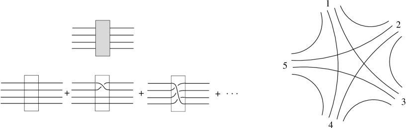
Figure 7: The structure of the propagator and the interaction vertex. Each line represents a delta function as the ones in the integrand of (133) in the case of the propagator and (136) in the case of the vertex. The shaded box in the propagator represents the sum over permutations $\sigma$ in (133). This sum is over diagrams including crossings, we have represented three of this terms in the diagram below the propagator.

There is still a redundant $g_{i}$ integration in (136) which introduces a potentially infinite $vol_{G}$ factor in the vertex amplitude. Notice that the (136) depends on the ‘translational invariant’ combinations $g^{-1}_{i}g_{j}$ so that one of the $g$-integrations is redundant. In other words, one can absorb one of the $g_{i}$ by redefining the remaining four using the invariance of the measure. In the non compact case this would yield another $vol_{G}$ infinite factor. The regularization now consists of removing an arbitrary $g_{i}$ from the expression of the vertex amplitude. This results in the regularization scheme proposed by Barrett and Crane in [10]. The regularization presented here can be applied to any non compact group model on a lattice and can be regarded as a gauge fixing condition for the internal gauge invariance (recall Section 6.1). For notational simplicity we do not implement the regularization explicitly in (136). The structure of the vertex is represented on the left diagram in Fig. 7. Each of the lines represent a delta function appearing in the integrand of (136) (compare with 125).

The Feynman diagrams of the theory are obtained by connecting the $5$-valent vertexes with propagators (see Fig. 7). At the open ends of propagators and vertexes there are the four group variables $x$ corresponding to the arguments of the field (in addition to the integration variables $g_{i}$ and $u_{ij}$ coming from ${\bf P}$ and ${\bf R}$ respectively). For a fixed permutation $\sigma$ in each propagator, one can follow the sequence of delta functions with common arguments across vertexes and propagators. On a closed graph, each such sequence must close. By associating a surface to each such sequence of propagators, we construct a $2$-complex $\cal J$ [11]. Thus, by expanding in Feynman diagrams and in the sum over permutations in (9.1.1), we obtain a sum over 2-complexes. Each 2-complex is given by a certain vertex-propagator topology plus a fixed choice of a permutation on each propagator.

9.1.2 Evaluation in configuration space

Combining (134) and (136) and integrating over internal variables $x_{ij}$ the sequence of delta functions associated to a face $f\in{\cal J}$ reduces to a single delta function. Denoting $v_{1}\dots v_{n}$ the ordered set of $n$ vertices bounding $f$, and $e_{ij}$ the edge connecting $v_{i}$ with $v_{j}$, the delta function corresponding to the face $f$ becomes

$$\delta\left([u^{\scriptscriptstyle f}_{v_{1n}}g^{-1}_{v_{1n}}g_{v_{12}}u^{\scriptscriptstyle f}_{v_{12}}]g_{e_{12}}[u^{\scriptscriptstyle f}_{v_{21}}g^{-1}_{v_{21}}\hat{g}_{v_{23}}u^{\scriptscriptstyle f}_{v_{23}}]g_{e_{23}}\cdots g_{e_{(n-1)n}}[\hat{u}^{\scriptscriptstyle f}_{v_{n(n-1)}}g^{-1}_{v_{n(n-1)}}g_{v_{n1}}u^{\scriptscriptstyle f}_{v_{n1}}]g_{e_{n1}}\right),$$ (137)

where $g_{e_{ij}}\in G$ is the integration variable in (133) associated to the edge $e_{ij}$, $g_{v_{ij}}\in G$ denotes the integration variable in (136) associated with the leg $ij$ of the vertex $v_{i}$ connected to the edge $e_{ij}$, and $u^{\scriptscriptstyle f}_{v_{ij}}\in U$ is the corresponding subgroup integration in one of the delta functions in (136). We use the supra index $f$ to emphasize that the $u$’s appear on single delta functions in (136) and therefore do not contribute to more than one face. In the previous equation, the product of group elements between brackets correspond to the vertex contribution to the face (see (136)) while the $g_{e_{ij}}$ comes from the corresponding propagators (134), also we have that $g_{e_{ij}}=g^{-1}_{e_{ji}}$. Using (137) the amplitude $A({\cal J})$ of an arbitrary closed 2-complex becomes a multiple integral of the form

$$\!\!\!\!\!\!A({\cal J})=\int\prod_{e}dg_{e}\prod_{v}dg_{v}dg_{v}$$ (138)

$$\!\!\!\!\!\!\prod_{f}du^{\scriptscriptstyle f}_{v}du^{\scriptscriptstyle f}_{v}\delta([u^{\scriptscriptstyle f}_{v_{1n}}g^{-1}_{v_{1n}}g_{v_{12}}u^{\scriptscriptstyle f}_{v_{12}}]g_{e_{12}}[u^{\scriptscriptstyle f}_{v_{21}}g^{-1}_{v_{21}}\hat{g}_{v_{23}}u^{\scriptscriptstyle f}_{v_{23}}]g_{e_{23}}\cdots g_{e_{(n-1)n}}[\hat{u}^{\scriptscriptstyle f}_{v_{n(n-1)}}g^{-1}_{v_{n(n-1)}}g_{v_{n1}}u^{\scriptscriptstyle f}_{v_{n1}}]g_{e_{n1}}).$$

Notice that if the subgroup $U=\{\mathbbm{1}\}$ the previous expression coincides with the BF amplitude (67) if we make the change of variables $g^{\prime}_{{e_{ij}}}=g_{v_{ij}}g_{e_{ij}}g^{-1}_{v_{ji}}$. For $U=\{\mathbbm{1}\}$ we recover Ooguri’s GFT [87].

9.1.3 The spin foam representation

The spin foam representation for the amplitude can be obtained by expanding the delta functions in terms of irreducible unitary representations of $G$, namely

$$\delta(g)=\sum_{\rho}\Delta_{\rho}\ {\rm Tr}\left[{\rho}(g)\right],$$ (139)

where $\rho$ labels unitary irreducible representations and the rest of the notation is that of (31) when $G$ is compact. In the non compact case representations are infinite-dimensional so a formally equivalent expression holds where $\Delta_{\rho}$ correspond to the so-called Pancharel measure [112].

Using (139) in (137) the face contribution is

$$\!\!\!\!\!\!\!\!\!\!\!\!\sum_{\rho}\Delta_{\rho}\ {\rm Tr}\left[{\rho}(u^{\scriptscriptstyle f}_{v_{1n}})\cdot\rho(g^{-1}_{v_{1n}}g_{v_{12}})\cdot\rho(u^{\scriptscriptstyle f}_{v_{12}})\cdot{\rho}(g_{e_{12}})\cdot{\rho}(u^{\scriptscriptstyle f}_{v_{21}})\cdot\rho(g^{-1}_{v_{21}}g_{v_{23}})\cdot\right.$$

$$\!\!\!\!\!\!\!\!\!\!\!\!\left.\rho(u^{\scriptscriptstyle f}_{v_{23}})\cdot{\rho}(g_{e_{23}})\cdots{\rho}(u^{\scriptscriptstyle f}_{v_{n(n-1)}})\cdot\rho(g^{-1}_{v_{n(n-1)}}g_{v_{n1}})\cdot\rho(u^{\scriptscriptstyle f}_{v_{n1}})\cdot{\rho}(g_{e_{n1}})\right],$$ (140)

where we have dropped the integration symbols for simplicity. The $u$’s appear just once per face so we can perform the $u$-integrations independently of other faces. Notice that $\int du\rho(u)$ is the projection onto the invariant subspace under the action of $U$ in the Hilbert space ${\cal H}_{\rho}$. When $U=\{\mathbbm{1}\}$ the projector is the identity. In the other cases the subspace turns out to be 1-dimensional. Consequently the projector can be written as

$$\int\limits_{U}du\ \rho(u)=\left|w_{\scriptscriptstyle\rho}\right>\left<w_{\scriptscriptstyle\rho}\right|,$$ (141)

where $\left|w_{\scriptscriptstyle\rho}\right>$ is the corresponding invariant vector. Equation (9.1.3) becomes

$$\sum_{\rho}\Delta_{\rho}\ \left<w_{\scriptscriptstyle\rho}\right|\rho(g^{-1}_{v_{1n}}g_{v_{12}})\left.w_{\scriptscriptstyle\rho}\right>\left<w_{\scriptscriptstyle\rho}\right|{\rho}(g_{e_{12}})\left.w_{\scriptscriptstyle\rho}\right>\left<w_{\scriptscriptstyle\rho}\right|\rho(g^{-1}_{v_{21}}g_{v_{23}})\left.w_{\scriptscriptstyle\rho}\right>\cdots\left<w_{\scriptscriptstyle\rho}\right|{\rho}(g_{e_{n1}})\left.w_{\scriptscriptstyle\rho}\right>.$$ (142)

There are two types of terms in the previous equation: those corresponding to edges for which the representation $\rho$ is evaluated at the single $g_{e_{ij}}$ group variable, and those corresponding to vertices for which $\rho$ is evaluated at the product $g^{-1}_{v_{ij}}g_{v_{ik}}$. Let us integrate over the edge variables first. The group element $g_{e}$ associated to an edge $e\in{\cal J}$ appears four times as there are four delta functions in the propagator (134). Therefore, integrals over such $g$’s have the general form

$$A_{e}(\rho^{1}_{e},\dots,\rho^{4}_{e})=\int\limits_{G}\left<w_{\scriptscriptstyle\rho^{1}}\right|{\rho^{1}}(g)\left.w_{\scriptscriptstyle\rho^{1}}\right>\left<w_{\scriptscriptstyle\rho^{2}}\right|{\rho^{2}}(g)\left.w_{\scriptscriptstyle\rho^{2}}\right>\left<w_{\scriptscriptstyle\rho^{3}}\right|{\rho^{3}}(g)\left.w_{\scriptscriptstyle\rho^{3}}\right>\left<w_{\scriptscriptstyle\rho^{4}}\right|{\rho^{4}}(g)\left.w_{\scriptscriptstyle\rho^{4}}\right>,$$ (143)

and define the edge amplitude. If we define the kernel $K_{\rho}(g)$ as

$$K_{\rho}(g)\equiv\left<w_{\scriptscriptstyle\rho}\right|{\rho}(g)\left.w_{\scriptscriptstyle\rho}\right>,$$ (144)

then using the subgroup invariance of the $\left|w_{\scriptscriptstyle\rho}\right>$’s the previous equation becomes

$$A_{e}(\rho_{1},\dots,\rho_{4})=vol_{U}\times\int\limits_{G/U}dy\ K_{\rho_{1}}(y)K_{\rho_{2}}(y)K_{\rho_{3}}(y)K_{\rho_{4}}(y),$$ (145)

where the integration is over the homogeneous space $G/U$. Integration over the group elements associated to vertices are of the general form

$$A_{v}(\rho_{ik})=\int\limits_{(G/U)^{4}}\prod\limits_{i=1}^{5}dy_{i}\ \prod\limits_{i<k}K_{\scriptscriptstyle\rho_{ik}}(y_{i},y_{k}).$$

This corresponds to the vertex amplitude. When $U$ is non compact the preceding expressions have to be regularized as in Subsection 9.1.1 by dropping an arbitrary $y$-integration. The amplitude of a 2-complex ${\cal J}$ is then given by

$$A({\cal J})=\sum\limits_{{\cal C}_{f}:\{f\}\rightarrow\{\rho\}}\prod_{f\in{\cal J}}\Delta_{\rho_{f}}\prod_{e\in{\cal J}}A_{e}(\rho_{1},\dots,\rho_{4})\prod_{v\in{\cal J}}A_{v}(\rho_{1},\dots,\rho_{10})$$ (146)

As we shall see in the following the presence of ${\bf R}$ in (128) can be interpreted as imposing the Barrett-Crane constraints on the GFT dual to BF theory.

9.1.4 Boundaries

The amplitude of an open diagram, that is, a diagram with a boundary, is a function of the variables on the boundary, as for conventional QFT Feynman diagrams. The boundary of a 2-complex is given by a graph. To start with, the amplitude of the open diagram is a function of 4 group arguments per each external leg. However, consider a surface of an open 2-complex and the link $ab$ of the boundary graph that bounds it. Let $a$ and $b$ be the nodes on the boundary graph that bounds $ab$. The surface determines a sequence of delta functions that starts with one of the group elements in $a$, say $g_{a}$, and ends with one of the group elements in $b$, say $g_{b}$. By integrating internal variables, all these delta functions can be contracted to a single one of the form $\delta(g_{a}\cdots g_{b}^{-1})=\delta(g_{b}^{-1}g_{a}\cdots)$. We can thus define the group variable $\rho_{ab}=g_{b}^{-1}g_{a}$, naturally associated to the link $ab$, and conclude that the amplitude of an open 2-complex is a function $A(\rho_{ab})$ of one group element per each link of its boundary graph. $A(\rho_{ab})$ is gauge invariant as can be easily checked, and $\rho_{ab}$ represents the discrete boundary connection in the language of Section 3.2.

In “momentum space”, boundary degrees of freedom are encoded in spin-network states. That is, if $s$ is a spin network given by a coloring of the boundary graph, then

$$A(s)=\int d\rho_{ab}\ \bar{\psi}_{s}(\rho_{ab})\ A(\rho_{ab}),$$ (147)

where $\psi_{s}(\rho_{ab})$ is the spin network function [26, 27]. The formula can be inverted

$$A(\rho_{ab})=\sum_{s}A(s)\psi_{s}(\rho_{ab}),$$ (148)

where the sum is performed over all spin network states defined on the given boundary graph. The argument presented here applies in general for any GFT of the kind introduced in Section 8. In the case of the GFT’s defined here $\rho_{ab}=g_{b}^{-1}g_{a}$ will appear between $U$-integrations. So strictly speaking, for each $\rho_{ab}=g_{b}^{-1}g_{a}$ there correspond two point $y_{a}$ and $y_{b}$ in the homogeneous space $G/U$ and one cannot say that the amplitude depend on the $G$-connection.

9.2 GFT dual to the Riemannian Barret-Crane model

The representation theory of $Spin(4)$ is particularly simple due to the fact that $Spin(4)=SU(2)\times SU(2)$. Unitary irreducible representations of $\rho$ of $Spin(4)$ are labeled by two half-integers $j_{l}$ and $j_{r}$, and are given by the tensor product of unitary irreducible representations of SU(2), namely

$$\rho_{j_{l}j_{r}}=j_{l}\otimes j_{r}.$$ (149)

In terms of representation matrices we have

$$R^{j_{l}j_{r}}(g)_{mm^{\prime}qq^{\prime}}=D^{j_{l}}_{mm^{\prime}}(g_{r})D^{j_{r}}_{qq^{\prime}}(g_{l}),$$ (150)

where $g=(g_{l},g_{r})\in Spin(4)$, and $D^{j_{l}}_{mm^{\prime}}$ are $SU(2)$-representation matrices. The subgroup $U$ of previous section is taken as $U=SU(2)\subset Spin(4)$ defined by the diagonal action on $Spin(4)$ as follows

$$gu\equiv(g_{l}u,g_{r}u)\ \ \ {\rm for}\ \ \ u\in U.$$ (151)

The projector (141) can be explicitly evaluated

$$\int\limits_{U}du\ \rho_{j_{l}j_{r}}(u)=\int du\ D^{j_{l}}_{mm^{\prime}}(u)D^{j_{r}}_{qq^{\prime}}(u)=\frac{\delta_{j_{l}j^{*}_{r}}}{2j_{l}+1}\delta_{mq}\delta_{m^{\prime}q^{\prime}}=\left|w_{\scriptscriptstyle j_{l}}\right>\left<w_{\scriptscriptstyle j_{l}}\right|,$$ (152)

where we have used the orthonormality of $SU(2)$ representation matrices (Footnote 10). The previous equation confirms that the invariant subspace for each $\rho_{j_{l}j_{r}}$ is 1-dimensional as anticipated above. An immediate consequence of (152) is that the kernel $K_{\rho}$ in (144) becomes

$$K_{j}(g)=\left<w_{\scriptscriptstyle j}\right|{\rho_{j^{\prime}j}}(g)\left.w_{\scriptscriptstyle j}\right>=\frac{\delta_{j^{\prime}j^{*}}}{{2j+1}}{\rm Tr}\left[D^{j}(g_{l}g_{r})\right].$$ (153)

The factor $\delta_{j^{\prime}j}$ restricts the representation to the simple representations $j_{l}=j^{*}_{r}=j$.

The projector ${\bf R}$ in (128) imposes the Barrett-Crane simplicity constraints of equation (7.3)!. Simple representations appear in the harmonic analysis of functions on the 3-sphere, $S_{3}$. The fact that we encounter them here is not surprising since $S_{3}$ is the homogeneous space $S_{3}=Spin(4)/SU(2)$ under the $SU(2)$ diagonal insertion (151). The presence of $R$ in (128) projects out those modes that are not simple or spherical. Indeed, $\left<w_{\scriptscriptstyle j}\right|{\rho_{j^{\prime}j^{*}}}(g)\left.w_{\scriptscriptstyle j}\right>$ can be thought of as a function on $S_{3}$: $\left<w_{\scriptscriptstyle j}\right|{\rho_{j^{\prime}j^{*}}}(g)\left.w_{\scriptscriptstyle j}\right>$ depends on the product $g_{l}g_{r}\in SU(2)$ which is isomorphic to $S_{3}$. We will see below that in fact ${\bf R}$ imposes all the constraints of Section 7.3 fixing in addition the value of the so far undetermined edge amplitude $A_{e}$.

The invariant measure on $SU(2)$ can be written as a measure on $S_{3}$ induced by the isomorphism $SU(2)\rightarrow S_{3}$. We can parameterize $h\in SU(2)$ as $h=y_{\scriptscriptstyle(h)}^{\mu}\tau_{\mu}$ where $\tau_{k}=i\sigma_{k}$ for $k=1,2,3$, $\{\sigma_{k}\}$ is the set of Pauli matrices, and $\tau_{0}=1$. $h\in SU(2)$ implies $y_{\scriptscriptstyle(h)}^{\mu}y_{{\scriptscriptstyle(h)}{\mu}}=1$ (indexes are lowered and raised with $\delta^{\mu}_{\nu}$), i.e., $y\in S_{3}$. In this parameterization the $SU(2)$ Haar measure becomes

$$dh\rightarrow dy=\frac{1}{\pi^{2}}dy^{\scriptscriptstyle 4}\delta(y^{\mu}y_{\mu}-1),$$ (154)

We can simplify the measure using spherical coordinates for which an arbitrary point $y\in S^{3}$ is written

$$y=\left({\rm cos}(\psi),{\rm sin}(\psi){\rm sin}(\theta){\rm cos}(\phi),{\rm sin}(\psi){\rm sin}(\theta){\rm sin}(\phi),{\rm sin}(\psi){\rm cos}(\theta)\right),$$ (155)

where $0\leq\psi\leq\pi$, $0\leq\theta\leq\pi$, and $0\leq\phi\leq 2\pi$. The Haar measure becomes

$$dy=\frac{1}{2\pi^{2}}\ {\rm sin}^{2}(\psi)\,{\rm sin}(\theta)\ d\psi\,d\theta\,d\phi.$$ (156)

Using the known formula for the trace of $SU(2)$ representation matrices it is easy to check that (153) becomes

$$K_{j}(\psi_{y})=\frac{\delta_{j^{\prime}j}}{{2j+1}}\frac{{\rm sin}((2j+1)\psi_{y})}{{\rm sin}(\psi_{y})},$$ (157)

where $\psi_{h}$ is the value of the coordinate $\psi$ in (155) corresponding to $y\in SU(2)$. Notice that we have rediscovered the kernel (103) which together with equation (104) establishes the claimed duality between the Barrett-Crane model and the GFT of this section.

Now, the general edge and vertex amplitudes ((145) and (9.1.3)) reduce to multiple integrals over $S_{3}$. These can be interpreted as the evaluation of diagrams on the sphere with propagator given by (157). This evaluation is referred to as relativistic spin network evaluation in the literature. In the case of the edge amplitude the evaluation corresponds to a $\theta_{4}$ graph with four links labeled by the four spins $j_{1},\dots,j_{4}$. In the case of the vertex amplitude the evaluation corresponds to the $\gamma_{5}$ spin network of Figure 4 for which the ten links are labeled by the corresponding ten spins $j_{1},\dots,j_{10}$. There is no intertwiner label at nodes as the projection ${\bf R}$ fixes the intertwiners to the unique Barrett-Crane one.

The amplitude $A_{e}(j_{1},\dots,j_{4})$ can be computed using (153) and (33), it follows that

$$A_{e}(j_{1},\dots,j_{4})=\frac{{\rm dim}\left[{\rm Inv}({j_{1}}\otimes{j_{2}}\otimes{j_{3}}\otimes{j_{4}})\right]}{{\rm dim}\left[{j_{1}}\otimes{j_{2}}\otimes{j_{3}}\otimes{j_{4}}\right]},$$ (158)

where ${\rm dim}\left[{\rm Inv}({j_{1}}\otimes{j_{2}}\otimes{j_{3}}\otimes{j_{4}})\right]$ denotes the dimension of the trivial component of ${\cal H}_{j_{1}}\otimes{\cal H}_{j_{2}}\otimes{\cal H}_{j_{3}}\otimes{\cal H}_{j_{4}}$ and ${\rm dim}\left[{j_{1}}\otimes{j_{2}}\otimes{j_{3}}\otimes{j_{4}}\right]$ the dimension of the full space. So finally,

$$A({\cal J})=\sum\limits_{{\cal C}_{f}:\{f\}\rightarrow\{j\}}\prod_{f\in{\cal J}}(2j_{f}+1)^{2}\prod_{e\in{\cal J}}A_{e}(j_{1},\dots,j_{4})\prod_{v\in{\cal J}}A_{v}(j_{1},\dots,j_{10}),$$ (159)

where the vertex amplitude is given by (9.1.3) using (157). This is the Barrett-Crane model (98) where the values of $A_{e}$ and $A_{f}$ have been fixed by the GFT formulation.

9.2.1 Finiteness

In this section we prove that the infinite spin sum in (159) is convergent if the $2$-complex ${\cal J}$ is finite and non-degenerate. In order to do this we need to construct bounds for the terms in the sum (edge and vertex amplitudes). These bounds are provided by the following lemmas.

Lemma 9.1.

[18] For any subset of $\kappa$ elements $j_{1}\dots j_{\kappa}$ out of the corresponding four representations appearing in $A_{e}(j_{1},\dots,j_{4})$, the following bounds hold:

$$\left|A_{e}(j_{1},\dots,j_{4})\right|\leq\frac{1}{\prod\limits^{\kappa}_{i=1}(2j_{i}+1)^{\alpha_{\kappa}}},\ \ \ {where}\ \ \ \alpha_{\kappa}=\left\{\begin{array}[]{ccc}1\ \ {for}\ \ \kappa\leq 3\\ \frac{3}{4}\ \ {for}\ \ {k=4}\end{array}\right..$$

The inequality for $\kappa\leq 3$ is sharp.

The proof of this lemma is elementary and can be found in [18].

Lemma 9.2.

[18] For any $4$ spins $j_{1}\dots j_{4}$ labeling links converging at the same node in the relativistic spin-network corresponding to $A_{v}(j_{1},\dots,j_{10})$ the following bounds hold:

$$\left|A_{v}(j_{1},\dots,j_{10})\right|\leq\frac{1}{(2j_{1}+1)(2j_{2}+1)(2j_{3}+1)(2j_{4}+1)},$$

from which follows

$$\left|A_{v}(j_{1},\dots,j_{10})\right|\leq\frac{1}{((2j_{1}+1)\dots(2j_{10}+1))^{2/5}}.$$

Definition 9.1.

A 2-complex ${\cal J}$ is said to be degenerate if it contains some faces bounded by only one or two edges.

Theorem 9.1.

[18] The state sum $A({\cal J})$, (159), converges for any non degenerate 2-complex ${\cal J}$.

Proof.

The amplitude (159) can be bounded in the following way:

$$|A({\cal J})|\leq\prod_{f\in{\cal J}}\sum_{j_{f}}\left((2j_{f}+1)\right)^{2-\frac{3}{4}n_{f}-\frac{4}{10}n_{f}}=\prod_{f\in{\cal J}}\sum_{j_{f}}\left((2j_{f}+1)\right)^{2-\frac{23}{20}n_{f}},$$ (160)

where $n_{f}$ denotes the number of edges of the corresponding face, and we have used the fact the number of edges equals the number of vertices in a face of ${\cal J}$. The term $(2j+1)^{2}$ in (160) comes from the face amplitude, $(2j+1)^{-\frac{3}{4}n_{f}}$ from Lemma 9.1 ($\kappa=4$), and $(2j+1)^{-\frac{4}{10}n_{f}}$ from Lemma (9.2) $\kappa=10$. Notice that if the 2-complex contains faces with more than two edges the previous bound for the amplitude is finite, since the sum on the RHS of the previous equation converges for $n_{f}>2$. ∎

The fact that the sum over spins converges for a fixed (non degenerate) $2$-complex is an very encouraging result. It means that for a fixed $2$-complex the sum over the infinite set of $4$-geometry configurations, represented by the corresponding spin foams, is well defined. Even though the result was obtained in the context of the GFT formulation, it can be applied to the model defined on a simplicial decomposition of the space-time manifold. This is because (159) refers to the amplitude of a single Feynman diagram. In this context, the result is very encouraging and appears as a first necessary step for the construction of the discretization independent generalized projector and physical scalar product by studying the refinement limit of Section 6.2. On the other hand, if the discretization independent formulation is to be obtained directly by means of the GFT formulation, this result means that the perturbative expansion in $\lambda$ (116) is finite order by order. The previous statement has not been completely proved as degenerate $2$-complexes—for which our proof does not hold—will appear in the $\lambda$-expansion. However, we expect these diagrams to be finite also. A proof of this is lacking at the moment but it should be feasible by strengthening the bounds we have used in this section.

9.3 Lorentzian models

Unitary irreducible representations of $SL(2,{\mathbb{C}})$ appearing in the general expression (139) are the ones in the so-called principal series. They are labeled by a natural number $n$ and a positive real number $\rho$. Unitary irreducible representations of $SL(2,{\mathbb{C}})$ are infinite dimensional. Those in the principal series are defined by their action on the linear space ${\cal D}_{n\rho}$ of homogeneous functions of degree $(\frac{n+i\rho}{2}-1,\frac{-n+i\rho}{2}-1)$ of two complex variables $z_{1}$ and $z_{2}$. Due to the homogeneity properties of the elements ${\cal D}_{n\rho}$ they can be characterized by giving their value on the sphere $|z_{1}|^{2}+|z_{2}|^{2}=1$. The latter is isomorphic to $SU(2)$. The so called canonical basis is defined in terms of functions on $SU(2)$ and is well suited for studying the following model. The relevant facts about $SL(2,{\mathbb{C}})$ representation theory and the notation used in this section can be found in the appendix of reference [112] (for all about $SL(2,{\mathbb{C}})$ representation theory see [119]).

9.3.1 GFT dual to the Lorentzian Barrett-Crane model

Equation (141) becomes, in this case,

$$\int\limits_{U}du\ \rho_{n\rho}(u)=\int\limits_{SU(2)}duD^{n\rho}_{\ell m\ell^{\prime}m^{\prime}}(u)=\delta_{n0}\delta_{\ell 0}\delta_{\ell^{\prime}0}=\left|w_{\scriptscriptstyle n\rho}\right>\left<w_{\scriptscriptstyle n\rho}\right|,$$ (161)

in terms of the canonical basis [112]. The $SU(2)$ invariant vectors $\left|w_{\scriptscriptstyle n\rho}\right>$ are given by $\left<z_{1},z_{2}\right.\left|w_{\scriptscriptstyle n\rho}\right>=\delta_{n0}(|z_{1}|^{2}+|z_{2}|^{2})^{\frac{i}{2}\rho-1}$ which is indeed a homogeneous function of degree $(\frac{i\rho}{2}-1,\frac{i\rho}{2}-1)$.

An immediate consequence of (161) is that the kernel $K_{\rho}$ in (144) becomes

$$K_{n\rho}(g)=\left<w_{n\rho}\right|{\rho_{n\rho}}(g)\left.w_{\scriptscriptstyle n\rho}\right>=\delta_{n0}D^{n\rho}_{0000}(u).$$ (162)

The kernel $\left<w_{\scriptscriptstyle 0\rho}\right|{\rho_{0\rho}}(g)\left.w_{\scriptscriptstyle 0\rho}\right>$ can be thought of as a function on $H^{+}=SL(2,{\mathbb{C}})/SU(2)$ (the upper sheet of $2$-sheeted hyperboloid in Minkowski space). An arbitrary point $y\in H^{+}$ can be written in hyperbolic coordinates as

$$y=\left({\rm cosh}(\eta),{\rm sinh}(\eta){\rm sin}(\theta){\rm cos}(\phi),{\rm sinh}(\eta){\rm sin}(\theta){\rm sin}(\phi),{\rm sinh}(\eta){\rm cos}(\theta)\right),$$ (163)

where $0\leq\eta\leq\infty$, $0\leq\theta\leq\pi$, and $0\leq\phi\leq 2\pi$. The invariant measure in these coordinates is

$$dy=\frac{1}{2\pi^{2}}\ {\rm sinh}^{2}(\eta)\,{\rm sin}(\theta)\ d\eta\,d\theta\,d\phi.$$ (164)

In these coordinates, (162) becomes

$$K_{{\rho}}(\eta_{y})=\frac{2}{{\rho}}\frac{{\rm sin}(\frac{1}{2}\rho\eta_{y})}{{\rm sinh}(\eta_{y})},$$ (165)

where $\eta_{y}$ is the value of the coordinate $\eta$ corresponding to $y\in H^{+}$ (this the generalization of (103) proposed in [10]). Finally, the amplitude of an arbitrary diagram (146) becomes

$$A(J)=\int\limits_{{\cal C}_{f}:\{f\}\rightarrow\{{\rho}\}}\prod_{f\in J}\rho_{f}^{2}d\rho_{f}\prod_{e\in J}A_{e}(\{{\rho}_{e}\})\prod_{v\in J}A_{v}(\{{\rho}_{v}\}),$$ (166)

where the formal sum in the general expression (146) becomes a multiple integral over the coloring ${\cal C}_{f}:\{f\}\rightarrow\{{\rho}\}$ of faces, and the weight $\Delta_{\rho}$ now is given by the Pancherel measure, $\rho^{2}d\rho$, of $SL(2,{\mathbb{C}})$. The vertex amplitude was proposed in [10], the full state sum amplitude including the previous normalization was obtained in [13].

9.3.2 Finiteness

The amplitude of a non degenerate 2-complex turns out to be finite as in the Euclidean case. We state and prove the main result. Some of the following lemmas are stated without proof; the reader interested in the details is referred to the references. As in the Riemannian case the main idea is to construct appropriate bounds for the fundamental amplitudes.

Lemma 9.3.

[19, 20] For any subset of $\kappa$ elements $\rho_{1}\dots\rho_{\kappa}$ out of the corresponding four representations appearing in $A_{e}({\rho}_{1},\dots,{\rho}_{4})$, the following bounds hold:

$$\left|A_{e}({\rho}_{1},\dots,{\rho}_{4})\right|\leq\frac{C_{\kappa}}{\left(\prod\limits^{\kappa}_{i=1}\rho_{i}\right)^{\alpha_{\kappa}}},\ \ \ {where}\ \ \ \alpha_{\kappa}=\left\{\begin{array}[]{ccc}1\ \ {for}\ \ \kappa\leq 3\\ \frac{3}{4}\ \ {for}\ \ {k=4}\end{array}\right..$$

for some positive constant $C_{\kappa}$.

Lemma 9.4.

[120] $A_{e}({\rho}_{1},\dots,{\rho}_{4})$ and $A_{v}({\rho}_{1},\dots,{\rho}_{10})$ are bounded by a constant independent of the $\rho$’s.

Lemma 9.5.

[19, 20] For any subset of $\kappa$ elements $\rho_{1}\dots\rho_{\kappa}$ out of the corresponding ten representations appearing in $A_{v}({\rho}_{1},\dots,{\rho}_{10})$ the following bounds hold:

$$\left|A_{v}({\rho}_{1},\dots,{\rho}_{10})\right|\leq\frac{K_{\kappa}}{\left(\prod\limits^{\kappa}_{i=1}\rho_{i}\right)^{\frac{3}{10}}}$$

for some positive constant $K_{\kappa}$.

Theorem 9.2.

[19, 20] The state sum $A({\cal J})$, (166), converges for any non degenerate 2-complex ${\cal J}$.

Proof.

We divide each integration region ${\mathbb{R}}^{+}$ into the intervals $[0,1)$, and $[1,\infty)$ so that the multiple integral decomposes into a finite sum of integrations of the following types:

1. All the integrations are in the range $[0,1)$. We denote this term $T(F,0)$, where $F$ is the number of 2-simplexes in the triangulation. This term in the sum is finite by Lemma 9.4.

2. All the integrations are in the range $[1,\infty)$. This term $T(0,F)$ is also finite since, using Lemmas 9.3 and 9.5 for $\kappa=4$, and $\kappa=10$ respectively, we have

   $$T(0,F)\leq\prod_{f}\int\limits^{\infty}_{\rho_{f}=1}d\rho_{f}\ \ \rho_{f}^{2-\frac{3}{4}{n_{e}}-\frac{3}{10}{n_{v}}}\leq\left(\ \int\limits^{\infty}_{\rho_{f}=1}d\rho_{f}\ \ \rho_{f}^{-\frac{46}{40}}\right)^{F}<\infty.$$

3. $m$ integrations in $[0,1)$, and $F-m$ in $[1,\infty)$. In this case $T(m,F-m)$ can be bounded using Lemmas (9.3) and (9.5) as before. The idea is to choose the appropriate subset of representations in the bounds (and the corresponding values of $\kappa$) so that only the $m-F$ representations integrated over $[1,\infty)$ appear in the corresponding denominators. Since this is clearly possible, the $T(m,F)$ terms are all finite.

We have bounded ${\cal Z}$ by a finite sum of finite terms which concludes the proof. ∎

The ‘scaling’ behavior of amplitudes in the model is very similar to that of the Riemannian version of the previous section. If one makes the substitution $(2j+1)=-i\rho$ and $\psi_{y}=i\eta_{y}$ in the Riemannian expression for the kernel (157) one obtains the Lorentzian expression (165). In addition, with the same substitution the face amplitude $(2j+1)^{2}$ in (159) takes the form $\rho^{2}$ of the face amplitude in (166). From this viewpoint the finiteness of the Lorentzian model is intimately related to the finiteness of the Riemannian counterpart.

The non compactness of $SL(2,{\mathbb{C}})$ introduces potential divergences due to the fact that $vol_{SL(2,{\mathbb{C}})}=\infty$. This problem can be dealt with in the GFT formulation by using the appropriate gauge fixing conditions as explained in Section 9. If we define the model on a simplicial decomposition the same gauge fixing can be implemented.

9.3.3 A new Lorentzian model

In the Euclidean case there was only one way of selecting the subgroup $U$ of group elements leaving invariant a fixed direction in Euclidean space-time. In the Lorentzian case there are two possibilities. The case in which that direction is space-like was treated in the previous section. When the direction is time-like the relevant subgroup is $U=SU(1,1)\times{\mathbb{Z}}_{2}$.

This case is more complicated due to the non-compactness of $U$. Consequently, one has to deal with additional infinite volume factors of the form $U$-volume in (129). Another consequence is that the invariant vectors defined in (141) are now distributional and therefore no longer normalizable. All this makes more difficult the convergence analysis performed in the previous models and the issue of finiteness remains open.

On the other hand, the model is very attractive as its state sum representation contains simple representations in both the continuous and discrete series. As pointed out in [10] and discussed in the following section one would expect both types of simple representations to appear in a model of Lorentzian quantum gravity.

The difficulties introduced by the non-compactness of $U$ make the calculation of the relevant kernels (144) more involved. No explicit formulas are known and they are defined by integral expressions. We will not derive these expressions here. A complete derivation can be found in [112]. The idea is to use harmonic analysis on the homogeneous space $SL(2,{\mathbb{C}})/SU(1,1)\times{\mathbb{Z}}_{2}$ which can be realized as the one-sheeted hyperboloid $y^{\mu}y^{\nu}\eta_{\mu\nu}=-1$ where $y$ and $-y$ are identified (imaginary Lobachevskian space, from now on denoted $H^{-}$). The kernels correspond to eigenfunctions of the massless wave equation on that space.

The corresponding kernel is given by the following expression:

$$K_{\rho,n}(x,y) = \int\limits_{C^{+}}d\omega(\delta_{n,0}\left|y^{\nu}\xi_{\nu}\right|^{i\frac{\rho}{2}-1}\left|x^{\nu}\xi_{\nu}\right|^{-i\frac{\rho}{2}-1}$$ (167)

$$+ \delta(\rho)\delta_{n,4k}\frac{32\,\pi e^{-2ik\left[\Theta(x,y)\right]}}{k}\ \delta(x^{\nu}\xi_{\nu})\delta(y^{\nu}\xi_{\nu})),$$

where $x,y\in H^{-}$ and $\xi\in C^{+}$ is a normalized future pointing null vector in Minkowski space-time. The integration is performed on the unit sphere defined by these vectors with the standard invariant measure $d\omega$.

As in the previous cases the expressions for the edge and vertex amplitudes (equations (145) and (9.1.3)) reduce to integrals on the hyperboloid $H^{-}$. The expression for the amplitude (146) of an arbitrary diagram is [112]

$$A(J)=\sum_{n_{f}}\int\limits_{\rho_{f}}d\rho_{f}\prod_{{f}}\ (\rho_{f}^{2}+n^{2}_{f})\ \prod_{{e}}\ A_{e}(\{n_{e}\},\{\rho_{e}\})\ \prod_{{v}}\ A_{v}(\{n_{v}\},\{\rho_{v}\}),$$

where now there is a summation over the discrete representations $n$ and an multiple integral over the continuous representations $\rho$. For the discrete representations the triangle area spectrum takes the form (107) if we define $k=j+1/2$. The finiteness properties of this model have not been studied so far. There is a relative minus sign between the continuous and discrete eigenvalues of the area squared operators that has been interpreted as providing a notion of micro causality in [112]. It would be interesting to study this in connection with the models of Section 5.5.

10 Discussion

We conclude this article with some remarks and a discussion of recent results and future perspectives in the subject. As we have devoted the second part of this paper almost exclusively to the Barrett-Crane model we start by discussing open issues in this context. We go to more general open questions toward the end of this section.

$1$. Normalization: The Barrett-Crane model is certainly the most well studied spin foam model for $4$-dimensional quantum gravity. However, as we pointed out at the end of Section 7, the definition of the measure is incomplete since there remains to determine the value of lower dimensional simplex amplitudes such as the edge (tetrahedron) amplitude $A_{e}$. Although, the normalization (158, 159) of the Barrett-Crane model can be fixed in a natural way using the GFT formulation—or using similar (subgroup averaging) arguments [118, 121, 122]—one would really like to understand this prescription in relation to the continuum theory.

In Section 7, we have shown that the Barrett-Crane model can in fact be interpreted as a ‘lattice’ formulation of the gravity sector of the $SO(4)$ Plebanski theory—this conclusion can be extended to the Lorentzian theory without further complications. This close relationship between the model and a continuum action suggested the possibility of determining the correct spin foam measure by comparison with the formal continuum path phase space path integral measure of Plebanski’s theory. If the value of the edge amplitude (158) could be found in this way this would provide further evidence for the GFT-gravity duality and strengthen the finiteness results. These considerations apply also for other spin foam models in particular to those defined by constraining BF theory. A general prescription for the construction of an anomaly free measure for spin foam models is investigated in [85].

$2$. Numerical results: A very attractive property of the normalization (159) is however the finiteness of transition amplitudes on a fixed discretization. Having a well defined model—for both Riemannian and Lorentzian gravity—has opened for the first time the possibility for numerical explorations. An important step toward the numerical evaluation of the BC model is the development of efficient algorithms for the computation of the $10j$-symbols [123]. Numerical calculations by Baez et al. [93] show that the sum over spin foams in our normalization of the Barrett-Crane model converges very fast so that amplitudes are dominated by spin foams where most of the faces are labeled by zero spin. The leading contribution comes from spin foams made up from isolated ‘bubbles of geometry’. This problem is however not present in the Lorentzian version (166) where simple representations are in the continuum part of the spectrum. Baez, Christensen, Halford and Tsang propose modifications of the normalization which still yield finite amplitudes but avoid this puzzling feature. However, these modifications consist of ad hoc definitions of the value of edge and face amplitudes. A clear understanding of this would have to come with the understanding of the normalization issues discussed above.

If we take seriously the normalization (158), the previous result might not be so worrisome after all. According to Section 7.6, the asymptotic expression of the vertex amplitude shows that for large spins it is dominated by degenerate $4$-simplexes. These configurations are however strongly suppressed by the form of the edge amplitude (158) in our normalization. Assuming that for small spin values the amplitudes behave appropriately, large spin behavior might not be physically relevant after all.

As pointed out by Smolin [124], one could neglect spin zero representations according to the argument that they represent ‘zero geometry states’ (all geometric operators vanish on the spin zero subspace). If one does so, then transition amplitudes are dominated by the spin one half representations and the model becomes very similar to a model of dynamical triangulations—in dynamical triangulations one sums over triangulations whose $1$-simplexes have the same definite length, while here the amplitudes are dominated by triangulations where triangles have the same fixed area given by (107) for $j=1/2$. However one should also point out an important difference: in our case, configurations are weighted with complex amplitudes ${\rm exp}(iS)$ which no (a priori) connection to the Euclidean amplitude ${\rm exp}(-S)$ of dynamical triangulations. In the Lorentzian models the analogy simply disappears as representation labels are continuous.

$3$. The connection with the canonical picture: We began this article motivating the spin foam approach from the perspective of loop quantum gravity. Can we establish a rigorous connection between the spin foam models presented here and the canonical formulation? In all the models (for Riemannian gravity) introduced in Section 5, with the exception of the Barrett-Crane model, this relationship is manifest at the kinematical level as the boundary states are given by $SU(2)$-spin networks. This kinematic connection exists by construction in these cases.

What happens in the case of the Barrett-Crane model? The Riemannian BC model is defined in terms of $Spin(4)$, so naturally one could expect the boundary data to be given by $Spin(4)$ spin networks (labeled by two half-integers $(j_{\ell},j_{r})$). The simplicity constraints impose $j_{\ell}=j_{r}=j$ which could be interpreted as the existence of an underlying $SU(2)$ connection. However, it can be shown that the boundary data of the model cannot be interpreted as given by an $SU(2)$ connection (recall the discussion of Section 9.1.4). Similarly, in the Lorentzian Barrett-Crane model boundary states could be naively related to $SL(2,{\mathbb{C}})$ spin networks. However similar considerations as in the Riemannian sector show that the simplicity constraints (applied à la Barrett-Crane) reduce the boundary states in a way that cannot be interpreted as a boundary connection. Alexandrov [125, 126] has been studying the possibility of defining a $SL(2,{\mathbb{C}})$ connection canonical formulation of general relativity. The second class constraints of the theory—related to the simplicity constraints of Plebanski’s formulation—are dealt with using the Dirac bracket in terms of which the original connection becomes non commutative. In this sense there is no genuine or standard spin network representation of states. It seems that such approach could lead to the understanding of the relationship of the Barrett-Crane model and a canonical formulation of gravity. The are in fact some indications of this [127, 128].

Another difficulty in making contact with LQG is the fact that operators associated to triangle-areas have continuous spectrum in the Lorentzian models which is in conflict with the canonical result (7). From this perspective one is compelled to study the model we have described in Section 9.3.3 for which part of the area spectrum coincides with (7).

In the canonical framework the compact $SU(2)$ formulation is achieved by means of the introduction of the Imirzi parameter $\iota$ which defines a one parameter family of unitarily inequivalent representations of quantum gravity. In particular, geometric operators are modulated by $\iota$ (see (7) for example). Can the spin foam approach say something about $\iota$? There is no conclusive answer to this question so far. The spin foam quantization of generalizations of Plebanski’s action including the $\iota$ ambiguity [129] are analyzed in [130, 131].

So far we have only compared spin foams with loop quantum gravity at the kinematical level. However, one of the main motivations of the approach was the expected simplification in addressing dynamical questions. As we mentioned before, dynamics is not well understood in the canonical formulation. This is mostly due to the difficulties associated to regularization ambiguities in the construction of the scalar constraint, the understanding of its space of solutions and the the definition of the physical scalar product. As we have seen all these issues can be naturally addressed in the spin foam formulation. In turn, it would be nice to understand whether the approach can help set a guiding principle that would allow for the selection of a preferred regularization of the scalar constraint. Understanding of this question would strengthen the relationship between the two formulations. An explicit analysis of the relation between the covariant (spin foam) and canonical formulation of BF theory is presented in [132]. The reconstruction of the corresponding scalar constraint operator is studied and carried out explicitly in simple models.

$4$. Alternatives to the Barrett-Crane model: The fact that degenerate configurations dominate the asymptotics of the Barrett-Crane vertex amplitude [109] can be interpreted as a serious problem. A possible solution to the apparent problem is proposed in [110], where the evaluation of the vertex amplitude is modified in a simple way to avoid degenerate contributions. The potential dominance of degenerate sectors of Plebanski’s real formulation over the gravity sector in a formal path integral has been emphasized on general grounds by Reisenberger in [133]. There is so far no rigorous result linking the previous two. The spin foam quantization of degenerate sectors ($e=0$) of Section 7.10 is an attempt to investigate this problem. A puzzling feature of the degenerate model is that, even when the vertex and face amplitudes are different, it fully contains the Barrett-Crane $4$-simplex configurations. Is this an indication of the apparent problem raised by Reisenberger? This motivates the question of whether $e$ in (79) is well defined in the Barrett-Crane model, and if so, whether it differs from zero. The vanishing of $e$ would appear as a serious obstacle to reproducing the gravity sector of Plebanski’s theory in the low energy limit.

$5$. Coupling with matter: The inclusion of matter into the spin foam formalism is of clear importance. Here we review recent results obtained in this direction. A natural generalization would be gravity with cosmological constant. The definition of the analog of the Barrett-Crane model with cosmological constant has been explored by Roche and Noui in [134]. The presence of the cosmological ‘matter’ is modeled using the quantum deformation $U_{q}(SL(2,{\mathbb{C}}))$ whose representation theory is well understood [135] and the deformation parameter is determined by the value of the cosmological constant. In this modification the homogeneous space $H^{+}$ is replaced by the quantum deformation of the hyperboloid defined in terms of a pile of fuzzy spheres. In a recent paper Oriti and Pfeiffer [136] proposed a model which couples the Riemannian Barrett-Crane model with Yang-Mills theory. Their construction is likely to be generalizable to other models. In the context of the GFT formulation of spin foam models Mikovic proposes a way to include matter by adding certain matter fields into the GFT-action. In [137, 138] he generalizes the GFT construction described in Section 8 by allowing for the inclusion of spinnor fields in finite dimensional representations of $SO(2)$ and $SO(3)$ representing matter corresponding to fermions and gauge fields. States in the theory are given by spin networks with open links; this is consistent with results obtained in the canonical approach [139, 140, 141, 7].

More radical and very appealing possibilities are suggested by Crane. In [142] he proposes a topological QFT of the type of BF theory as fundamental theory. The gravitational degrees of freedom are represented by subset of (constrained) representations while those of matter are encoded in the remaining ones. The full spin foam model is topological (no local degrees of freedom). In order to recover the low energy world (with local excitations) the author appeals to certain “symmetry breaking” of topological invariance. Crane’s other proposal consists of interpreting topological (conical) singularities naturally arising in the structure of the Feynman diagrams of the GFT theory as representing matter degrees of freedom [143]. These possibilities are very attractive for their purely geometric character.

$6$. Discretization dependence: In Section 4 we have seen that the discretization dependence is trivial in three dimensions. In particular this has been nicely formalized in the definition of continuum spin foams by Zapata [70]. Some definition of the refinement limit—discussed in Section 6.2—should be investigated for the models which are not trivially discretization independent. The model defined in Section 7.10 (corresponding to the degenerate sectors of Plebanski’s theory) might be an interesting candidate. The model is not topological and has a clear connection to a continuum action. It is somehow between the theory we want to define and the simpler theories we understand well but that do not have local excitations (such as BF theory and $3$-dimensional gravity). From this viewpoint we believe that it might be useful to explore its behavior under refinement as a ‘toy model’. The simplicity of the model might even allow for analytic computations. Incidentally other open issues in the spin foam approach—such as the problem of the continuum limit, gauge and anomaly questions and the construction of the generalized projector into the physical Hilbert space—should be investigated in this model.

Another proposal for a discretization independent formulation is given by the GFT formulation. The GFT formulation is very attractive since it provides a discretization independent formulation of spin foam models from the outset. Also it has been very useful for the definition of the Lorentzian models of Sections 9.2 and 9.3 as a device for formal manipulations. However, the mathematical consistency of this definition depends on whether one can make sense of the expansion in $\lambda$ of equation (116). Suggestions on how the series could be summable by complexification of the coupling $\lambda$ can be found in [16]. A beautiful example showing that the $\lambda$-series can be summed in certain cases has been constructed by Freidel and Louapre [89] for certain $3$-dimensional GFT’s.

In the standard background dependent realm, the problem of removing the regulator introduced by the discretization is referred to as the continuum limit. Notice that the nature of the regulator in spin foams is totally different. The discretization introduces a cut-off in the allowed configurations, but the discrete and combinatorial nature of the latter is expected to be preserved when the regulator is removed. When the regulator is removed we expect to obtain a definition of the generalized projection operator which allows for the computation of physical transition amplitudes between spin-network states. On the other hand, physical states are expected to lie outside the kinematical Hilbert space and so they could be given by elements in the dual that resemble (in some sense) continuous configurations. In order to avoid confusion about the matter we have consistently referred to the notion of removal of the discretization dependence instead of that of the continuum limit.

The approach of dynamical triangulations is a background independent formulation of quantum gravity in which the removal of the regulator is similar in spirit to both the problem in the spin foam context and that of (the background dependent) lattice gauge theory. Here we present an account of the recent results and point out the conceptual differences with the spin foam approach. We hope that, despite the differences, these results might be helpful in developing useful techniques in the spin foam approach. In dynamical triangulations the nature of the regulator is different from that of spin foam models. In this approach, (diff-equivalent classes of) smooth metric configurations are approximated by space-time triangulations where $1$-simplexes have the same fixed proper length $\ell$. The smaller the length scale the better the approximation; therefore, the proper length represents the regulator in the theory to be removed in a certain $\ell\rightarrow 0$ limit. The phrase continuum limit certainly has a clear-cut meaning here. The continuum limit in dynamical triangulations has been extensively studied. As we previously mentioned, dynamical triangulations is a definition of quantum gravity based on the Euclidean path integral, i.e., configurations are weighted with real amplitudes ${\rm exp}(-S)$. In order to recover Lorentzian quantum gravity one has to define what is meant by a Wick rotation in the background independent framework. Once this is done, the continuum limit can be studied using standard techniques of statistical mechanics. Results indicate that in Euclidean dynamical triangulations there is no continuum limit [144]. The path integral is dominated by singular Euclidean geometries. The situation improves in the Lorentzian models. This is because of the restrictions imposed by the notion of Wick rotation defined. These restrictions are such that in 1+1 gravity the model is exactly soluble and possesses a continuum limit. There is some numerical evidence that could be the case in higher dimensions [145, 146].

$7$. Contact with the low energy world: In this article we have concentrated mostly on mathematical and conceptual issues which are important in the construction of a consistent spin foam model for gravity. However, one of the most pressing questions is whether the spin foam models can reproduce the low energy world of general relativity. Although this is certainly one of the most important questions, there is unfortunately no conclusive evidence of this at present and most of the work lies ahead of us.

Some of the models presented in Section 5 satisfy some notion of ‘naive’ classical-limit in the sense that they are derived from a continuous action of general relativity. Other models are defined by postulating the fundamental dynamics and using the kinematical structure discovered by the canonical formulation. If any of these models are to be taken as strong candidates for theories of quantum gravity they must be able to reproduce the physics of gravity at low energy and predict the corresponding semi classical corrections. In this respect, it is still an unsettled issue whether the differences of the various models at the fundamental level lead to different theories or rather are to be expected to disappear in the continuum limit. After all, the latter happens in lattice gauge theory in the renormalization process. Even when progress has been made in this direction, there is however no clear-cut formulation of the analog of renormalization theory for spin foams. The reason for this is the difficulty of applying standard techniques in the background independent context. In Section 6.4 we mentioned some new ideas and attempts to tackle this problem. This is an extremely important problem where new ideas will have to play an important role.

$8$. The generalized projection vs. the Feynman proper-time propagator: Throughout this work we have advocated the viewpoint of the path integral as a device for the computation of the generalized projection operator into the physical Hilbert space of quantum gravity. We claimed that this picture is forced upon us by the general covariance of general relativity. Although we have kept the term transition amplitude for notational convenience there is no notion of time involved in our definitions.

In other path integral approaches one aims at the construction of the notion of transition amplitudes between $3$-geometries at a definite time. Such transition amplitudes are governed by the so-called proper time evolution operator or proper-time propagator.

This possibility has also been explored in the context of LQG [53] and is the perspective in which the causal models of Section 5.5 are defined. There are also modifications of the Barrett-Crane model which attempt to define such proper time evolution operator [147, 148]. The main difficulty in such approach is how to give meaning to the notion of ‘time’ in the general covariant context.

     

The suggestion that quantum gravity should be described in terms of discrete combinatorial structures can be traced all the way back to Einstein [149]. In this review we have described an approach inspired by the non-perturbative canonical quantization of general relativity in which these suggestions are concretely realized. We have shown that a great deal of progress has been achieved in understanding the conceptual issues involved. The fundamental motivation was the construction of a theory that would provide a device to analyze dynamics in quantum gravity. The conceptual setting is clear: spin foams should provide the definition of the physical scalar product and hence the physical Hilbert space of quantum gravity which encodes all the information about quantum dynamics. We have seen that these models can be obtained as lattice quantizations of general relativity in appropriate variables. The ‘lattice’ action being naively related to the continuum general relativity action (or some equivalent classical formulation) in the sense as Wilson’s action for lattice gauge theory. Some of these models have remarkable finiteness properties both in the Riemannian and Lorentzian sectors. We have also shown how the basic structure of spin foams arises from the canonical formulation of loop quantum gravity. In addition we described models which are not related to a classical action and are constructed from the basic properties of spin networks plus simple causality requirements. For all these models the common structure arising is given by spin foams: colored $2$-complexes where the geometric degrees of freedom are encoded in a fully combinatorial manner. Spin foam models appear as a beautiful realization of Einstein’s idea. There are certainly many difficult open questions and we have tried to point out those which we judge the most important ones. We hope that new ideas and hard work will continue to contribute to their resolution in the near future.

11 Acknowledgments

I thank Abhay Ashtekar, John Baez, Martin Bojowald, Dan Christensen, Rodolfo Gambini, Amit Ghosh, Jorge Pullin, Michael Reisenberger, Carlo Rovelli and Lee Smolin for discussions. I thank Martin and Carlo for suggestions that helped improve the presentation of this work. I am grateful to Florian Girelli, Josh Willis and Jacek Wisniewski for the careful reading of the manuscript. I specially thank Carlo Rovelli for his strong support. This work was supported in part by NSF Grant PHY-0090091, and Eberly Research Funds of Penn State.

References

- [1] C. Rovelli. Notes for a Brief History of Quantum Gravity. gr-qc/0006061.
- [2] S. Weinberg. The Quantum Theory of Fields. Cambridge University Press, 1995.
- [3] A. Ashtekar and J. Lewandowski. Background Independent Quantum Gravity: A Status Report. preprint, 2002.
- [4] T. Thieman. Introduction to Modern Canonical Quantum General Relativity. gr-qc/0110034.
- [5] M. Gaul and C. Rovelli. Loop Quantum Gravity and the Meaning of Diffeomorphism Invariance. Lect. Notes Phys., 541:277–324, 2000.
- [6] C. Rovelli. Loop Quantum Gravity. Living Reviews in General Relativity, 1, 1998.
- [7] T. Thieman. Quantum Gravity as the Natural Regulator of Matter Quantum Field Theories. Class.Quant.Grav., 15:1281–1314, 1998.
- [8] T. Thiemann. Gauge Field Theory Coherent States (GCS) : I. General Properties. Class.Quant.Grav., 18:2025, 2001.
- [9] J. W. Barrett and L. Crane. Relativistic Spin Networks and Quantum Gravity. J.Math.Phys., 39:3296–3302, 1998.
- [10] J. W. Barrett and L. Crane. A Lorentzian Signature Model for Quantum General Relativity. Class.Quant.Grav., 17:3101–3118, 2000.
- [11] R. De Pietri, L. Freidel, K. Krasnov, and C. Rovelli. Barrett-Crane Model from a Boulatov-Ooguri Field Theory over a Homogeneous Space. Nucl.Phys. B, 574:785–806, 2000.
- [12] A. Perez and C. Rovelli. A Spin Foam Model without Bubble Divergences. Nucl.Phys. B, 599:255–282, 2001.
- [13] A. Perez and C. Rovelli. Spin Foam Model for Lorentzian General Relativity. Phys.Rev. D, 63:041501, 2001.
- [14] J. C. Baez. Spin Foam Models. Class.Quant.Grav., 15:1827–1858, 1998.
- [15] J. C. Baez and J. W. Barrett. The Quantum Tetrahedron in 3 and 4 Dimensions. Adv.Theor.Math.Phys., 3:815–850, 1999.
- [16] M. P. Reisenberger and C. Rovelli. Spacetime as a Feynman Diagram: the Connection Formulation. Class.Quant.Grav., 18:121–140, 2001.
- [17] M. P. Reisenberger and C. Rovelli. Spin Foams as Feynman Diagrams. gr-qc/0002083.
- [18] A. Perez. Finiteness of a Spinfoam Model for Euclidean Quantum General Relativity. Nucl.Phys. B, 599:427–434, 2001.
- [19] L. Crane, A. Perez, and C. Rovelli. A Finiteness Proof for the Lorentzian State Sum Spin Foam Model for Quantum General Relativity. gr-qc/0104057.
- [20] L. Crane, A. Perez, and C. Rovelli. Perturbative Finiteness in Spin-foam Quantum Gravity. Phys. Rev. Lett., 87:181301, 2001.
- [21] A. Ashtekar. Lectures on non Perturbative Canonical Gravity. Word Scientific, 1991.
- [22] A. Ashtekar. New Variables for Classical and Quantum Gravity. Phys. Rev. Lett., 57:2244, 1986.
- [23] J. F. Barbero. Real Ashtekar Variables for Lorentzian Signature Space Times. Phys. Rev., D51:5507–5510, 1995.
- [24] A. Ashtekar and J. Lewandowski. Projective Techniques and Functional Integration. J. Math. Phys., 36:2170, 1995.
- [25] M. Reisenberger. World Sheet Formulations of Gauge Theories and Gravity. gr-qc/941235.
- [26] C. Rovelli and L. Smolin. Spin Networks and Quantum Gravity. Phys. Rev. D, 53:5743, 1995.
- [27] J. Baez. Spin Network States in Gauge Theory. Adv.Math., 117:253–272, 1996.
- [28] R. Penrose. in Quantum Theory and Beyond (ed. T. Bastin). Cambridge University Press, Cambridge, 1971.
- [29] J.B. Kogut and L. Susskind. Hamiltonian Formulation of Wilson’s and Lattice Gauge Theories. Phys. Rev., D11:395, 1975.
- [30] W. Furmanski and A. Kolawa. Yang-Mills Vacuum: An Attempt of Lattice Loop Calculus. Nucl. Phys., B291:594, 1987.
- [31] L. Smolin. The Future of Spin Networks. gr-qc/9702030.
- [32] J. A. Zapata. A Combinatorial Approach to Quantum Gauge Theories and Quantum Gravity. UMI-99-01167.
- [33] L. Smolin. Recent Developments in non Perturbative Quantum Gravity; in Quantum Gravity and Cosmology, Proceedings of the 1991 GIFT International Seminar on Theoretical Physics. Available at hep-th/9202022. World Scientific, Singapore, 1992.
- [34] C. Rovelli and L. Smolin. Discretneess of the Area and Volume in Quantum Gravity. Nucl Phys B, 442 (1995), Erratum: 456:593,734, 1995.
- [35] A. Ashtekar and J. Lewandowski. Quantum Theory of Gravity I: Area Operators. Class. Quant. Grav., 14:A55–A81, 1997.
- [36] G. Immirzi. Real and Complex Connections for Canonical Gravity. Class. Quant. Grav., 14:L177–L181, 1997.
- [37] A. Ashtekar, J. C. Baez, and K. Krasnov. Quantum Geometry of Isolated Horizons and Black Hole Entropy. Adv. Theor. Math. Phys., 4:1–94, 2000.
- [38] R. Loll. Simplifying the Spectral Analysis of the Volume Operator. Nucl.Phys. B, 500:405–420, 1997.
- [39] A. Ashtekar and J. Lewandowski. Quantum Theory of Gravity II: Volume Operators. gr-qc/9711031.
- [40] T. Thieman. Anomaly-free Formulation of non Perturbative, four Dimensional Lorentzian Quantum Gravity. Phys. Lett. B, 380:257, 1996.
- [41] M. Gaul and C. Rovelli. A generalized Hamiltonian Constraint Operator in Loop Quantum Gravity and its Simplest Euclidean Matrix Elements. Class.Quant.Grav., 18:1593–1624, 2001.
- [42] C. Di Bartolo, R. Gambini, J. Griego, and J. Pullin. Canonical Quantum Gravity in the Vassiliev Invariants Arena: II. Constraints, Habitats and Consistency of the Constraint Algebra. Class.Quant.Grav., 17:3239–3264, 2000.
- [43] C. Di Bartolo, R. Gambini, J. Griego, and J. Pullin. Consistent Canonical Quantization of General Relativity in the Space of Vassiliev Knot Invariants. Phys.Rev.Lett., 84:2314–2317, 2000.
- [44] J. Halliwell and J.B. Hartle. Wave Functions Constructed from an Invariant Sum Over Histories Satisfy Constraints. Phys. Rev., D43:1170–1194, 1991.
- [45] M. Reisenberger and C. Rovelli. Spacetime States and Covariant Quantum Theory. Phys.Rev. D, 65:125016, 2002.
- [46] T. Jacobson and L. Smolin. Non Perturbative Quantum Geometries. Nucl. Phys., B299:295, 1988.
- [47] L. Smolin and C. Rovelli. Loop Space Representation of Quantum General Relativity. Nucl. Phys. B, 331:80, 1990.
- [48] J. B. Hartle and S. W. Hawking. Wave Function of the Universe. Phys. Rev., D28:2960–2975, 1983.
- [49] G. W. Gibbons and S. W. Hawking. Euclidean quantum gravity. Singapore, Singapore: World Scientific (1993) 586 p.
- [50] L. Crane. Categorical Physics. hep-th/9301061, 1993.
- [51] L. Crane. Topological Field Theory as the Key to Quantum Gravity. hep-th/9308126, 1993.
- [52] L. Crane and D. Yetter. A Categorical Construction of 4-D Topological Quantum Field Theories. in “Quantum Topology” L Kaufmann and R Baadhio Eds. (World Scientific,, Singapore, 1993.
- [53] M. P. Reisenberger and C. Rovelli. “Sum over Surfaces” form of Loop Quantum Gravity. Phys.Rev. D, 56:3490–3508, 1997.
- [54] C. Rovelli. The Projector on Physical States in Loop Quantum Gravity. Phys.Rev. D, 59:104015, 1999.
- [55] T. Thieman. Kinematical Hilbert Spaces for Fermionic and Higgs Quantum Field Theories. Class.Quant.Grav., 15:1487–1512, 1998.
- [56] M. P. Reisenberger. A Left-handed Simplicial Action for Euclidean General Relativity. Class.Quant.Grav, 14:1753–1770, 1997.
- [57] M. P. Reisenberger. A Lattice Worldsheet sum for 4-d Euclidean General Relativity. gr-qc/9711052.
- [58] J.F. Plebanski. On the Separation of Einsteinian Substructures. J. Math. Phys., 18:2511, 1977.
- [59] J. C. Baez. An Introduction to Spin Foam Models of Quantum Gravity and BF Theory. Lect.Notes Phys., 543:25–94, 2000.
- [60] L. Freidel. A Ponzano-Regge Model of Lorentzian 3-Dimensional Gravity. Nucl.Phys.Proc.Suppl., 88:237–240, 2000.
- [61] J. Iwasaki. A Definition of the Ponzano-Regge Quantum Gravity Model in Terms of Surfaces. J. Math. Phys., 36:6288–6298, 1995.
- [62] J. Iwasaki. A Reformulation of the Ponzano-Regge Quantum Gravity Model in Terms of Surfaces. gr-qc/9410010.
- [63] N. Vilenkin and A.U. Klimyk. Representation of Lie Groups and Special Functions. Kluwer Academic Publisher, Dordrecht, The Netherland, 1993.
- [64] G Ponzano and T Regge. Semiclassical Limit of Racah Coeficients. Spectroscopy and Group Theoretical Methods in Physics, F. Block et al (Eds), North-Holland, Amsterdam, 1968.
- [65] L. Freidel and D. Louapre. Diffeomorphisms and Spin Foam Models. gr-qc/0212001.
- [66] V. G. Turaev and O. Y. Viro. Statesum Invariants of 3-manifolds and Quantum 6j-symbols. Topology, 31:865–902, 1992.
- [67] V.G. Turaev. Quantum Invariants of Knots and 3-Manifolds. W. de Gruyter, Berlin-New York, 1994.
- [68] L.H. Kauffman and S.L. Lins. Temperley-Lieb Recoupling Theory and Invariants of 3-Manifolds. Princeton University Press, 1994, Princeton, N.J., 1994.
- [69] F. Girelli, R. Oeckl, and A. Perez. Spin Foam Diagrammatics and Topological Invariance. Class. Quant. Grav., 19:1093–1108, 2002.
- [70] J.A. Zapata. Continuum Spin Foam Model for 3d Gravity. gr-qc/0205037.
- [71] L. Freidel and K. Krasnov. Spin Foam Models and the Classical Action Principle. Adv.Theor.Math.Phys., 2:1183–1247, 1999.
- [72] J. Iwasaki. A Surface Theoretic Model of Quantum Gravity. gr-qc/9903112.
- [73] J. Iwasaki. A Lattice Quantum Gravity Model with Surface-like Excitations in 4-Dimensional Spacetime. gr-qc/0006088.
- [74] A. Barbieri. Quantum Tetrahedra and Simplicial Spin Networks. gr-qc/9707010.
- [75] F. Markopoulou and L. Smolin. Causal Evolution of Spin Networks. Nucl.Phys. B, 508:409–430, 1997.
- [76] F. Markopoulou. Dual Formulation of Spin Network Evolution. gr-qc/9704013.
- [77] F. Markopoulou and L. Smolin. Quantum Geometry with Intrinsic Local Causality. Phys.Rev. D, 58:084032, 1998.
- [78] R. Gambini and J. Pullin. A Finite Spin-Foam-Based Theory of Three and Four Dimensional Quantum Gravity. gr-qc/0111089.
- [79] T. Thiemann. QSD IV: 2+1 Euclidean Quantum Gravity as a Model to Test 3+1 Lorentzian Quantum Gravity. Class. Quant. Grav., 15:1249–1280, 1998.
- [80] R. Capovilla, T. Jacobson, and J. Dell. A Pure Spin Connection Formulation of Gravity. Class. Quant. Grav., 8:59–73, 1991.
- [81] R. Capovilla, T. Jacobson, and J. Dell. General Relativity without the Metric. Phys. Rev. Lett., 63:2325, 1989.
- [82] L. Freidel and E.R. Livine. Spin Networks for non Compact Groups. hep-th/0205268, 2002.
- [83] R. Gambini and J. Pullin. Canonical Quantization of General Relativity in Discrete Spacetimes. gr-qc/0206055.
- [84] C. Di Bartolo, R. Gambini, and J. Pullin. Canonical Quantization of Constrained Theories on Discrete Space-time lattices. gr-qc/0206055.
- [85] M. Bojowald and A. Perez. Spin Foam Quantization and Anomalies. in preparation.
- [86] D. Boulatov. A Model of Three-Dimensional Lattice Gravity. Mod.Phys.Lett. A, 7:1629–1646, 1992.
- [87] H. Ooguri. Topological Lattice Models in Four Dimensions. Mod.Phys.Lett. A, 7:2799–2810, 1992.
- [88] C. Petronio R. De Pietri. Feynman Diagrams of Generalized Matrix Models and the Associated Manifolds in Dimension 4. J. Math. Phys., 41:6671–6688, 2000.
- [89] L. Freidel and D. Louapre. Non-Perturbative Summation over 3D Discrete Topologies. hep-th/0211026, 2002.
- [90] R. Livine, A. Perez, and C. Rovelli. 2d Manifold-Independent Spinfoam Theory. gr-qc/0102051.
- [91] R. Haag. Local Quantum Physics : Fields, Particles, Algebras. Springer, New York, 1996.
- [92] A. Perez and C. Rovelli. Observables in Quantum Gravity. gr-qc/0104034.
- [93] J. C. Baez, J. D. Christensen, T.R. Halford, and D.C. Tsang. Spin Foam Models of Riemannian Quantum Gravity. gr-qc/0202017.
- [94] F. Markopoulou. Coarse Graining in Spin Foam Models. gr-qc/0203036.
- [95] F. Markopoulou. An Algebraic Approach to Coarse Graining. hep-th/0006199.
- [96] D. Kreimer. On the Hopf Algebra Structure of Perturbative Quantum Field Theories. Adv. Theor. Math. Phys., 2:303–334, 1998.
- [97] D. Kreimer. On Overlapping Divergences. Commun. Math. Phys., 204:669, 1999.
- [98] Robert Oeckl. Renormalization of discrete models without background. 2002.
- [99] Robert Oeckl. Generalized lattice gauge theory, spin foams and state sum invariants. 2001.
- [100] Hendryk Pfeiffer and Robert Oeckl. The dual of non-abelian lattice gauge theory. Nucl. Phys. Proc. Suppl., 106:1010–1012, 2002.
- [101] A. Perez. Spinfoam Models for Quantum Gravity. Ph.D. Thesis, University of Pittsburgh, Pittsburgh, 2001.
- [102] L. Crane, L. Kauffman, and D.N. Yetter. State-Sum Invariants of 4-Manifolds. J. Knot Theor. Ramifications, 6:177–234, 1997.
- [103] R. De Pietri and L. Freidel. so(4) Plebanski Action and Relativistic Spin Foam Model. Class.Quant.Grav., 16:2187–2196, 1999.
- [104] M. P. Reisenberger. On Relativistic Spin Network Vertices. J.Math.Phys., 40:2046–2054, 1999.
- [105] J. W. Barrett. The Classical Evaluation of Relativistic Spin Networks. Adv.Theor.Math.Phys., 2:593–600, 1998.
- [106] S. A. Major and M. D. Seifert. Modelling Space with an Atom of Quantum Geometry. Class. Quant. Grav., 19:2211–2228, 2002.
- [107] L. Crane and D.N. Yetter. On the Classical Limit of the Balanced State Sum. gr-qc/9712087.
- [108] J. W. Barrett and R. M. Williams. The Asymptotics of an Amplitude for the 4-Simplex. Adv.Theor.Math.Phys., 3:209–215, 1999.
- [109] J.C. Baez, J.D. Christensen, and G. Egan. Asymptotics of Symbols. gr-qc/0208010.
- [110] L. Freidel and D. Louapre. Asymptotics of 6j and 10j Symbols. hep-th/0209134, 2002.
- [111] J.W. Barrett and C.M. Steele. Asymptotics of relativistic spin networks. 2002.
- [112] A. Perez and C. Rovelli. 3+1 Spinfoam Model of Quantum Gravity with Spacelike and Timelike Components. Phys.Rev. D, 64:064002, 2001.
- [113] J.C. Baez and J.D. Christensen. Positivity of Spin Foam Amplitudes . Class.Quant.Grav., 19:2291–2306, 2002.
- [114] H. Pfeiffer. Positivity of relativistic spin network evaluations. 2002.
- [115] A. Mikovic. Quantum Field Theory of Spin Networks. Class.Quant.Grav., 18:2827–2850, 2001.
- [116] A.S. Wightman. Quantum Field Theory in Terms of Vacuum Expectation Values. Phys. Rev., 101:860, 1956.
- [117] A.S. Wightman. PCT, spin statistics and all that. Benjamin-Cummings, 1964.
- [118] D. Oriti and R.M. Williams. Gluing 4-Simplices: A Derivation of the Barrett-Crane Spin Foam Model for Euclidean Quantum Gravity. Phys. Rev., D63:024022, 2001.
- [119] I.M. Gel’fand. Generalized Functions; v.5. Academic Press, New York, 1966.
- [120] J. C. Baez and J. W. Barrett. Integrability for Relativistic Spin Networks. Class.Quant.Grav., 18:4683–4700, 2001.
- [121] D. Oriti. Boundary Terms in the Barrett-Crane Spin Foam Model and Consistent Gluing. Phys. Lett., B532:363–372, 2002.
- [122] H. Pfeiffer. Dual variables and a connection picture for the euclidean barrett-crane model. Class. Quant. Grav., 19:1109–1138, 2002.
- [123] D. Christensen, J. Daniel, and G. Egan. An Efficient Algorithm for the Riemannian 10j Symbols. Class. Quant. Grav., 19:1185–1194, 2002.
- [124] L. Smolin. Private Communication.
- [125] S. Alexandrov. Hilbert Space Structure of Covariant Loop Quantum Gravity. Phys. Rev., D66:024028, 2002.
- [126] S. Alexandrov. Choice of Connection in Loop Quantum Gravity. Phys. Rev., D65:024011, 2002.
- [127] S. Alexandrov and E. R. Livine. SU(2) Loop Quantum Gravity seen from Covariant Theory. gr-qc/0209105.
- [128] E. R. Livine. Projected Spin Networks for Lorentz Connection: Linking Spin Foams and Loop Gravity. gr-qc/0207084.
- [129] R. Capovilla, M. Montesinos, V. A. Prieto, and E. Rojas. BF Gravity and the Immirzi Parameter. Class. Quant. Grav., 18:L49–, 2001.
- [130] R.E. Livine and D. Oriti. Barrett-Crane Spin Foam Model from Generalized Bf-Type Action for Gravity. Phys. Rev., D65:044025, 2002.
- [131] R.E. Livine. Immirzi Parameter in the Barrett-Crane Model? gr-qc/0103081.
- [132] M. Arnsdorf. Relating Covariant and Canonical Approaches to Triangulated Models of Quantum Gravity. Class. Quant. Grav., 19:1065–1092, 2002.
- [133] M. P. Reisenberger. Classical Euclidean General Relativity from “Left-handed Area = Right-handed Area”. gr-qc/9804061.
- [134] K. Noui and Ph. Roche. Cosmological Deformation of Lorentzian Spin Foam Models. gr-qc/0211109.
- [135] E. Buffenoir and P. Roche. Harmonic Analysis on the Quantum Lorentz Group. Commun. Math. Phys., 207:499–555, 1999.
- [136] D. Oriti and H. Pfeiffer. A Spin Foam Model for Pure Gauge Theory Coupled to Quantum Gravity. gr-qc/0207041.
- [137] A. Mikovic. Spin Foam Models of Matter Coupled to Gravity. Class.Quant.Grav., 19:2335–2354, 2002.
- [138] A. Mikovic. Quantum Field Theory of Open Spin Networks and New Spin Foam Models. gr-qc/0202026.
- [139] H. A. Morales-Tecotl and C. Rovelli. Loop Space Representation of Quantum Fermions and Gravity. Nucl. Phys. B, 451:325–361, 1995.
- [140] H. A. Morales-Tecotl and C. Rovelli. Fermions in Quantum Gravity. Phys. Rev. Lett., 72:3642–3645, 1994.
- [141] J. Baez and K. Krasnov. Quantization of Diffeomorphism-Invariant Theories with Fermions. J. Math. Phys., 39:1251–1271, 1998.
- [142] L. Crane. Hypergravity and Categorical Feynmanology. gr-qc/0004043.
- [143] L. Crane. A new Approach to the Geometrization of Matter. gr-qc/0110060.
- [144] J. Ambjorn. Simplicial Euclidean and Lorentzian Quantum Gravity. gr-qc/0201028.
- [145] J. Ambjorn, J. Jurkiewicz, and R. Loll. A non Perturbative Lorentzian Path Integral for Gravity. Phys. Rev. Lett., 85:924–927, 2000.
- [146] J. Ambjorn, J. Jurkiewicz, and R. Loll. 3d Lorentzian, Dynamically Triangulated Quantum Gravity. Nucl. Phys. Proc. Suppl., 106:980–982, 2002.
- [147] E. R. Livine and D. Oriti. Implementing Causality in the Spin Foam Quantum Geometry. gr-qc/0210064.
- [148] H. Pfeiffer. On the causal barrett-crane model: Measure, coupling constant, wick rotation, symmetries and observables. 2002.
- [149] J. Stachel. Einstein and Quantum Mechanics; in Conceptual Problems of Quantum Gravity, A. Ashtekar and J. Stachel eds. Birkhauser, Boston, 1991.