Chaos in an Exact Relativistic 3-body Self-Gravitating System
F. Burnell J.J. Malecki R.B. Mann,

Dept. of Physics, University of Waterloo Waterloo, ONT N2L 3G1, Canada

T. Ohta

Department of Physics, Miyagi University of Education, Aoba-Aramaki, Sendai 980, Japan

PACS numbers: 13.15.-f, 14.60.Gh, 04.80.+z

We consider the problem of three body motion for a relativistic one-dimensional self-gravitating system. After describing the canonical decomposition of the action, we find an exact expression for the 3-body Hamiltonian, implicitly determined in terms of the four coordinate and momentum degrees of freedom in the system. Non-relativistically these degrees of freedom can be rewritten in terms of a single particle moving in a two-dimensional hexagonal well. We find the exact relativistic generalization of this potential, along with its post-Newtonian approximation. We then specialize to the equal mass case and numerically solve the equations of motion that follow from the Hamiltonian. Working in hexagonal-well coordinates, we obtaining orbits in both the hexagonal and 3-body representations of the system, and plot the Poincare sections as a function of the relativistic energy parameter $\eta$. We find two broad categories of periodic and quasi-periodic motions that we refer to as the annulus and pretzel patterns, as well as a set of chaotic motions that appear in the region of phase-space between these two types. Despite the high degree of non-linearity in the relativistic system, we find that the the global structure of its phase space remains qualitatively the same as its non-relativisitic counterpart for all values of $\eta$ that we could study. However the relativistic system has a weaker symmetry and so its Poincare section develops an asymmetric distortion that increases with increasing $\eta$. For the post-Newtonian system we find that it experiences a KAM breakdown for $\eta\simeq 0.26$: above which the near integrable regions degenerate into chaos.

1 INTRODUCTION

The $N$-body problem, that of determining the motion of a system of $N$ particles mutually interacting through specified forces, is one of the oldest problems in physics. It continues to remain of key importance over a variety of distinct subfields, including nuclear physics, atomic physics, stellar dynamics, and cosmology. When the interactions are purely gravitational the problem is particularly challenging: while an exact solution is known for pure Newtonian gravity in three spatial dimensions in the $N=2$ case, there is no corresponding solution in the general-relativistic case. This is due to dissipation of energy in the form of gravitational radiation, which so far has necessitated recourse to various approximation schemes.

Considerable progress has been made in recent years by reducing the number of spatial dimensions. Indeed, non-relativistic one-dimensional self-gravitating systems (OGS) of $N$ particles have played an important role in astrophysics and cosmology for more than 30 years [1].  While used primarily as prototypes for studying the behaviour of gravity in higher dimensions, they also approximate the behaviour of some physical systems in $3$ spatial dimensions. For example, very long-lived core-halo configurations, reminiscent of structures observed in globular clusters, are known to exist in the OGS phase space [2]. These model a dense massive core in near-equilibrium, surrounded by a halo of high kinetic energy stars that interact only weakly with the core . Further examples include collisions of flat parallel domain walls moving in directions perpendicular to their surfaces and the dynamics of stars in a direction orthogonal to the plane of a highly flattened galaxy. In addition to this, a number of open questions remain concerning the statistical properties of the OGS, including its ergodic behaviour, the circumstances (if any) under which equipartition of energy can be attained, whether or not it can reach a true equilibrium state from arbitrary initial conditions, and the appearance of fractal behaviour [3].

In a relativistic context, reduction of the number of spatial dimensions results in an absence of gravitational radiation whilst retaining most (if not all) of the remaining conceptual features of relativistic gravity. Consequently one might hope to obtain insight into the nature of relativistic classical and quantum gravitation in a wide variety of physical situations by studying the relativistic OGS, or ROGS.

Comparatively little has been known about the ROGS (even for $N=2$) until quite recently, when a prescription for obtaining its Hamiltonian from a generally covariant minimally-coupled action was obtained [4]. In the non-relativistic limit ($c\rightarrow\infty$), the Hamiltonian reduces to that of the OGS. This opened up the possibility of extending the insights of the OGS into the relativistic regime, and indeed, considerable progress has been made. Exact closed-form solutions to the $2$-body problem have been obtained [5]. These have been extended to include both a cosmological constant [6, 7] and electromagnetic interactions [8], and a new exact solution to the static-balance problem has been obtained [9]. In the $N$-body case the Hamiltonian can be obtained as a series expansion in inverse powers of the speed of light $\ c$ to arbitrary order, and a complete derivation of the partition and single-particle distribution functions in both the canonical and microcanonical ensembles [10], providing interesting information concerning the influence of relativistic effects on self-gravitating systems. Very recently formulation of the ROGS has been extended to circular topologies [11] (forbidden for the OGS), and a new $N$-body dynamic equilibrium solution has been found [12].

In this paper we consider the $3$-body problem for a relativistic self-gravitating system in lineal gravity. Its non-relativistic counterpart models several interesting physical systems, including perfectly elastic collisions of a particle with a wedge in a uniform gravitational field [13], two elastically colliding billiard balls in a uniform gravitational field [14] and a bound state of three quarks to form a “linear baryon” [15]. These systems have recently been shown to be subject to experimental test [16]. Ours is the first study of 3-body motion in a fully relativistic context.

We work with a 2D theory of gravity on a line (lineal gravity) that models 4D general relativity in that it sets the Ricci scalar $R$ equal to the trace of the stress-energy of prescribed matter fields and sources. Hence, as in $(3+1)$ dimensions, the evolution of spacetime curvature is governed by the matter distribution, which in turn is governed by the dynamics of spacetime [17]. Sometimes referred to as $R=T$ theory, it is a particular member of a broad class of dilaton gravity theories formulated on a line. What singles it out for consideration is its consistent non-relativistic (i.e. $c\rightarrow\infty$ ) limit [17], in general a problematic limit for a generic $(1+1)$-dimensional theory of gravity [18]. Consequently it contains each of the aforementioned non-relativistic self-gravitating systems as special cases. Furthermore, it reduces to Jackiw-Teitelboim (JT) theory [19] when the stress-energy is that of a cosmological constant.

We have found that the most effective means by which to extract and study the dynamics of the ROGS is to work in the canonical formalism [4]. We formulate the $3$-body problem in relativistic gravity by taking the matter action to be that of $3$ point-particles minimally coupled to gravity. We obtain an exact expression for the Hamiltonian in terms of the four physical degrees of freedom of the system (the two proper separations and their conjugate momenta), given as a transcendental equation. Under a simple coordinate transformation the non-relativistic system is equivalent to that of a single particle moving in a hexagonal-well potential in 2 spatial dimensions. The system we study is an exact relativistic generalization of the hexagonal-well problem, affording insight into intrinsically non-perturbative relativistic effects, as well allowing a controlled study into its slow motion, weak field limit so as to determine its relativistic corrections to leading order. When the masses of all particles are equal the cross-sectional shape of the well in the non-relativistic case is that of a regular hexagon; unequal masses distort this symmetry to that of a hexagon with sides of differing length. Relativistic effects maintain this symmetry in both cases, but curve the sides of the hexagon outward.

The action principle underlying the dynamics of the system must include a scalar (dilaton) field [20] since the Einstein action is a topological invariant in (1+1) dimensions. We find upon canonical reduction that the Hamiltonian is given in terms of a spatial integral of the second derivative of the dilaton field, regarded as a function of the canonical variables of the particles (coordinates and momenta) and is determined from the constraint equations. Solving these equations matched across the particles yields a transcendental equation that determines the Hamiltonian in terms of the remaining degrees of freedom of the system when $N=3$. Since we can determine from it the Hamiltonian in terms of the relative proper separations of the bodies and their conjugate momenta, we refer to this transcendental equation as the determining equation. From the determining equation we can derive the canonical equations of motion. The equations are considerably more complicated than their non-relativistic counterparts, and we solve them numerically. We find an extremely rich and interesting dynamics dependent upon the initial conditions imposed on the system.

In order to have a controlled investigation and comparison of the relativistic effects, we consider three distinct physical systems: the non-relativistic (N) system, whose Hamiltonian has been considered previously [13, 14, 15] in a variety of contexts, its exact relativistic (R) counterpart Hamiltonian system, and the post-Newtonian (pN) expansion of the R-system, truncated to leading order in $c^{-2}$, where $c$ is the speed of light.  The $c\rightarrow\infty$ limit of both the R and pN systems is the N system; consequently we have both an exact relativistic generalization of the OGS and a well-defined relativistic approximation to it.  We find intriguing relationships and striking differences between all three systems.  For example, tightly bound states of two bodies undergoing a low-frequency oscillation with the third take place in both the N and R systems; however the motion in the R system for the bound-pair and the third body take on features similar to that of $2$-body ROGS motion studied previously [5, 8, 6] whereas the corresponding motions in the N system have the expected parabolic behaviour.  In general bound-state oscillations in the R system at a given energy have a higher frequency and cover a smaller region of the position part of the phase space than its N and pN counterparts do at the same energy.

The global structure of phase space can be probed using Poincare sections. Remarkably, the Poincare plots of the R system are qualitatively similar to those of the N system, but distorted toward the lower-right of the phase plane. This is because there is a component to the gravitational momentum in the R case that is absent in the N case, continuously transforming the basic structure of the Poincare plot. On the other hand the pN system develops additional regions of chaos in phase-space that neither the N nor R systems have.  This suggests that there are limits to the reliability of a pN approximation to an R system.

In section II we review the formalism of the $N$-body problem in lineal gravity, discussing the canonical decomposition of the action and Hamiltonian, and the formulation of the equations of motion. We then go on in section III to solve these equations in the $3$-body case, finding the determining equation of the Hamiltonian and deriving the equations of motion which follow from it.  Before solving this system of equations we first consider some of its general properties in section IV. We find its post-Newtonian expansion and use this to study how the hexagonal-well potential is modified by relativistic corrections. In section V we describe our methods for numerically solving the 3-body system.  Working in hexagonal-well coordinates, we describe our methods for obtaining orbits, Poincare maps, and graphs that illustrate the oscillation patterns of the three particles. We then go on to numerically solve the equations of motion of the system in section VI in the equal-mass case.  We find two broad categories of periodic and quasi-periodic motions that we refer to as the annulus and pretzel patterns. We also find a set of chaotic motions that appear in the region of phase-space between these two other types. To complete our investigation we present various Poincare maps in section VII. Here we discuss the striking similarities and differences in the global structure of phase space between the three systems. In section VIII we discuss the salient features of our solutions and make some conjectures regarding their general properties. We close our paper with some concluding remarks and directions for further work, including an appendix containing the transformation to hexagonal coordinates.

2 Canonical Reduction of the $N$-body Problem in lineal gravity

The general procedure for the derivation of the Hamiltonian via canonical reduction [21] has been given previously [5, 7], and so here we briefly review this work, highlighting those aspects that are peculiar to the $3$-body case.

We begin with an action that describes the minimal coupling of $N$ point masses to gravity

$$I = \int d^{2}x\left[\frac{1}{2\kappa}\sqrt{-g}g^{\mu\nu}\left\{\Psi R_{\mu\nu}+\frac{1}{2}\nabla_{\mu}\Psi\nabla_{\nu}\Psi\right\}\right.$$

$$\makebox[20.00003pt]{}\left.+\sum_{a=1}^{N}\int d\tau_{a}\left\{-m_{a}\left(-g_{\mu\nu}(x)\frac{dz_{a}^{\mu}}{d\tau_{a}}\frac{dz_{a}^{\nu}}{d\tau_{a}}\right)^{1/2}\right\}\delta^{2}(x-z_{a}(\tau_{a}))\right]\;,$$

where $\Psi$ is the dilaton field, $g_{\mu\nu}$ and $g$ are the metric and its determinant, $R$ is the Ricci scalar. and $\tau_{a}$ is the proper time of $a$-th particle, respectively, with $\kappa=8\pi G/c^{4}$. We denote by $\nabla_{\mu}$ the covariant derivative associated with $g_{\mu\nu}$.

From the action (2) the field equations are

$$R-g^{\mu\nu}\nabla_{\mu}\nabla_{\nu}\Psi=0\;,$$ (2)

$$\frac{1}{2}\nabla_{\mu}\Psi\nabla_{\nu}\Psi-\frac{1}{4}g_{\mu\nu}\nabla^{\lambda}\Psi\nabla_{\lambda}\Psi+g_{\mu\nu}\nabla^{\lambda}\nabla_{\lambda}\Psi-\nabla_{\mu}\nabla_{\nu}\Psi=\kappa T_{\mu\nu}$$ (3)

$$m_{a}\left[\frac{d}{d\tau_{a}}\left\{g_{\mu\nu}(z_{a})\frac{dz_{a}^{\nu}}{d\tau_{a}}\right\}-\frac{1}{2}g_{\nu\lambda,\mu}(z_{a})\frac{dz_{a}^{\nu}}{d\tau_{a}}\frac{dz_{a}^{\lambda}}{d\tau_{a}}\right]=0\;,$$ (4)

where

$$T_{\mu\nu}=\sum_{a}m_{a}\int d\tau_{a}\frac{1}{\sqrt{-g}}g_{\mu\sigma}g_{\nu\rho}\frac{dz_{a}^{\sigma}}{d\tau_{a}}\frac{dz_{a}^{\rho}}{d\tau_{a}}\delta^{2}(x-z_{a}(\tau_{a}))\;,$$ (5)

is the stress-energy of the $N$-body system. Eq.(3) guarantees the conservation of $T_{\mu\nu}$. By inserting the trace of Eq.(3) into Eq.(2) we obtain

$$R=\kappa T_{\;\;\mu}^{\mu}\;.$$ (6)

Eqs. (4) and (6) form a closed system of equations for the $N$-body system coupled to gravity.

In the canonical formalism the action (2) is written in the form

$$I=\int d^{2}x\left\{\sum_{a=1}^{N}p_{a}\dot{z}_{a}\delta(x-z_{a}(x^{0}))+\pi\dot{\gamma}+\Pi\dot{\Psi}+N_{0}R^{0}+N_{1}R^{1}\right\}$$ (7)

where the metric is

$$ds^{2}=-N_{0}^{2}\left(x,t\right)dt^{2}+\gamma\left(dx+\frac{N_{1}}{\gamma}dt\right)^{2}$$ (8)

and $\pi$ and $\Pi$ are conjugate momenta to $\gamma$ and $\Psi$ respectively.  The quantities $R^{0}$ and $R^{1}$ are given by

$$R^{0} = -\kappa\sqrt{\gamma}\gamma\pi^{2}+2\kappa\sqrt{\gamma}\pi\Pi+\frac{1}{4\kappa\sqrt{\gamma}}(\Psi^{\prime})^{2}-\frac{1}{\kappa}\left(\frac{\Psi^{\prime}}{\sqrt{\gamma}}\right)^{\prime}-\sum_{a=1}^{N}\sqrt{\frac{p_{a}^{2}}{\gamma}+m_{a}^{2}}\;\delta(x-z_{a}(x^{0}))$$ (9)

$$R^{1} = \frac{\gamma^{\prime}}{\gamma}\pi-\frac{1}{\gamma}\Pi\Psi^{\prime}+2\pi^{\prime}+\sum_{a=1}^{N}\frac{p_{a}}{\gamma}\delta(x-z_{a}(x^{0}))\;\;.$$ (10)

and describe the constraints of the system, with the symbols dot and prime denoting $\partial_{0}$ and $\partial_{1}$, respectively. Setting $R^{0}=0$ yields an energy-balance equation, in which the total energy of the particles is offset by the energy of the gravitational field. Setting $R^{1}=0$ yields an equation in which the total momenta of the particles is balanced by the momentum of the gravitational field.

The transformation from (2) to (7) is carried out by rewriting the particle Lagrangian into first order form using the decomposition of the scalar curvature in terms of the extrinsic curvature $K$ via

$$\sqrt{-g}R=-2\partial_{0}(\sqrt{\gamma}K)+2\partial_{1}[\sqrt{\gamma}(N^{1}K-\gamma^{-1}\partial_{1}N_{0})]$$

where $K=(2N_{0}\gamma)^{-1}(2\partial_{1}N_{1}-\gamma^{-1}N_{1}\partial_{1}\gamma-\partial_{0}\gamma)$.

The action (7) leads to the system of field equations :

$$\dot{\pi} + N_{0}\left\{\frac{3\kappa}{2}\sqrt{\gamma}\pi^{2}-\frac{\kappa}{\sqrt{\gamma}}\pi\Pi+\frac{1}{8\kappa\sqrt{\gamma}\gamma}(\Psi^{\prime})^{2}-\sum_{a}\frac{p_{a}^{2}}{2\gamma^{2}\sqrt{\frac{p_{a}^{2}}{\gamma}+m_{a}^{2}}}\;\delta(x-z_{a}(x^{0}))\right\}$$ (18)

$$+ N_{1}\left\{-\frac{1}{\gamma^{2}}\Pi\Psi^{\prime}+\frac{\pi^{\prime}}{\gamma}+\sum_{a}\frac{p_{a}}{\gamma^{2}}\;\delta(x-z_{a}(x^{0}))\right\}+N_{0}^{\prime}\frac{1}{2\kappa\sqrt{\gamma}\gamma}\Psi^{\prime}+N_{1}^{\prime}\frac{\pi}{\gamma}=0$$

$$\makebox[50.00008pt]{}\dot{\gamma}-N_{0}(2\kappa\sqrt{\gamma}\gamma\pi-2\kappa\sqrt{\gamma}\Pi)+N_{1}\frac{\gamma^{\prime}}{\gamma}-2N_{1}^{\prime}=0$$

$$\makebox[50.00008pt]{}R^{0}=0$$

$$\makebox[50.00008pt]{}R^{1}=0$$

$$\makebox[50.00008pt]{}\dot{\Pi}+\partial_{1}(-\frac{1}{\gamma}N_{1}\Pi+\frac{1}{2\kappa\sqrt{\gamma}}N_{0}\Psi^{\prime}+\frac{1}{\kappa\sqrt{\gamma}}N_{0}^{\prime})=0$$

$$\makebox[50.00008pt]{}\dot{\Psi}+N_{0}(2\kappa\sqrt{\gamma}\pi)-N_{1}(\frac{1}{\gamma}\Psi^{\prime})=0$$

$$\dot{p}_{a}+\frac{\partial N_{0}}{\partial z_{a}}\sqrt{\frac{p_{a}^{2}}{\gamma}+m_{a}^{2}}-\frac{N_{0}}{2\sqrt{\frac{p_{a}^{2}}{\gamma}+m_{a}^{2}}}\frac{p_{a}^{2}}{\gamma^{2}}\frac{\partial\gamma}{\partial z_{a}}-\frac{\partial N_{1}}{\partial z_{a}}\frac{p_{a}}{\gamma}+N_{1}\frac{p_{a}}{\gamma^{2}}\frac{\partial\gamma}{\partial z_{a}}=0$$

$$\makebox[50.00008pt]{}\dot{z_{a}}-N_{0}\frac{\frac{p_{a}}{\gamma}}{\sqrt{\frac{p_{a}^{2}}{\gamma}+m_{a}^{2}}}+\frac{N_{1}}{\gamma}=0\;\;.$$

where all metric components ($N_{0}$, $N_{1}$, $\gamma$) are evaluated at the point $x=z_{a}$ in eqs.(18,18), with

$$\frac{\partial f}{\partial z_{a}}\equiv\left.\frac{\partial f(x)}{\partial x}\right|_{x=z_{a}}$$

The quantities $N_{0}$ and $N_{1}$ are Lagrange multipliers which yield the constraint equations (18) and (18). It is straightforward to show [4] that this system of equations is equivalent to the set of equations (3), (4) and (6).

Full canonical reduction of the action (2) involves elimination of the redundant variables by employing the constraint equations to fix the coordinate conditions. The constraint equations (18) and (18) may be solved for the quantities $\left(\Psi^{\prime}/\sqrt{\gamma}\right)^{\prime}$ and $\pi^{\prime}$, since they are the only linear terms present. We then transform the total generator obtained from the end point variation into an appropriate form to fix the coordinate conditions. These conditions can consistently be chosen to be [4, 5]  

$$\gamma=1\makebox[20.00003pt]{}\mbox{and}\makebox[20.00003pt]{}\Pi=0\;.$$ (19)

and, upon elimination of the constraints, yields

$$I=\int d^{2}x\left\{\sum_{a}p_{a}\dot{z}_{a}\delta(x-z_{a})+\frac{1}{\kappa}\triangle\Psi\right\}\;,$$ (20)

for the action (7). From this we read off the reduced Hamiltonian for the system of $N$ particles

$$H=\int dx{\cal H}=-\frac{1}{\kappa}\int dx\left(\triangle\Psi\right)\;$$ (21)

where $\Psi$ is understood to be a function of $z_{a}$ and $p_{a}$ determined by solving the constraints (18) and (18). Under the coordinate conditions (19) these become

$$\triangle\Psi-\frac{1}{4}(\Psi^{\prime})^{2}+\kappa^{2}\pi^{2}+\kappa\sum_{a}\sqrt{p_{a}^{2}+m_{a}^{2}}\delta(x-z_{a})=0$$ (22)

$$2\pi^{\prime}+\sum_{a}p_{a}\delta(x-z_{a})=0\;\;.$$ (23)

The consistency of this canonical reduction can be demonstrated by showing that the canonical equations of motion derived from the reduced Hamiltonian (21) are identical with the equations eqs.(18,18) [5, 7].

3 Solving the 3-body Constraint Equations

The standard approach for investigating the dynamics of particles is to get first an explicit expression of the Hamiltonian and to derive the equations of motion, from which the solution of trajectories are obtained. In this section we show how to derive the Hamiltonian from the solution to the constraint equations (22) and (23) and get an exact equation expressing the Hamiltonian as a function of the phase-space degrees of freedom for a system of three particles.

Defining $\phi$ and $\chi$ by

$$\Psi=-4\mbox{log}|\phi|\qquad\pi=\chi^{\prime}$$ (24)

the constraints (22) and (23) for a three-body system become

$$\triangle\phi-\frac{\kappa^{2}}{4}(\chi^{\prime})^{2}\phi = \frac{\kappa}{4}\left\{\sqrt{p_{1}^{2}+m_{1}^{2}}\;\phi(z_{1})\delta(x-z_{1})+\sqrt{p_{2}^{2}+m_{2}^{2}}\;\phi(z_{2})\delta(x-z_{2})\right.$$ (25)

$$\left.\makebox[20.00003pt]{}+\sqrt{p_{3}^{2}+m_{3}^{2}}\;\phi(z_{3})\delta(x-z_{3})\right\}$$

$$\triangle\chi = -\frac{1}{2}\left\{p_{1}\delta(x-z_{1})+p_{2}\delta(x-z_{2})+p_{3}\delta(x-z_{3})\right\}\;\;.$$ (26)

The general solution to (26) is

$$\chi=-\frac{1}{4}\left\{p_{1}|x-z_{1}|+p_{2}|x-z_{2}|+p_{3}|x-z_{3}|\right\}-\epsilon Xx+\epsilon C_{\chi}\;\;.$$ (27)

The factor $\epsilon$ ($\epsilon^{2}=1$) flips sign under time-reversal ${\mathbb{T}}$, and has been introduced in the constants $X$ and $C_{\chi}$ so that this property of $\chi$ is explicitly manifest.

Our next task is to solve (25). Consider first the case $z_{3}<z_{2}<z_{1}$, for which we may divide spacetime into four regions

$$z_{1}<x\makebox[30.00005pt]{}\mbox{(+) region}$$

$$z_{2}<x<z_{1}\makebox[15.00002pt]{}\mbox{(1) region}$$

$$z_{3}<x<z_{2}\makebox[15.00002pt]{}\mbox{(2) region}$$

$$x<z_{3}\makebox[30.00005pt]{}\mbox{(-) region}$$

within each of which $\chi^{\prime}$ is constant:

$$\chi^{\prime}=\left\{\begin{array}[]{ll}-\epsilon X-\frac{1}{4}(p_{1}+p_{2}+p_{3})&\makebox[30.00005pt]{}\mbox{(+) region}\\ -\epsilon X+\frac{1}{4}(p_{1}-p_{2}-p_{3})&\makebox[30.00005pt]{}\mbox{(1) region}\\ -\epsilon X+\frac{1}{4}(p_{1}+p_{2}-p_{3})&\makebox[30.00005pt]{}\mbox{(2) region}\\ -\epsilon X+\frac{1}{4}(p_{1}+p_{2}+p_{3})&\makebox[30.00005pt]{}\mbox{(-) region}\end{array}\right.$$ (28)

It is straightforward to solve the homogeneous equation $\triangle\phi-(\kappa^{2}/4)(\chi^{\prime})^{2}\phi=0$ in each region:

$$\left\{\begin{array}[]{l}\phi_{+}(x)=A_{+}e^{\frac{\kappa}{2}K_{+}x}+B_{+}e^{-\frac{\kappa}{2}K_{+}x}\\ \phi_{1}(x)=A_{1}e^{\frac{\kappa}{2}K_{1}x}+B_{1}e^{-\frac{\kappa}{2}K_{1}x}\\ \phi_{2}(x)=A_{2}e^{\frac{\kappa}{2}K_{2}x}+B_{2}e^{-\frac{\kappa}{2}K_{2}x}\\ \phi_{-}(x)=A_{-}e^{\frac{\kappa}{2}K_{-}x}+B_{-}e^{-\frac{\kappa}{2}K_{-}x}\end{array}\right.\;\;.$$ (29)

where

$$K_{+}\equiv X+\frac{\epsilon}{4}(p_{1}+p_{2}+p_{3}),\qquad K_{1}\equiv X-\frac{\epsilon}{4}(p_{1}-p_{2}-p_{3}),\qquad K_{2}\equiv X-\frac{\epsilon}{4}(p_{1}+p_{2}-p_{3})$$ (30)

$$K_{-}\equiv X-\frac{\epsilon}{4}(p_{1}+p_{2}+p_{3})\;\;.$$

For these solutions to be the actual solutions to (25) with delta function source terms, they must satisfy the following matching conditions at the locations of the particles $x=z_{1},z_{2},z_{3}$:

$$\phi_{+}(z_{1})=\phi_{1}(z_{1})=\phi(z_{1})$$ (31a)

$$\phi_{1}(z_{2})=\phi_{2}(z_{2})=\phi(z_{2})$$ (31b)

$$\phi_{-}(z_{3})=\phi_{2}(z_{3})=\phi(z_{3})$$ (31c)

$$\phi_{+}^{\prime}(z_{1})-\phi_{1}^{\prime}(z_{1})=\frac{\kappa}{4}\sqrt{p_{1}^{2}+m_{1}^{2}}\phi(z_{1})$$ (31d)

$$\phi_{1}^{\prime}(z_{2})-\phi_{2}^{\prime}(z_{2})=\frac{\kappa}{4}\sqrt{p_{2}^{2}+m_{2}^{2}}\phi(z_{2})$$ (31e)

$$\phi_{2}^{\prime}(z_{3})-\phi_{-}^{\prime}(z_{3})=\frac{\kappa}{4}\sqrt{p_{3}^{2}+m_{3}^{2}}\phi(z_{3})\;\;.$$ (31f)

The conditions (31a) and (31d) lead to

$$e^{\frac{\kappa}{2}K_{+}z_{1}}A_{+}+e^{-\frac{\kappa}{2}K_{+}z_{1}}B_{+}=e^{\frac{\kappa}{2}K_{1}z_{1}}A_{1}+e^{-\frac{\kappa}{2}K_{1}z_{1}}B_{1}$$ (32)

and

$$e^{\frac{\kappa}{2}K_{+}z_{1}}A_{+}-e^{-\frac{\kappa}{2}K_{+}z_{1}}B_{+}$$ (33)

$$= \frac{\sqrt{p_{1}^{2}+m_{1}^{2}}+2K_{1}}{2K_{+}}e^{\frac{\kappa}{2}K_{1}z_{1}}A_{1}+\frac{\sqrt{p_{1}^{2}+m_{1}^{2}}-2K_{1}}{2K_{+}}e^{-\frac{\kappa}{2}K_{1}z_{1}}B_{1}\;\;.$$

Then

$$A_{+} = \frac{\sqrt{p_{1}^{2}+m_{1}^{2}}+2(K_{+}+K_{1})}{4K_{+}}e^{-\frac{\kappa}{2}(K_{+}-K_{1})z_{1}}A_{1}$$ (34a)

$$\makebox[50.00008pt]{}+\frac{\sqrt{p_{1}^{2}+m_{1}^{2}}+2(K_{+}-K_{1})}{4K_{+}}e^{-\frac{\kappa}{2}(K_{+}+K_{1})z_{1}}B_{1}$$

$$B_{+} = -\frac{\sqrt{p_{1}^{2}+m_{1}^{2}}-2(K_{+}-K_{1})}{4K_{+}}e^{\frac{\kappa}{2}(K_{+}+K_{1})z_{1}}A_{1}$$ (34b)

$$\makebox[50.00008pt]{}-\frac{\sqrt{p_{1}^{2}+m_{1}^{2}}-2(K_{+}+K_{1})}{4K_{+}}e^{\frac{\kappa}{2}(K_{+}-K_{1})z_{1}}B_{1}\;\;.$$

Similarly from (31b) and (31e) we obtain

$$e^{\frac{\kappa}{2}K_{1}z_{2}}A_{1}+e^{-\frac{\kappa}{2}K_{1}z_{2}}B_{1}=e^{\frac{\kappa}{2}K_{2}z_{2}}A_{2}+e^{-\frac{\kappa}{2}K_{2}z_{2}}B_{2}$$ (35)

and

$$e^{\frac{\kappa}{2}K_{1}z_{2}}A_{1}-e^{-\frac{\kappa}{2}K_{1}z_{2}}B_{1}$$ (36)

$$= \frac{\sqrt{p_{2}^{2}+m_{2}^{2}}+2K_{2}}{2K_{1}}e^{\frac{\kappa}{2}K_{2}z_{2}}A_{2}+\frac{\sqrt{p_{2}^{2}+m_{2}^{2}}-2K_{2}}{2K_{1}}e^{-\frac{\kappa}{2}K_{2}z_{2}}B_{2}\;\;.$$

Then

$$A_{1} = \frac{\sqrt{p_{2}^{2}+m_{2}^{2}}+2(K_{1}+K_{2})}{4K_{1}}e^{-\frac{\kappa}{2}(K_{1}-K_{2})z_{2}}A_{2}$$ (37a)

$$\makebox[50.00008pt]{}+\frac{\sqrt{p_{2}^{2}+m_{2}^{2}}+2(K_{1}-K_{2})}{4K_{1}}e^{-\frac{\kappa}{2}(K_{1}+K_{2})z_{2}}B_{2}$$

$$B_{1} = -\frac{\sqrt{p_{2}^{2}+m_{2}^{2}}-2(K_{1}-K_{2})}{4K_{1}}e^{\frac{\kappa}{2}(K_{1}+K_{2})z_{2}}A_{2}$$ (37b)

$$\makebox[50.00008pt]{}-\frac{\sqrt{p_{2}^{2}+m_{2}^{2}}-2(K_{1}+K_{2})}{4K_{1}}e^{\frac{\kappa}{2}(K_{1}-K_{2})z_{2}}B_{2}\;\;.$$

Finally, from (31c) and (31f) we get

$$e^{\frac{\kappa}{2}K_{-}z_{3}}A_{-}+e^{-\frac{\kappa}{2}K_{-}z_{3}}B_{-}=e^{\frac{\kappa}{2}K_{2}z_{3}}A_{2}+e^{-\frac{\kappa}{2}K_{2}z_{3}}B_{2}$$ (38)

and

$$e^{\frac{\kappa}{2}K_{-}z_{3}}A_{-}-e^{-\frac{\kappa}{2}K_{-}z_{3}}B_{-}$$ (39)

$$= -\frac{\sqrt{p_{3}^{2}+m_{3}^{2}}-2K_{2}}{2K_{-}}e^{\frac{\kappa}{2}K_{2}z_{3}}A_{2}-\frac{\sqrt{p_{3}^{2}+m_{3}^{2}}+2K_{2}}{2K_{-}}e^{-\frac{\kappa}{2}K_{2}z_{3}}B_{2}\;\;.$$

Then

$$A_{-} = -\frac{\sqrt{p_{3}^{2}+m_{3}^{2}}-2(K_{2}+K_{-})}{4K_{-}}e^{\frac{\kappa}{2}(K_{2}-K_{-})z_{3}}A_{2}$$ (40a)

$$\makebox[50.00008pt]{}-\frac{\sqrt{p_{3}^{2}+m_{3}^{2}}+2(K_{2}-K_{-})}{4K_{-}}e^{-\frac{\kappa}{2}(K_{2}+K_{-})z_{3}}B_{2}$$

$$B_{-} = \frac{\sqrt{p_{3}^{2}+m_{3}^{2}}-2(K_{2}-K_{-})}{4K_{-}}e^{\frac{\kappa}{2}(K_{2}+K_{-})z_{3}}A_{2}$$ (40b)

$$\makebox[50.00008pt]{}+\frac{\sqrt{p_{3}^{2}+m_{3}^{2}}+2(K_{2}+K_{-})}{4K_{-}}e^{-\frac{\kappa}{2}(K_{2}-K_{-})z_{3}}B_{2}\;\;.$$

Since the magnitudes of both $\phi$ and $\chi$ increase with increasing $|x|$, we must impose a boundary condition that ensures that the surface terms which arise in transforming the action vanish and simultaneously preserves the finiteness of the Hamiltonian. This condition can be shown to be [4, 5]

$$\Psi^{2}-4\kappa^{2}\chi^{2}=0\makebox[20.00003pt]{}\mbox{in $(\pm)$ regions}\;\;.$$ (41)

Since

$$\chi=\left\{\begin{array}[]{ll}-\left\{\epsilon X+\frac{1}{4}(p_{1}+p_{2}+p_{3})\right\}x+\epsilon C_{\chi}+\frac{1}{4}(p_{1}z_{1}+p_{2}z_{2}+p_{3}z_{3})&\makebox[30.00005pt]{}(+)\mbox{region}\\ -\left\{\epsilon X-\frac{1}{4}(p_{1}+p_{2}+p_{3})\right\}x+\epsilon C_{\chi}-\frac{1}{4}(p_{1}z_{1}+p_{2}z_{2}+p_{3}z_{3})&\makebox[30.00005pt]{}(-)\mbox{region}\end{array}\right.$$ (42)

the boundary condition implies

$$A_{-}=B_{+}=0$$ (43)

$$-\mbox{log}A_{+}-\frac{\kappa\epsilon}{8}(p_{1}z_{1}+p_{2}z_{2}+p_{3}z_{3})=\mbox{log}B_{-}+\frac{\kappa\epsilon}{8}(p_{1}z_{1}+p_{2}z_{2}+p_{3}z_{3})=\frac{\kappa}{2}C_{\chi}\;\;.$$ (44)

The condition (43) leads to

$$\frac{A_{1}}{B_{1}}=-\frac{\sqrt{p_{1}^{2}+m_{1}^{2}}-2(K_{+}+K_{1})}{\sqrt{p_{1}^{2}+m_{1}^{2}}-2(K_{+}-K_{1})}e^{-\kappa K_{1}z_{1}}\;\;.$$ (45)

and

$$\frac{A_{2}}{B_{2}}=-\frac{\sqrt{p_{3}^{2}+m_{3}^{2}}+2(K_{2}-K_{-})}{\sqrt{p_{3}^{2}+m_{3}^{2}}-2(K_{2}+K_{-})}e^{-\kappa K_{2}z_{3}}\;\;.$$ (46)

Continuing, from (37a), (37b), (45) and (46), we get

$$\frac{\sqrt{p_{1}^{2}+m_{1}^{2}}-2(K_{+}+K_{1})}{\sqrt{p_{1}^{2}+m_{1}^{2}}-2(K_{+}-K_{1})}e^{-\kappa K_{1}z_{1}}=\frac{N}{D}$$ (47)

where

$$N = \left[\sqrt{p_{2}^{2}+m_{2}^{2}}+2(K_{1}+K_{2})\right]\left[\sqrt{p_{3}^{2}+m_{3}^{2}}+2(K_{2}-K_{-})\right]e^{-\frac{\kappa}{2}(K_{1}-K_{2})z_{2}-\kappa K_{2}z_{3}}$$

$$-\left[\sqrt{p_{2}^{2}+m_{2}^{2}}+2(K_{1}-K_{2})\right]\left[\sqrt{p_{3}^{2}+m_{3}^{2}}-2(K_{2}+K_{-})\right]e^{-\frac{\kappa}{2}(K_{1}+K_{2})z_{2}}$$

$$D = \left[\sqrt{p_{2}^{2}+m_{2}^{2}}-2(K_{1}-K_{2})\right]\left[\sqrt{p_{3}^{2}+m_{3}^{2}}+2(K_{2}-K_{-})\right]e^{\frac{\kappa}{2}(K_{1}+K_{2})z_{2}-\kappa K_{2}z_{3}}$$

$$-\left[\sqrt{p_{2}^{2}+m_{2}^{2}}-2(K_{1}+K_{2})\right]\left[\sqrt{p_{3}^{2}+m_{3}^{2}}-2(K_{2}+K_{-})\right]e^{\frac{\kappa}{2}(K_{1}-K_{2})z_{2}}\;\;.$$

and so equation (47) leads to

$$\left[\sqrt{p_{1}^{2}+m_{1}^{2}}-2(K_{+}+K_{1})\right]\left[\sqrt{p_{2}^{2}+m_{2}^{2}}-2(K_{1}+K_{2})\right]\left[\sqrt{p_{3}^{2}+m_{3}^{2}}-2(K_{2}+K_{-})\right]$$ (48)

$$-\left[\sqrt{p_{1}^{2}+m_{1}^{2}}-2(K_{+}-K_{1})\right]\left[\sqrt{p_{2}^{2}+m_{2}^{2}}+2(K_{1}-K_{2})\right]$$

$$\makebox[100.00015pt]{}\times\left[\sqrt{p_{3}^{2}+m_{3}^{2}}-2(K_{2}+K_{-})\right]e^{\kappa K_{1}z_{12}}$$

$$+\left[\sqrt{p_{1}^{2}+m_{1}^{2}}-2(K_{+}-K_{1})\right]\left[\sqrt{p_{2}^{2}+m_{2}^{2}}+2(K_{1}+K_{2})\right]$$

$$\makebox[100.00015pt]{}\times\left[\sqrt{p_{3}^{2}+m_{3}^{2}}+2(K_{2}-K_{-})\right]e^{\kappa(K_{1}z_{12}+K_{2}z_{23}}$$

$$-\left[\sqrt{p_{1}^{2}+m_{1}^{2}}-2(K_{+}+K_{1})\right]\left[\sqrt{p_{2}^{2}+m_{2}^{2}}-2(K_{1}-K_{2})\right]$$

$$\makebox[100.00015pt]{}\times\left[\sqrt{p_{3}^{2}+m_{3}^{2}}+2(K_{2}-K_{-})\right]e^{\kappa K_{2}z_{23}}$$

$$= 0\;\;.$$

Insertion of (29) into (21) implies that $H=4X$. We can rewrite (48) in terms of $H$ as

$$\left[H-\sqrt{p_{1}^{2}+m_{1}^{2}}+\epsilon(p_{2}+p_{3})\right]\left[H-\sqrt{p_{2}^{2}+m_{2}^{2}}-\epsilon(p_{1}-p_{3})\right]\left[H-\sqrt{p_{3}^{2}+m_{3}^{2}}-\epsilon(p_{1}+p_{2})\right]$$ (49)

$$-\left[\sqrt{p_{1}^{2}+m_{1}^{2}}-\epsilon p_{1}\right]\left[\sqrt{p_{2}^{2}+m_{2}^{2}}+\epsilon p_{2}\right]\left[H-\sqrt{p_{3}^{2}+m_{3}^{2}}-\epsilon(p_{1}+p_{2})\right]e^{\frac{\kappa}{4}\left\{H-\epsilon(p_{1}-p_{2}-p_{3})\right\}z_{12}}$$

$$-\left[\sqrt{p_{1}^{2}+m_{1}^{2}}-\epsilon p_{1}\right]\left[H+\sqrt{p_{2}^{2}+m_{2}^{2}}-\epsilon(p_{1}-p_{3})\right]\left[\sqrt{p_{3}^{2}+m_{3}^{2}}+\epsilon p_{3}\right]$$

$$\makebox[80.00012pt]{}\times e^{\frac{\kappa}{4}\left\{H-\epsilon(p_{1}-p_{2}-p_{3})\right\}z_{12}+\frac{\kappa}{4}\left\{H-\epsilon(p_{1}+p_{2}-p_{3})\right\}z_{23}}$$

$$-\left[H-\sqrt{p_{1}^{2}+m_{1}^{2}}+\epsilon(p_{2}+p_{3})\right]\left[\sqrt{p_{2}^{2}+m_{2}^{2}}-\epsilon p_{2}\right]\left[\sqrt{p_{3}^{2}+m_{3}^{2}}+\epsilon p_{3}\right]e^{\frac{\kappa}{4}\left\{H-\epsilon(p_{1}+p_{2}-p_{3})\right\}z_{23}}$$

$$= 0$$

which is the determining equation of the Hamiltonian for the system of three particles in the case of $z_{3}<z_{2}<z_{1}$.

The full determining equation is obtained with the permutation of suffices 1, 2 and 3. To find it, we begin be rewriting the somewhat cumbersome expression (49) as

$$L_{1}L_{2}L_{3} = [M_{1}-\epsilon p_{1}][M_{2}+\epsilon p_{2}]L_{3}^{\ast}e^{\kappa/4[(L_{1}+M_{1}-\epsilon p_{1})z_{13}-(L_{2}+M_{2}+\epsilon p_{2})z_{23}]}$$

$$+[M_{1}-\epsilon p_{1}][M_{3}+\epsilon p_{3}][L_{2}^{\ast}]e^{\kappa/4[(L_{1}+M_{1}-\epsilon p_{1})z_{12}+(L_{3}+M_{3}+\epsilon p_{3})z_{23}]}$$

$$+L_{1}^{\ast}[M_{2}-\epsilon p_{2}][M_{3}+\epsilon p_{3}]e^{\kappa/4[(L_{3}+M_{3}+\epsilon p_{3})z_{13}-(L_{2}+M_{2}-\epsilon p_{2})z_{12}]}$$

where

$$L_{1} = H-\sqrt{p_{1}^{2}+m_{1}^{2}}+\epsilon(p_{2}+p_{3})\textrm{ \ \ \ \ }L_{2}=H-\sqrt{p_{2}^{2}+m_{2}^{2}}-\epsilon(p_{1}-p_{3})$$ (51)

$$L_{3} = H-\sqrt{p_{3}^{2}+m_{3}^{2}}-\epsilon(p_{1}+p_{2})\textrm{ \ \ \ \ }L_{1}^{\ast}=L_{1};L_{3}^{\ast}=L_{3}$$ (52)

$$L_{2}^{\ast} = H+\sqrt{p_{2}^{2}+m_{2}^{2}}-\epsilon(p_{1}-p_{3})\textrm{ \ \ \ \ }M_{i}=\sqrt{p_{i}^{2}+m_{i}^{2}}$$ (53)

We obtain solutions when the particles are in a different order by permuting the indices in the solution shown above. This leaves the solution essentially the same, except for a number of sign interchanges. First, consider what happens to the $L_{i}$ terms after the particles cross. Their general form is:

$$L_{i}=H-\sqrt{p_{i}^{2}+m_{i}^{2}}-\epsilon(\pm p_{k}\pm p_{j})$$ (54)

with $j\neq k$. To determine the signs in the third term, note that the $L$’s above obey the following pattern: for $L_{i}$, we have $-\epsilon p_{j}$ if $j<i$ (that is, if $z_{j}-z_{i}>0$) and $-\epsilon(-p_{j})$ if $j>i$ (that is, if $z_{j}-z_{i}<0$). Careful inspection then shows that $L_{i}=H-M_{i}-\epsilon(\sum_{j}p_{j}s_{ji})$, where $s_{ij}=$sgn$(z_{i}-z_{j})$.

The $L^{\ast}$’s are the same, except for the middle particle, for which the $M_{i}$ term flips sign.  This means that we can write $L_{i}^{\ast}=(1-\prod_{j<k\neq i}s_{ij}s_{ik})M_{i}+L_{i}$, where the first term vanishes unless the $i$th particle is in the middle.

Finally, consider what happens to terms of the form $M_{i}\pm\epsilon p_{i}$ when the particles are permuted. Notice that the sign of the second term is always negative for the particle on the right, and always positive for the particle on the left. For the particle in the middle, the sign is positive when it is added to or multiplied by terms relating to the particle on its right (in which case it plays the role of the leftmost particle), and negative when it is added to or multiplied by terms relating to the particle on its left (when it plays the role of the rightmost particle). We can summarize this information by writing ${\mathfrak{M}}_{ij}=M_{i}-\epsilon p_{i}s_{ij}$.

Putting this information together, we obtain

$$L_{1}L_{2}L_{3} = {\mathfrak{M}}_{12}{\mathfrak{M}}_{21}L_{3}^{\ast}e^{\frac{\kappa}{4}s_{12}[(L_{1}+{\mathfrak{M}}_{12})z_{13}-(L_{2}+{\mathfrak{M}}_{21})z_{23}]}$$ (55)

$$+{\mathfrak{M}}_{23}{\mathfrak{M}}_{32}L_{1}^{\ast}e^{\frac{\kappa}{4}s_{23}[(L_{2}+{\mathfrak{M}}_{23})z_{21}-(L_{3}+{\mathfrak{M}}_{32})z_{31}]}$$

$$+{\mathfrak{M}}_{31}{\mathfrak{M}}_{13}L_{2}^{\ast}e^{\frac{\kappa}{4}s_{31}[(L_{3}+{\mathfrak{M}}_{31})z_{32}-(L_{1}+{\mathfrak{M}}_{13})z_{12}]}$$

or more compactly

$$L_{1}L_{2}L_{3}=\sum_{ijk}\left|\epsilon^{ijk}\right|{\mathfrak{M}}_{ij}{\mathfrak{M}}_{ji}L_{k}^{\ast}e^{\frac{\kappa}{4}s_{ij}[(L_{i}+{\mathfrak{M}}_{ij})z_{ik}-(L_{j}+{\mathfrak{M}}_{ji})z_{jk}]}$$ (56)

for the full determining equation, where

$${\mathfrak{M}}_{ij} = M_{i}-\epsilon p_{i}s_{ij},\textrm{ \ \ \ \ \ \ \ \ \ \ \ \ \ \ \ \ \ \ \ \ \ \ \ }M_{i}=\sqrt{p_{i}^{2}+m_{i}^{2}}$$ (57)

$$L_{i} = H-M_{i}-\epsilon(\sum_{j}p_{j}s_{ji})\textrm{ \ \ \ \ \ \ \ \ }L_{i}^{\ast}=(1-\prod_{j<k\neq i}s_{ij}s_{ik})M_{i}+L_{i}$$ (58)

with $z_{ij}=(z_{i}-z_{j})$ , $s_{ij}=$sgn$(z_{ij})$, and $\epsilon^{ijk}$ is the 3-dimensional Levi-Civita tensor.  It is straightforward (but somewhat tedious) to check that eq. (56) indeed reproduces the correct determining equation for any permutation of the particles.

The next task is to obtain the equations of motion from the Hamiltonian. For the $N$-body case we can use the canonical equations [4]

$$\dot{z}_{a} = \frac{\partial H}{\partial p{{}_{a}}}$$ (59)

$$\dot{p}_{a} = -\frac{\partial H}{\partial z{{}_{a}}}$$ (60)

where as previously mentioned the overdot denotes a derivative with respect to $t$. Although we do not have a closed-form expression for $H$, we can nevertheless obtain explicit expressions for $\left(\dot{z}_{a},\dot{p}_{a}\right)$ by implicit differentiation of both sides of (56).

For example, after differentiation of (55) with respect to $p_{1}$ we find after some algebra

$$\dot{z}_{1}\left\{L_{2}L_{3}+L_{1}L_{3}+L_{1}L_{2}\right.$$ (61)

$$-[M_{2}-\epsilon p_{2}s_{21}][M_{1}-\epsilon p_{1}s_{12}][1+\frac{\kappa}{4}L_{3}^{\ast}|z_{12}|]e^{\frac{\kappa}{4}s_{12}[(L_{1}+{\mathfrak{M}}_{12})z_{13}-(L_{2}+{\mathfrak{M}}_{21})z_{23}]}$$

$$-[M_{3}-\epsilon p_{3}s_{31}][M_{1}-\epsilon p_{1}s_{13}][1+\frac{\kappa}{4}L_{2}^{\ast}|z_{13}|]e^{\frac{\kappa}{4}s_{13}[(L_{1}+{\mathfrak{M}}_{23})z_{12}+(L_{3}+{\mathfrak{M}}_{32})z_{23}]}$$

$$\left.-[M_{2}-\epsilon p_{2}s_{23}][M_{3}-\epsilon p_{3}s_{32}][1+\frac{\kappa}{4}L_{1}^{\ast}|z_{23}|]e^{\frac{\kappa}{4}s_{23}[(L_{3}+{\mathfrak{M}}_{31})z_{13}-(L_{2}+{\mathfrak{M}}_{13})z_{12}]}\right\}$$

$$= [M_{2}-\epsilon p_{2}s_{21}][(\frac{\partial M_{1}}{\partial p_{1}}-\epsilon s_{12})L_{3}^{\ast}-(M_{1}-\epsilon p_{1}s_{12})(\epsilon s_{13}+\frac{\kappa}{4}L_{3}^{\ast}(\epsilon z_{12}))]e^{\frac{\kappa}{4}s_{12}[(L_{1}+{\mathfrak{M}}_{12})z_{13}-(L_{2}+{\mathfrak{M}}_{21})z_{23}]}$$

$$+[M_{3}-\epsilon p_{3}s_{31}][(\frac{\partial M_{1}}{\partial p_{1}}-\epsilon s_{13})L_{2}^{\ast}-(M_{1}-\epsilon p_{1}s_{13})\{\epsilon s_{12}+\frac{\kappa}{4}L_{2}^{\ast}(\epsilon z_{13})\}]e^{\frac{\kappa}{4}s_{13}[(L_{1}+{\mathfrak{M}}_{23})z_{12}+(L_{3}+{\mathfrak{M}}_{32})z_{23}]}$$

$$+[M_{2}-\epsilon p_{2}s_{23}][M_{3}-\epsilon p_{3}s_{32}][-s_{12}s_{13}\frac{\partial M_{1}}{\partial p_{1}}+\frac{\kappa}{4}s_{23}L_{1}^{\ast}[\epsilon|z_{12}|-\epsilon|z_{13}|]]e^{\frac{\kappa}{4}s_{23}[(L_{3}+{\mathfrak{M}}_{31})z_{13}-(L_{2}+{\mathfrak{M}}_{13})z_{12}]}$$

$$+\frac{\partial M_{1}}{\partial p_{1}}L_{2}L_{3}+\epsilon(s_{12}L_{1}L_{3}+s_{13}L_{2}L_{1})$$

The expressions for $\dot{z}_{2}$ and $\dot{z}_{3}$ are extremely similar and we shall not reproduce them here. Similarly, differentiating (55) with respect to $z_{1}$ gives after some algebra

$$\dot{p}_{1}\left\{L_{2}L_{3}+L_{1}L_{3}+L_{1}L_{2}\right.$$ (62)

$$-[M_{2}-\epsilon p_{2}s_{21}][M_{1}-\epsilon p_{1}s_{12}][1+\frac{\kappa}{4}L_{3}^{\ast}|z_{12}|]e^{\frac{\kappa}{4}s_{12}[(L_{1}+{\mathfrak{M}}_{12})z_{13}-(L_{2}+{\mathfrak{M}}_{21})z_{23}]}$$

$$-[M_{3}-\epsilon p_{3}s_{31}][M_{1}-\epsilon p_{1}s_{13}][1+\frac{\kappa}{4}L_{2}^{\ast}|z_{13}|]e^{\frac{\kappa}{4}s_{13}[(L_{1}+{\mathfrak{M}}_{23})z_{12}+(L_{3}+{\mathfrak{M}}_{32})z_{23}]}$$

$$\left.-[M_{2}-\epsilon p_{2}s_{23}][M_{3}-\epsilon p_{3}s_{32}][1+\frac{\kappa}{4}L_{1}^{\ast}|z_{23}|]e^{\kappa/4s_{23}[(L_{3}+M_{3}-\epsilon p_{3}s_{32})z_{13}-(L_{2}+M_{2}-\epsilon p_{2}s_{23})z_{12}]}\right\}$$

$$= [M_{2}-\epsilon p_{2}s_{21}][M_{1}-\epsilon p_{1}s_{12}][\frac{\kappa}{4}s_{12}L_{3}^{\ast}[H+\epsilon(p_{2}-p_{1})s_{12}+\epsilon p_{3}s_{13}]]e^{\frac{\kappa}{4}s_{12}[(L_{1}+{\mathfrak{M}}_{12})z_{13}-(L_{2}+{\mathfrak{M}}_{21})z_{23}]}$$

$$+[M_{3}-\epsilon p_{3}s_{31}][M_{1}-\epsilon p_{1}s_{13}][\frac{\kappa}{4}s_{13}L_{2}^{\ast}[H+\epsilon p_{2}s_{12}+\epsilon(p_{3}-p_{1})s_{13}]]e^{\frac{\kappa}{4}s_{13}[(L_{1}+{\mathfrak{M}}_{23})z_{12}+(L_{3}+{\mathfrak{M}}_{32})z_{23}]}$$

$$+[M_{2}-\epsilon p_{2}s_{23}][M_{3}-\epsilon p_{3}s_{32}][\frac{\kappa}{4}s_{23}L_{1}^{\ast}p_{1}(s_{12}-s_{13})]e^{\frac{\kappa}{4}s_{23}[(L_{3}+{\mathfrak{M}}_{31})z_{13}-(L_{2}+{\mathfrak{M}}_{13})z_{12}]}$$

The other expressions are similar and we shall omit them here.

The components of the metric are determined from the equations (18),(18),(18) and (18) under the coordinate conditions (19). It is straightforward to verify that insertion of the solutions of the metric and dilaton fields also solve the particle equations (18) and (18), as in the two-body case [4]. We shall not present a derivation of the explicit solutions of these fields here, but shall instead defer this calculation to a more complete study of the unequal mass case [24].

4 General Properties of the Equations of Motion

In this section we undertake a general analysis of the determining equation for the Hamiltonian (55) and the equations of motion (59,60) before proceeding to (numerically) solve them.

Consider first the determining equation (55). Its solution yields the Hamiltonian, which is a function of only four independent variables: the two separations between the particles and their conjugate momenta.  Hence a simpler description can be given by employing the following change of coordinates

$$z_{1}-z_{2}=\sqrt{2}\rho$$ (63)

$$z_{1}+z_{2}-2z_{3}=\sqrt{6}\lambda$$ (64)

which in turn implies

$$z_{12}=\sqrt{2}\rho\textrm{ \ \ \ \ }z_{13}=\frac{1}{\sqrt{2}}(\sqrt{3}\lambda+\rho)\textrm{ \ \ \ \ \ }z_{23}=\frac{1}{\sqrt{2}}(\sqrt{3}\lambda-\rho)$$ (65)

The coordinates $\rho$ and $\lambda$ describe the motions of the three particles about their center of mass. Their conjugate momenta can be straightforwardly obtained by imposing the requirement

$$\{q_{\textrm{{\sc A}}},p_{\textrm{{\sc b}}}\}=\delta_{\textrm{{\sc AB}}}$$ (66)

where A,B$=\rho,\lambda,Z$.  This yields

$$p_{\rho} = \frac{1}{\sqrt{2}}(p_{1}-p_{2})$$ (67)

$$p_{\lambda} = \frac{1}{\sqrt{6}}(p_{1}+p_{2}-2p_{3})$$ (68)

$$p_{Z} = \frac{1}{3}(p_{1}+p_{2}+p_{3})$$ (69)

where $Z=z_{1}+z_{2}+z_{3}$ is the remaining irrelevant coordinate degree of freedom: the Hamiltonian is independent of $Z$ and $p_{Z}$.  In the non-relativistic limit $\left(Z,p_{Z}\right)$ corresponds to the centre of mass and its conjugate momenta. While it is not possible to fix the value of $Z$ relativistically, it is possible to fix the center of inertia; in other words we can set $p_{Z}=0$ without loss of generality. In this case we obtain

$$p_{1} = \frac{1}{\sqrt{6}}p_{\lambda}+\frac{1}{\sqrt{2}}p_{\rho}$$ (70)

$$p_{2} = \frac{1}{\sqrt{6}}p_{\lambda}-\frac{1}{\sqrt{2}}p_{\rho}$$ (71)

$$p_{3} = -\sqrt{\frac{2}{3}}p_{\lambda}$$ (72)

upon inversion of the preceding relations.

The Hamiltonian can then be regarded as a function $H=H\left(\rho,\lambda,p_{\rho},p_{\lambda}\right)$, determined by replacing the variables $\left(z_{1},z_{2},z_{3},p_{1},p_{2},p_{3}\right)$ with $\left(\rho,\lambda,p_{\rho},p_{\lambda}\right)$ from eqs. (65) and (70-72).  The resultant expression is rather cumbersome, but can be written compactly (eq. (91)) using a judicious choice of notation, as shown in appendix A.

A post-Newtonian expansion [4] of (55) (or really, eq. (91)) in these variables in the equal-mass case yields

$$H = 3mc^{2}+\frac{p_{\rho}^{2}+p_{\lambda}^{2}}{2m}+\frac{\kappa m^{2}c^{4}}{\sqrt{8}}\left[\left|\rho\right|+\frac{\sqrt{3}}{2}\left(\left|\lambda+\frac{\rho}{\sqrt{3}}\right|+\left|\lambda-\frac{\rho}{\sqrt{3}}\right|\right)\right]-\frac{(p_{\rho}^{2}+p_{\lambda}^{2})^{2}}{16m^{3}c^{2}}+\frac{\kappa c^{2}}{\sqrt{8}}|\rho|p_{\rho}^{2}$$ (73)

$$+\frac{\kappa c^{2}}{16\sqrt{2}}\left[3\left(\left|\lambda+\frac{\rho}{\sqrt{3}}\right|+\left|\lambda-\frac{\rho}{\sqrt{3}}\right|\right)\left(\sqrt{3}p_{\lambda}^{2}+p_{\rho}^{2}\right)+6\left(\left|\lambda+\frac{\rho}{\sqrt{3}}\right|-\left|\lambda-\frac{\rho}{\sqrt{3}}\right|\right)p_{\rho}p_{\lambda}\right]$$

$$+\frac{\kappa^{2}m^{3}c^{6}}{16}\left[\frac{\left|\rho\right|\sqrt{3}}{2}\left(\left|\lambda+\frac{\rho}{\sqrt{3}}\right|+\left|\lambda-\frac{\rho}{\sqrt{3}}\right|\right)+\frac{3}{4}\left|\lambda+\frac{\rho}{\sqrt{3}}\right|\left|\lambda-\frac{\rho}{\sqrt{3}}\right|-\frac{3}{4}\left(\lambda^{2}+\rho^{2}\right)\right]$$

where factors of the speed of light $c$ have been restored (recall $\kappa=\frac{8\pi G}{c^{4}}$).  The first three terms on the right-hand-side of eq. (73) are

$$H=3mc^{2}+\frac{p_{\rho}^{2}+p_{\lambda}^{2}}{2m}+\frac{\kappa m^{2}c^{4}}{\sqrt{8}}\left[\left|\rho\right|+\frac{\sqrt{3}}{2}\left(\left|\lambda+\frac{\rho}{\sqrt{3}}\right|+\left|\lambda-\frac{\rho}{\sqrt{3}}\right|\right)\right]$$ (74)

and are equivalent to the hexagonal-well Hamiltonian of a single particle studied in [15], the first term being the total rest mass of the system.  This quantity is irrelevant non-relativistically, but we shall retain it so that we can straightforwardly compare the motions and energies of the relativistic and non-relativistic systems. The Hamiltonian (74) describes the motion of a single particle of mass $m$ (which we shall refer to as the hex-particle) in a linearly-increasing potential well in the $\left(\rho,\lambda\right)$ plane whose cross-sectional shape is that of a regular hexagon.

If we regard the potential as being defined by the relation $V\left(\rho,\lambda\right)=H\left(p_{\rho}=0,p_{\lambda}=0\right)$, we can make a comparison of the non-relativistic, post-Newtonian, and exact relativistic cases at any given value of the conserved Hamiltonian. The pN potential takes the form

$$V_{\textrm{pN}}=3mc^{2}+\kappa m^{2}c^{4}\frac{R\sqrt{2}}{4}\left(\left|\sin\theta\right|+\left|\sin\left(\theta+\frac{\pi}{3}\right)\right|+\left|\sin\left(\theta-\frac{\pi}{3}\right)\right|\right)$$

$$+\frac{\kappa^{2}m^{3}R^{2}c^{6}}{16}\left(\left|\sin\theta\sin\left(\theta+\frac{\pi}{3}\right)\right|-\sin\theta\sin\left(\theta+\frac{\pi}{3}\right)+\left|\sin\theta\sin\left(\theta-\frac{\pi}{3}\right)\right|+\sin\theta\sin\left(\theta-\frac{\pi}{3}\right)\right.$$

$$\left.+\left|\sin\left(\theta-\frac{\pi}{3}\right)\sin\left(\theta+\frac{\pi}{3}\right)\right|-\sin\left(\theta-\frac{\pi}{3}\right)\sin\left(\theta+\frac{\pi}{3}\right)\right)$$ (75)

where we have made the hexagonal symmetry manifest by writing

$$\rho=R\sin\theta\textrm{ \ \ \ \ \ \ \ }\lambda=R\cos\theta$$ (76)

As $c\rightarrow\infty$, $\kappa\rightarrow 0$ and the potential of the hexagonal well in the N-system is recovered.  The R version of this is straightforwardly calculated from (55)

$$\left(V_{\textrm{R}}-m_{1}c^{2}\right)\left(V_{\textrm{R}}-m_{2}c^{2}\right)\left(V_{\textrm{R}}-m_{3}c^{2}\right)=\left(V_{\textrm{R}}-s_{31}s_{32}m_{3}c^{2}\right)m_{1}m_{2}c^{4}\exp\left[\frac{\sqrt{2}\kappa R}{4}V_{\textrm{R}}\left|\sin\theta\right|\right]$$ (77)

$$+\left(V_{\textrm{R}}-s_{12}s_{13}m_{1}c^{2}\right)m_{2}m_{3}c^{4}\exp\left[\frac{\sqrt{2}\kappa R}{4}V_{\textrm{R}}\left|\sin\left(\theta-\frac{\pi}{3}\right)\right|\right]$$

$$+\left(V_{\textrm{R}}-s_{21}s_{23}m_{2}c^{2}\right)m_{3}m_{1}c^{4}\exp\left[\frac{\sqrt{2}\kappa R}{4}V_{\textrm{R}}\left|\sin\left(\theta+\frac{\pi}{3}\right)\right|\right]$$

and also retains the hexagonal symmetry of the N system, as well as the appropriate $c\rightarrow\infty$ limit.

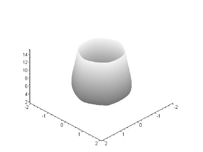
Figure 1: The shape of the relativistic potential in the equal mass case.

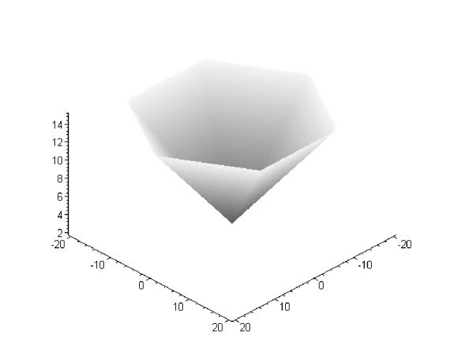
Figure 2: The shape of the non-relativistic potential in the equal mass case.

At very low energies these cases are indistinguishable. However striking differences between them develop quite rapidly with increasing energy, as figures 1 and 2 illustrate for the R and N systems. For all energies the Newtonian potential takes the form of the hexagonal-well potential noted earlier: equipotential lines form the shape of a regular hexagon in the $\left(\rho,\lambda\right)$ plane, with the sides rising linearly in all directions. The post-Newtonian potential retains this basic hexagonal symmetry, but distorts the sides to be parabolically concave. The growth of the potential is more rapid, with the sides of the potential growing quadratically with $\left(\rho,\lambda\right)$.

The exact potential differs substantively from both of these cases.  It retains the hexagonal symmetry, but the sides of the hexagon become convex, even at energies only slightly larger than the rest mass. The growth of the potential with increasing $V_{\textrm{R}}$ is extremely rapid compared to the other two cases, and so the overall size of the hexagon at a given value of $V_{\textrm{R}}$ is considerably smaller.  The size of the cross-sectional hexagon reaches a maximum at $V_{\textrm{R}}=V_{\textrm{R}c}=6.711968022mc^{2}$, after which it decreases in diameter like $\ln\left(V_{\textrm{R}}\right)/V_{\textrm{R}}$ with increasing $V_{\textrm{R}}$.

The part of the potential on the branch with $V_{\textrm{R}}>V_{\textrm{R}c}$ is in an intrinsically non-perturbative relativistic regime: the motion for values of $V_{\textrm{R}}$ larger than this cannot be understood as a perturbation from some classical limit of the motion. The non-relativistic hexagonal cone becomes a hexagonal carafe in the relativistic case, with a neck that narrows as $V_{\textrm{R}}$ increases.

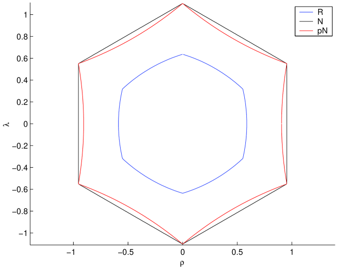
Figure 3: Equipotential lines at $V\simeq 4mc^{2}$ for each of the N, pN and R systems in the equal mass case.

Of course in both the pN and R systems the potential does not fully govern the motion since there are couplings between the momentum and position of the hex-particle.  In the post-Newtonian case we see that to leading order in $c^{-2}$ there is a momentum-dependent steepening of the walls of the hexagon.

For unequal masses the hexagon becomes squashed, with two opposite corners moving inward, changing both the slopes of the straight edges and their relative lengths; relativistic corrections maintain this basic distortion, but with the straight edges becoming parabolic. We shall not discuss the unequal mass case any further.

5 Methods for Solving the Equations of Motion

We begin our analysis of the $3$-body system by analyzing (studying) the motion of the hex-particle in the $\left(\rho,\lambda\right)$ plane. We shall consider this motion in the non-relativistic (N), post-Newtonian (pN) and exact relativistic (R) cases described in the previous section.  In all three cases the bisectors joining opposite vertices of the hexagon correspond to particle crossings in the full 3-particle system, and denote a discontinuous change in the hex-particle’s acceleration. Thus the hex-particle’s motion, in the Hamiltonian formalism, is described by a pair of differential equations that are continuous everywhere except across the three hexagonal bisectors $\rho=0$, $\rho-\sqrt{3}\lambda=0$, and $\rho+\sqrt{3}\lambda=0$. These bisectors divide the hexagon into sextants and correspond to the crossings of particles 1 and 2, 2 and 3, or 1 and 3 respectively.

An analogous system has been studied in the N system by Miller and Lehtihet, who considered the motions of a ball under a constant gravitational force elastically colliding with a wedge [13]. They established that such motions can be analyzed using a discrete mapping that describes the particle’s angular and radial velocities each time it collides with the edges of the wedge, which corresponds in our case to crossing one of the three hexagonal bisectors. The two systems differ in that in the wedge system the hex-particle collides elastically with the wedge (equivalent to an elastic collision between a pair of particles in the $3$-body system), whereas in our system the particle crosses the hexagon’s bisectors, equivalent to a pair of particles passing through each other in the $3$-particle system. In the equal mass case the systems are nearly identical, since an elastic collision between two equal mass particles cannot be distinguished from a crossing between two equal mass particles. We do, however, observe a distinction between the two systems in a certain class of orbits that we shall discuss later.

It is the non-smoothness of the potential along these bisectors that in all three cases yields interesting dynamics for the system. In our subsequent analysis we shall distinguish between two distinct types of motion [13]: $A$-motion, corresponding to the same pair of particles crossing twice in a row (the hex-particle crossing a single bisector twice in succession), and $B$-motion, in which one particle crosses each of its compatriots in succession (the hex-particle crossing two successive sextant boundaries). We can characterize a given motion by a sequence of letters $A$ and $B$ (called a symbol sequence), with a finite exponent $n$ denoting $n$-repeats and an overbar denoting an infinite repeated sequence. For example the expression $A^{4}B^{3}$ denotes four $A$-motions (two adjacent particles cross twice in a row four times in succession) followed by three $B$-motions (one particle crosses the other two in succession, which then cross each other). In the $\left(\rho,\lambda\right)$ plane this will correspond to a curve that  crosses (for example) the $\rho=0$ axis $4$ times before crossing one of the other sextant boundaries, after which it crosses two more sextant boundaries in succession, ending up in a sextant $180^{o}$ opposite to the one in which it began.  The expression $\left(A^{n}B^{m}\right)^{p}$ denotes $p$-repeats in succession of the motion $A^{n}B^{m}$, and $\overline{\left(A^{n}B^{m}\right)}$ denotes infinitely many repeats of this motion. Note that the classification of a crossing motion as $A$ or $B$ is contingent upon the previous crossing, and so there is an ambiguity in classification of either the final or the initial crossing.  We shall resolve this ambiguity by taking the initial crossing of any sequence of motions as being unlabeled – as we are considered arbitrarily large sequences of motions, this ambiguity in practice causes no difficulties.

We have carried out three methods of analysis to study the motions of this system. First, we plot trajectories of the hex-particle in the $\rho$- $\lambda$ plane, comparing the motions of the N, pN, and R systems for a variety of initial conditions. Second, we plot the motions of the three particles as a function of time for each case. This provides an alternate means of visualizing the difference between the various types of motion that can arise in the system. Third, we construct Poincare sections by recording the radial momentum ($p_{R}$, labelled as $x$) and the square of the angular momentum ($p_{\theta}^{2}$, labelled as $z$) of the hex-particle each time it crosses one of the bisectors. When all three particles have the same mass, all bisectors are equivalent, so that all the crossings may be plotted on the same surface of section.   This allows us to find regions of  periodicity, quasi-periodicity and chaos, and we shall discuss these features in turn.

One issue that arises upon comparison between the three systems is that the same initial conditions do not yield the same conserved energy.  There is therefore some ambiguity in comparing trajectories between each of these three cases: one can either compare at fixed values of the energy, modifying the initial conditions as appropriate (as required by the conservation laws for each system), or else fix the initial conditions, comparing trajectories at differing values of $H$.  We shall consider both methods of comparison. In the former case we fix the initial values of $H,\rho,\lambda$ and $p_{\rho}$, adjusting $p_{\lambda}$ so that the Hamiltonian constraint (55) is satisfied. We shall refer to these conditions as fixed-energy (FE) conditions. In the latter situation we set the initial values of all four phase-space coordinates $\left(\rho,\lambda,p_{\rho},p_{\lambda}\right)$ in each system, allowing the energy to differ for each of the N, pN, and R systems according to the respective constraints (74), (73) and (55) for each. We shall refer to these conditions as the fixed-momenta (FM) conditions.

There is no closed-form solution to either the determining equation (55) or to the equations of motion (59,60), and so to analyze the motion we must solve these equations numerically. We did this by numerically integrating the equations of motion using a Matlab ODE routine (ode45, or for the exact solutions, ode113). To generate Poincare sections, we stopped the integration each time the hex-particle crossed one of the bisectors by using an ‘events’ function, saving the values of the radial and angular momentum for plotting. Ideally, for each chaotic trajectory the Poincare section should be allowed to run for a very long time in order to determine as accurately as possible which regions of the plane it may visit, and which are off-limits.

As a control over errors, we imposed absolute and relative error tolerances of $10^{-8}$ for the numerical ODE solvers. For the values of $\eta$ we studied, this yielded numerically stable solutions. We tested this by checking that the energy remained a constant of the motion for all three systems to within a value no larger than $10^{-6}$; for nearly all of our runs it was comparable to the error tolerances ($10^{-8}$ ) that we imposed.

However we found that for $\eta\succapprox 1$ that the ODE solver was unable to carry out the integration for more than a few time steps for the R system before exceeding the allowed error tolerances (this problem remains even if the error tolerances are lowered significantly). This value of $\eta$ is approximately the value $V_{\textrm{R}c}$ at which the equipotential hexagon reaches its maximal size. We were unable to find an algorithm capable of handling the numerical instabilities, which the ODE solvers we employed could not deal with, for these larger values of $\eta$.  A full numerical solution in this larger $\eta$ regime remains an open problem.

We also found that the pN system had diverging trajectories for values of $\eta$ larger than $0.3$. We believe that this is due to an intrinsic instability in the pN system, but we have not confirmed this.

In addition to plots, a few other routines were used to record information. While running Poincare sections, the name of the edge crossed at each collision (corresponding to the pair of particles that pass through each other along that edge) can be recorded in addition to the velocity. From this information, the symbol sequence of the trajectory can be extracted. In addition, we recorded a frequency of return: this function measures the time interval separating the hex-particle’s successive returns to within some small distance of its original location, and takes its inverse to find a ‘frequency’ at each time. The value of frequency depends strongly on how small the specified area is; nonetheless, these ‘frequencies’ give us an approximate idea of how long the hex-particle takes to complete one full cycle in its ‘orbit’.

In performing our numerical analysis we rescale the variables

$$p_{i}=M_{tot}c\hat{p_{i}}\textrm{ \ \ \ \ \ \ \ \ \ \ }z_{i}=\frac{4}{\kappa M_{tot}c^{2}}\hat{z_{i}}$$ (78)

where $M_{tot}=3m$ is the total mass of the system and $\hat{p}_{i}$ and $\hat{z}_{i}$ are the dimensionless momenta and positions respectively. Writing $\eta+1=H/M_{tot}c^{2}$, $\hat{m_{i}}=(\frac{m_{i}}{M_{tot}})$,  we have

$$M_{i} = M_{tot}c^{2}\left(\sqrt{\hat{p_{i}}^{2}+\hat{m_{i}}^{2}}+\hat{p_{i}}\right)=M_{tot}c^{2}\hat{M}_{i}$$ (79)

$$L_{i} = M_{tot}c^{2}\left(\eta+1-\sqrt{\hat{p_{i}}^{2}+\hat{m_{i}}^{2}}-\epsilon(\sum_{j}\hat{p}_{j}s_{ji})\right)\textrm{\ \ }=M_{tot}c^{2}\hat{L}_{i}\textrm{\ \ \ \ }$$ (80)

which in turn yields

$$\hat{L}_{1}\hat{L}_{2}\hat{L}_{3} = {\mathfrak{\hat{}}{M}}_{12}{\mathfrak{\hat{}}{M}}_{21}\hat{L}_{3}^{\ast}e^{s_{12}[(\hat{L}_{1}+{\mathfrak{\hat{}}{M}}_{12})\hat{z}_{13}-(\hat{L}_{2}+{\mathfrak{\hat{}}{M}}_{21})\hat{z}_{23}]}$$ (81)

$$+{\mathfrak{\hat{}}{M}}_{23}{\mathfrak{\hat{}}{M}}_{32}\hat{L}_{1}^{\ast}e^{s_{23}[(\hat{L}_{2}+{\mathfrak{\hat{}}{M}}_{23})\hat{z}_{21}-(\hat{L}_{3}+{\mathfrak{\hat{}}{M}}_{32})\hat{z}_{31}]}$$

$$+{\mathfrak{\hat{}}{M}}_{31}{\mathfrak{\hat{}}{M}}_{13}\hat{L}_{2}^{\ast}e^{s_{31}[(\hat{L}_{3}+{\mathfrak{\hat{}}{M}}_{31})\hat{z}_{32}-(\hat{L}_{1}+{\mathfrak{\hat{}}{M}}_{13})\hat{z}_{12}]}$$

for the rescaled determining equation. Similarly the equations of motion become

$$\frac{\partial\eta}{\partial\hat{p_{i}}} = \frac{1}{c}\frac{\partial H}{\partial p_{i}}=\frac{4}{\kappa M_{tot}c^{3}}\frac{d\hat{z}_{i}}{dt}=\frac{d\hat{z}_{i}}{d\hat{t}}$$ (82)

$$\frac{\partial\eta}{\partial\hat{z_{i}}} = (\frac{4}{\kappa M_{tot}^{2}c^{4}})\frac{\partial H}{\partial z_{i}}=-\frac{4}{\kappa M_{tot}c^{3}}\frac{d\hat{p_{i}}}{dt}=-\frac{d\hat{p_{i}}}{d\hat{t}}$$ (83)

where $t=\frac{4}{\kappa M_{tot}c^{3}}\hat{t}$.  A time step in the numerical code has a value $\hat{t}=1$.  All diagrams will be shown using the rescaled coordinates (78) unless otherwise stated.

We close this section with some final comments regarding the time variable $t$. This parameter is a coordinate time and it would be desirable to describe the trajectories of the particles in terms of some invariant parameter. The natural candidate is the proper time $\tau_{a}$ of each particle. From equations (18), the proper time is

$$d\tau_{a}^{2} = dt^{2}\left\{N_{0}(z_{a})^{2}-(N_{1}(z_{a})+\dot{z}_{a})^{2}\right\}\;,$$ (84)

$$= dt^{2}N_{0}(z_{a})^{2}\frac{m_{a}^{2}}{p_{a}^{2}+m_{a}^{2}}\qquad\qquad(a=1,2,3)\;\;.$$

for the $a$th particle.  Unfortunately this is in general different for each particle, even in the equal mass case. This is quite unlike the two-body situation, in which the symmetry of the system yields the same proper time for each particle in the equal mass case (though not for the unequal mass case) [7].

There are several different choices available at this stage. One could choose to work with the proper time of a single particle in the system, in which case invariance is recovered, but the manifest permutation symmetry between particles is lost. Another possibility is to construct a ‘fictitious’ fourth particle that does not couple to the other three, but moves along a geodesic of the system, and make use of its proper time.  Rather than consider these or other possible options, we shall postpone their consideration for future research and work with $t$, keeping in mind that it is a coordinate time.

6 Equal Mass Trajectories

The three systems (N, pN, R) we consider here constitute a family of related systems whose dynamics one would expect to be similar (but not identical) at small energies, with increasingly different behaviour emerging as the energy increases. However, our examination of the symbolic sequence of various equal mass trajectories reveals a strong set of similarities, in that certain types of sequences are common to all three systems over the energy range we considered. We find that the types of motion exhibited by this family of systems may thus be divided into three principal classes, which we denote by the names annuli, pretzel and chaotic.

Before discussing each of these classes in detail, we make a few general remarks. First, within each class a further distinction must be made between those orbits which eventually densely cover the portion of $\left(\rho,\lambda\right)$ space they occupy, and those which do not. (By definition, all of the chaotic orbits densely cover their allowed portion of phase space). The latter situation corresponds to regular orbits in which the symbol sequence consists of a finite sequence repeated infinitely many times. The former situation corresponds to orbits that are quasi-regular: the symbol sequence consists of repeats of the same finite sequence, but with an $A$-motion added or removed at irregular intervals.

These two types of orbits are separated in phase space by separatrixes (trajectories joining a pair of hyperbolic fixed points). Regular orbits lie inside the ‘elliptical’ region surrounding an elliptical fixed point; the quasi-regular orbits lie outside such a region.

It is useful to further distinguish between the quasi-periodic and periodic regular orbits. Quasi-periodic trajectories closely resemble the related periodic trajectories, except that the orbit fails to exactly repeat itself and hence eventually densely covers some region of phase space. Thus a quasi-periodic trajectory displays a high degree of regularity. In the system we study, this regularity is manifest by its periodic symbol sequence. The classic example of this is a particle moving on a torus $S^{1}\times S^{1}$. The motion is characterized by its angular velocity around each copy of $S^{1}$: if the ratio of these is rational, the motion will be periodic; if it is irrational, the motion will be quasi-periodic. For the system considered here, non-periodic orbits with fixed symbol sequences are quasi-periodic. They appear as a collection of closed circles, ovals, or crescents in the Poincare section. Orbits with symbol sequences that are not fixed, however, are distinctly not regular; we shall refer to them as quasi-regular as noted above.

We also note that, although the orbits of the non-relativistic and relativistic systems realize the same symbol sequences, important qualitative differences exist between these orbits for both the trajectories and the Poincare sections. Consider a comparison between each system at identical values of the total energy $H=E_{T}$ and the initial values of $\left(\rho,\lambda,p_{\rho}\right)$, with the remaining initial value of $p_{\lambda}$ chosen to satisfy (55,73,74) in each respective case.  As $\eta=H/\left(3mc^{2}\right)-1$ increases, distinctions between the exact relativistic and non-relativistic cases become substantive, both qualitatively and quantitatively. The relativistic trajectories have higher frequencies and extend over a smaller region of the $\left(\rho,\lambda\right)$ plane than their non-relativistic counterparts.  Their trajectory patterns in the pretzel class also develop a slight “hourglass” shape (narrowing with increasing $\eta$ in the small-$\lambda$ region) in comparison to the cylindrical shapes of their non-relativistic counterparts.

At FM initial conditions, we find in general that the R system has greater energy than its corresponding N and pN counterparts. Hence in these cases we find that the R orbits cover a correspondingly larger region of the $\left(\rho,\lambda\right)$ plane and have a higher frequency.

6.1 Annulus Orbits

The annuli are orbits in which the hex-particle never re-crosses the same bisector twice. All such orbits have the symbol sequence $\overline{B}$, and describe an annulus encircling the origin in the $\rho-\lambda$ plane.

As noted above, we see that some annulus orbits are quasi-periodic and fill in the entire ring (generating one of the closed triangle-like shapes in the middle of the Poincare section) while a choice few apparently repeat themselves after some number of rotations about the origin. This latter situation is illustrated in figs. 4, 5 and 6 for the N, pN and R cases respectively.  In each of these cases a wide variety of patterns emerge contingent upon the initial conditions but independent of the system in question. Both these orbits and those that fill in the ring (not illustrated) are ‘close to’ an elliptic fixed point; the difference between them is that in some cases the normally quasi-periodic orbits have commensurate winding numbers, producing an eventually periodic orbit. As periodic orbits are difficult to find numerically, the orbits in the figures are actually orbits that are very close to periodic orbits, so that the pattern of the periodic orbit is still visible. In fact they are quasi-periodic orbits about these higher-period fixed points, which means that they will not cover the entire annulus, only bands of phase space.

We find no qualitative distinctions between the N and pN annuli up to the values of $\eta$ that we can attain numerically. However we do find that the R cases appear to undergo a slight rotation relative to their N counterparts as $\eta$ increases. This is noticeable in the right-hand diagrams of fig.6, for $\eta=0.75$ and $\eta=0.9$.

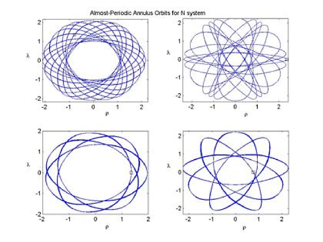
Figure 4: Examples of almost-periodic annuli for the N system: trajectories do not cover the entire annulus band (run for 200 time units).  A wide variety of complex patterns can be found. The square indicates the intial values of $\left(\rho,\lambda\right)$; FM initial conditions were employed.

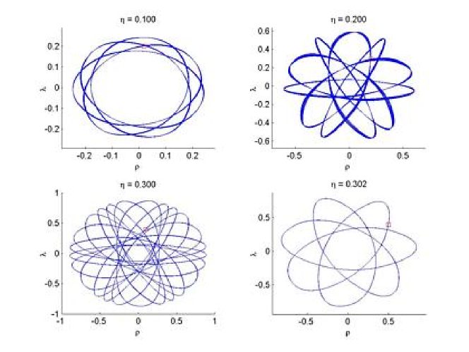
Figure 5: Examples of almost-periodic annuli for the pN case (trajectories run for 200 time units).  Up to the values of $\eta$ attainable numerically, no differences were observed between PN and N annulus-type orbits. The square indicates the intial values of $\left(\rho,\lambda\right)$; FM initial conditions were employed.

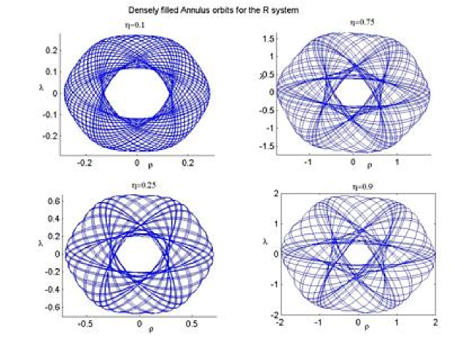
Figure 6: A sampling of densely-filled annuli for the R solution. All orbits were run for 200 time steps using FE initial conditions. Densely filled annuli can be found for all values of $\eta$.  As $\eta$ increases, the R annuli rotate with increasing angle relative to their N counterparts; the orientation (clockwise or anticlockwise) depends upon the initial conditions.

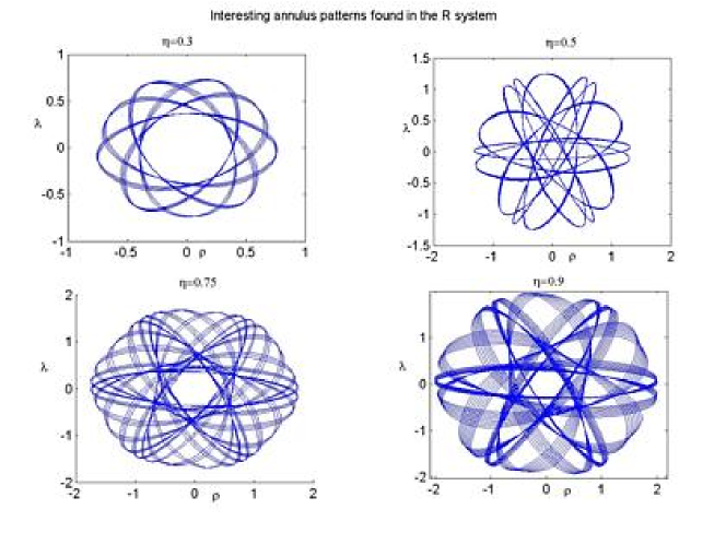
Figure 7: A sampling of quasi-periodic annuli for the R system, run for 200 time steps and FE initial conditions.  As in the N and pN systems, various periodic, quasi-periodic, and densely filled annuli can be found for all $\eta$.  

In figures 8,9 we plot the positions of each of the three bodies as a function of time in conjunction with their corresponding trajectories in the $\left(\rho,\lambda\right)$ plane for FE conditions in both the N and R cases.    We see that at similar energies a $3$-body system experiencing relativistic gravitation covers the $\left(\rho,\lambda\right)$ plane in the hex-particle representation more densely than its non-relativistic counterpart, and induces a higher frequency of oscillation. This higher frequency is also characteristic of the $2$-body system [5, 8], and we have observed it to be a general phenomenon for all FE conditions we have studied.  The increased trajectory density for FE conditions is also a phenomenon we observe to generally occur for the $3$-body R system, presumably because both systems were run for the same number of time steps, and the relativistic one has a higher frequency.

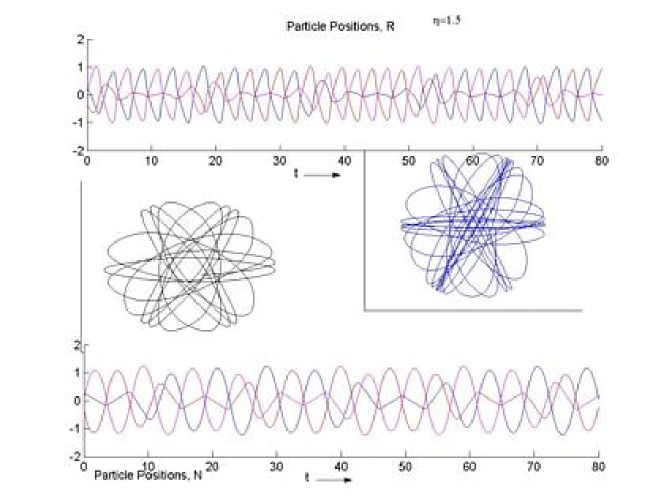
Figure 8: Near-chaotic annulus orbits (N-black, R-blue) shown in conjunction with their corresponding 3-particle trajectories. These near-chaotic orbits have been run for 200 time steps using FE initial conditions. We have truncated the 3-particle trajectory plot after 80 time steps. The R trajectory is closer to chaos than the N trajectory.

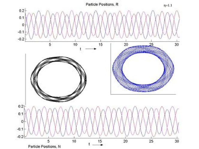
Figure 9: Annulus orbits (N-black, R-blue) shown in conjunction with their corresponding 3-particle trajectories. These quasi-regular orbits have been run for 200 time steps using FE initial conditions and are far from being chaotic. We have truncated the 3-particle trajectory plot after 30 time steps.  The R motion is further from periodicity, leaving far fewer open regions in the $\left(\rho,\lambda\right)$ plane.

A comparison of orbits using FM initial conditions is also instructive; fig. 10 provides an example. At FM conditions the R system typically has slightly higher energy, and so covers a considerably larger region of the $\left(\rho,\lambda\right)$ plane more densely than its non-relativistic counterpart, venturing slightly closer to the origin. This effect increases with increasing $\eta$, provided that the R energy remains larger than its N counterpart.  However as $\eta$ gets larger it becomes increasingly more difficult to find initial conditions such that both the N and R annuli are close to periodic orbits.  The bottom diagram in fig. 10 is an example at $\eta\simeq 0.5$; the N system has about 14% more energy than its R counterpart, and so it now covers a larger region.

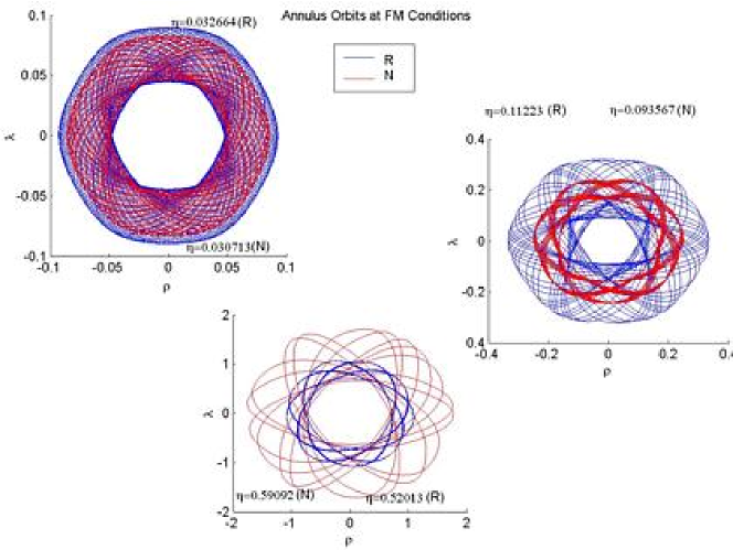
Figure 10: A comparsion of annulus orbits at identical FM conditions, for three similar values of $\eta$.  With identical initial conditions, the relativistic trajectories typically have greater energy and so cover a larger region of the $\left(\rho,\lambda\right)$ plane. However for some initial conditions the N system has a larger energy and so covers a correspondingly larger region. All orbits were run for 200 time steps.

Figure 11 illustrates the temporal development of an annulus pattern for $\eta=0.9$ in the R system. At all values of $\eta$ investigated, annuli evolution is qualitatively the same in the N, pN and R systems, although the shape of the annulus itself changes.

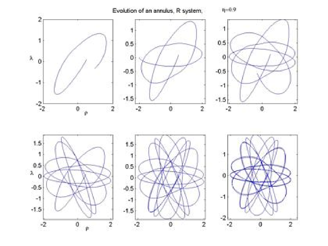
Figure 11: Early time development of a densely filled annulus in the R system with $\eta=0.9$, shown at $t=5,12,20,30,45$ and $60$ time steps. The evolution of annuli is qualitatively the same in the N, pN and R systems at all values of $\eta$ investigated, although the orientation and scale of the anulus itself changes in the R case.  

6.2 Pretzel Orbits

Pretzel orbits are those in which the hex-particle essentially oscillates back and forth about one of the three bisectors, corresponding to a stable or quasi-stable bound subsystem of two particles. Symbolically such orbits can be written as $\prod_{ijk}\left(A^{n_{i}}B^{3m_{j}}\right)^{l_{k}}$ , where $n_{i},m_{j},l_{k}\in Z^{+}$, with some $l_{k}$ possibly infinite. The resulting collection of trajectories is extremely diverse. Many families of regular orbits exist. Such families contain one base element (for example $AB^{3}$) and a sequence of elements formed by appending an $A$ to each existing sequence of $A$’s (for example, $\{AB^{3},A^{2}B^{3},A^{3}B^{3},...\}$. The result is that the phase space has an extremely complex structure that we shall discuss further in section 7. It is differences in this structure and the shapes of the corresponding orbits that show the most remarkable distinctions between the R, PN and N systems.

In the above sequences, the $B^{3}$ sequence corresponds to a 180-degree swing of the hex-particle around the origin, and the resultant figures in the $\left(\rho,\lambda\right)$ plane comprise a broad variety of twisted, pretzel-like figures, from whence their name. This situation is a key distinction between the systems we study and the wedge system [13] discussed earlier. In the wedge system $B$ and $B^{2}$ sequences are observed in addition to $B^{3}$ sequences; we observe only the latter in all pretzel orbits.

Before proceeding to a detailed description of this class, we summarize the main results of our investigation. Again we have both regular orbits (with the symbol sequence above repeating ad infinitum) and non-regular orbits that densely fill a cylindrical tube in the $\left(\rho,\lambda\right)$ plane. The periodic and quasi-periodic orbits we find in the N system appear for the most part to have counterparts with the same symbol sequence in the R system (though not in the pN system). In general orbits in the R system have kinks about the $\lambda=0$ line relative to their N and pN counterparts; for example a cylindrical-shaped trajectory in the N system looks like an hourglass in the R system.  The pN system exhibits chaotic behaviour not seen in the N and R systems, a point we shall discuss in a subsequent section.

Figures 12 and 13 illustrate the development of a trajectory in the $\left(\rho,\lambda\right)$ plane for FE conditions at small and large values of $\eta$. As expected we see that for small $\eta$ ($\eta=0.05$) there is very little distinction between the N and R motions, consistent with the smooth non-relativistic limit of (55).  However at larger $\eta$ ($\eta=0.85$) the hex-particle traces out significantly different trajectories in the N and R systems. The oscillation frequency is higher and the trajectory is more tightly confined, features commensurate with $2$-body motion in the R system [5, 8, 6].  We also see a considerably different weave pattern in fig 13 for each case, with the N pattern exhibiting a near-cylindrical shape in contrast to its R counterpart with oscillating sides.

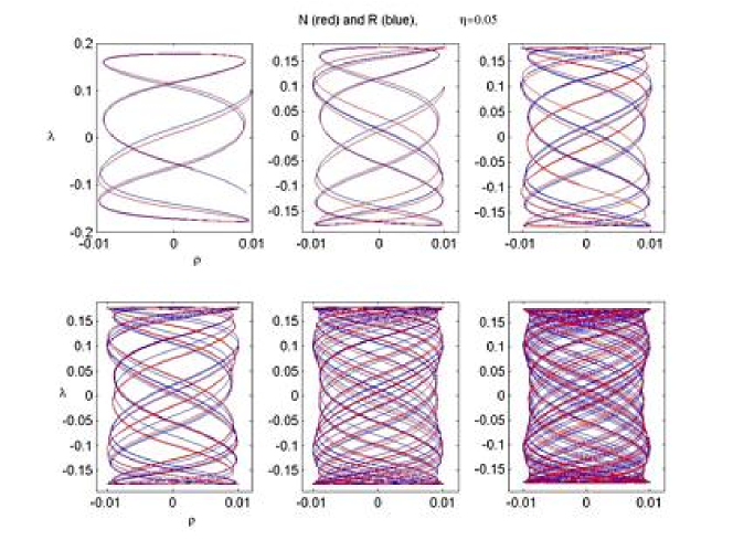
Figure 12: A time series evolution for a pretzel orbit shown simultaneously in the N and R systems at t=3,6,11,16,25,and 35 units for $\eta=0.05$ at FE conditions.  The trajectories in the two systems are very similar at such low energies.  

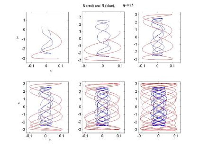
Figure 13: N and R pretzel orbits evolving simultaneously at t=3,6,11,16, 26, and 36 units for $\eta=0.85$ with FE conditions. The N trajectory extends considerably further from the origin, while the R orbit evolves with a higher collision frequency. The R orbit has stabilized into a quasi-periodic pattern, whereas the N orbit will eventually form a densely filled cylinder.

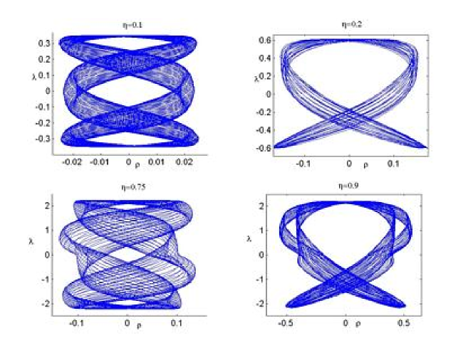
Figure 14: A comparison of similar quasi-regular pretzel-type orbits for the R case at different values of $\eta$.  The symbol sequence is $\overline{\left(A^{2}B^{3}\right)}$ for the trajectories on the left, and $\overline{\left(AB^{6}\right)}$ for the trajectories on the right. As $\eta$ increases the asymmetry due to relativity becomes increasingly apparent.  (Note that as $\eta$ changes, the initial conditions required to find a given orbit also alter.)

In fig. 15 we compare the positions of each of the three bodies as a function of time in conjunction with their corresponding trajectories in the $\left(\rho,\lambda\right)$ plane for two slightly different FE conditions in the R system. The fish-like diagram corresponds to an $AB^{6}$ symbol sequence: we see that two of the particles oscillate quasi-regularly about each other, this pair undergoing larger-amplitude and lower-frequency oscillations with the third.  A slight change of initial conditions yields the strudel-like figure; here we see that one particle alternates its oscillations with the other two, maintaining a near-constant amplitude throughout.

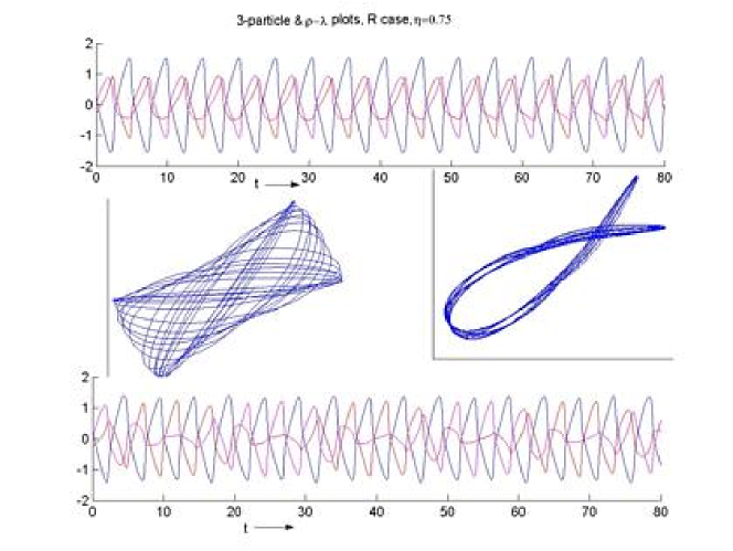
Figure 15: Pretzel orbits of the relativistic system with the corresponding $3$-particle time evolution: a regular $AB^{6}$ orbit pattern (top), and similar irregular orbit pattern, at slightly different initial conditions (bottom). Both cases employ FE conditions, and were run for 200 time steps, with the $3$-particle trajectory plot truncated after 80 time steps.

We compare in figure 16 pretzel orbits with the same FE conditions in the R and N cases plotted as trajectories in the $3$-body system. These orbits are distinguished by having a very high-frequency low-amplitude oscillation between two of the particles; this pair in turn undergoes a low-frequency high-amplitude oscillation with the third.  The red and blue lines are nearly indistinguishable due to their close proximity; the inset in the figure provides a close-up of the oscillations in this two-body subsystem near one of its extrema. The N oscillations are parabolic in shape whereas the R oscillations have the shoulder-like distortion seen previously in the $2$-body system [5]. These diagrams illustrate that under appropriate initial conditions two bodies can tightly and stably bind together in both the N and R systems (even at substantively large $\eta$), behaving like a single body relative to the third.

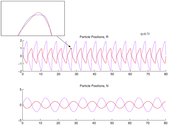
Figure 16: A pretzel-orbit with a large number of $A$ collisions before the $B^{3}$ collision sequence, run with FE intial conditions.  Particles 1 and 2 (red and blue lines respectively) remain very close together, colliding frequently.  They act much like a single body from the viewpoint of particle 3; the above trajectory bears a strong resemblance to the trajectories found in the 2-body case. The inset shows detail near the one of the peaks in the R system.

A similar situation is shown in fig. 17, where FE initial conditions were employed. The oscillations for the $2$-body subsystem are now of lower frequency and larger amplitude than in fig. 15, and the symbol sequences differ between the N and R cases. The respective parabolic regularity and shoulder-like distortions are evident, and the $2$-body subsystem oscillations in the R case are of slightly larger amplitude and higher frequency than in its N counterpart.

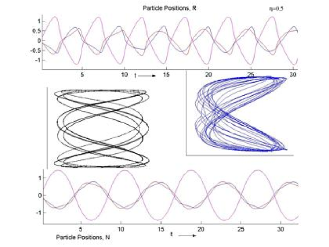
Figure 17: Regular pretzel orbits (run for 120 time steps) of the R and N systems with the corresponding $3$-particle time evolution (truncated at 35 time steps). These orbits correspond to the collision sequences $AB^{3}$ (R) and $A^{2}B^{3}$ (N).  Since we employ FE initial conditions the collision sequences differ.

We can obtain interesting sequences of orbits of the hex-particle by controlling the FM initial conditions. Consider for example fig. 18, which consists of members of a family of quasi-regular orbits given by $\left\{\overline{A^{i}B^{3}}\right\}$ for the N case.  These snake-like orbits have two sharp turning points separated by some number $n\$ of bumps, and correspond to sequences of $2(n+2)$ circles in the lower portion of the Poincare section. Such orbits have been shown to exist for arbitrary $n$ in the N system [13].  We have found such orbits up to $n=15$ and conjecture that they also exist for arbitrary $n$ in the R and pN systems below the threshold of chaos. In the pN system, orbits of higher $n$ are gradually destroyed by chaos as $\eta$ increases, with more and more of the pretzel region becoming chaotic. We have found some evidence (see the next section) that this may also occur in the R system; if so, the onset of chaos will be much less dramatic than in the pN case. The corresponding situation for the R system is shown in fig. 19, with $\eta=0.75$.  The collision sequences are the same, as is their correspondence with the circles in the lower portion of the Poincare section. However the figures in the R system develop an hourglass shape, narrowing about $\lambda=0$, whereas the N orbits are circumscribed by a cylinder.

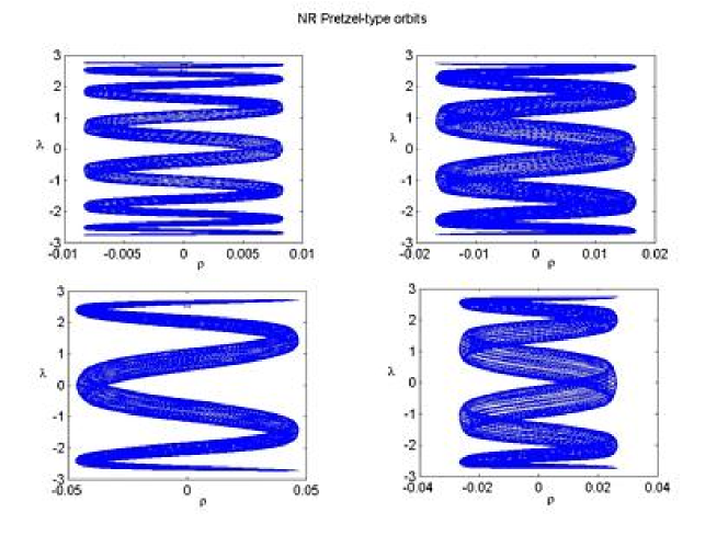
Figure 18: A family of quasi-regular snake-like orbits for the N system, each with two sharp turning points separated by some number $n$ of bumps. All were run for 200 time steps with FM initial conditions; the square indicates the starting point in the $\left(\rho,\lambda\right)$ plane. These orbits have the symbol sequence $A^{m}B^{3}$ for $m$ odd, and correspond to sequences of even numbers ($2(n+2)$) of circles in the lower portion of the Poincare section.  The value of $n$ increases with decreasing initial angular momentum. It appears that such orbits exist for arbitrary $n$; we have found them up to $n=15$.

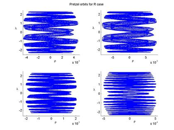
Figure 19: Orbits from the same family for the R system with $\eta=0.75$. (Here FE initial conditions were used, so only qualitative features may be compared.)  The N and R orbits in this family have collision sequences of the form $A^{m}B^{3}$ ( $m$ odd); however, the R orbits have an hourglass shape, while the N orbits in fig. 18 lie in a cylinder.  

In fig. 20 we compare orbits with the symbol sequence $AB^{3}$.  Here we see another example of how relativistic effects induce qualitatively different features not seen in the N system.  As $\eta$ increases, orbits in the R system develop two distinct turning points at different distances from the $\rho=0$ axis. This is particularly evident for $\eta=0.75$. There is also the development of a kink at the right-hand-side of the Boomerang figure that becomes increasingly more pronounced with increasing $\eta$. The underlying reason behind the development of this structure is not clear to us; however we do not see it in the N system.

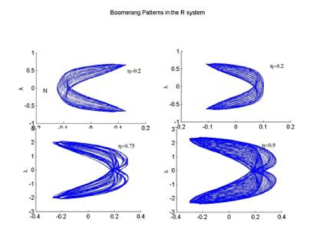
Figure 20: An orbit with the symbol sequence $AB^{3}$, shown for the N system (plot 1), and the R system at different $\eta$ values (plots 2-4).  All figures were run for 200 time steps with FM initial conditions.  Note that as $\eta$ increases, the R trajectories develop a kink along the $\lambda=0$ axis, and begin to display a double-banding pattern with two turning points at two distinct distances from the $\rho$ axis about $\lambda=0$.

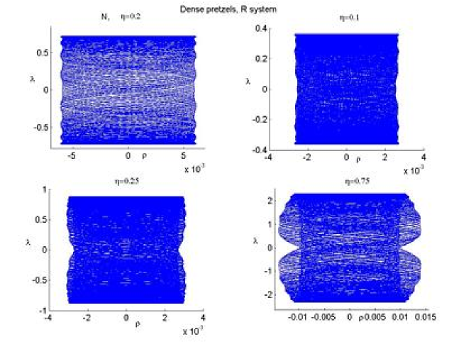
Figure 21: Densely filled orbits in the pretzel class for the R system at varying values of $\eta$, run for 200 steps with FE initial conditions. A diagram for the N system at $\eta=0.2$ is included in the upper left for comparative purposes. As $\eta$ increases, the R orbits take on an increasingly pronounced hourglass shape.  In the R system, we do not observe the breakdown to chaos seen in the pN case (fig.23 ).

Overall the variety of orbits that appear in the R system appears to have a richer and more detailed structure than that of the N system; for example there are indentations in the bowtie patterns, the cylindrical shapes in the N system become hourglass shapes in the R system and so on. Fig. 22  illustrates this for $\eta=0.9$; we see variants of the hourglass effect in two of these figures, along with different manifestations of the development of distinct turning points.

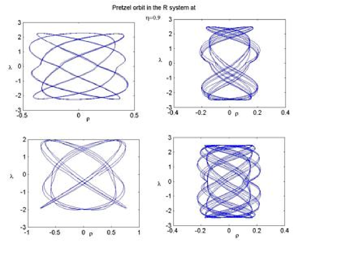
Figure 22: A survey of the broad variety of figures in the R system that arise in the pretzel class for $\eta=0.9$.   All orbits were run for 200 time steps with FE initial conditions.

6.3 Chaotic Orbits

The chaotic orbits are those in which the hex-particle wanders between $A$-motions and $B$-motions in an apparently irregular fashion. Such orbits eventually wander into all areas of the $\rho-\lambda$ plane– a trait neither the annuli nor the pretzels possess. The major area of chaos found in all 3 systems occurs at the transition between annulus and pretzel orbits, where the hex-particle passes very close to the origin.

The most striking feature of this class of motions is the distinction between the pN system and its N and R counterparts.  We find that the pN system possesses an additional area of chaos in the pretzel region, a phenomenon we shall discuss in more detail in the next section.

We can observe the transition to chaos in the pretzel region of the pN system by slowly adjusting the value of $\eta$ for FE initial conditions. Figure 23 illustrates an example.  We begin with a pretzel diagram at $\eta=0.1$. As $\eta$ increases, the trajectory changes shape but remains regular until $\eta\simeq 0.22$ where the diagram appears slightly less ordered. At $\eta\simeq 0.28$ the hex-particle begins to irregularly traverse increasingly larger regions of the $\left(\rho,\lambda\right)$ plane, signifying the onset of chaos.

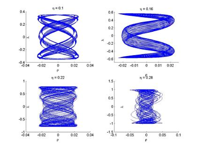
Figure 23: Transition to chaos for pretzel-type orbits in the pN case. All four trajectories were run for 200 time steps with the same FE initial conditions (with varying $\eta$). As $\eta$ increases, we see the densely filled pretzel regions become less ordered. At $\eta=0.28$ (lower right plot) we see the onset of chaos signified by an erratic trajectory exploring a much larger area in the $\rho$-$\lambda$ plane.

We plot in fig. 24 the transition in the R system with $\eta=0.5$ from an annulus to a pretzel orbit.  The transition, which goes from left-to-right and top-to-bottom with decreasing initial angular momentum, passes through a chaotic set of orbits. The chaotic trajectories pass very close to or through the origin, a characteristic feature for this region of chaos in all three systems.

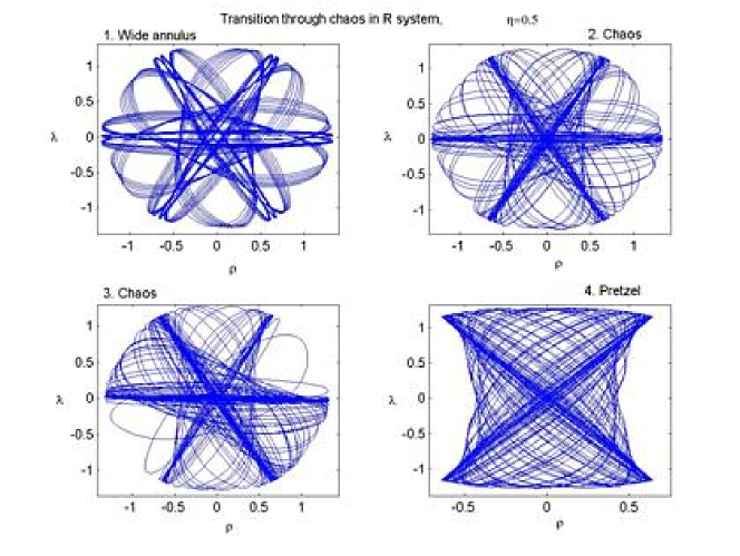
Figure 24: Transition from an annulus to a pretzel orbit through a chaotic region in the R system for $\eta=0.5$ as initial angular momentum in the $\left(\rho,\lambda\right)$ plane decreases. All diagrams were run for 450 time steps with FE initial conditions. Note that the chaotic trajectories pass very close to or through the origin.

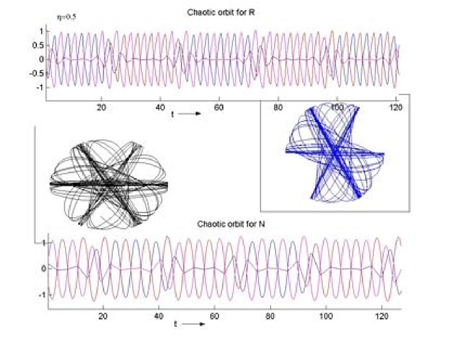
Figure 25: Chaotic orbits in the region of phase space separating annulus and pretzel trajectories.  Shown here are trajectories for R and N systems in the $\left(\rho,\lambda\right)$ plane (run for 300 time steps) and for the 3-body system (truncated at 120 time steps).  FE initial conditions were employed, but the initial values of $\left(\rho,\lambda,p_{\rho}\right)$ differ for the R and N trajectories shown. In the 3-body system, the particles spend most of their time in a configuration where one middle (‘m’) particle remains essentially motionless.  The motion appears very close to regular, its erraticity apparent in slight irregularities between the number of crossings for which one particle remains almost stationary. This causes the m-particle to alternate in an irregular fashion.

Figures 26 and 27 illustrate the time-development of a corresponding pair of chaotic trajectories in the R and N systems for different initial conditions. We see that different initial conditions at the same energy can yield a chaotic R trajectory whose N counterpart is an annulus, as well as a chaotic N trajectory whose R counterpart is a cylinder in the pretzel class.  In both cases we see that the R trajectory approaches its final pattern much more rapidly than its N counterpart (again, probably due to the difference in frequencies), regardless of whether or not the final state is chaotic.

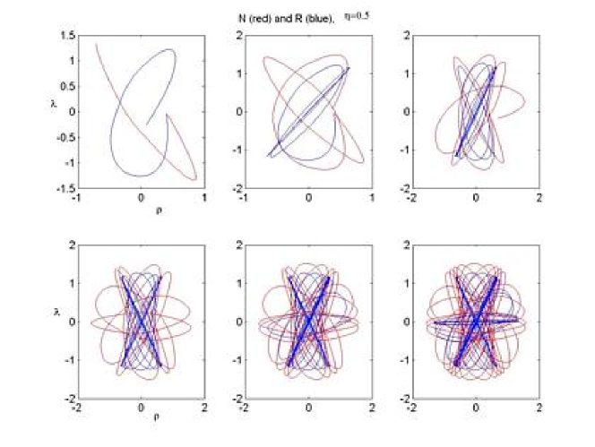
Figure 26: A comparison of the time-development of a chaotic R trajectory at $\eta=0.5$ with its N counterpart at the same energy (FE intial conditions), shown at $t=5,15,30,50,80$ and $110$ units. The N trajectory forms a densely filled annulus whilst its R counterpart is chaotic.

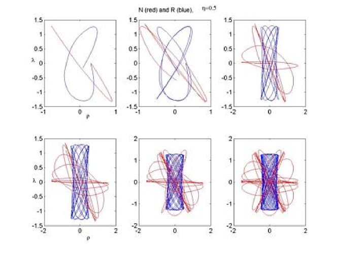
Figure 27: A comparison of the time-development of a chaotic N trajectory at $\eta=0.5$ with its R counterpart at the same energy (FE intial conditions), shown at $t=5,15,30,50,80$ and $110$ units. The R trajectory forms a densely filled cylinder in the pretzel class whilst its N counterpart is chaotic.

In all three systems there is a region of chaos (R1) between the pretzel and annulus type orbits, though in the R system it appears to shrink as $\eta$ increases. Secondly, in the pN system, chaotic pretzel orbits are also observed, becoming wilder and more prevalent with increasing $\eta$. These chaotic pretzel orbits, unlike their R counterparts, do not cover the entire $\left(\rho,\lambda\right)$ plane, as can be seen from the figure 23.

7 Poincare plots

We turn now to consider the Poincare sections for the three systems N, pN, R. These are constructed by plotting the square of the angular momentum ($p_{\theta}^{2}$, labelled as $z$) of the hex-particle against its radial momentum ($p_{R}$, labelled as $x$) each time it crosses one of the bisectors. Our conventions for these quantities are the same as in ref.[13], apart from an overall normalization for each section that we plot. All bisectors are equivalent since all three particles have the same mass, and we can plot all crossings on the same surface of section, allowing us to find regions of periodicity, quasi-periodicity and chaos.

Each of these systems is governed by a time-independent  Hamiltonian with four degrees of freedom. Hence the total energy is a constant of the motion, and the phase space for each system is a 3-dimensional hypersurface in 4 dimensions. If an additional constant of the motion exists, the system is said to be integrable, and its trajectories are restricted to two-dimensional surfaces in the available phase space. Since trajectories may never intersect, such a constraint imposes severe limitations on the types of motion that integrable systems can exhibit: trajectories may be periodic, repeating themselves after a finite interval of time, or quasi-periodic. The trajectories of an integrable system always appear as lines or dots, for periodic (1-dimensional) orbits on the Poincare section, as they comprise by definition the intersection of two 2-dimensional surfaces. This contrasts sharply with the case when a system is completely non-integrable, so that all orbits move freely in three dimensions. The extra degree of freedom permits orbits to visit all regions of phase space, and the system typically displays strongly chaotic behavior. Such trajectories appear as filled in areas on the Poincare map.

When an integrable system is given a sufficiently small perturbation, most of its orbits remain confined to two-dimensional surfaces . However small areas of chaos appear, sandwiched between the remaining two-dimensional surfaces. As the magnitude of the perturbation is increased, the chaotic regions grow, and eventually become connected areas on the Poincare section. This phenomenon is called a Kolmogorov, Arnold and Moser (KAM) transition [22]. Islands of regularity may remain for quite some time, and generally have an intricate fractal structure. For sufficiently large perturbations, however, systems typically become almost fully ergodic [23].

The structure of the Poincare section in the N system has already been studied to a certain extent in the wedge problem. In the equal mass case 3-body motion in the N system corresponds to motion of a body falling toward a wedge whose sides are each at angles $30^{o}$ relative to the vertical axis [13].   The outer boundary of the plot is determined by the energy conservation relation (74), which is

$$x^{2}\leq 1-z$$ (85)

where the energy $H-3mc^{2}$ has been normalized to unity (more generally, $x^{2}\leq\frac{2}{3}\eta-z$ for the unconstrained normalizations we employ). Equality in (85) holds when the hex-particle is at the origin, and yields the phase-space limit since any departure from the origin will reduce the values of $\left(x,z\right)$ relative to this bound.   Another relevant boundary is that given by

$$\left(x-2\sqrt{3z}\right)^{2}\leq 1-z$$ (86)

which is the energy constraint after an $A$-collision has taken place. Equality corresponds to the point at which all three particles are coincident (the hex-particle is at the origin).  All points in phase space satisfying (86) will undergo an $A$-collision (the $A$-region) whereas those violating this inequality will undergo a $B$-collision (the $B$-region).  Inevitably a point in the $A$-region will venture into the $B$-region since the interaction is gravitational and collisions with the third particle cannot be avoided.  Hence the $A$-region has no fixed points.  However the $B$-region has a subregion containing a fixed point in which the $B$-collisions are infinitely repeated (the $\overline{B}$ motion), corresponding to the annulus orbits.

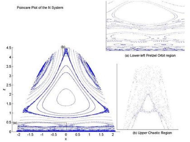
Figure 28: The Poincare plot of the N system. The squares denote the parts of the plot magnified in the insets.

The Poincare section for the N system is shown in fig. 28. There is a fixed point at the centre of the plot surrounded by a subregion of near-integrable curves. All of the annuli are contained within the large triangle surrounding this region; its boundary contains a thin region of chaos, beyond which is the pretzel region.

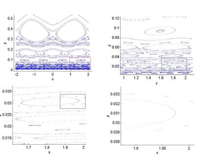
Figure 29: A series of successive close-ups of the lower section of the Poincare plot of the N system. This illustrates the self-similar structure in the pretzel region that repeats at increasingly small scales.  The limiting factor at very small scales is the number of trajectories that we included in the plot.

The structure of the lower part and upper corners of fig. 28 is extremely complicated and intricate, as illustrated by the insets.  The chaotic regions are confined and not simply connected. Though not integrable, the N system shows a high degree of regularity. There is a self-similarity within the pretzel region as illustrated in fig.29, with the circles bounding the quasi-periodic near-integrable regions repeating themselves on increasingly small scales. We find that motions in the N system are completely regular, as evidenced by the absence of dark areas in the Poincare section (except for the one region of chaos mentioned previously). These results are all commensurate with those of the wedge system [13].

We pause here to comment on the symbol sequences corresponding to particular patterns. For example, the two large circles observed just below the annulus region correspond to the boomerang-shaped orbits ($\overline{AB^{3}}$). The next set of circles will be $\overline{A^{2}B^{3}}$, and so on. The collections of crescents between these sets of circles correspond to sequences $\overline{AB^{3}A^{2}B^{3}}$, $\overline{AB^{3}AB^{3}A^{2}B^{3}}$, and so on. Of course, for each circle in the Poincare plot there is in fact a continuum of possible circles, whose diameter depends on the initial conditions. At the center of this family of circles is a dot corresponding to the periodic orbit in question.

Another observable feature in the Poincare plot is a series of closed circles that lie in a triangular pattern in the annulus region. These correspond to quasi-periodic orbits about the periodic annuli with higher period; for example figs. 4, 5 and 6.

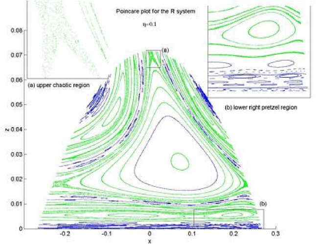
Figure 30: The Poincare plot of the R system at $\eta=0.1$. The right insets provides a close-up of the chaotic region at the top of the diagram; note that it is similar to the N system, but distorted in shape. The left inset is a close-up of the structure in a pretzel region in the lower right of the diagram; it is similarly distorted relative to the N system.

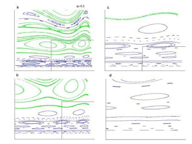
Figure 31: A series of successive close-ups of the lower section of the Poincare plot of the R system at $\eta=0.1$. We see no evidence of a breakdown to chaotic behaviour. Rather the self-similar structure in the pretzel region apparently repeats at increasingly small scales as in the N system.  

Turning next to the R system we find the result that all of the features of its Poincare plot are qualitatively similar to the N system over the range of $\eta$ that we were able to investigate. This is remarkable considering the high degree of non-linearity of the relativistic Hamiltonian given by (55).  The annulus, pretzel and chaotic regions all retain their same basic structure, as seen in fig. 30.

However we find that the plot is no longer symmetric with respect to $p_{R}=0$, and that the Poincare plot is asymmetrically deformed relative to its counterpart in the N system, the deformation increasing with increasing $\eta$, as figs. 30, 32 and 33 illustrate. Superficially this deformation is somewhat puzzling: the trajectories of a subset of the annulus-type orbits always have positive radial velocities when they intersect one of the hexagon’s edges (and the tendency of all annulus orbits is to have $p_{R}>0$ at the bisectors). However it occurs because the Hamiltonian given by eq. (55) is not invariant under the discrete symmetry $p_{i}\rightarrow-p_{i}$, but rather is invariant only under the weaker discrete symmetry $\left(p_{i},\epsilon\right)\rightarrow\left(-p_{i},-\epsilon\right)$.  The parameter $\epsilon=\pm 1$ is a discrete constant of integration that is a measure of the flow of time of the gravitational field relative to the particle momenta.  We have chosen $\epsilon=+1$ throughout, which has the effect of making the principal features of the Poincare plot ‘squashed’ towards the lower right-hand side of the figure relative to its counterpart in the N system. This deformation would be toward the lower-left had we chosen $\epsilon=-1$. It is reminiscent of the situation for two particles, in which the gravitational coupling to the kinetic-energy of the particles causes a distortion of the trajectory from an otherwise symmetric pattern [5, 8], becoming more pronounced as $\eta$ increases.

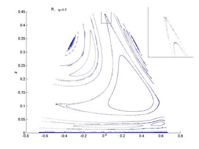
Figure 32: The Poincare plot of the R system at $\eta=0.5$. The right inset provides a close-up of the chaotic region at the top of the diagram. The chaotic region is smaller and the distortion increased relative to the $\eta=0.1$ case. Fewer points appear on this figure because fewer trajectories were run to generate it.

Remarkably we do not find a breakdown from regular to chaotic motion as $\eta$ increases in the R case. The lower regions of the Poincare map clearly display the same patterns of series of circles as occurs in the non-relativistic case and no sizeable connected areas of chaos are present. This is clear from figs. 31 and 34, which respectively show a sequence of successive close-ups of the pretzel region for the $\eta=0.1$ and $\eta=0.75$ cases. However we do find that at $\eta=0.75$ the lines between the near-integrable elliptic regions increases, suggesting either the onset of KAM breakdown or a relativistic generalization of the fractal pattern seen in the N system.  Unfortunately we have not been able to investigate whether or not KAM breakdown occurs for higher $\eta$ values in the R system due to a lack of computer resources.

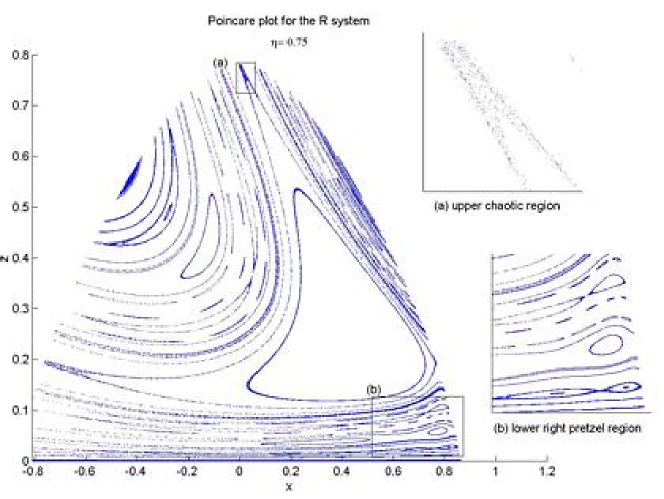
Figure 33: The Poincare plot of the R system at $\eta=0.75$. The upper right inset provides a close-up of the chaotic region at the top of the diagram; it is now considerably narrower than for lower values of $\eta$. The lower-right inset is a close-up of the structure in a pretzel region in the lower right of the diagram. The lines between the various ellipses have slightly thickened, possibly suggesting preliminary stages of KAM breakdown.

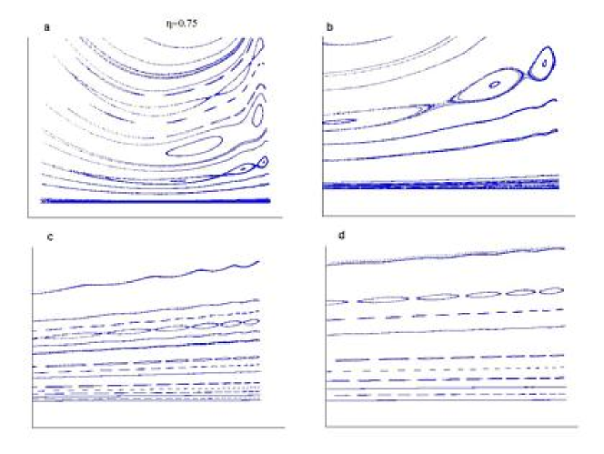
Figure 34: A series of successive close-ups of the lower right section (pretzel region) of the Poincare plot of the R system at $\eta=0.75$. While this region is still highly regular, the lines joining the ellipses are suggestive of the early stages of KAM breakdown, as is the appearance of waviness in the solid lines.  

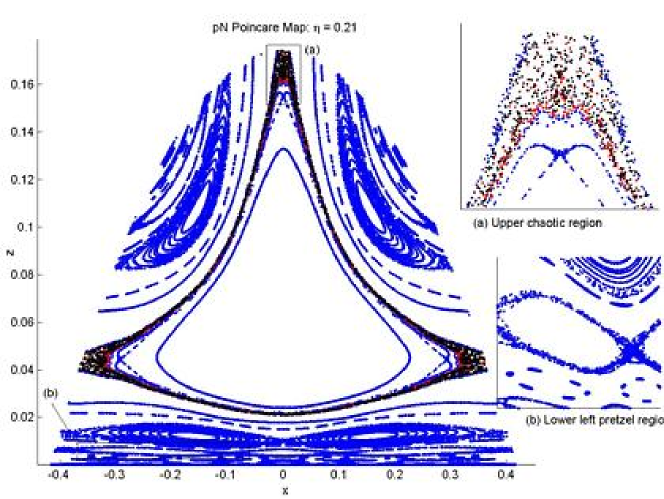
Figure 35: The Poincare plot for the pN system at $\eta=0.21$.  Unlike the R system, it is qualitatively similar to the N system in terms of symmetry. However the chaotic regions have increased in size, with the pretzel region being on the threshold of KAM breakdown.

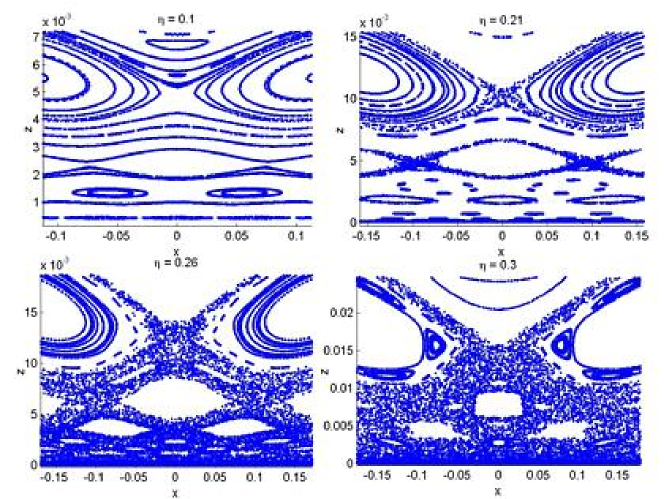
Figure 36: A close-up of the Poincare plots for the pN system for increasing values of $\eta$.  The diagrams are all of the same lower part of the section.  We see clear evidence of KAM breakdown as $\eta$ gets larger.

The pN system has a considerably different Poincare plot, shown in fig. 35.   While it retains the $p_{i}\rightarrow-p_{i}$ symmetry of its N-system predecessor, it appears to undergo a KAM transition from relatively orderly behavior in the N system, to highly chaotic behavior at $\eta=.3$, as the series of Poincare sections in figure 36 demonstrates. At $\eta=.21$, the lines across the bottom of the figure have widened slightly, though the overall behavior is still quite regular. As $\eta$ increases to $.26$, larger regions of chaos become evident around the edges of the groups of ellipses that traverse the lower regions of the figure. At $\eta=.3$, most of the lower section of the Poincare section has been engulfed by a chaotic sea; only a few non-connected islands of regular motion remain. This contrasts sharply with the behavior of the R system at similar values of $\eta$.

The differences between the R and pN cases are not artifacts of the difference in scalings; when trajectories with the same energy are compared, the pN ones are visibly more chaotic than both the N ones and the R ones. The apparent dearth of chaos in the R system is somewhat surprising, as it indicates that most trajectories are effectively restricted to move on two-dimensional surfaces in phase space, as in the N case. This occurs despite the fact that the R system appears not to be integrable (chaotic orbits separating the annulus and pretzel regions do seem to exist) for any $\eta$ within the range investigated. Nonetheless, clearly some underlying feature enforces considerable structure on the phase space– a feature that is absent from the pN system.

8 Discussion

We consider in this section some general features of the motion of the three systems we have studied.

We find for each system that the $\overline{B}$ symbol sequence always occurs, for all values of $\eta$ that we were able to investigate. This leads to a rich variety of annulus diagrams, symmetric about the $\rho=0$ axis for the N and pN systems, but with the axis of symmetry rotated slightly for the R system, the rotation increasing with increasing $\eta$.  We conjecture that $\overline{B}$ motion takes place for arbitrarily large $\eta$ in each of the pN and R systems. It would be interesting to test this conjecture – were it not to hold it would mean that a highly relativistic system must either experience a full KAM breakdown or else repeatedly develop temporary quasi-bound 2-body subsystems.  One thing substantiating this conjecture is that there is no evidence that the annulus region is shrinking with increasing $\eta$ in either the pN or R systems.  However to prove this would require a relativistic equivalent of the discrete mappings for the N case constructed in ref. [13].

We found that the pretzel-type orbits display a remarkable richness of dynamics for all three systems. As the angular momentum of the trajectory in question decreases, the number of successive $A$ collisions increases before the hex-particle sweeps around the origin in the $B^{3}$-sequence.  For example the trajectory $\overline{AB^{3}}$ (the simplest sequence after $\overline{B}$) corresponds to a boomerang-type orbit and appears as two circles on the Poincare section. The next simplest sequence is $\overline{A^{2}B^{3}}$, which corresponds to a bow-tie like orbit, and generates three slightly smaller circles on the Poincare section.

Even in the small region of phase space between these two simple orbits a complex tangle of periodic and quasi-periodic orbits exists. For each of the patterns above, a family of orbits exists corresponding to different widths of the ‘bands’ of phase space that the trajectory covers, and correspondingly different radii of circles in the Poincare section. Between these regions, the orbits’ sequences are mixtures of $AB^{3}$ and $A^{2}B^{3}$. This reasoning can be extended to more general $A^{n}B^{3m}$-motions. We conjecture that the only allowed non-chaotic orbits – relativistic and non-relativistic – are of the form $\prod_{i,j,k}\left(A^{n_{i}}B^{3m_{j}}\right)^{l_{j}}$ with $n_{i},m_{j}$ finite, corresponding to increasingly complex weaving patterns. We expect this conjecture to hold – at least for the range of $\eta$ that we could access numerically – for both the R and N systems (so that the pretzel class can be divided into countably many distinct sub-classes: one for each triple $(n_{i},m_{j},l_{k})$), but not for the pN system, as it experiences KAM breakdown.

If the set of integers $l_{k}$ is finite, then the sequence is regular, leaving bands of phase space untraveled, and appearing as a series of closed crescents or ellipsoids on the Poincare section. If, however, the sequence of integers $l_{k}$ never repeats itself, then the trajectory will fill the available phase space densely, appearing as a wavy line on the surface of section. We conjecture that there is a $1-1$ correspondence between rational numbers and periodic orbits in this region of phase space, both for the N and R systems. This would give the lower section of the Poincare plot a fractal structure as the patterns of circles, ellipses and lines is repeated on arbitrarily small scales as the hex-particle’s angular momentum approaches zero.

9 Conclusions

In (1+1) dimensions the degrees of freedom of the gravitational field are frozen. One therefore expects the motion of a set of $N$ particles in curved spacetime to be described by a conservative Hamiltonian. We find this to be the case for the 3-body system we have studied. By canonically reducing the $N$-body action (2) to first-order form we derived an exact determining equation of the Hamiltonian from the matching conditions. To our knowledge this is the first such derivation for a relativistic self-gravitating system.  The canonical equations of motion given by the Hamiltonian can be explicitly derived from this equation and then numerically solved.

We recapitulate the main results of this paper:

1. We obtained the post-Newtonian expansion of the system we studied, along with its non-relativistic limit.  By comparing these two systems (pN and N respectively) with their relativistic (R) counterpart we were able to study quantitatively the distinctions between each of these systems. There are two spatial degrees of freedom and two conjugate momenta in each, and so the systems are most easily studied by making the transformations (63-65). This yields the hex-particle representation of the system: the 3-body N system is equivalent to that of a single particle moving in a hexagonal linear well.  The pN and R systems distort this well by making the sides concave and convex respectively, with the latter system inducing momentum-dependent changes to its shape.

2. We found that in the equal-mass case each system exhibited the same three qualitative types of motion, that we classified in the hex-particle representation as annulus, pretzel and chaotic.  Annulus orbits correspond to motions in which no two particles ever cross one another twice in succession.  Annuli can be either periodic, quasi-periodic, or densely filled.  Pretzel orbits correspond to motions in which a pair of particles cross each other at least twice before either crosses the third.  This yields a very broad variety of increasingly intricate patterns for each system, dependent upon the initial conditions. Stable bound subsystems of two particles exist for each system. Chaotic orbits have no regular pattern, and correspond to the case when the hex-particle crosses the origin. For energies close to the total rest-energy we find that all of these types of orbits are virtually indistinguishable for each of the N, pN and R systems.

3. We find that differences between each system become more pronounced as $\eta$ increases. In general orbits in the R system are of higher frequency and cover a smaller region of the $\left(\rho,\lambda\right)$ plane than those of its N system counterparts at the same energy.  If the same initial conditions are posed for each system, the motions differ considerably, with the R system having more energy and covering a larger region of the $\left(\rho,\lambda\right)$ plane.  Annulus orbits in the R system have a symmetry axis that is rotated slightly relative to their N and pN counterparts.  Pretzel orbits develop an hourglass shape in the R system that is not seen in the N system, and additional turning points appear for these orbits that are absent in the N system.

4. We find that the qualitative features of the Poincare sections for the R and N systems remain the same for all values of $\eta$ that we were able to study. This is remarkable given the high degree of non-linearity in the former.  However the R system has a weaker symmetry than its N counterpart and so its Poincare section develops an asymmetric distortion that increases with increasing $\eta$.

5. We find that the pN system experiences a KAM breakdown that is not seen in the R and N systems.  This takes place for $\eta\simeq 0.26$: lines separating distinct near-integrable regions become increasingly wider as $\eta$ increases, degenerating into chaos.

A number of interesting questions arise from this work.  First, it would be of considerable interest to explore the R system in the large $\eta$ regime.  This will require considerably more sophisticated numerical algorithms than we have been using that avoid the numerical instabilities we encountered, as well as perhaps employing a time parameter that is not the coordinate time.  Second, an investigation of the unequal mass case should be carried out to see if the common features between the N, R and pN systems are retained. In the N system, when masses are unequal, simply connected regions of global chaos appear; the relationship of these regions to their pN and R counterparts remains a subject for future consideration. Work on the unequal mass case is in progress [24].

APPENDIX A: The Determining equation in hexagonal coordinates

The form of the determining equation is given by (55), and we wish to rewrite it in terms of the four independent degrees of freedom $\left(\rho,\lambda,p_{\rho},p_{\lambda}\right)$, using the relations (65) and (70-72).

Consider first the expressions in the exponentials. Some algebra shows that

$$H_{0} \equiv (L_{1}+{\mathfrak{M}}_{12})z_{13}-(L_{2}+{\mathfrak{M}}_{21})z_{23}$$ (87)

$$= \sqrt{2}H\rho-\epsilon\left(2\left|\rho\right|p_{\rho}+\left[\left|\lambda+\frac{\rho}{\sqrt{3}}\right|-\left|\lambda-\frac{\rho}{\sqrt{3}}\right|\right]p_{\lambda}\right)$$

$$H_{-} \equiv (L_{2}+{\mathfrak{M}}_{23})z_{21}-(L_{3}+{\mathfrak{M}}_{32})z_{31}$$ (88)

$$= H\left(\lambda-\frac{\rho}{\sqrt{3}}\right)-\epsilon\left(\left[\left|\rho\right|-\frac{\sqrt{3}}{2}\left|\lambda+\frac{\rho}{\sqrt{3}}\right|\right]\left(\frac{p_{\lambda}}{\sqrt{3}}+p_{\rho}\right)+\frac{3}{2}\left(p_{\lambda}-\frac{p_{\rho}}{\sqrt{3}}\right)\left|\lambda-\frac{\rho}{\sqrt{3}}\right|\right)$$

$$H_{+} \equiv (L_{3}+{\mathfrak{M}}_{31})z_{32}-(L_{1}+{\mathfrak{M}}_{13})z_{12}$$ (89)

$$= -H\left(\lambda+\frac{\rho}{\sqrt{3}}\right)-\epsilon\left(\left[\left|\rho\right|-\frac{\sqrt{3}}{2}\left|\lambda-\frac{\rho}{\sqrt{3}}\right|\right]\left(\frac{p_{\lambda}}{\sqrt{3}}-p_{\rho}\right)-\frac{3}{2}\left(p_{\lambda}+\frac{p_{\rho}}{\sqrt{3}}\right)\left|\lambda+\frac{\rho}{\sqrt{3}}\right|\right)$$

Writing

$$m_{+}=m_{1}\textrm{, \ }m_{-}=m_{2}\textrm{, }m_{0}=m_{3}\textrm{ \ \ \ \ \ \ \ \ \ \ }s_{\pm}=\frac{\left|\lambda\pm\frac{\rho}{\sqrt{3}}\right|}{\lambda+\frac{\rho}{\sqrt{3}}}\textrm{ \ \ \ \ \ \ }s_{0}=\frac{\left|\rho\right|}{\rho}$$ (90)

we obtain

$$L_{+}L_{-}L_{0}={\mathfrak{M}}_{+-}{\mathfrak{M}}_{-+}L_{0}^{\ast}e^{\frac{\kappa}{4}s_{0}H_{0}}+{\mathfrak{M}}_{-0}{\mathfrak{M}}_{01}L_{+}^{\ast}e^{\frac{\kappa}{4}s_{-}H_{-}}+{\mathfrak{M}}_{0+}{\mathfrak{M}}_{+0}L_{-}^{\ast}e^{\frac{\kappa}{4}s_{+}H_{+}}$$ (91)

where

$$\textrm{\ }M_{0} = \sqrt{\frac{2}{3}}\sqrt{p_{\lambda}^{2}+m_{0}^{2}}\textrm{\ \ \ \ \ \ \ \ \ \ \ }M_{\pm}=\frac{1}{\sqrt{2}}\sqrt{\left(\frac{p_{\lambda}}{\sqrt{3}}\pm p_{\rho}\right)^{2}+2m_{\pm}^{2}}$$ (92)

$$L_{\pm} = H-M_{\pm}\pm\frac{\epsilon}{\sqrt{2}}\left[\left(\frac{p_{\lambda}}{\sqrt{3}}\mp p_{\rho}\right)s_{0}\pm\frac{2}{\sqrt{3}}p_{\lambda}s_{\pm}\right]\textrm{ \ \ \ \ \ }$$ (93)

$$L_{0} = H-M_{0}-\frac{\epsilon}{\sqrt{2}}\left[\left(\frac{p_{\lambda}}{\sqrt{3}}+p_{\rho}\right)s_{+}+\left(\frac{p_{\lambda}}{\sqrt{3}}-p_{\rho}\right)s_{-}\right]$$ (94)

$${\mathfrak{M}}_{\pm\mp} = M_{\pm}\mp\frac{\epsilon}{\sqrt{2}}\left(\frac{p_{\lambda}}{\sqrt{3}}\pm p_{\rho}\right)s_{0},\textrm{ \ \ }{\mathfrak{M}}_{\pm 0}=M_{\pm}-\frac{\epsilon}{\sqrt{2}}\left(\frac{p_{\lambda}}{\sqrt{3}}\pm p_{\rho}\right)s_{\pm}\textrm{\ \ \ \ \ \ \ \ \ }$$ (95)

$$\textrm{\ \ \ \ \ }{\mathfrak{M}}_{0\pm} = M_{o}+\frac{\epsilon\sqrt{2}}{\sqrt{3}}p_{\lambda}s_{\pm}\textrm{\ \ \ \ }L_{0}^{\ast}=(1-s_{+}s_{-})M_{0}+L_{0}$$ (96)

$$L_{\pm}^{\ast} = (1\mp s_{0}s_{\pm})M_{\pm}+L_{\pm}$$ (97)

Acknowledgements

This work was supported by the Natural Sciences and Engineering Research Council of Canada.

References

- [1] G. Rybicki, Astrophys. Space. Sci 14 (1971) 56.
- [2] See B.N. Miller and P. Youngkins, Phys. Rev. Lett. 81 4794 (1998); K.R. Yawn and B.N. Miller, Phys. Rev. Lett. 79 3561 (1997) and references therein.
- [3] H. Koyama and T. Kinoshi, Phys Lett. A (in press; astro-ph/0008208).
- [4] T. Ohta and R.B. Mann, Class. Quant. Grav. 13 (1996) 2585.
- [5] R.B. Mann and T. Ohta, Phys. Rev. D57 (1997) 4723; Class. Quant. Grav. 14 (1997) 1259.
- [6] R.B. Mann, D. Robbins and T. Ohta, Phys. Rev. Lett. 82 (1999) 3738.
- [7] R.B. Mann, D. Robbins and T. Ohta, Phys. Rev. D60 (1999) 104048.
- [8] R.B. Mann, D. Robbins, T. Ohta and M. Trott, Nucl. Phys. B590 367.
- [9] R.B. Mann and T. Ohta, Class. Quant. Grav. 17 (2000) 4059.
- [10] R.B. Mann and P. Chak, Phys. Rev. E65 026128 (2002).
- [11] R.B. Mann, Class.Quant.Grav.18 (2001) 3427.
- [12] R. Kerner and R.B. Mann, gr-qc/0206029.
- [13] H.E. Lehtihet and B.N. Miller, Physica 21D, 93 (1987).
- [14] N. D. Whelan, D. A. Goodings, and J. K. Cannizzo, Phys. Rev. A42, 742 (1990)
- [15] D. Butka, G. Karl and B. Nickel, Can J. Phys 78, 449 (2000).
- [16] V.Millner, J.L.Hanssen, W.C. Campbell, and M.G. Raizen, Phys. Rev. Lett. 86, 1514 (2001).
- [17] R.B. Mann, Found. Phys. Lett. 4 (1991) 425; R.B. Mann, Gen. Rel. Grav. 24 (1992) 433.
- [18] S.F.J. Chan and R.B. Mann, Class. Quant. Grav. 12 (1995) 351.
- [19] R. Jackiw, Nucl. Phys. B 252, 343 (1985); C. Teitelboim, Phys. Lett. B 126, 41, (1983).
- [20] T. Banks and M. O’ Loughlin, Nucl. Phys. B362 (1991) 649; R.B. Mann, Phys. Rev.D47 (1993) 4438.
- [21] T. Ohta and T. Kimura, Phys. Letters 63A (1977) 193; 90A (1982) 389; Progr. Theor. Phys. 68 (1982) 1175.
- [22] V.I. Arnold and A. Avez, Ergodic Problems of Classical Mechanics (Springer: New York, 1968); A. N. Kolmogorov, Dokl. Akad. Nauk. SSSR, 98, 525 (1954) (An English version can be found in Proceedings of the 1954 International Congress of Mathematics, North-Holland, Amsterdam,m 1957); V.I. Arnold, Russ. Math. Surv., 18, 85-191 (1963); J. Moser, Nachr. Akad. Wiss. Goettingen Math. Phys., K1 1 (1962).
- [23] H. Reichl and R. Zheng: NonLinear Resonance and Chaos in Directions in Chaos, (World Scientific 1987) ed. B. Hao.
- [24] J.J. Malecki and R.B. Mann, to appear.