What can the quantum liquid say on the brane black hole, the entropy of extremal black hole and the vacuum energy?

Using quantum liquids one can simulate the behavior of the quantum vacuum in the presence of the event horizon. The condensed matter analogs demonstrate that in most cases the quantum vacuum resists to formation of the horizon, and even if the horizon is formed different types of the vacuum instability develop, which are faster than the process of Hawking radiation. Nevertheless, it is possible to create the horizon on the quantum-liquid analog of the brane, where the vacuum life-time is long enough to consider the horizon as the quasistationary object. Using this analogy we calculate the Bekenstein entropy of the nearly extremal and extremal black holes, which comes from the fermionic microstates in the region of the horizon – the fermion zero modes. We also discuss how the cancellation of the large cosmological constant follows from the thermodynamics of the vacuum.

1 Introduction

In general relativity the event horizon is a rather fragile construction: small deviations from Einstein theory leads to the catastrophical consequence for the event horizon. In particular, the horizon is destroyed: (i) after inclusion of arbitrarily small mass terms for graviton [1]; (ii) after inclusion of higher order curvature terms [2]; (iii) in the models allowing varying speed of light [3]; etc. Thus there is an open question whether the horizon can be really formed.

The condensed matter analogs of gravity also indicate that the event horizon for quasiparticles is a subtle issue: in most systems it cannot be formed. The characteristic example is the black-hole horizon for sound waves generated by a moving liquid as suggested by Unruh [4]. The horizon for sound waves can be formed when the local velocity of the liquid exceeds the speed of sound. In liquids, however, the effective metric experienced by sound waves obeys the hydrodynamic equations which thus play the role of Einstein equations, and these hydrodynamic equations prohibit the existence of the spherically symmetric event horizon [5]. The horizon can be formed only in the vessels of special geometry such as the so-called Laval nozzle [6]. However, even in this case the horizon will be spoiled by the formation of shock waves.

The constraints dictated by the hydrodynamic equations can be avoided if one constructs the horizon for such quasiparticles whose maximum attainable speed $c$, which plays the role of the ‘speed of light’, is smaller than the speed of sound. In this case the speed of sound is not reached at the quasiparticle horizon, and thus the horizon is not accompanied by the hydrodynamic instability. Such situation can occur, for example, in superfluids ³He-A where the superfluid ground state plays the role of the quantum vacuum, while some low-frequency bosonic collective modes of the superfluid vacuum mimic the effective gravitational field experienced by the ‘relativistic’ quasiparticles – the Weyl fermions [7]. In this superfluid liquid the effective gravity is very similar to the Sakharov gravity [8] induced by quantum fluctuations of the vacuum.

In ³He-A the ‘speed of light’ $c$ is about three order of magnitude smaller than the speed of sound. Nevertheless the other instability becomes important – the instability of the superfluid quantum vacuum when it moves with supercritical velocity, $v>c$. This brings us to the problem of the stability of the quantum vacuum in the presence of the non-trivial metric field. After the first proposal by Unruh there were many projects in condensed matter and optics to simulate the event horizon (see the book [9]). Till now we were not able to construct, even in the gedanken experiment, the condensed matter system whose vacuum state remains stable in the presence of the horizon. Who knows, maybe this is an indication that the real quantum vacuum – the ether – is also highly sensitive to the presence of the horizon or ergoregion.

However, recently it was found that there exists a real and experimentally accessible system where the vacuum instability will be developed rather slowly, so that we can investigate the behavior of the vacuum in the presence of the horizon. This is the horizon constructed for quasiparticles living in the analog of the brane – the 2+1 world of the interface between two bulk superfluid vacua, superfluid ³He-A and superfluid ³He-B, which we refer to as the AB-brane. In this situation the hydrodynamic equations determine the flow of two superfluids in bulk, and the velocities of this flow near the AB-brane dictate the effective metric for quasiparticles living on the brane – the ripplons – which play the role of the brane matter. The maximum attainable velocity $c$ for the ripplons is typically much smaller than any critical velocity for the instability of the bulk superfluids. As a result, the ergoregion and the event horizon can be easily constructed without any instability in the bulk liquids.

While the bulk vacuum remains stable, the brane vacuum is nevertheless unstable beyond the horizon. This instability occurs due to the interaction of quasiparticles living on the brane with that living in the bulk liquid (i.e. in the higher-dimensional space outside the brane) which leads to the decay of the brane vacuum in the region behind the horizon. The weaker is the interaction the longer the black hole lives. This mechanism of the vacuum decay can be applicable for the astronomical black holes, if we really live on brane of the higher-dimensional world. If the matter fields on the brane are properly coupled to, say, gravitons in the bulk, this may lead to the collapse of the black hole which is fast as compared to the popular mechanism of the black-hole evaporation by the Hawking radiation [10]. This is another example of the fragility of the horizon, now due to the interaction with the higher-dimensional world. We shall consider this example in Section 2.

If the time of the collapse of the black-hole horizon is long enough, we can study the thermodynamics related to the horizon: its temperature and the Bekenstein entropy. In condensed matter systems, as well as in quantum vacuum, the low-temperature thermodynamic properties of the system is determined by zero modes, fermionic or/and bosonic. If the condensed matter system has no zero modes, the gapless (massless) modes necessarily appear in the presence of the ergoregion or event horizon. In such systems, all the entropy comes from the microstates in the black hole interior or in the vocinity of the horizon, where the fermion zero modes provide the source of the Bekenstein entropy [11]. In Section 3 we consider here the simplest example of the entropy produced by the condensed-matter analog of the extremal black hole.

The condensed matter examples demonstrate that the effective gravity can essentially differ from the fundamental gravity even in principles. For example, in the effective gravity the effective spacetime can be geodesically incomplete. This is simply because the description of the quasiparticle motion in terms of the metric field is incomplete. The effective gravity appears only in the low-energy corner: the general covariance and Einstein equations even if they were valid at low energy, are violated at high energy. The quasiparticle thus can simply leave the low-energy world and enter the non-symmetric high-energy world where the quasiparticle trajectories are governed by the non-relativistic and non-covariant laws.

Since in the effective gravity the general covariance is lost at high energy, the metrics which for the low-energy observers look as equivalent, since they can be transformed to each other by coordinate transformation, are not equivalent physically. Moreover, the vacuum can be essentially different for different metrics which are formally equivalent. If our gravity is also effective, we can in principle resolve between the formally equivalent metrics if we will be able to reach the high enough energy. For example, the Painlevé-Gullstrand [12], Schwarzschild and other metrics used for description of the black hole could be discriminated on physical ground. It is interesting that in the moving superfluids the effective metric which describes the event horizon is of the Painlevé-Gullstrand type where the time reversal symmetry is violated. That is why we shall also use such a type of the metric field for calculations of the Bekenstein entropy related to a horizon. The event horizon which emerge in stationary superfluids and which simulates the Schwarzschild black hole is discussed in [13].

We will be interested here mainly in the entropy of the extremal black hole, in particular because there is a contradiction between different approaches to the calculations of the entropy of such a hole. While the Bekenstein entropy of the Reissner-Nordström black hole in the limit of the extreme hole is proportional to the area of the horizon, ${\cal S}=\pi r_{+}^{2}p_{0}^{2}/\hbar^{2}$, where $p_{0}$ is the Planck momentum, the entropy of the exactly extremal black hole is zero according to [14, 15]. Such a huge jump under any small change of the extremal hole towards the non-extremal one is rather problematic (see discussion in [16]). We consider this problem using the effective gravity and the natural regularization which comes from the non-relativistic Planckian physics of quantum liquids at high energy. We find that the Planckian physics modifies the black hole entropy and smoothens the discontinuity occuring in the limit of the extremal black hole. It happens that for the calculations of the entropy of the extremal or nearly extremal black holes it is not necessary to know the quasiparticle spectrum in the trans-Planckian region: the regularization occurs already at low energy where it is enough to use only the first (cubic) correction to the linear relativistic spectrum: $E(p)\approx cp(1+p^{2}/p_{0}^{2}+\ldots)$.

The thermodynamic approach is also useful for discussion of the condensed matter analogs of the cosmological constant problems (the detailed discussion can be found in the book [7]). In quantum liquids these problems are essentially the same as in our quantum vacuum, with probably the only difference that in the quantum liquids the structure of the quantum vacuum is well known even in the trans-Planckian region. In Section 4 we discuss how the cosmological constant problems (why it is not huge, why it is not zero and why it is on the order of the energy density of matter) are solved in quantum liquids. The solution does not depend on the details of the structure of the quantum liquid and follows from the thermodynamic relation – the Gibbs-Duhem relation – applied to the quantum vacuum as a medium.

2 Black hole on brane

2.1 Simulation of Painlevé-Gullstrand metric

Let us start with the modification of the Unruh dumb hole [4] to superfluids. The effective metric experienced by bosonic or fermionic quasiparticles moving in the background of the superfluid vacuum which flows with the velocity ${\bf v}({\bf r})$ is

$$ds^{2}=-dt^{2}+{1\over c^{2}}\left(d{\bf r}-{\bf v}({\bf r})dt\right)^{2}+{1\over c^{2}}r^{2}d\Omega^{2}~{}.$$ (1)

Here $c$ is the maximum attainable speed of the low-energy quasiparticle. If one considers the radial flow of the superfluid vacuum with the following velocity field

$${\bf v}({\bf r})=\pm\hat{\bf r}c\sqrt{r_{h}\over r}~{},~{}r_{h}={2MG\over c^{2}}~{},$$ (2)

one obtains the metric corresponding to the Painlevé-Gullstrand spacetime describing the gravitational field produced by the point source of mass $M$. At $r=r_{h}$ where the flow velocity reaches $c$ one has the black hole horizon in the case of the vacuum flowing inward (sign -) and the white hole horizon in the case of the flow outward (sign +) [4, 17]). In superfluids, a flow of the superfluid vacuum violates the time-reversal symmetry: the time reversal operation reverses the direction of flow, $T{\bf v}=-{\bf v}$, and thus transforms the black hole into the white one.

The Painlevé-Gullstrand type metric describes the space-time both in exterior and interior regions, and this spacetime, though not static, is stationary. That is why it has many advantages (see [18, 19, 20]), and in particular these properties of the Painlevé-Gullstrand metric allow us to discuss the behavior of the quantum vacuum in the interior of the black hole.

For many reason the radial flow with horizon cannot be realized in normal liquids and also in superfluids, as well as many other flow field configurations suggested for the condensed matter simulation of horizons. Here we discuss the most realistic situation, when the pair of white-hole and black-hole horizons can be formed in quantum liquids and they can live for reasonably long time. This scenario of formation of horizons is based on recent experiments with two superfluids sliding along each other [21, 22].

2.2 Simulation of horizons and physical singularities on brane

In an applied gradient of magnetic field two superfluids, ³He-A and ³He-B, are separated by the AB-brane. They can move without any dissipation along the brane with different velocities ${\bf v}_{1}$ and ${\bf v}_{2}$. Thes velocities are determined in the container frame where the flow field is stationary. From the hydrodynamic equations it follows that that the quasiparticles living on AB-brane – the surface waves called ripplons – have the following dispersion relation if the container has the form of a thin slab

$$\alpha_{1}(\omega-{\bf p}\cdot{\bf v}_{1})^{2}+\alpha_{2}(\omega-{\bf p}\cdot{\bf v}_{2})^{2}=$$

$$=c^{2}p^{2}\left(1+{p^{2}\over p_{0}^{2}}\right)-2i\Gamma(p)\omega,$$ (3)

where

$$\alpha_{1}=\frac{h_{2}\rho_{1}}{h_{2}\rho_{1}+h_{1}\rho_{2}}~{},~{}\alpha_{2}=\frac{h_{1}\rho_{2}}{h_{2}\rho_{1}+h_{1}\rho_{2}}~{},~{}\alpha_{1}+\alpha_{2}=1~{},$$ (4)

$$p_{0}^{2}={F\over\sigma},~{}~{}~{}c^{2}=F{h_{1}h_{2}\over\rho_{1}h_{2}+\rho_{2}h_{1}}~{}.$$ (5)

Here $\sigma$ is the surface tension of the AB-brane; $F$ is the force stabilizing the position of the brane – an applied magnetic-field gradient (see Ref. [21]); $\rho_{1}$ and $\rho_{2}$ are mass densities of the liquids; $h_{1}$ and $h_{2}$ are thiknesses of the layeres of A and B phases, and we assume the ‘shallow water’ condition $ph_{1}\ll 1$ and $ph_{2}\ll 1$; finally $\Gamma(p)$ is the coefficient in front of the friction force experienced by the AB-brane when it moves with respect to the 3D environment along the normal. This friction term which couples the 2D brane with the 3D environment violates Galilean invariance in the 2D world of the AB-brane. In the low-energy effective theory this term is responsible for the violation of the Lorentz invariance in the brane world caused by the interaction with the higher dimensional environment.

For $p\ll p_{0}$ the main part of Eq. (3) can be rewritten in the Lorentzian form

$$g^{\mu\nu}p_{\mu}p_{\nu}=2i\omega\Gamma(p)-c^{2}p^{4}/p_{0}^{2},$$ (6)

$$p_{\mu}=(-\omega,p_{x},p_{y}),~{}~{}~{}p=\sqrt{p_{x}^{2}+p_{y}^{2}},$$ (7)

while the right-hand side of Eq.(6) contains the remaining small terms violating Lorentz invariance – attenuation of ripplons due to the friction and their nonlinear dispersion. Both terms come from the physics which is ‘trans- Planckian’ for the ripplons. The quantities $p_{0}$ and $cp_{0}$ play the role of the Planck momentum and Planck energy within the brane: they determine the scales where the Lorentz symmetry is violated. The Planck scales of the 2D physics in brane are actually much smaller than the ‘Planck momentum’ and ‘Planck energy’ in the 3D superfluids outside the brane. The function $\Gamma(p)$ is determined by the physics of quasiparticles living in bulk which scatter on the brane.

At sufficiently small $p$ both non-Lorentzian terms – attenuation and nonlinear dispersion on the right-hand side of Eq.(6) – can be ignored, and the dynamics of ripplons living on the AB-brane is described by the following effective contravariant metric $g^{\mu\nu}$:

$$\begin{array}[]{c}g^{00}=-1,~{}~{}~{}g^{0i}=-\alpha_{1}v_{1}^{i}-\alpha_{2}v_{2}^{i},\\[2.84526pt] g^{ij}=c^{2}\delta^{ij}-\alpha_{1}v_{1}^{i}v_{1}^{j}-\alpha_{2}v_{2}^{i}v_{2}^{j}.\end{array}$$ (8)

Introducing relative velocity ${\bf U}$ and the mean velocity ${\bf v}$ of two superfluids:

$${\bf v}=\alpha_{1}{\bf v}_{1}+\alpha_{2}{\bf v}_{2},~{}~{}{\bf U}=\sqrt{\alpha_{1}\alpha_{2}}\left({\bf v}_{1}-{\bf v}_{2}\right),$$ (9)

one obtains the following expression for the effective contravariant metric

$$g^{00}=-1~{},~{}~{}g^{0i}=-v^{i}~{}~{},~{}~{}g^{ij}=c^{2}\delta^{ij}-v^{i}v^{j}-U^{i}U^{j}~{}.$$ (10)

The interval of the effective 2+1 spacetime where ripplons move along geodesic curves is

$$ds^{2}=g_{\mu\nu}dx^{\mu}dx^{\nu}=$$

$$-~{}dt^{2}\left(1-{v^{2}\over c^{2}}-{({\bf U}\cdot{\bf v})^{2}\over c^{2}(c^{2}-U^{2})}\right)-~{}2dt\left({{\bf v}\cdot d{\bf r}\over c^{2}}+{({\bf U}\cdot d{\bf r})({\bf U}\cdot{\bf v})\over c^{2}(c^{2}-U^{2})}\right)$$

$$+{d{\bf r}^{2}\over c^{2}}+{({\bf U}\cdot d{\bf r})^{2}\over c^{2}(c^{2}-U^{2})}~{}.$$ (11)

If $U=0$, the two superfluids move with the same velocity and thus can be represented as a single liquid, as a result the Eq.(1) is restored. But in the general case (11) the system is richer than in the case of a single liquid. In principle all the interesting 2+1 metrics can be constructed using two velocity fields. In particular, the ergosurface (which is the ergoline in the 2+1 system) is obtained when

$$g_{00}=0~{}~{},~{}~{}{\rm or}~{}~{}{v^{2}\over c^{2}}+{({\bf U}\cdot{\bf v})^{2}\over c^{2}(c^{2}-U^{2})}=1~{},$$ (12)

and the physical singularity is obtained at $U=c$ where the determinant of the metric

$$g=-{1\over c^{2}(c^{2}-U^{2})}$$ (13)

changes sign. In the particular case when ${\bf U}\perp{\bf v}$ and $v<U$, the singularity at $U=c$ is naked violating the ‘cosmic censorship’ in quantum liquids.

The arrangement of the planned experiment will be similar to that suggested by Schützhold and Unruh [23]. The A and B vacua with the AB-brane between them are confined in the channel. The shape of the cross-section of the channel is such that in the rotating cryostat the superflluid velocities are inhomeheneous as is shown in the Figure 1. In the typical situation the A-phase is at rest in the container frame, while the B-phase is at rest in the inertial frame, which means that ${\bf U}={\bf v}=\hat{\bf\phi}v(\phi)$ and the interval of the effective 2+1 spacetime in which ripplons move along the geodesic curves is given by

$$ds^{2}=-d\tilde{t}^{2}{c^{2}-2v^{2}(\phi)\over c^{2}-v^{2}(\phi)}+{r^{2}d\phi^{2}\over c^{2}-2v^{2}(\phi)}+dr^{2}~{},$$ (14)

$$d\tilde{t}=dt+{v(\phi)rd\phi\over c^{2}-2v^{2}(\phi)}~{}.$$ (15)

In this geometry there are two horizons, the black-hole and white-hole, at points where $v^{2}_{\rm hor}=c^{2}/2$ and thus $g_{00}=0$. The physical singularities occur at points where $v^{2}_{\rm singularity}=c^{2}$ and thus $g_{00}=\infty$ (see Figure 1).

2.3 Vacuum instability due to interaction with bulk

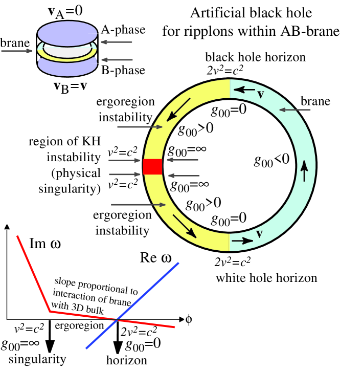
Figure 1: The AB-brane – the ring-shaped interface between two bulk quantum vacua. The coordinate singularities in the effective metric for ripplons living on brane occur at two lines where $v^{2}=c^{2}/2$ and thus $g_{00}=0$. These two lines represent the black-hole and white-hole horizons. The physical singularities occur at two lines where $v^{2}=c^{2}$ and thus $g_{00}=\infty$. Bottom left: real and imaginary parts of the ripplon spectrum. At the horizons both of them change sign. The attenuation of ripplons outside the horizons transforms to the amplification beyond the horizon, which means that the quantum vacuum becomes unstable in the interior of the black hole, and as a result the interior region shrinks. If the interaction with the bulk environment is weak, the vacuum beyond the horizon is long lived, and the physical singularity can be also reached and investigated.

The important feature of the brane physics is the interaction of the brane matter (ripplons) with the bulk world. In the superfluid ³He this interaction gives rise to the imaginary part of the spectrum of brane quasiparticles in Eq.(6): the energy of ripplons has a finite dissipation rate. In the presence of a horizon the situation changes drastically: When the horizon is crossed and the real part of the quasiparticle energy changes sign according to Eq.(6), the imaginary part of the spectrum also changes sign (see Figure 1 bottom left). This means that the attenuation of perturbations which occurs outside the horizon transforms to the amplification of perturbations beyond the horizon, i.e. due to the interaction with the bulk environment the quantum vacuum of the brane becomes unstable in the interior region of the black hole. This instability finally leads to the shrinking of the interior region.

In superfluid ³He the rate of the brane vacuum decay is determined both by the brane and bulk parameters:

$${1\over\tau}\sim\Gamma(p)\sim p^{2}{c_{\rm bulk}T^{3}\over p_{\rm brane}E_{\rm bulk}^{3}}~{},$$ (16)

where $T$ is the temperature in the bulk; $c_{\rm bulk}$ is the maximum attainable speed for quasiparticles living in bulk; $E_{\rm bulk}$ is the Planck energy scale in bulk; and $p_{\rm brane}=p_{0}$ is the brane Planck momentum. Typically the bulk parameters are much larger than that on the brane: $c_{\rm bulk}\gg c_{\rm brane}$; $p_{\rm bulk}\gg p_{\rm brane}$; and $E_{\rm bulk}\gg E_{\rm brane}\equiv c_{\rm brane}p_{\rm brane}=cp_{0}$.

In the current experiments with the AB-brane [21], the shallow water conditions are not satisfied, and thus the ripplons are non-relativistic and are not described by the effective metric. That is why the horizon was not simulated in these experiments. However, the notion of the ergoregion – the region where the ripplons have negative energy in the container frame – is well defined even for the non-relativistic case. The Figure 1 bottom left properly describes the spectrum of the non-relativistic ripplons too, if one substitutes the horizons by the ergosurfaces. The physical singularity corresponds to the points where the Kelvin-Helmholtz instability takes place. The vacuum decay in the ergoregion occurs essentially in the same way as beyond the horizon, and the experimental data for the threshold of the ergoregion instability are in an excelent agreement with the theory. Thus the non-relativistic analog of the discussed mechanism of the brane vacuum decay due to the interaction with the higher-dimensional environment has been experimentally confirmed.

Something similar can occur for the astronomical black holes if we live on the brane of the multidimensional world. The interaction of our brane matter with the bulk environment can lead to the decay of the quantum vacuum beyond the black hole horizon. The time of $\tau$ of the decay depends on the ratio of the bulk and brane parameters, and in principle, this time can be shorter that the quantum process of the black hole evaporation introduced by Hawking. The goal of the future experiments with the AB-brane is to study the vacuum decay in the relativistic regime when the horizon is developed, and at low temperature where the decay time is long, so that the other processes of the vacuum decay become relevant, such as the Corley–Jacobson lasing scenario [24] which occurs in the presence of the pair of horizons.

3 Entropy of extremal black hole

3.1 Simulation of extremal and nearly extremal black holes

In previous Section it was shown that the event horizon for the relativistic quasiparticles can be constructed in quantum liquids at least in principle. Since the microstates of the quantum liquids are well known we can study the problem of the thermodynamics in the presence of the horizon.

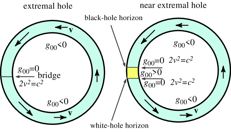
Figure 2: Right: When the black and white horizons in Fig. 1 are close to each other the metric becomes similar to that of the nearly extremal hole. Left: When the two horizons merge the effective metric corresponds to that of the extremal black hole.

When the two horizons are close to each other (Figure 2 right) the quasiparticle interval in Eq.(14) becomes

$$ds^{2}=-d\tilde{t}^{2}(\phi^{2}-\phi_{\rm hor}^{2})+{r^{2}d\phi^{2}\over\phi^{2}-\phi_{\rm hor}^{2}}+dr^{2}~{}.$$ (17)

When the two horizons merge (Figure 2 left) one has $\phi_{\rm hor}^{2}=0$, and the interval becomes

$$ds^{2}=-d\tilde{t}^{2}\phi^{2}+{r^{2}d\phi^{2}\over\phi^{2}}+dr^{2}~{},$$ (18)

One can compare this with the interval for matter in the presence of the Reissner-Nordström black hole of mass $M$ and electric charge $Q$

$$ds^{2}=-d\tilde{t}^{2}{(r-r_{+})(r-r_{-})\over r^{2}}+dr^{2}{r^{2}\over(r-r_{+})(r-r_{-})}+r^{2}d\Omega~{},$$ (19)

$$r_{+}r_{-}=Q^{2}~{},~{}r_{+}+r_{-}=2MG~{},$$ (20)

where $r_{+}$ and $r_{-}$ are external and inner horizons. For the nearly extremal black hole, the two horizons are close to each other, $r_{+}-r_{-}\ll r_{+}+r_{-}\equiv 2r_{h}$. Introducing the coordinate $\tilde{r}=r-(r_{+}+r_{-})/2$ in the vicinity of horizons and the quantity $\tilde{r}_{h}^{2}=(r_{+}-r_{-})^{2}/4$ one obtains

$$ds^{2}\approx-d\tilde{t}^{2}{\tilde{r}^{2}-\tilde{r}_{h}^{2}\over r_{h}^{2}}+d\tilde{r}^{2}{r_{h}^{2}\over\tilde{r}^{2}-\tilde{r}_{h}^{2}}+r_{h}^{2}d\Omega~{},$$ (21)

Thus close to the horizons the radial part of the Reissner-Nordström metric is similar to the azimuthal part of the quasiparticle metric in Eq. (17). When the two horizons merge, i.e. when $\tilde{r}_{h}=0$, one obtains the metric of the extremal hole

$$ds^{2}\approx-d\tilde{t}^{2}{\tilde{r}^{2}\over r_{h}^{2}}+d\tilde{r}^{2}{r_{h}^{2}\over\tilde{r}^{2}}+r_{h}^{2}d\Omega~{},$$ (22)

which is thus simulated by the quasiparticle interval in Eq.(18). Since the thermodynamics of the nearly extremal and the extremal holes are determined by the microstates in the vicinity of the horizons, the difference between the metrics in Eqs.(21–22) and their quasiparticle counterparts in Eqs.(17–18) is not important.

The above examples demonstrate that in principle it is possible to simulate different types of horizons in quantum liquids. Let us now assume that we can construct in a quantum liquid the following effective metric for the ‘relativistic’ quasiparticles:

$$ds^{2}={1\over b(r)}\left[-c^{2}(r)dt^{2}+\left(dr-v(r)dt\right)^{2}\right]+r^{2}d\Omega^{2}=$$ (23)

$$={1\over b(r)}\left[-(c^{2}(r)-v^{2}(r))d\tilde{t}^{2}+dr^{2}{c^{2}(r)\over c^{2}(r)-v^{2}(r)}\right]+r^{2}d\Omega^{2}~{},$$ (24)

$$d\tilde{t}=dt+{v(r)dr\over c^{2}(r)-v^{2}(r)}~{}.$$ (25)

Here $v(r)$ is the velocity of the radial flow of the liquid; $c(r)$ is the local maximum attainable speed of the relativistic quasiparticle in the reference frame comoving with the liquid; and $b(r)$ is some function related to the local density of the liquid. One can check that the metric in Eq.(24) coincides with the metric of Reissner-Nordström black hole of mass $M$ and electric charge $Q$ in Eq.(19) if one chooses

$$b(r)={c(r)\over c}=1+{Q^{2}\over r^{2}}~{}~{},~{}~{}v(r)=-\sqrt{2GMb(r)\over r}~{}~{},~{}~{}c=c(r=\infty)~{}.$$ (26)

The quasiparticle metric in Eq.(23) is thus the analog of the Painlevé-Gullstrand metric describing the spacetime both in exterior and interior regions of the Reissner-Nordström black hole.

3.2 Fermi surface in the interior of nearly extremal black hole

The spacetime in Eq.(23), though not static, is stationary. That is why the quasiparticle energy spectrum in the interior region is well determined. It has the form of Eq.(6)

$$g^{\mu\nu}p_{\mu}p_{\nu}+m^{2}+c^{2}p^{4}/p_{0}^{2}=0~{},$$ (27)

where the effective Painlevé-Gullstrand metric $g^{\mu\nu}$ is given by Eq.(23), and we neglected the possible interaction of quasiparticles with the environment which leads to the broadening of the spectrum. The dispersion relation (27) contains only the first non-linear correction to the relativistic spectrum which violates the Lorentz symmetry. Though the main contribution to the thermodynamics of the black hole comes from the short wave length, where the Planck physics intervenes, it happens that for the nearly extremal and extremal holes only this first correction is important, while the higher-order terms can be neglected. Thus one has the following quasiclassical energy spectrum $E({\bf p})$ in the background of the Reissner-Nordström black hole:

$${1\over b(r)}\left(E-p_{r}v(r)\right)^{2}=b(r)c^{2}p_{r}^{2}+c^{2}p_{\perp}^{2}+m^{2}+{p^{4}\over p_{0}^{2}}~{}.$$ (28)

where $p_{r}$ is the radial momentum of the (quasi)particle and $p_{\perp}$ is its transverse momentum.

We are interested in the spectrum of fermionic quasiparticles, since according to the quantum liquid analogy for the quantum vacuum only the fermions are fundamental while the bosons appear as collective modes of the quantum vacuum [7]. In the Standard Model these quasiparticles correspond to $N_{F}=16N_{g}$ chiral fermionic species where $N_{g}$ is the number of generations. The most important property of the fermionic spectrum in the presence of the horizons is the existence of the Fermi surface, which appears even for fermions with nonzero mass $m$: the Fermi surface appears at large momentum $p$ where the mass term can be neglected. Fermi surface is the 2D surface in the 3D momentum space, where the energy of the particle is zero: $E({\bf p})=0$. For the spectrum in Eq.(28) this 2D manifold of fermion zero modes is given by equation, which expresses the radial momentum in terms of the transverse momentum $p_{\perp}$ (we put $c=1$):

$$p_{r}^{2}(p_{\perp})={1\over 2}p_{0}^{2}\left({v^{2}\over b}-b\right)-p_{\perp}^{2}\pm\sqrt{{1\over 4}p_{0}^{4}\left({v^{2}\over b}-b\right)^{2}+p_{0}^{2}p_{\perp}^{2}\left(b-1-{v^{2}\over b}\right)}~{}.$$ (29)

This surface exists at each point ${\bf r}$ between the horizons, where $v^{2}>b^{2}$. It exists only in the restricted range of the transverse momenta, with the restriction provided by the parameter $p_{0}$ which plays the role of the Planck momentum:

$$p_{\perp}^{2}<{1\over 4}p_{0}^{2}{(v^{2}-b^{2})^{2}\over b^{2}-b^{3}+bv^{2}}~{}.$$ (30)

This means that the Fermi surface is a closed surface in the 3D momentum space ${\bf p}$.

3.3 Entropy of nearly extremal black hole

The main thermodynamic property of the fermion zero modes with the Fermi surface is that its vacuum is characterized by a finite density of fermionic states (DOS) $N(E=0)$. For each of $N_{F}=16N_{g}$ fermionic species the DOS is:

$$N(E)=\sum_{{\bf p},{\bf r}}\delta(E({\bf p})-E)~{},$$ (31)

$$N(E=0)={4\pi\over(2\pi)^{3}}\int_{r_{-}}^{r_{+}}r^{2}dr\int d^{3}p~{}\delta(E({\bf p}))={1\over\pi}\int_{r_{-}}^{r_{+}}r^{2}dr\int_{0}^{p_{\perp}^{2}(r)}{d(p_{\perp}^{2})\over|v_{G}|}~{},$$ (32)

where $v_{G}$ is the radial component of the group velocity of (quasi)particles at the Fermi surface:

$$v_{G}(E=0,p_{\perp},r)={dE\over dp_{r}}\big{|}_{E=0}=\mp{1\over v}\sqrt{(v^{2}-b^{2})^{2}+4{p_{\perp}^{2}\over p_{0}^{2}}(b^{3}-b^{2}-bv^{2})}~{}.$$ (33)

Integration over $p_{\perp}^{2}$ in Eq.(32) gives for the DOS

$$N(E=0)={p_{0}^{2}\over\pi}\int_{r_{-}}^{r_{+}}r^{2}dr{|v|(v^{2}-b^{2})\over bv^{2}+b^{2}-b^{3}}~{}.$$ (34)

In the extreme limit $Q\rightarrow M$ one obtains

$$N(E=0)\approx{4\over 3\pi}p_{0}^{2}r_{+}^{3}\left(1-{Q^{2}\over M^{2}}\right)^{3/2}~{}.$$ (35)

Let us emphasize that the (quasi)particles contributing to this DOS live between the two horizons, i.e. $r_{-}<r<r_{+}$. The characterisic momenta of these (quasi)particles are $p\sim p_{0}\sqrt{1-{Q^{2}\over M^{2}}}$. In the extreme-hole limit these momenta, though much larger than any fermionic mass, are still much smaller than the Planck momentum $p_{0}$. This is the reason why in this limit only the first non-linear correction to the relativistic spectrum in Eq.(27) is relevant.

At non-zero temperature the fermionic microstates forming the Fermi surface give the following Bekenstein entropy:

$${\cal S}(T,M,Q)={\pi^{2}\over 3}N(E=0)T=4\pi N_{F}{p_{0}^{2}r_{+}^{3}T\over\hbar^{3}c}\left(1-{Q^{2}\over M^{2}}\right)^{3/2}~{},$$ (36)

which is linear in $T$.

3.4 Entropy of extremal black hole

For the extremal black hole ($Q=M$) the two horizons merge and the Fermi surface disappears. As a result the linear in $T$ term in Eq.(36) for the Bekenstein entropy becomes zero. This means that the entropy of the extremal black hole must be of higher order in $T$. Let us calculate this entropy. It can be obtained directly from the thermal energy

$${\cal E}=\int dEEN(E)f(E/T)=\sum_{{\bf p},{\bf r}}E({\bf p},{\bf r})f(E({\bf p},{\bf r})/T)~{},$$ (37)

where $f$ is the Fermi distribution function. For the extremal hole one has $b^{2}(r)-v^{2}(r)\approx 2(r-r_{+})^{2}/r_{+}^{2}$, and after the change of variables

$${p_{r}(r-r_{+})^{2}\over 2r_{+}^{2}}=x^{2}~{}~{},~{}~{}{p_{\perp}^{2}\over 2p_{r}}=y^{2}~{}~{},~{}~{}{p^{3}_{r}\over 2p_{0}^{2}}=z^{2}~{},~{}E=x^{2}+y^{2}+z^{2}=u^{2}~{},$$ (38)

one obtains the following dependence of the DOS on $E$

$$N(E)dE={d^{3}rd^{3}p\over(2\pi)^{3}}={2\over\pi}dp_{r}~{}d(p_{\perp}^{2})~{}r^{2}dr={1\over 3\pi}p_{0}r_{+}^{3}|u|d^{3}u={2\over 3c^{2}}p_{0}r_{+}^{3}EdE~{}.$$ (39)

Thus the DOS of fermion zero modes living at the extremal black hole is equivalent to the DOS of the 2D relativistic gas of massless fermions with zero chemical potential, whose density of states is $N(E)=(2/3)p_{0}r_{+}^{3}E$. The entropy of such gas and thus the entropy of extremal black hole is

$${\cal S}_{\rm extremal~{}hole}=3\zeta(3)N_{F}{p_{0}r_{+}^{3}\over c^{2}\hbar^{3}}T^{2}~{}.$$ (40)

The entropy in Eq.(36) for the nearly extremal black hole which is valid for

$$1\gg 1-{Q^{2}\over M^{2}}\gg\left({T\over cp_{0}}\right)^{2/3}~{},$$ (41)

smoothly transforms to the entropy in Eq.(40) for the extremal black hole, when the parameter $1-{Q^{2}\over M^{2}}$ approaches $(T/cp_{0})^{2/3}$.

Let us stress again that for the extremal black hole the main contribution to DOS and thus to the thermodynamics comes from the momenta much smaller than the cut-off momentum $p_{0}$:

$${p_{r}\over p_{0}}\sim\left({T\over cp_{0}}\right)^{1/3}\ll 1~{}~{},~{}~{}{p_{\perp}\over p_{0}}\sim\left({T\over cp_{0}}\right)^{2/3}\ll 1~{}.$$ (42)

That is why we do not need to know the trans-Planckian physics, since only the first nonlinear correction to the relativistic particle spectrum is important. The region in the vicinity of the horizon which gives the main contribution to the thermodynamics has the size

$$\Delta r=|r-r_{+}|\sim r_{+}\left({T\over cp_{0}}\right)^{1/3}~{}.$$ (43)

For all reasonable temperatures the thickness of this shell is much bigger than the Planck length $\hbar/p_{0}$. The quasiclassical approximation which we used is valid when $p_{r}\Delta r\gg 1$, i.e. when the temperature $T\gg(cp_{0})^{5/2}M^{-3/2}$, where $M$ is the mass of the black hole. The quantum limit, when the quantum properties of the black hole become important, is approached at temperature $T_{\rm quantum}=(cp_{0})^{5/2}M^{-3/2}$. This $T_{\rm quantum}$ is by factor $(cp_{0}/M)^{1/2}$ smaller than the characteristic Hawking scale $T_{\rm H}\sim(cp_{0})^{2}/M$, which demonstrates that the non-linear dispersion of the energy spectrum drastically changes the black-hole thermodynamics.

4 Thermodynamics of the quantum vacuum

Recent cosmological observations indicate that the cosmological constant in the present Universe is non-zero and its magnitude is by 123 orders of magnitude smaller than its natural scale dictated by the Planck energy cut-off (see the recent review paper [25])

$$\Lambda_{\rm nat}\sim{cp_{0}^{4}\over\hbar^{3}}~{}.$$ (44)

Such a huge disparity between the theoretically expected and experimentally observed values suggests that there must be some fundamental principle which requires $\Lambda$ to vanish almost completely. The quantum-liquid analogs of the quantum vacuum give some hint how this almost complete cancellation can occur without any fine tuning. In quantum liquids such a cancellation does occur, it follows from the thermodynamics of the quantum liquid and does not depend on the details of the microscopic (trans-Planckian) physics. That is why one can expect that considering the thermodynamics of the vacuum as an effective medium one obtains the same cancellation.

Let us consider such quantum liquids, whose low-frequency dynamics of collective modes is similar to that of the quantum fields of our vacuum. An example is provided by the superfluid ³He-A whose fermionic and bosonic quasiparticles have the same structure as chiral fermions, and gauge and gravitational fields. The reason for such an analogy is the momentum space topology which is common for the ground state of ³He-A and for the quantum vacuum of the Standard Model [7].

Let us suppose that the quantum liquid is perfect in a sense that in the low-energy corner it fully reproduces the Standard Model. Then from the point of view of the low-energy observers living in this liquid the cosmological constant must have the natural value in Eq.(44). Here $p_{0}$ is the corresponding Planck momentum cut-off, which in ³He-A is on the order of Fermi momentum; $c$ is the maximum attainable speed for the low-energy quasiparticles, which changes from 3 cm/s to 100 m/s depending on the direction of propagation; and the sign $\pm$ depends on the fermionic and bosonic content of the effective theory.

As distinct from our vacuum, in the quantum liquids we know not only the effective theory, but also the microscopic (trans-Planckian) physics, and thus we can exactly calculate the vacuum energy – the energy of the ground state of the liquid – and thus to find the cosmological constant exactly. If one calculates the energy density $\epsilon$ of the liquid, one obtains the same estimate for its magnitude as in Eq.(44). But does the energy $\epsilon$ of the liquid really correspond to the cosmological constant? The further inspection indicates that the role of the cosmological constant $\Lambda$ is played by the thermodynamic potential $\tilde{\epsilon}=\epsilon-\mu n$, where $n=N/V$ is the density of particles of the liquid and $\mu$ is their chemical potential. One should not confuse particles which comprise the vacuum (say, the ³He atoms) and quasiparticles which are the excitations above the vacuum and which form the analog of matter in quantum liquids.

The reason for the identification of the cosmological constant with the thermodynamic potential, $\Lambda=\tilde{\epsilon}$, is that in the quantum liquids it is just the gradient expansion of $\tilde{\epsilon}$ (not of $\epsilon$) which gives rise to the effective Hamiltonian ${\cal H}_{\rm effective}$ for the effective gravity and effective matter fields (bosonic and fermionic quasiparticles):

$${\cal H}-\mu{\cal N}=V\tilde{\epsilon}+{\cal H}_{\rm effective}~{}~{},~{}~{}\tilde{\epsilon}={1\over V}\langle vac|{\cal H}-\mu{\cal N}|vac\rangle~{}.$$ (45)

Thus $\tilde{\epsilon}$ is the proper energy of the vacuum for the effective theory. That this is the correct choice also follows from the Gibbs-Duhem relation applied to the equilibrium quantum liquid

$$P=TS+\mu n-\epsilon~{},$$ (46)

where $P$ is the pressure and $S$ is the entropy density. From this relation one obtains that the vacuum, i.e. an equilibrium liquid at $T=0$, has the following equation of state

$$P_{\rm vac}=-\tilde{\epsilon}_{\rm vac}~{}.$$ (47)

This is just the equation of state for the vacuum in general relativity, which follows from the cosmological term in the Einstein action. This confirms our identification of the cosmological constant emerging in the quantum liquid.

Let us find $\tilde{\epsilon}_{\rm vac}$ for the liquid in its ground state in the situation when the liquid is isolated from the environment, for example, for a droplet of the liquid in space. Since in the absence of the interaction with the environment the pressure of the liquid is zero, from Eq.(47) it follows that in complete equilibrium and in the absence of any external perturbations disturbing the ground state of the liquid, the energy $\tilde{\epsilon}_{\rm vac}$ of the ground state is always zero. Thus the thermodynamics of the quantum vacuum demonstrates that, if the gravity is effective, the big energy of the vacuum (and thus the big cosmological constant) is cancelled without any fine tuning.

The next step is to demonstrate that in the perturbed vacuum the relevant vacuum energy density $\tilde{\epsilon}_{\rm vac}$ is slightly non-zero being proportional to the energy density of perturbations. This can be seen on the simplest example of non-zero temperature if it is small compared to the Planck energy scale, $T\ll cp_{0}$ (this condition is probably satisfied even during the Big Bang, which would mean that even at the highest density of matter the quantum vacuum is still close to its equilibrium state). At $T\neq 0$ the thermal quasiparticles are excited, and they represent the matter living in the quantum vacuum of the liquid. From the Gibbs-Duhem relation for matter (the system of thermal quasiparticles)

$$P_{\rm matter}=TS-{1\over V}E_{\rm matter}~{},$$ (48)

and from the condition that in an isolated liquid the total pressure must be zero

$$P_{\rm matter}+P_{\rm vac}=0~{},$$ (49)

one obtains the response of the cosmological constant to the thermally excited matter:

$$\Lambda=\tilde{\epsilon}_{\rm vac}=-P_{\rm vac}=P_{\rm matter}=TS-{1\over V}E_{\rm matter}~{}.$$ (50)

Thus in this example the cosmological constant is on the order of the free energy of matter, which is what the cosmological observations suggest.

The other perturbations which disturb the zero value of the cosmological constant are the space curvature, the time-dependent processes such as an expansion of the Universe, Casimir effect, etc. (see [7]). Thus from the quantum-liquid analog of the quantum vacuum it follows that the cosmological constant is not a constant but is the evolving physical parameter, which responds to the combined action of different perturbations of the vacuum state. Our goal is to find the laws of its evolution, and probably the further exploitation of the condensed-matter analogies will help us to solve this cosmological ‘constant’ problem.

References

- [1] S. V. Babak and L. P. Grishchuk, Finite-range gravity and its role in gravitational waves, black holes and cosmology, gr-qc/0209006.
- [2] B. Holdom, On the fate of singularities and horizons in higher derivative gravity, hep-th/0206219.
- [3] J. Magueijo, Stars and black holes in varying speed of light theories, Phys. Rev. D 63, 043502 (2001).
- [4] W. G. Unruh, Experimental black-hole evaporation? Phys. Rev. Lett. 46, 1351-1354 (1981); Sonic analogue of black holes and the effects of high frequencies on black hole evaporation, Phys. Rev. D 51, 2827-2838 (1995).
- [5] G. E. Volovik, Superfluid analogies of cosmological phenomena, Physics Reports, 351, 195-348 (2001).
- [6] Sakagami Masa-aki and A. Ohashi, Hawking radiation in laboratories, Progr. Theor. Phys. 107, 1267–1272 (2002).
- [7] G. E. Volovik, ”Universe in a Helium Droplet”, Oxford University Press, 2003 (http://ice.hut.fi/Volovik/book.pdf).
- [8] A. D. Sakharov, Vacuum quantum fluctuations in curved space and the theory of gravitation, Dokl. Akad. Nauk 177, 70-71 (1967) [Sov. Phys. Dokl. 12, 1040-41 (1968)].
- [9] M. Novello, M. Visser, and G.E. Volovik (editors), ”Artificial Black Holes” (World Scientific, Singapore, 2002).
- [10] S. W. Hawking, Black hole explosions? Nature 248, 30-31 (1974).
- [11] J. D. Bekenstein, Black holes and entropy, Phys. Rev. D 7, 2333 (1973).
- [12] P. Painlevé, La mécanique classique et la théorie de la relativité, C. R. Acad. Sci. (Paris) 173, 677-680 (1921); A. Gullstrand, Allgemeine Lösung des statischen Einkörper-problems in der Einsteinschen Gravitations-theorie, Arkiv. Mat. Astron. Fys. 16(8), 1-15 (1922).
- [13] G. Chapline, E. Hohlfeld, R. B. Laughlin, and D. I. Santiago, Quantum phase transitions and the breakdown of classical general relativity, Phil. Mag. B 81, 235-254 (2001).
- [14] G. W. Gibbons and R. E. Kallosh, Topology, entropy, and Witten index of dilaton black holes, Phys. Rev. D 51, 2839-2862 (1995).
- [15] S. W. Hawking, G. T. Horowitz and S. F. Ross, Entropy, area, and black hole pairs, Phys. Rev. D 51, 4302-4314 (1995).
- [16] Don N. Page, Thermodynamics of Near-Extreme Black Holes, hep-th/0012020.
- [17] M. Visser, Acoustic black holes: horizons, ergospheres, and Hawking radiation, Class. Quantum Grav. 15, 1767-1791 (1998).
- [18] K. Martel and E. Poisson, Regular coordinate systems for Schwarzschild and other spherical spacetimes, Am. J. Phys. 69, 476-480 (2001).
- [19] M. K. Parikh and F. Wilczek, Hawking radiation as tunneling, Phys. Rev. Lett. 85, 5042-5045 (2000).
- [20] C. Doran, New form of the Kerr solution, Phys. Rev. D 61, 067503 (2000).
- [21] Blaauwgeers R., Eltsov V. B., Eska G., Finne A. P., Haley R. P., Krusius M., Ruohio J. J., Skrbek L. and Volovik G. E., Shear flow and Kelvin–Helmholtz instability in superfluids, Phys. Rev. Lett. 89, 155301 (2002).
- [22] G. E. Volovik, Black-hole horizon and metric singularity at the brane separating two sliding superfluids, JETP Lett. 76, 240–244 (2002).
- [23] R. Schützhold and W. G. Unruh, Gravity wave analogs of black holes, Phys. Rev. D 66, 044019 (2002).
- [24] S. Corley, and T. Jacobson, Black hole lasers, Phys. Rev. D 59, 124011 (1999).
- [25] T. Padmanabhan, Cosmological constant – the weight of the vacuum, hep-th/0212290.