A Relativistic Mean Field Model for Entrainment in General Relativistic Superfluid Neutron Stars

Abstract

General relativistic superfluid neutron stars have a significantly more intricate dynamics than their ordinary fluid counterparts.  Superfluidity allows different superfluid (and superconducting) species of particles to have independent fluid flows, a consequence of which is that the fluid equations of motion contain as many fluid element velocities as superfluid species.  Whenever the particles of one superfluid interact with those of another, the momentum of each superfluid will be a linear combination of both superfluid velocities.  This leads to the so-called entrainment effect whereby the motion of one superfluid will induce a momentum in the other superfluid.  We have constructed a fully relativistic model for entrainment between superfluid neutrons and superconducting protons using a relativistic $\sigma-\omega$ mean field model for the nucleons and their interactions.  In this context there are two notions of “relativistic”: relativistic motion of the individual nucleons with respect to a local region of the star (i.e. a fluid element containing, say, an Avogadro’s number of particles), and the motion of fluid elements with respect to the rest of the star.  While it is the case that the fluid elements will typically maintain average speeds at a fraction of that of light, the supranuclear densities in the core of a neutron star can make the nucleons themselves have quite high average speeds within each fluid element.  The formalism is applied to the problem of slowly-rotating superfluid neutron star configurations, a distinguishing characteristic being that the neutrons can rotate at a rate different from that of the protons.

I Introduction

A new generation of gravitational wave detectors (LIGO, VIRGO, etc) are now working to detect gravitational waves from compact objects, such as black holes and neutron stars.  With this detection we expect to have a unique probe of the physics that dictates their behavior.  This is ushering in a new era where strong-field relativistic effects will play an increasingly important role.  Only through their inclusion can we hope to accurately decipher what gravitational wave data will have to tell us.  With that in mind, we present here a fully relativistic model of the so-called entrainment effect (to be described in some detail below) that is a necessary feature of the dynamics of superfluid neutron stars.

For the densities appropriate to neutron stars there are attractive components of the strong force that should lead, via BCS-like mechanisms, to nucleon superfluidity and superconductivity.  Indeed, calculations of supra-nulcear gap energies consistently lead to the conclusion that superfluid neutrons should form in the inner crust of a mature neutron star, with superfluid neutrons and superconducting protons in the core.  Even more exotic possibilities have been suggested, such as pion condensates, superfluid hyperons, and superconducting quark matter.  Perhaps most important is the well-established glitch phenomenon in pulsars the best description of which is based on superfluidity and quantized vortices.  Superfluidity should affect gravitational waves from neutron stars by modifying the rotational equilibria and the modes of oscillations that these objects support AC01c ; AC01b ; GC02 .

The success of superfluidity in describing the glitch phenomena is due in part to the fact that the superfluid neutrons of the inner crust represent a component that can move freely (for certain timescales) from the rest of the star.  Explaining the glitch phenomena then becomes a question of how to transfer angular momentum between the various “rotationally decoupled” components.  For the modes of oscillation, it is by now well established that a similar “decoupling,” this time between the superfluid neutrons of the inner crust and core and a conglomerate of the remaining charged constituents (e.g. crust nuclei, core superconducting protons, and crust and core electrons), leads to a mode spectrum for superfluid neutron stars that is quite different from that of their ordinary fluid counterparts (see GC02 , and references therein, for a complete review).

Several recent studies AC01a ; PCA02 ; ACL02 ; ACP02a ; ACP02b have established that the entrainment effect is an important element in modelling the rotational equilibria and modes of oscillation of superfluid neutron stars.  Sauls S89 describes the entrainment effect as a result of the quasiparticle nature of the excitation spectrum of the superfluid and superconducting nucleons.  That is, the bare neutrons (or protons) are accompanied by a polarization cloud containing both neutrons and protons.  Since both types of nucleon contribute to the cloud the momentum of the neutrons is modified so that it is a linear combination of both the neutron and proton particle number density currents, and similarly for the proton momentum.  Thus when one species of nucleon acquires momentum, both types of nucleons will begin to flow.

In the core of a neutron star, the Fermi energies of nucleons (as well as some of the leptons) can become comparable to their mass-energies, because the Fermi energies are a function of the local particle number densities, and these can be quite high.  This implies that any Newtonian model for entrainment must become less reliable as one probes deeper into the core of a neutron star, and thus a relativistic formulation is required.  In fact, we will see that the Newtonian parameterized model of Prix et al. PCA02 does deviate most from the relativistic model in the core.  There are two purposes for which a relativistic formulation is necessary.  At the microscopic level, the nucleons will (locally) have average speeds that are comparable to the speed of light.  As well, at a mesoscopic level, the fluid elements, which contain a large number of nucleons, could have average speeds that are also comparable to the speed of light.  The formalism that we develop here will be relativistic in both respects.  One should note, though, that in realistic astrophysical scenarios (e.g. when an isolated neutron star undergoes linearized oscillations, or a pulsar exhibits a glitch) the fluid element average speeds are typically only a few percent of that of light.

To date, studies of superfluid dynamics in neutron stars have relied on models of entrainment that are obtained in the Newtonian regime.  For instance, a few of the most recent studies LM00 ; ACL02 have employed a parameterized model for entrainment that is inspired by the Newtonian, Fermi-liquid calculations of Borumand et al. BJK96 .  An alternative formulation PCA02 —motivated by mathematical simplicity that allows for analytic solutions for slowly rotating Newtonian superfluid neutron stars—for parameterizing entrainment has been recently put forward.  Here we take a different approach, and this is to use a $\sigma-\omega$ relativistic mean field model, of the type that is described in detail by Glendenning G97 .  Although a relativistic Fermi-liquid formalism exists CB76 , we prefer to use the mean field model because it is sufficiently simple that semi-analytical formulas result, and a clear connection between the coupling parameters at the microscopic level can be made to the macroscopic properties (such as mass and radius) of the star.  An immediate consequence is the ability to compare the relativistic entrainment model with the two parameterized models.  We will see that the model used by Prix et al. PCA02 , although limited, is a better fit than the other formulation.

The next section begins with a review of the $\sigma-\omega$ model.  That is followed by an application of the mean field approximation to obtain an equation of state that includes entrainment.  In Sec. 3, we briefly review the general relativistic superfluid formalism and how it is used to describe slowly rotating configurations.  We then use the mean field results to produce explicit models.  After some concluding remarks, an appendix is given that contains some of the technical details and results.  Throughout we will use “MTW” MTW conventions, a consequence of which is that several equations will have minus sign differences with, for instance, those of G97 .

II Relativistic Mean Field Theory of Coupled Fluids

To create a seamless conceptual basis for general relativistic calculations of dynamic processes in neutron stars, we need a covariant formalism that describes the strongly interacting coupled neutron and proton fluids.  It should be sufficiently simple that it provides physical insight, yet accurate enough that it can serve as the basis for realistic numerical calculations.  For static stars, this role is played by the $\sigma-\omega$ effective mean-field theory G97 .  Our task in this paper is to generalize this theory to dynamic stars.  In particular, we are interested in situations where there is relative motion of the two fluids, since the entrainment of one by the other turns out to play a large role in the dynamics.

The Lagrangian density for the baryons and the mesons that the baryons exchange is as in the static case.  It is

$$L=L_{b}+L_{\sigma}+L_{\omega}+L_{int}\ ,$$ (1)

with

$$L_{b}=\bar{\psi}(i\gamma_{\mu}\partial^{\mu}-m)\psi$$ (2)

as the baryon Lagrangian.  Here $\psi$ is an 8-component spinor with the proton components as the top 4 and the neutron components as the bottom 4.  The $\gamma_{\mu}$ are the corresponding $8\times 8$ block diagonal Dirac matrices.  The Lagrangian for the $\sigma$ mesons is

$$L_{\sigma}=-\frac{1}{2}\partial_{\mu}\sigma\partial^{\mu}\sigma-\frac{1}{2}m_{\sigma}^{2}\sigma^{2}\ .$$ (3)

The Lagrangian for the $\omega$ mesons is

$$L_{\omega}=-\frac{1}{4}\omega_{\mu\nu}\omega^{\mu\nu}-\frac{1}{2}m_{\omega}^{2}\omega_{\mu}\omega^{\mu}$$ (4)

where $\omega_{\mu\nu}=\partial_{\mu}\omega_{\nu}-\partial_{\nu}\omega_{\mu}.$  The interaction Lagrangian density is

$$L_{int}=g_{\sigma}\sigma\bar{\psi}\psi-g_{\omega}\omega_{\mu}\bar{\psi}\gamma^{\mu}\psi\ .$$ (5)

The Euler-Lagrange equations are

$$\left(-\Box+m_{\sigma}^{2}\right)\sigma = g_{\sigma}\bar{\psi}\psi\ ,$$ (6)

$$\left(-\Box+m_{\omega}^{2}\right)\omega_{\mu}+\partial_{\mu}\partial^{\nu}\omega_{\nu} = -g_{\omega}\bar{\psi}\gamma_{\mu}\psi\ ,$$ (8)

$$(i\gamma_{\mu}\partial^{\mu}-m)\psi = g_{\omega}\gamma_{\mu}\omega^{\mu}\psi-g_{\sigma}\sigma\psi\ .$$ (10)

Finally, the stress-energy tensor takes the form

$$T^{\mu\nu}=T_{b}^{\mu\nu}+T_{\sigma}^{\mu\nu}+T_{\omega}^{\mu\nu}+T_{int}^{\mu\nu}$$ (11)

containing contributions from the baryons $(b)$, the mesons $(\sigma,\omega)$, and the interaction.  Individually, these are

$$T_{b}^{\mu\nu} = -i\bar{\psi}(\gamma^{\mu}\partial^{\nu}-\eta^{\mu\nu}\gamma^{\alpha}\partial_{\alpha})\psi-m\eta^{\mu\nu}\bar{\psi}\psi\ ,$$ (12)

$$T_{\sigma}^{\mu\nu} = \partial^{\mu}\sigma\partial^{\nu}\sigma-\frac{1}{2}\eta^{\mu\nu}m_{\sigma}^{2}\sigma^{2}-\frac{1}{2}\eta^{\mu\nu}\partial^{\alpha}\sigma\partial_{\alpha}\sigma\ ,$$ (14)

$$T_{\omega}^{\mu\nu} = \left(\partial^{\mu}\omega^{\alpha}-\partial^{\alpha}\omega^{\mu}\right)\partial^{\nu}\omega_{\alpha}-\frac{1}{2}\eta^{\mu\nu}m_{\omega}^{2}\omega^{\alpha}\omega_{\alpha}-\frac{1}{4}\eta^{\mu\nu}m_{\omega}^{2}\omega^{\alpha\beta}\omega_{\alpha\beta}\ ,$$ (16)

$$T_{\iota nt}^{\mu\nu} = \eta^{\mu\nu}g_{\sigma}\sigma\bar{\psi}\psi-\eta^{\mu\nu}g_{\omega}\omega_{\alpha}\bar{\psi}\gamma^{\alpha}\psi\ .$$ (18)

We now solve these equations in the mean field approximation, eventually in a frame in which the neutrons have zero spatial momentum while the protons have on average a wavevector $K_{\mu}=(K_{0},0,0,K_{z}).$  In this approximation we ignore all gradients of the averaged sigma and omega fields, and the neutrons and protons are taken to be in plane-wave states.  The problem simplifies considerably and we find for the $\sigma$ and $\omega_{\mu}$ fields and the stress-energy tensor $T^{\mu}_{\nu}$ that

$$m_{*} = m-c_{\sigma}^{2}\left\langle\bar{\psi}\psi\right\rangle\ ,$$ (19)

$$\left\langle g_{\omega}\omega_{\mu}\right\rangle = -c_{\omega}^{2}\left\langle\bar{\psi}\gamma_{\mu}\psi\right\rangle\ ,$$ (21)

$$\left\langle T^{\mu}_{\nu}\right\rangle = -\frac{1}{2}\left(c_{\omega}^{-2}\left\langle g_{\omega}\omega^{\alpha}\right\rangle\left\langle g_{\omega}\omega_{\alpha}\right\rangle+c_{\sigma}^{-2}\left[m-m_{*}\right]^{2}\right)\delta^{\mu}_{\nu}-i\left\langle\bar{\Psi}\gamma^{\mu}\partial_{\nu}\Psi\right\rangle\ ,$$ (23)

where, for later convenience, we have introduced the notation $c^{2}_{\sigma}=(g_{\sigma}/m_{\sigma})^{2}$ and $c^{2}_{\omega}=(g_{\omega}/m_{\omega})^{2}$ and the Dirac effective mass $m_{*}$, i.e.

$$\left\langle g_{\sigma}\sigma\right\rangle=m-m_{*}\ .$$ (24)

Restricting to the zero-momentum frame of the neutrons leads to a set of algebraic equations for the $\omega_{\mu}$ field:

$$\left\langle g_{\omega}\omega_{0}\right\rangle = c_{\omega}^{2}\left\langle\bar{\psi}\gamma_{0}\psi\right\rangle\ ,$$ (25)

$$\left\langle g_{\omega}\omega_{z}\right\rangle = c_{\omega}^{2}\left\langle\bar{\psi}\gamma_{z}\psi\right\rangle\ .$$ (27)

The final equation is not needed in the case where both neutrons and protons have zero average momentum, since $\left\langle\omega_{z}\right\rangle$ then vanishes by isotropy.  In this case, the neutrons and protons have a common rest frame and $\left\langle\bar{\psi}\gamma^{0}\psi\right\rangle=\psi^{\dagger}\psi=n+p$ where $n$ and $p$ are the baryon number densities of the neutrons and protons, respectively.  The addition of the spatial velocity component complicates the solution of the problem considerably, in part because there is no longer a common rest frame for all the baryons.  Each expectation value on the RHS of these equations involves an integration over the Fermi spheres of the particles, whose radii can be shown (c.f. the next section) to be $k_{n}=\left(3\pi^{2}n^{0}\right)^{1/3}$ and $k_{p}=\left(3\pi^{2}p^{0}\right)^{1/3}$, where $n^{0}$ ($p^{0}$) is the zero-component of the conserved neutron (proton) number density current $n^{\mu}$ ($p^{\mu}$).  The proton Fermi surface is displaced by $K_{z}\widehat{z}$.  We are interested in the case $K_{z}<<k_{n},k_{p}$, but the expressions for general $K_{z}$ are not more complicated than the power series expansion.

Noting that

$$\left\langle\bar{\psi}\left[\gamma^{\mu}(i\partial_{\mu}-g_{\omega}\omega_{\mu})-m_{*}\right]\psi\right\rangle=0$$ (28)

we find

$$\left(k^{0}+g_{\omega}\omega^{0}\right)^{2}=\left(\vec{k}+g_{\omega}\omega^{z}\widehat{z}\right)^{2}+m_{*}^{2}\ ,$$ (29)

where we have dropped expectation value brackets for the mean values of the fields.  The energy $\varepsilon$ of a baryon in a plane-wave state is given by

$$\varepsilon(\vec{k})=E(\vec{k})-g_{\omega}\omega^{0}=\sqrt{\left(\vec{k}+g_{\omega}\omega^{z}\widehat{z}\right)^{2}+m_{*}^{2}}-g_{\omega}\omega^{0}\ .$$ (30)

Thus we see that $\omega_{0}$ contributes a constant shift, $\omega_{z}$ gives a preferred frame for the momenta, and $\sigma$ renormalizes the mass to the Dirac mass.

As an example of how the expectation values are evaluated, we give the scalar density (letting $K_{z}=K$, for ease of notation):

$$\left\langle\bar{\psi}\psi\right\rangle = \frac{1}{(2\pi)^{3}}\int_{occ}d^{3}k\,\frac{\partial E}{\partial m}$$ (31)

$$= \frac{2}{\left(2\pi\right)^{3}}\int_{|\vec{k}|<k_{n}}\,d^{3}k\,\frac{m_{*}}{\sqrt{(\vec{k}+g_{\omega}\omega_{z}\widehat{z})^{2}+m_{*}^{2}}}+\frac{2}{\left(2\pi\right)^{3}}\int_{|\vec{k}-K\widehat{z}|<k_{p}}\,d^{3}k\,\frac{m_{*}}{\sqrt{(\vec{k}+g_{\omega}\omega_{z}\widehat{z})^{2}+m_{*}^{2}}}$$ (33)

$$= \frac{2}{\left(2\pi\right)^{3}}\int_{|\vec{k}|<k_{n}}\,d^{3}k\,\frac{m_{*}}{\sqrt{(\vec{k}+g_{\omega}\omega_{z}\widehat{z})^{2}+m_{*}^{2}}}+\frac{2}{\left(2\pi\right)^{3}}\int_{|\vec{k}|<k_{p}}\,d^{3}k\,\frac{m_{*}}{\sqrt{(\vec{k}+g_{\omega}\omega_{z}\widehat{z}+K\widehat{z})^{2}+m_{*}^{2}}}\ ,$$ (35)

and the average four-velocity components of the baryons:

$$\left\langle\bar{\psi}\gamma^{0}\psi\right\rangle = \frac{1}{(2\pi)^{3}}\int_{occ}\,d^{3}k\,\frac{\partial E}{\partial k_{0}}$$ (36)

$$= \frac{2}{\left(2\pi\right)^{3}}\int_{|\vec{k}|<k_{n}}\,d^{3}k\,+\frac{2}{\left(2\pi\right)^{3}}\int_{|\vec{k}-K\widehat{z}|<k_{p}}\,d^{3}k\,$$ (38)

$$= \frac{2}{\left(2\pi\right)^{3}}\int_{|\vec{k}|<k_{n}}\,d^{3}k\,+\frac{2}{\left(2\pi\right)^{3}}\int_{|\vec{k}|<k_{p}}\,d^{3}k\ ,$$ (40)

$$\left\langle\bar{\psi}\gamma^{z}\psi\right\rangle = \frac{1}{(2\pi)^{3}}\int_{occ}\,d^{3}k\,\frac{\partial E}{\partial k_{z}}$$ (42)

$$= \frac{2}{\left(2\pi\right)^{3}}\int_{|\vec{k}|<k_{n}}\,d^{3}k\,\frac{k^{z}+g_{\omega}\omega^{z}}{\sqrt{(\vec{k}+g_{\omega}\omega^{z}\widehat{z})^{2}+m_{*}^{2}}}+\frac{2}{\left(2\pi\right)^{3}}\int_{|\vec{k}-K\widehat{z}|<k_{p}}\,d^{3}k\,\frac{k^{z}+g_{\omega}\omega^{z}}{\sqrt{(\vec{k}+g_{\omega}\omega^{z}\widehat{z})^{2}+m_{*}^{2}}}$$ (44)

$$= \frac{2}{\left(2\pi\right)^{3}}\int_{|\vec{k}|<k_{n}}\,d^{3}k\frac{k^{z}+g_{\omega}\omega^{z}}{\sqrt{(\vec{k}+g_{\omega}\omega^{z}\widehat{z})^{2}+m_{*})^{2}}}+\,\frac{2}{\left(2\pi\right)^{3}}\int_{|\vec{k}|<k_{p}}\,d^{3}k\frac{k^{z}+g_{\omega}\omega^{z}+K}{\sqrt{(\vec{k}+g_{\omega}\omega^{z}\widehat{z}+K\widehat{z})^{2}+m_{*}^{2}}}\ .$$ (46)

Thus we have reduced the problem to a set of nonlinear equations for the $m_{*}$, $\omega_{0}$, and $\omega_{z}$ fields that must be solved numerically.  This can be done for any set of the input parameters $k_{n}$, $k_{p}$, and $K$.  The interaction and mass parameters for the effective fields have been determined from nuclear physics, and they are discussed further below.  Once this is done, we still need expressions for the stress-energy tensor, which is the input for the Einstein equations.

Again, specializing to the zero-momentum frame of the neutrons, the only non-zero stress-energy tensor components are

$$\left\langle T^{0}_{0}\right\rangle = -{1\over 2}c_{\omega}^{2}\left(\left\langle\bar{\psi}\gamma^{0}\psi\right\rangle^{2}-\left\langle\bar{\psi}\gamma^{z}\psi\right\rangle^{2}\right)-{1\over 2}c_{\sigma}^{-2}\left(m^{2}-m_{*}^{2}\right)-\left\langle\bar{\psi}\gamma^{i}k_{i}\psi\right\rangle\ ,$$ (47)

$$\left\langle T^{0}_{z}\right\rangle = \left\langle\bar{\psi}\gamma^{0}k_{z}\psi\right\rangle\ ,$$ (49)

$$\left\langle T^{x}_{x}\right\rangle = \left\langle T^{y}_{y}\right\rangle={1\over 2}c_{\omega}^{2}\left(\left\langle\bar{\psi}\gamma^{0}\psi\right\rangle^{2}-\left\langle\bar{\psi}\gamma^{z}\psi\right\rangle^{2}\right)-{1\over 2}c_{\sigma}^{-2}\left(m-m_{*}\right)^{2}+\left\langle\bar{\psi}\gamma^{x}k_{x}\psi\right\rangle\ ,$$ (51)

$$\left\langle T^{z}_{z}\right\rangle = {1\over 2}c_{\omega}^{2}\left(\left\langle\bar{\psi}\gamma^{0}\psi\right\rangle^{2}-\left\langle\bar{\psi}\gamma^{z}\psi\right\rangle^{2}\right)-{1\over 2}c_{\sigma}^{-2}\left(m-m_{*}\right)^{2}+\left\langle\bar{\psi}\gamma^{z}k_{z}\psi\right\rangle\ .$$ (53)

Some of the expressions have been simplified using the equations of motion.

Each component of $\left\langle T^{\mu}_{\nu}\right\rangle$ again involves an integration over the Fermi surfaces, but now in terms of completely known parameters.  For example, to determine $\left\langle T^{z}_{z}\right\rangle$, we need

$$\left\langle\bar{\psi}\gamma^{z}k_{z}\psi\right\rangle = \frac{2}{(2\pi)^{3}}\int_{|\vec{k}|<k_{n}}d^{3}k\,\,k^{z}\frac{\partial E}{\partial k^{z}}+\frac{2}{(2\pi)^{3}}\int_{|\vec{k}-K\widehat{z}|<k_{p}}d^{3}k\,k^{z}\frac{\partial E}{\partial k^{z}}$$ (54)

$$= \frac{2}{(2\pi)^{3}}\int_{|\vec{k}|<k_{n}}d^{3}k\,\,k_{z}\left[k_{z}+g_{\omega}\omega_{z}\right]\left[\left(\vec{k}+g_{\omega}\omega^{z}\widehat{z}\right)^{2}+m_{*}^{2}\right]^{-1/2}+$$ (58)

$$\frac{2}{(2\pi)^{3}}\int_{|\vec{k}|<k_{p}}d^{3}k\,\,\left[k_{z}+K\right]\left[k_{z}+g_{\omega}\omega_{z}+K\right]\,\left[\left(\vec{k}+g_{\omega}\omega^{z}\widehat{z}+K\widehat{z}\right)^{2}+m_{*}^{2}\right]^{-1/2}\ ,$$

and for $\left\langle T^{0}_{z}\right\rangle$

$$\left\langle\bar{\psi}\gamma^{0}k_{z}\psi\right\rangle=\frac{2}{(2\pi)^{3}}\int_{|\vec{k}|<k_{n}}d^{3}k\,\,k_{z}+\frac{2}{(2\pi)^{3}}\int_{|\vec{k}|<k_{p}}d^{3}k\,\left(k_{z}+K\right)={k^{3}_{p}\over 3\pi^{2}}K\ .$$ (59)

The main result of this section is thus a well-defined prescription for producing the functions $\left\langle T^{\mu}_{\nu}\right\rangle(k_{n},k_{p},K_{z})$.  In the next section we take this prescription and produce from it the so-called master function, including entrainment, that is used in the general relativistic superfluid field equations.

III General Relativistic Superfluid Formalism

The formalism to be used here, and motivation for it, has been described in great detail elsewhere C89 ; CL94 ; CL95 ; CL98a ; CL98b ; LSC98 ; CLL99 ; P00 ; AC01c ; GC02 , and so we will review only the highlights.  The central quantity of the superfluid formalism is the master function $\Lambda$.  It depends on the three scalars $n^{2}=-n_{\mu}n^{\mu}$, $p^{2}=-p_{\mu}p^{\mu}$ and $x^{2}=-p_{\mu}n^{\mu}$ that can be formed from the conserved neutron ($n^{\mu}$) and proton ($p^{\mu}$) number density currents.  Furthermore, the master function is such that $-\Lambda(n^{2},p^{2},x^{2})$ corresponds to the total thermodynamic energy density if the neutrons and protons flow together (as measured in the comoving frame).  Once the master function is provided the stress-energy tensor is given by

$$T^{\mu}_{\nu}=\Psi\delta^{\mu}_{\nu}+n^{\mu}\mu_{\nu}+p^{\mu}\chi_{\nu}\ ,$$ (60)

where

$$\Psi=\Lambda-n^{\rho}\mu_{\rho}-p^{\rho}\chi_{\rho}$$ (61)

is the generalized pressure, and

$$\mu_{\nu} = {\cal B}n_{\nu}+{\cal A}p_{\nu}\ ,$$ (62)

$$\chi_{\nu} = {\cal A}n_{\nu}+{\cal C}p_{\nu}\ ,$$ (63)

are the chemical potential covectors.  We also have

$${\cal A}=-{\partial\Lambda\over\partial x^{2}}\ ,\quad{\cal B}=-2{\partial\Lambda\over\partial n^{2}}\ ,\quad{\cal C}=-2{\partial\Lambda\over\partial p^{2}}\ .\quad$$ (64)

The momentum covectors $\mu_{\nu}$ and $\chi_{\nu}$ are dynamically, and thermodynamically, conjugate to $n^{\nu}$ and $p^{\nu}$ and their magnitudes are the chemical potentials of the neutrons and the protons, respectively.  The two covectors also make manifest the entrainment effect; that is, we see that the momentum of one constituent ($\mu_{\nu}$, say) carries along some of the mass current of the other constituent ($\mu_{\nu}$ is a linear combination of $n_{\nu}$ and $p_{\nu}$).  We can also see that there is no entrainment unless the master function depends on $x^{2}$.

The field equations for this system take the form of two conservation equations for the neutrons and protons, i.e.

$$\nabla_{\mu}n^{\mu}=0\quad,\quad\nabla_{\mu}p^{\mu}=0\ ,$$ (65)

which is a reasonable approximation given that the weak interaction timescale is much longer than the dynamical timescale of neutron stars for small amplitude deviations from equilibrium E88 , and two Euler equations, i.e.

$$n^{\mu}\nabla_{[\mu}\mu_{\nu]}=0\quad,\quad p^{\mu}\nabla_{[\mu}\chi_{\nu]}=0\ ,$$ (66)

where the square braces means antisymmetrization of the enclosed indices.

III.1 Extracting the Master Function from the Mean Field Results

The two scales that enter this problem are the microscopic, on the scale of the nucleons, and the mesoscopic where one speaks in terms of the two interpenetrating superfluids.  The fundamental “particles” at the fluid level are the fluid elements which contain, say, an Avogadro’s number worth of nucleons.  The connection between the micro- and meso-scopic levels is via the averaged stress-energy components calculated earlier.  Consider a fluid element deep in the core of the neutron star and orient the local coordinate frame in such a way that the z-axis of the frame is in the same direction as the proton momentum with respect to the neutrons.  As shown just below, a unique combination of the averaged stress-energy components determined via the mean field theory will yield the master function.  As this quantity is a scalar, the functional relationship we obtain between $\Lambda$ and the two particle number densities and the relative velocity of the protons with respect to the neutrons can then be applied anywhere in the star.

The key idea is to use the (local) relationship

$$\left\langle T^{\mu}_{\nu}\right\rangle=\Psi\delta^{\mu}_{\nu}+n^{\mu}\mu_{\nu}+p^{\mu}\chi_{\nu}$$ (67)

to obtain $\Lambda$.  In the perfect fluid case, the identification is made immediate by the fact that there is only one four-velocity $u^{\mu}$ for the system, and hence a preferred rest-frame for the particles.  The local energy density of the fluid is thus uniquely obtained from $\Lambda=-\left\langle T^{\mu}_{\nu}\right\rangle u^{\nu}u_{\mu}$.  In the superfluid case there are two four-velocities, and thus no preferred rest-frame.  Fortunately, we can still obtain $\Lambda$ in a unique, and covariant, way, by using the trace $\left\langle T\right\rangle\equiv\left\langle T^{\mu}_{\mu}\right\rangle$ and the three scalars that can be formed from contracting $\left\langle T^{\mu}_{\nu}\right\rangle$ with $n^{\mu}$ and $p^{\mu}$, i.e. $\left\langle T^{\mu}_{\nu}\right\rangle n_{\mu}n^{\nu}$, $\left\langle T^{\mu}_{\nu}\right\rangle n_{\mu}p^{\nu}$, and $\left\langle T^{\mu}_{\nu}\right\rangle p_{\mu}p^{\nu}$.  We thus find that $\Lambda$ is given by

$$\Lambda=-{1\over 2}\left\langle T\right\rangle+{3\over 2}\left(x^{4}-n^{2}p^{2}\right)^{-1}\left(n^{2}p^{2}\left[{1\over n^{2}}n^{\mu}n^{\nu}+{1\over p^{2}}p^{\mu}p^{\nu}\right]-x^{2}\left[n^{\mu}p^{\nu}+p^{\mu}n^{\nu}\right]\right)\left\langle T_{\mu\nu}\right\rangle\ ,$$ (68)

and the generalized pressure is

$$\Psi={1\over 3}\left(\left\langle T\right\rangle-\Lambda\right)\ .$$ (69)

In like manner we find that

$${\cal A} = -\left(n_{\mu}p^{\nu}\left\langle T^{\mu}_{\nu}\right\rangle+x^{2}\Lambda\right)/\left(x^{4}-n^{2}p^{2}\right)\ ,$$ (70)

$${\cal B} = \left(p_{\mu}p^{\nu}\left\langle T^{\mu}_{\nu}\right\rangle+p^{2}\Lambda\right)/\left(x^{4}-n^{2}p^{2}\right)\ ,$$ (72)

$${\cal C} = \left(n_{\mu}n^{\nu}\left\langle T^{\mu}_{\nu}\right\rangle+n^{2}\Lambda\right)/\left(x^{4}-n^{2}p^{2}\right)\ .$$ (74)

One other necessary component of uniting the mean field theory with the superfluid formalism is to relate (locally) $n^{\mu}$ and $p^{\mu}$ to the mean particle flux of the neutrons and protons; i.e.

$$n^{\mu} \equiv nu^{\mu}_{n}=\left\langle\bar{\psi}_{n}\gamma^{\mu}\psi_{n}\right\rangle\ ,$$ (75)

$$p^{\mu} \equiv pu^{\mu}_{p}=\left\langle\bar{\psi}_{p}\gamma^{\mu}\psi_{p}\right\rangle\ ,$$ (77)

where $\psi_{n}$ and $\psi_{p}$ are the neutron and proton, respectively, components of the Dirac spinor $\psi$.  Recall again that we have arranged that the average neutron and proton particle fluxes are in the z-direction.  Thus, the unit vectors have only two components:

$$u^{\mu}_{n} = \left\{u^{0}_{n},0,0,u^{3}_{n}\right\}\ ,\ u^{0}_{n}=\sqrt{1+\left(u^{3}_{n}\right)^{2}}\ ,$$ (78)

$$u^{\mu}_{p} = \left\{u^{0}_{p},0,0,u^{3}_{p}\right\}\ ,\ u^{0}_{p}=\sqrt{1+\left(u^{3}_{p}\right)^{2}}\ .$$ (80)

It thus follows that

$$\Lambda=\left\langle T^{0}_{0}\right\rangle+\left\langle T^{z}_{z}\right\rangle-\left\langle T^{x}_{x}\right\rangle\ .$$ (81)

We will use cylindrical coordinates and define $\phi_{z}=g_{\omega}\omega_{z}$ so that

$$m_{*} = m-{c_{\sigma}^{2}\over 2\pi^{2}}m_{*}\left(\int_{-k_{n}}^{k_{n}}dk_{z}\left[k_{n}^{2}+\phi_{z}^{2}+m_{*}^{2}+2\phi_{z}k_{z}\right]^{1/2}+\int_{-k_{p}}^{k_{p}}dk_{z}\left[k_{p}^{2}+\left(\phi_{z}+K\right)^{2}+m_{*}^{2}+2\left(\phi_{z}+K\right)k_{z}\right]^{1/2}-\right.$$ (84)

$$\left.\int_{-k_{n}}^{k_{n}}dk_{z}\left[\left(k_{z}+\phi_{z}\right)^{2}+m_{*}^{2}\right]^{1/2}-\int_{-k_{p}}^{k_{p}}dk_{z}\left[\left(k_{z}+\phi_{z}+K\right)^{2}+m_{*}^{2}\right]^{1/2}\right)\ ,$$

$$n^{0} = {1\over 3\pi^{2}}k_{n}^{3}\quad,\quad p^{0}={1\over 3\pi^{2}}k_{p}^{3}\ ,$$ (86)

$$n^{z} = {1\over 2\pi^{2}}\int_{-k_{n}}^{k_{n}}dk_{z}\left(k_{z}+\phi_{z}\right)\left(\left[k_{n}^{2}+m_{*}^{2}+\phi_{z}^{2}+2\phi_{z}k_{z}\right]^{1/2}-\left[\left(k_{z}+\phi_{z}\right)^{2}+m_{*}^{2}\right]^{1/2}\right)\ ,$$ (88)

$$p^{z} = {1\over 2\pi^{2}}\int_{-k_{p}}^{k_{p}}dk_{z}\left(k_{z}+\phi_{z}+K\right)\left(\left[k_{n}^{2}+m_{*}^{2}+\left(\phi_{z}+K\right)^{2}+2\left(\phi_{z}+K\right)k_{z}\right]^{1/2}-\right.$$ (92)

$$\left.\left[\left(k_{z}+\phi_{z}+K\right)^{2}+m_{*}^{2}\right]^{1/2}\right)\ .$$

It is to be remarked that even though only the protons are given spatial momentum $K$ the neutron four-velocity nevertheless has a non-zero spatial component.  This, in fact, is a signature of the entrainment effect, which is a momentum induced in one of the fluids will cause part of the other fluid to flow.

Of primary importance to the fluid equations are the ${\cal A}$, ${\cal B}$, and ${\cal C}$ coefficients.  We could, in principle, use Eq. (77) to express $(n^{2},p^{2},x^{2})$ in terms of $(k_{n},k_{p},K)$, but practically speaking this is not possible.  Fortunately we see from Eq. (74) that we can construct these coefficients algebraically from the mean field values of the stress-energy tensor components.  Thus, when it comes to the numerical work, we use the set $(k_{n},k_{p},K)$ as the independent variables.  Note that because the master function is a scalar, it must be invariant if $K\to-K$, and is thus an even function of $K$.

III.2 Equilibrium models

The equilibrium configurations are spherically symmetric and static, so the metric can be written in the Schwarzschild form

$${\rm d}s^{2}=-e^{\nu(r)}{\rm d}t^{2}+e^{\lambda(r)}{\rm d}r^{2}+r^{2}\left({\rm d}\theta^{2}+{\rm sin}^{2}\theta{\rm d}\phi^{2}\right)\ .$$ (93)

The two metric coefficients are determined from two Einstein equations, which are written as

$$\lambda^{\prime}={1-e^{\lambda}\over r}-8\pi re^{\lambda}\left.\Lambda\right|_{0}\quad,\quad\nu^{\prime}=-{1-e^{\lambda}\over r}+8\pi re^{\lambda}\left.\Psi\right|_{0}\ .$$ (94)

The equations that determine the radial profiles of $n(r)$ and $p(r)$ have been derived by Comer et al. CLL99 and they are

$$\left.{\cal A}^{0}_{0}\right|_{0}p^{\prime}+\left.{\cal B}^{0}_{0}\right|_{0}n^{\prime}+{1\over 2}\left.\mu\right|_{0}\nu^{\prime}=0\quad,\quad\left.{\cal C}^{0}_{0}\right|_{0}p^{\prime}+\left.{\cal A}^{0}_{0}\right|_{0}n^{\prime}+{1\over 2}\left.\chi\right|_{0}\nu^{\prime}=0\ ,$$ (95)

where

$${{\cal A}_{0}^{0}} = {\cal A}+2{\partial{\cal B}\over\partial p^{2}}np+2{\partial{\cal A}\over\partial n^{2}}n^{2}+2{\partial{\cal A}\over\partial p^{2}}p^{2}+{\partial{\cal A}\over\partial x^{2}}pn\ ,$$ (96)

$${{\cal B}_{0}^{0}} = {\cal B}+2{\partial{\cal B}\over\partial n^{2}}n^{2}+4{\partial{\cal A}\over\partial n^{2}}np+{\partial{\cal A}\over\partial x^{2}}p^{2},$$ (98)

$${{\cal C}_{0}^{0}} = {\cal C}+2{\partial{\cal C}\over\partial p^{2}}p^{2}+4{\partial{\cal A}\over\partial p^{2}}np+{\partial A\over\partial x^{2}}n^{2}\ ,$$ (100)

and $\left.\Lambda\right|_{0}$, $\left.\Psi\right|_{0}$, $\left.\mu\right|_{0}$, and $\left.\chi\right|_{0}$ are given in the appendix.  A zero subscript means that after the partial derivatives are taken, then one takes the limit $K\to 0$.

Of course, since the variables that are more suited to the mean field theory are the two Fermi wavenumbers, $k_{n}$ and $k_{p}$, we replace everywhere $n=k^{3}_{n}/3\pi^{2}$ and $p=k^{3}_{p}/3\pi^{2}$ and solve for the wavenumbers instead.  We have also found a more convenient way of determining the Dirac effective mass $\left.m_{*}\right|_{0}(k_{n},k_{p})$ and that is we have turned the transcendental algebraic relation in Eq. (153) of the appendix into a differential equation via

$$\left.m^{\prime}_{*}\right|_{0}=\left.{\partial m_{*}\over\partial k_{n}}\right|_{0}k^{\prime}_{n}+\left.{\partial m_{*}\over\partial k_{p}}\right|_{0}k^{\prime}_{p}\ ,$$ (101)

where $k^{\prime}_{n}$ and $k^{\prime}_{p}$ are obtained from Eq. (95).

The “boundary” conditions that must be imposed include a set at the center and another at the surface of the star.  Demanding a non-singular behavior at the center of the star imposes that $\lambda(0)=0$, and consequently that $\lambda^{\prime}(0)$ and $\nu^{\prime}(0)$ must also vanish.  This and Eq. (95) imply that $k_{n}^{\prime}(0)$ and $k_{p}^{\prime}(0)$ have to vanish as well.  A smooth joining of the interior spacetime to a Schwarzschild vacuum exterior at the surface of the star, i.e. $r=R$, implies that the total mass $M$ of the system is given by

$$M=-4\pi\int^{R}_{0}{\rm d}r~{}r^{2}~{}\left.\Lambda\right|_{0}(r)$$ (102)

and that $\left.\Psi\right|_{0}(R)=0$.

III.3 The low velocity limit for fluid elements

Two immediate applications of the formalism developed here are to model slowly rotating configurations AC01c and linearized perturbations, or quasinormal modes CLL99 ; ACL02 .  In both cases the fluid element velocities are small in the sense that they are typically only a few percent of the speed of light.  The net effect is that these applications require only the first few terms from an expansion of the master function in terms of the entrainment parameter (i.e. $x^{2}$ in the canonical formulation, and $K^{2}$ in what we present here).  Such an expansion has been described in AC01a ; ACL02 , and thus only the highlights will be reproduced here.  It should be noted, however, that if one wanted to model rapidly rotating superfluid neutron stars PNC02 , say, then the expansion to be described below will be inappropriate.

For a region within the fluid that is small enough that the gravitational field does not change appreciably across it one can show that

$$x^{2}=np\left({1-\vec{v}_{n}\cdot\vec{v}_{p}/c^{2}\over\sqrt{1-(v_{n}/c)^{2}}\sqrt{1-(v_{p}/c)^{2}}}\right)\ .$$ (103)

If it is the case that the individual three-velocities $\vec{v}_{n,p}$ are small with respect to the speed of light, i.e.

$${v_{n,p}\over c}<<1\ ,$$ (104)

then it will be true that $x^{2}\approx np$ to leading order in the ratios $u_{n}/c$ and $v_{p}/c$.  Thus, an appropriate expansion of the equation of state is

$$\Lambda(n^{2},p^{2},x^{2})=\sum_{i=0}^{\infty}\lambda_{i}(n^{2},p^{2})\left(x^{2}-np\right)^{i}\ ,$$ (105)

since $x^{2}-np$ is small with respect to $np$.  In this case the ${\cal A}$, ${{\cal A}_{0}^{0}}$, etc. coefficients that appear in the field equations can be written as

$${\cal A} = -\sum_{i=1}^{\infty}i~{}\lambda_{i}(n^{2},p^{2})\left(x^{2}-np\right)^{i-1}\ ,$$ (106)

$${\cal B} = -{1\over n}{\partial\lambda_{0}\over\partial n}-{p\over n}{\cal A}-{1\over n}\sum_{i=1}^{\infty}{\partial\lambda_{i}\over\partial n}\left(x^{2}-np\right)^{i}\ ,$$ (108)

$${\cal C} = -{1\over p}{\partial\lambda_{0}\over\partial p}-{n\over p}{\cal A}-{1\over p}\sum_{i=1}^{\infty}{\partial\lambda_{i}\over\partial p}\left(x^{2}-np\right)^{i}\ ,$$ (110)

$${{\cal A}_{0}^{0}} = -{\partial^{2}\lambda_{0}\over\partial p\partial n}-\sum_{i=1}^{\infty}{\partial^{2}\lambda_{i}\over\partial p\partial n}\left(x^{2}-np\right)^{i}\ ,$$ (112)

$${{\cal B}_{0}^{0}} = -{\partial^{2}\lambda_{0}\over\partial n^{2}}-\sum_{i=1}^{\infty}{\partial^{2}\lambda_{i}\over\partial n^{2}}\left(x^{2}-np\right)^{i}\ ,$$ (114)

$${{\cal C}_{0}^{0}} = -{\partial^{2}\lambda_{0}\over\partial p^{2}}-\sum_{i=1}^{\infty}{\partial^{2}\lambda_{i}\over\partial p^{2}}\left(x^{2}-np\right)^{i}\ .$$ (116)

For quasinormal mode and slow-rotation calculations, each of the coefficients are evaluated on the background, so that $x^{2}=np$, and thus only the first few $\lambda_{i}$ are needed.  In fact, one needs to retain only $\lambda_{0}$ and $\lambda_{1}$, where the latter contains the information concerning the entrainment effect.  Some details are given in the appendix, and the final results are

$$\left.{\cal A}\right|_{0} = c_{\omega}^{2}+{c^{2}_{\omega}\over 5\left.\mu^{2}\right|_{0}}\left(2k^{2}_{p}{\sqrt{k^{2}_{n}+\left.m^{2}_{*}\right|_{0}}\over\sqrt{k^{2}_{p}+\left.m^{2}_{*}\right|_{0}}}+{c^{2}_{\omega}\over 3\pi^{2}}\left[{k^{2}_{n}k^{3}_{p}\over\sqrt{k^{2}_{n}+\left.m^{2}_{*}\right|_{0}}}+{k^{2}_{p}k^{3}_{n}\over\sqrt{k^{2}_{p}+\left.m^{2}_{*}\right|_{0}}}\right]\right)+{3\pi^{2}k^{2}_{p}\over 5\left.\mu^{2}\right|_{0}k^{3}_{n}}{k^{2}_{n}+\left.m^{2}_{*}\right|_{0}\over\sqrt{k^{2}_{p}+\left.m^{2}_{*}\right|_{0}}}\ ,$$ (117)

$$\left.{\cal B}\right|_{0} = {3\pi^{2}\left.\mu\right|_{0}\over k^{3}_{n}}-c_{\omega}^{2}{k^{3}_{p}\over k^{3}_{n}}-{c^{2}_{\omega}k^{3}_{p}\over 5\left.\mu^{2}\right|_{0}k^{3}_{n}}\left(2k^{2}_{p}{\sqrt{k^{2}_{n}+\left.m^{2}_{*}\right|_{0}}\over\sqrt{k^{2}_{p}+\left.m^{2}_{*}\right|_{0}}}+{c^{2}_{\omega}\over 3\pi^{2}}\left[{k^{2}_{n}k^{3}_{p}\over\sqrt{k^{2}_{n}+\left.m^{2}_{*}\right|_{0}}}+{k^{2}_{p}k^{3}_{n}\over\sqrt{k^{2}_{p}+\left.m^{2}_{*}\right|_{0}}}\right]\right)-$$ (121)

$${3\pi^{2}k^{5}_{p}\over 5\left.\mu^{2}\right|_{0}k^{6}_{n}}{k^{2}_{n}+\left.m^{2}_{*}\right|_{0}\over\sqrt{k^{2}_{p}+\left.m^{2}_{*}\right|_{0}}}\ ,$$

$$\left.{\cal C}\right|_{0} = {3\pi^{2}\left.\chi\right|_{0}\over k^{3}_{p}}-c_{\omega}^{2}{k^{3}_{n}\over k^{3}_{p}}-{c^{2}_{\omega}k^{3}_{n}\over 5\left.\mu^{2}\right|_{0}k^{3}_{p}}\left(2k^{2}_{p}{\sqrt{k^{2}_{n}+\left.m^{2}_{*}\right|_{0}}\over\sqrt{k^{2}_{p}+\left.m^{2}_{*}\right|_{0}}}+{c^{2}_{\omega}\over 3\pi^{2}}\left[{k^{2}_{n}k^{3}_{p}\over\sqrt{k^{2}_{n}+\left.m^{2}_{*}\right|_{0}}}+{k^{2}_{p}k^{3}_{n}\over\sqrt{k^{2}_{p}+\left.m^{2}_{*}\right|_{0}}}\right]\right)-$$ (125)

$${3\pi^{2}\over 5\left.\mu^{2}\right|_{0}k_{p}}{k^{2}_{n}+\left.m^{2}_{*}\right|_{0}\over\sqrt{k^{2}_{p}+\left.m^{2}_{*}\right|_{0}}}+{3\pi^{2}\over k^{3}_{p}}\sqrt{k^{2}_{p}+m^{2}_{e}}\ ,$$

$$\left.{{\cal A}_{0}^{0}}\right|_{0} = -{\pi^{4}\over k^{2}_{n}k^{2}_{p}}\left.{\partial^{2}\Lambda\over\partial k_{p}\partial k_{n}}\right|_{0}=c_{\omega}^{2}+{\pi^{2}\over k^{2}_{p}}{\left.m_{*}\right|_{0}\left.{\partial m_{*}\over\partial k_{p}}\right|_{0}\over\sqrt{k^{2}_{n}+\left.m^{2}_{*}\right|_{0}}}\ ,$$ (127)

$$\left.{{\cal B}_{0}^{0}}\right|_{0} = {\pi^{4}\over k^{5}_{n}}\left(2\left.{\partial\Lambda\over\partial k_{n}}\right|_{0}-k_{n}\left.{\partial^{2}\Lambda\over\partial k^{2}_{n}}\right|_{0}\right)=c_{\omega}^{2}+{\pi^{2}\over k^{2}_{n}}{k_{n}+\left.m_{*}\right|_{0}\left.{\partial m_{*}\over\partial k_{n}}\right|_{0}\over\sqrt{k^{2}_{n}+\left.m^{2}_{*}\right|_{0}}}\ ,$$ (129)

$$\left.{{\cal C}_{0}^{0}}\right|_{0} = {\pi^{4}\over k^{5}_{p}}\left(2\left.{\partial\Lambda\over\partial k_{p}}\right|_{0}-k_{p}\left.{\partial^{2}\Lambda\over\partial k^{2}_{p}}\right|_{0}\right)=c_{\omega}^{2}+{\pi^{2}\over k^{2}_{p}}{k_{p}+\left.m_{*}\right|_{0}\left.{\partial m_{*}\over\partial k_{p}}\right|_{0}\over\sqrt{k^{2}_{p}+\left.m^{2}_{*}\right|_{0}}}+{\pi^{2}\over k_{p}}{1\over\sqrt{k^{2}_{p}+m^{2}_{e}}}\ ,$$ (131)

where $\left.\partial m_{*}/\partial k_{n}\right|_{0}$ and $\left.\partial m_{*}/\partial k_{p}\right|_{0}$ can be found in the appendix and $m_{e}=m/1836$.  For reasons to be discussed below, we have included contributions due to a normal fluid of highly degenerate electrons.

III.4 Equilibrium configurations

We now use our model to construct static and spherically symmetric configurations.  A priori there are two input parameters, which are the neutron and proton Fermi wavenumbers at the center of the star. However, we can reduce this to just the neutron wavenumber by imposing the condition of chemical equilibrium between the nucleons.  In order to have a chemical equilibrium that is believed to be representative of neutron stars (i.e. proton fractions $x_{p}=p/(n+p)\approx 0.1$), we have added to the master function a term (see, for instance, ST83 ; ACP02b ) that accounts for a highly degenerate gas of relativistic leptons (in our case, just electrons).  Fig. 1 gives the mass $M$ as a function of the central neutron number density $n(0)$.  We see the typical behaviour of general relativistic neutron stars, and that is a maximum value for the mass.  Beyond this maximum, the stars will be in unstable equilibria.  As canonical models of superfluid neutron stars, we have chosen configurations that are near to the maximum mass, but on the stable branch of the curves (cf. Table 1).

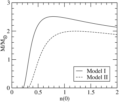
Figure 1: Mass $M$ (in units of solar mass $M_{\odot}$) vs the central neutron number density $n(0)$ (in units of ${\rm fm}^{-3}$) for the mean field coupling values of Models I and II of Table 1.

Table 1: Parameters describing our choice of mean field and canonical superfluid neutron star models.  The two values for $c^{2}_{\sigma}$ and $c^{2}_{\omega}$ represent the two extremes given in G97 that have been determined from nuclear physics.  Note that the baryon mass is $m=4.7582~{}{\rm fm}^{-1}$.

Model I	Model II
$c_{\sigma}^{2}=12.684$	$c_{\sigma}^{2}=8.403$
$c_{\omega}^{2}=7.148$	$c_{\omega}^{2}=4.233$
$\nu(0)=-2.316408$	$\nu(0)=-2.288385$
$k_{n}(0)=2.8~{}{\rm fm}^{-1}$	$k_{n}(0)=3.25~{}{\rm fm}^{-1}$
$x_{p}(0)=0.101$	$x_{p}(0)=0.102$
$M=2.509~{}M_{\odot}$	$M=1.996~{}M_{\odot}$
$R=11.696~{}{\rm km}$	$R=9.432~{}{\rm km}$

In several earlier studies LM00 ; PCA02 ; ACL02 , a parameterized model for entrainment has been used that is based on the Newtonian calculations of Borumand et al. BJK96 .  The parameter, $\varepsilon_{mom}$, in this model can be shown to be related to our coefficient $\left.{\cal A}\right|_{0}$ via

$$\varepsilon_{mom}={\left.{\cal A}\right|_{0}p\over m-\left.{\cal A}\right|_{0}\left(n+p\right)}\ .$$ (132)

In the previous studies the “physical” range has been taken to be $0.04<\varepsilon_{mom}<0.2$.  But already with this formula we find that $\varepsilon_{mom}$ has a singularity whenever $m=\left.{\cal A}\right|_{0}(n+p)$.  And in Fig. 2 we see that indeed $\varepsilon_{mom}$ has a discontinuity in both curves (which are for Models I and II of Table 1).  This is perhaps the most significant short term result of this work, and hence taking $\varepsilon_{mom}$ to be a constant must be considered a non-viable option.

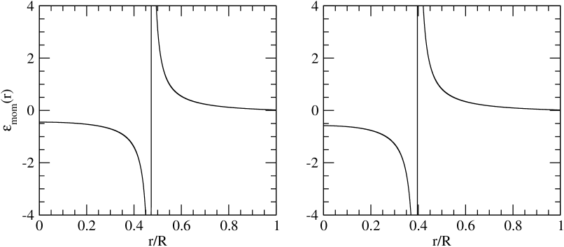
Figure 2: The entrainment parameter $\varepsilon_{mom}$ as a function of radius for Models I (left panel) and II (right panel) of Table 1.

An alternative parameterization is that of Prix et al. PCA02 . They point out that there is some ambiguity in what is meant by the nucleon effective masses (i.e. the Landau, as opposed to the Dirac, effective masses G97 ), which can be traced to whether one chooses to define these masses with respect to the zero-momentum or zero-velocity frame of the nucleons.  Their parameterization makes use of the zero-velocity frame.  In this case one finds

$$\varepsilon_{vel}={\left.{\cal A}\right|_{0}n\over m}\ .$$ (133)

Immediately we see that this formulation does not have an obvious singularity anywhere, and this is reflected in Fig. 3 which contains plots of the radial profile of $\varepsilon_{vel}$ for Models I and II of Table 1.  The “physical” range has been taken to be $0.4<\varepsilon_{vel}<0.7$.  We see from the figure that this is the range in the outer portion of the star, but in the core the entrainment stretches well out of this range.

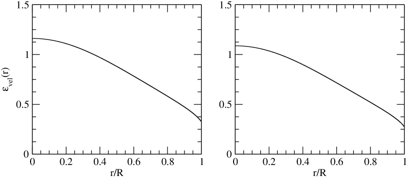
Figure 3: The entrainment parameter $\varepsilon_{vel}$ as a function of radius for Models I (left panel) and II (right panel) of Table 1.

Also used in Prix et al. PCA02 is the so-called symmetry energy parameter

$$\sigma={\partial\mu/\partial p\over\partial\chi/\partial n}$$ (134)

that can be related to terms PAL88 in the equation of state that tend to force an equal number of protons and neutrons (as in most nuclei).  For the relativistic mean field model used here, it is not difficult to show that $\sigma=1$ (which is consistent with the range of values used by PCA02 ).

IV Slow Rotation Configurations: The Frame-Dragging

The key distinguishing feature of slowly rotating superfluid neutron stars is that the neutrons can rotate at rates different from that of the protons.  The slow-rotation approximation is valid when the angular velocities are small enough that the fractional changes in pressure, energy density, and gravitational field due to the rotation are all relatively small.  This translates into the inequalities (cf. H67 ; AC01c )

$$\Omega^{2}_{n}~{}{\rm or}~{}\Omega^{2}_{p}~{}{\rm or}~{}\Omega_{n}\Omega_{p}~{}<<~{}\left({c\over R}\right)^{2}{GM\over Rc^{2}}\ ,$$ (135)

where the speed of light $c$ and Newton’s constant $G$ have been restored, and $R$ and $M$ are the radius and mass, respectively, of the non-rotating configuration.  Since $GM/c^{2}R<1$, we also see that

$$\Omega_{n}R<<c\qquad{\rm and}\qquad\Omega_{p}R<<c\ ,$$ (136)

and thus the slow-rotation approximation ought to be useful for most astrophysical neutron stars.  In fact a comparison AC01c ; PCA02 of the above conditions to empirical estimates for the Kepler frequency (i.e. the rotation rate at which mass-shedding sets in at the equator) that can been obtained from calculations using realistic supranuclear equations of state reveals that even the fastest observed pulsars can be classified as slowly rotating.

The only quantities that contain terms linear in the angular velocities are the metric coefficient $\omega(r)$, that represents the dragging of inertial frames, and the fluid four-velocities.  All other effects due to rotation enter at the second-order in the angular velocities.  It is useful to define

$$\tilde{L}_{n}=\omega-\Omega_{n}\quad,\quad\tilde{L}_{p}=\omega-\Omega_{p}\ .$$ (137)

Up to an overall minus sign, these represent rotation frequencies as perceived by local zero-angular momentum observers.  The Einstein equation that determines the frame-dragging has been shown to be AC01c

$${1\over r^{4}}\left(r^{4}e^{-(\lambda+\nu)/2}\tilde{L}_{p}^{\prime}\right)^{\prime}-16\pi e^{(\lambda-\nu)/2}\left(\left.\Psi\right|_{0}-\left.\Lambda\right|_{0}\right)\tilde{L}_{p}=16\pi e^{(\lambda-\nu)/2}\left.\mu\right|_{0}n\left(\Omega_{n}-\Omega_{p}\right)\ .$$ (138)

It is of the same form as that obtained by Hartle H67 except for the non-zero source term on the right-hand-side.

Exterior to the star, there is vacuum, and so the solution for the frame-dragging is the same as that considered by Hartle H67 , i.e.

$$\omega(r)={2J\over r^{3}}\ .$$ (139)

Assuming that the frame-dragging is continuous at the surface of the star, then

$$J=-{8\pi\over 3}\int_{0}^{R}{\rm d}rr^{4}e^{(\lambda-\nu)/2}\left[\left.\mu\right|_{0}n\tilde{L}_{n}+\left.\chi\right|_{0}p\tilde{L}_{p}\right]\ ,$$ (140)

where $J$ is the total angular momentum.  Andersson and Comer AC01c have furthermore shown that the neutron total angular momentum is

$$J_{n}=-{8\pi\over 3}\int_{0}^{R}{\rm d}rr^{4}e^{(\lambda-\nu)/2}\left[\left.\mu\right|_{0}n\tilde{L}_{n}+\left.{\cal A}\right|_{0}np\left(\Omega_{n}-\Omega_{p}\right)\right]$$ (141)

and

$$J_{p}=-{8\pi\over 3}\int_{0}^{R}{\rm d}rr^{4}e^{(\lambda-\nu)/2}\left[\left.\chi\right|_{0}p\tilde{L}_{p}+\left.{\cal A}\right|_{0}np\left(\Omega_{p}-\Omega_{n}\right)\right]$$ (142)

for the proton total angular momentum, from which it follows that

$$J=J_{n}+J_{p}\ .$$ (143)

Any solution of Eq. (138) for the frame-dragging is to be such that the interior matches smoothly onto the known vacuum solution in Eq. (139).  This means that we must have, for instance,

$$\tilde{L}_{p}(R)=-\Omega_{p}+{2J\over R^{3}}\ .$$ (144)

We can easily see that $\tilde{L}_{p}$ and its derivative are smooth provided that we have

$$\tilde{L}_{p}(R)=-\Omega_{p}-{R\over 3}\left.{d\tilde{L}_{p}\over dr}\right|_{r=R}\ .$$ (145)

Having obtained a value for $\tilde{L}_{p}(0)$ that satisfies Eq. (145), an acceptable solution is in hand, and we can thus determine the angular momentum of the configuration from Eq. (144).

In Fig. 4 we have plots of the radial profile of the frame-dragging for Model I for a range of values of the ratio $\Omega_{n}/\Omega_{p}$.  For the values considered in the left panel we see that the frame-dragging is much like that of an ordinary one-fluid star, and is consistent with solutions obtained by Andersson and Comer AC01c .  For the negative ratios, we see that the frame-dragging is negative but increases monotonically towards zero.  This is the behaviour we should expect, since the bulk of the matter is simply rotating the opposite way.  There is some asymmetry between the negative and positive ratios, but that is due to the small number of protons that rotate oppositely to the neutrons when the ratio is negative.  In the right panel, we examine the solutions near to a ratio of zero.  The frame-dragging is no longer monotonic and actually becomes negative inside the star.  An explanation of this can be understood as follows: in the interior the protons carry most of the angular momentum and thus have the largest impact on the frame-dragging, but further away from the center, the much larger mass contained in the neutrons begins to dominate AC01c .

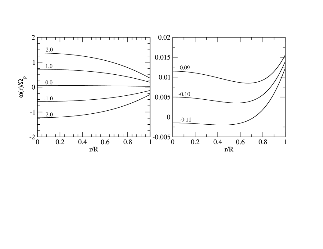
Figure 4: The radial profile of the frame-dragging $\omega(r)$ for Model I of Table 1.  In the left-panel we have curves for $\Omega_{n}/\Omega_{p}=(-2.0,-1.0,0.0,1.0,2.0)$, and in the right we have taken $\Omega_{n}/\Omega_{p}=(-0.11,-0.10,-0.09)$.

Fig. 5 considers the same range for the ratio of the angular speeds, by showing how the total angular momentum $J$, and the neutron and proton angular momenta, $J_{n}$ and $J_{p}$ respectively, vary as $\Omega_{n}/\Omega_{p}$ is changed.  As one might expect, when the ratio becomes greater than one, then the angular momentum in the neutrons is significantly greater than that of the protons.  Likewise, as the ratio becomes smaller we find that the protons can dominate.  Something of a surprise is the extreme right-hand-side of the curves, where $J_{p}$ actually becomes negative, and yet the angular speeds of the neutrons and protons have the same sign.  We can explain this behaviour as a purely general relativistic effect that is intimately connected with the frame-dragging.  With respect to infinity, particles that are rotating around at the same rate as the local inertial frames are found to have zero angular momentum.  Thus, those particles that would be lagging behind the frames, even though their angular trajectories would be in the same direction as the frames, will nevertheless have negative angular momentum.  Finally, one other feature is the configuration where $J_{n}=J_{p}$.  In this case, the angular speeds are not equal, nor are the total neutron and proton particle numbers equal, and yet the angular momenta of both fluids are the same.

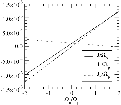
Figure 5: The neutron $J_{n}$, proton $J_{p}$, and total $J$ angular momenta vs the ratio $\Omega_{n}/\Omega_{p}$ for Model I of Table 1.

V Conclusions

We have developed a formalism that uses relativistic mean field theory for supra-nuclear density matter that can be applied to general relativistic superfluid neutron stars.  In this formalism we have also allowed for the entrainment effect between the various superfluid species.  We have also shown how to use our formalism in the relativistic superfluid field equations that have been recently developed for modelling slowly rotating equilbirium configurations AC01c , as well as the linearized oscillations CLL99 ; ACL02 .  Our results indicate that parameterized models of entrainment that use a zero-momentum rest-frame definition for nucleon effective masses have a singularity, whereas those based on zero-velocity rest-frames do not.

Our results should find a wide range of applications, not the least of which is to understand better the role of entrainment in the superfluid modes of oscillation (e.g. the avoided crossings described by AC01a ) and subsequent imprints AC01b ; GC02 that may be left in neutron star gravitational waves (emitted, for instance, during glitches).  Applications planned for the near future will include numerical studies of rapidly rotating superfluid neutron stars (using an adaptation of the very accurate LORENE code PNC02 ) and continued research on the newly discovered two-stream instability ACP02a ; ACP02b , which has been proposed as a trigger mechanism for glitches in pulsars.  For the rapid rotation calculations one must necessarily imploy the full formalism discussed here in the sense that $K$ will no longer be kept small, since the LORENE code is specifically designed to accurately handle relative velocities of the neutrons with respect to the protons that approach the speed of light.  And for the two-stream instability entrainment provides one of the main couplings between the two fluids.

Appendix: Limiting Forms

The slow-rotation approximation is such that only terms up to and including ${\cal O}(\Omega^{2}_{n,p})$ are required.  This translates into keeping only those terms in the mean field theory up to and including ${\cal O}(K^{2})$.  This is because those quantities like $m_{*}$ and $\Lambda$ are scalars, and can only depend on terms that are even in $K$.  Likewise, those quantities that are like vectors, e.g. $\omega_{z}$, can only depend on terms that are odd in $K$.  Because $m_{*}$ and $\omega_{z}$ are known only implicitly, we determine their expansion coefficients by assuming they take the form

$$\phi_{z} = \left.{\partial\phi_{z}\over\partial K}\right|_{0}K\ ,$$ (146)

$$m_{*} = \left.m_{*}\right|_{0}+\left.{\partial m_{*}\over\partial K^{2}}\right|_{0}K^{2}\ ,$$ (148)

where

$$\left.m_{*}\right|_{0} = m_{*}(k_{n},k_{p},0)$$ (149)

$$= m-\left.m_{*}\right|_{0}{c_{\sigma}^{2}\over 2\pi^{2}}\left(k_{n}\sqrt{k^{2}_{n}+\left.m^{2}_{*}\right|_{0}}+k_{p}\sqrt{k^{2}_{p}+\left.m^{2}_{*}\right|_{0}}+{1\over 2}\left.m_{*}^{2}\right|_{0}{\rm ln}\left[{-k_{n}+\sqrt{k^{2}_{n}+\left.m^{2}_{*}\right|_{0}}\over k_{n}+\sqrt{k^{2}_{n}+\left.m^{2}_{*}\right|_{0}}}\right]+\right.$$ (153)

$${1\over 2}\left.\left.m_{*}^{2}\right|_{0}{\rm ln}\left[{-k_{p}+\sqrt{k^{2}_{p}+\left.m^{2}_{*}\right|_{0}}\over k_{p}+\sqrt{k^{2}_{p}+\left.m^{2}_{*}\right|_{0}}}\right]\right)\ .$$

By inserting Eq. (148) into Eq. (92), and expanding and keeping terms to the appropriate orders, we find

$$\left.{\partial\phi_{z}\over\partial K}\right|_{0} = -{c_{\omega}^{2}\over 3\pi^{2}}{k^{3}_{p}\over\sqrt{k^{2}_{p}+\left.m^{2}_{*}\right|_{0}}}\left(1+{c_{\omega}^{2}\over 3\pi^{2}}\left[{k^{3}_{n}\over\sqrt{k^{2}_{n}+\left.m^{2}_{*}\right|_{0}}}+{k^{3}_{p}\over\sqrt{k^{2}_{p}+\left.m^{2}_{*}\right|_{0}}}\right]\right)^{-1}\ ,$$ (154)

$$\left.{\partial m_{*}\over\partial k_{n}}\right|_{0} = -{c_{\sigma}^{2}\over\pi^{2}}{\left.m_{*}\right|_{0}k^{2}_{n}\over\sqrt{k^{2}_{n}+\left.m^{2}_{*}\right|_{0}}}\left({3m-2\left.m_{*}\right|_{0}\over\left.m_{*}\right|_{0}}-{c_{\sigma}^{2}\over\pi^{2}}\left[{k^{3}_{n}\over\sqrt{k^{2}_{n}+\left.m^{2}_{*}\right|_{0}}}+{k^{3}_{p}\over\sqrt{k^{2}_{p}+\left.m^{2}_{*}\right|_{0}}}\right]\right)^{-1}\ ,$$ (156)

$$\left.{\partial m_{*}\over\partial k_{p}}\right|_{0} = -{c_{\sigma}^{2}\over\pi^{2}}{\left.m_{*}\right|_{0}k^{2}_{p}\over\sqrt{k^{2}_{p}+\left.m^{2}_{*}\right|_{0}}}\left({3m-2\left.m_{*}\right|_{0}\over\left.m_{*}\right|_{0}}-{c_{\sigma}^{2}\over\pi^{2}}\left[{k^{3}_{n}\over\sqrt{k^{2}_{n}+\left.m^{2}_{*}\right|_{0}}}+{k^{3}_{p}\over\sqrt{k^{2}_{p}+\left.m^{2}_{*}\right|_{0}}}\right]\right)^{-1}\ ,$$ (158)

$$n^{z} = {1\over 3\pi^{2}}{k^{3}_{n}\over\sqrt{k^{2}_{n}+\left.m^{2}_{*}\right|_{0}}}\left.{\partial\phi_{z}\over\partial K}\right|_{0}K\ ,$$ (160)

$$p^{z} = {1\over 3\pi^{2}}{k^{3}_{p}\over\sqrt{k^{2}_{p}+\left.m^{2}_{*}\right|_{0}}}\left(\left.{\partial\phi_{z}\over\partial K}\right|_{0}+1\right)K\ .$$ (162)

We note that the coefficient $\left.\partial m_{*}/\partial K^{2}\right|_{0}$ cancels everywhere, which is why it is not written here.  Also, we find

$$\left.\Lambda\right|_{0} = -{1\over 4\pi^{2}}\left(k_{n}^{3}\sqrt{k^{2}_{n}+\left.m^{2}_{*}\right|_{0}}+k_{p}^{3}\sqrt{k^{2}_{p}+\left.m^{2}_{*}\right|_{0}}\right)-{1\over 2}m^{2}_{\omega}\omega_{0}^{2}-{1\over 4}c_{\sigma}^{-2}\left(2m-\left.m_{*}\right|_{0}\right)\left(m-\left.m_{*}\right|_{0}\right)-$$ (165)

$${1\over 8\pi^{2}}\left(m_{e}k_{p}\left[2k_{p}+m_{e}\right]\sqrt{k_{p}^{2}+m^{2}_{e}}-m^{4}_{e}{\rm ln}\left[{k_{p}+\sqrt{k^{2}_{p}+m^{2}_{e}}\over m_{e}}\right]\right)\ ,$$

$$\left.\mu\right|_{0} = g_{\omega}\omega_{0}+\sqrt{k^{2}_{n}+\left.m^{2}_{*}\right|_{0}}\ ,$$ (167)

$$\left.\chi\right|_{0} = g_{\omega}\omega_{0}+\sqrt{k^{2}_{p}+\left.m^{2}_{*}\right|_{0}}\ ,$$ (169)

$$\left.\Psi\right|_{0} = \left.\Lambda\right|_{0}+{1\over 3\pi^{2}}\left(\left.\mu\right|_{0}k_{n}^{3}+\left[\left.\chi\right|_{0}+\sqrt{k_{p}^{2}+m^{2}_{e}}\right]k_{p}^{3}\right)\ .$$ (171)

The condition of chemical equilibrium is that $\left.\mu\right|_{0}=\left.\chi\right|_{0}+\sqrt{k^{2}_{p}+m^{2}_{e}}$.

References

• (1) N. Andersson and G. L. Comer, Class. and Quant. Grav. 18, 969 (2001).
• (2) N. Andersson and G. L. Comer, Phys. Rev. Lett. 24, 241101 (2001).
• (3) G. L. Comer, Found. of Phys., in press (2002); also available as LANL preprint archive astro-ph/0207608.
• (4) N. Andersson, G. L. Comer, and D. Langlois, Phys. Rev. D 66, 104002 (2002); also available as preprint LANL archive gr-qc/0203039.
• (5) N. Andersson and G. L. Comer, Mon. Not. R. Astron. Soc. 328, 1129 (2001).
• (6) R. Prix, G. L. Comer, and N. Andersson, Astron. Astrophys. 381, 178 (2002).
• (7) N. Andersson, G. L. Comer, and R. Prix, submitted to Phys. Rev. Letts. (2002); also available as LANL preprint archive astro-ph/0210486.
• (8) N. Andersson, G. L. Comer, and R. Prix, Mon. Not. R. Astron. Soc., to appear(2003); also available as LANL preprint archive astro-ph/0211151.
• (9) J. Sauls, in Timing Neutron Stars, eds. H. Ögelman and E. P. J. van den Heuvel, (Dordrecht, Kluwer, 1989), pp. 457-490.
• (10) L. Lindblom and G. Mendell, Phys. Rev. D 61, 104003 (2000).
• (11) M. Borumand, R. Joynt, and W. Klúzniak, Phys. Rev. C 54, 2745 (1996).
• (12) C. W. Misner, K. Thorne, and J. A. Wheeler, Gravitation (Freeman, San Francisco, 1973).
• (13) N. K. Glenndenning, Compact Stars: Nuclear Physics, Particle Physics, and General Relativity, (Springer-Verlag, New York, 1997).
• (14) S. A. Chin and G. Baym, Nucl. Phys. A 262, 527 (1976).
• (15) B. Carter, “Relativistic fluid dynamics”, A. Anile and M. Choquet-Bruhat, Eds., Springer-Verlag (1989).
• (16) G. L. Comer and D. Langlois, Class. and Quant. Grav. 11, 709 (1994).
• (17) B. Carter and D. Langlois, Phys. Rev. D 51, 5855 (1995).
• (18) B. Carter and D. Langlois, Nucl. Phys. B 454, 402 (1998).
• (19) B. Carter and D. Langlois, Nucl. Phys. B 531, 478 (1998).
• (20) D. Langlois, A. Sedrakian, and B. Carter, Mon. Not. R. Astron. Soc. 297, 1189 (1998).
• (21) G. L. Comer, D. Langlois, and L. M. Lin, Phys. Rev. D 60, 104025 (1999).
• (22) R. Prix, Phys. Rev. D 62, 103005 (2000).
• (23) R. I. Epstein, Ap. J. 333, 880 (1988).
• (24) R. Prix, J. Novak, and G. L. Comer, LANL preprint archive gr-qc/0211105.
• (25) S. L. Shapiro and S. A. Teukolsky, Black Holes, White Dwarfs and Neutron Stars. The Physics of Compact Objects, (Wiley, New York, 1983).
• (26) M. Prakash, T. L. Ainsworth, and J. M. Lattimer, Phys. Rev. Lett. 61, 2518 (1988).
• (27) J. B. Hartle, Ap. J. 150, 1005 (1967).