The Causal Set approach to quantum gravity asserts that spacetime, at its smallest length scale, has a discrete structure. This discrete structure takes the form of a locally finite order relation, where the order, corresponding with the macroscopic notion of spacetime causality, is taken to be a fundamental aspect of nature.

After an introduction to the Causal Set approach, this thesis considers a simple toy dynamics for causal sets. Numerical simulations of the model provide evidence for the existence of a continuum limit. While studying this toy dynamics, a picture arises of how the dynamics can be generalized in such a way that the theory could hope to produce more physically realistic causal sets. By thinking in terms of a stochastic growth process, and positing some fundamental principles, we are led almost uniquely to a family of dynamical laws (stochastic processes) parameterized by a countable sequence of coupling constants. This result is quite promising in that we now know how to speak of dynamics for a theory with discrete time. In addition, these dynamics can be expressed in terms of state models of Ising spins living on the relations of the causal set, which indicates how non-gravitational matter may arise from the theory without having to be built in at the fundamental level.

These results are encouraging in that there exists a natural way to transform this classical theory, which is expressed in terms of a probability measure, to a quantum theory, expressed in terms of a quantum measure. A sketch as to how one might proceed in doing this is provided. Thus there is good reason to expect that Causal Sets are close to providing a background independent theory of quantum gravity.

Acknowledgements

I would like to express deep gratitude for my advisor, Rafael Sorkin, for his patient teaching and support throughout my graduate career. His depth of insight into fundamental issues in physics is extremely helpful and illuminating. I also would like to thank Peter Saulson, for acting as my advisor at a critical stage in my graduate career, providing much needed support and encouragement. Let me also express my appreciation to Fatma Husein for some very illuminating conversations, Scott Klasky for teaching me how to write efficient code, Asif Qamar for introducing me to GNU/Linux at a critical time, and Saul Teukolsky for kind hospitality at Cornell. Thank you to my fellow students who helped me in many ways throughout my time at Syracuse — Bill Kahl, Eric Gregory, Asif Qamar, Rob Salgado, Arshad Momen, Jim Javor, and many others.

In addition, let me thank Lawrence Lyon and Nelson Mead, for standing with me in prayer, and especially Lawrence for many discussions both about the physics and the larger perspective of life. Let me also thank Wayne Lytle, for teaching me about C++, and the rest of the people of Covenant Love Community Church/School, especially Kathy Mead, for their support in prayer, meals, babysitting, raw labor, and more, while I was finishing this work.

Finally, I would like to thank my family, for their endless patience, and especially my wife, Yvonne Tempel, for her love, exemplary patience, continuous pressure, and reminders of a broader perspective. My daughter Kendra deserves special thanks for her encouraging hugs.

This is dedicated to the memory of my father, Donald C. Rideout, whose support in the beginning made all of this possible.

Chapter 1 Introduction to Causal Sets

1.1 Quantum gravity in general

The quest for a theory of quantum gravity arises from the fundamental inconsistencies of quantum mechanics and general relativity. Due to the philosophical differences between the two theories, it appears that a successful marriage of the two will occur only with a radical reformulation of both theories. In thinking about how to approach such a reformulation, one must decide which aspects of nature are fundamental, and which arise as “emergent” structures [57].

There are strong indications that nature, at its smallest length scale, has a discrete structure. The ultraviolet divergences of quantum field theory and the singularities of general relativity are two examples. The infinite “entanglement entropy” of a black hole in semi-classical gravity is another indication. (In fact, a continuum is not experimentally verifiable by any finite experiment, even in principle.)

In the case of causal sets, two aspects are regarded as fundamental — discreteness and causality. The choice of causality as a fundamental notion is partly aesthetic, and partly due to the great success one has in recovering other aspects of spacetime geometry from a causal order. The Causal Set program postulates that spacetime is a macroscopic approximation to an underlying discrete causal order. The other familiar properties of a spacetime manifold, such as its metrical geometry and Lorentzian signature, arise as “emergent” properties of the underlying discrete order.

Mituo Taketani, a Japanese physicist and philosopher of science, has described the process of physical theory construction in terms of three distinct stages [63]. The three stages repeat cyclically, except after each cycle the theory is understood at a deeper level. The three stages, using physics terminology, may be called the phenomenological, kinematical, and dynamical.

The phenomenological stage concerns itself with what physical phenomena the theory seeks to address. For what observational results should the theory provide explanation? For the Copernican model of the solar system, an example of the phenomena would be the retrograde motion of the planets with respect to the fixed background stars.

In the kinematical stage one decides in what language the theory will be expressed. What are the basic elements of the theory, the “substance”, and how do they interrelate? For the case of general relativity, one chooses a manifold with a Lorentzian metric. This stage is very important, as in it one decides “what really exists” in nature. It determines the mathematical and philosophical construct on which the theory will be based.

Once a language is set in place, and the basic constructs of the theory are chosen, then the remaining task is to determine how these objects behave. What are the “equations of motion” of the theory? In the case of General Relativity, this would be the Einstein equations. It selects which of the kinematical possibilities (in this example spacetime manifolds) will be realized by nature. After finishing the third stage, then one will observe new phenomena which are still not explained by the theory, which then begins the phenomenological stage of the next cycle. Each successive theory will contain those of the earlier cycles, generally as some limiting form of the latest theory.

This thesis presents a step towards understanding the full quantum dynamics of spacetime.

Prior to this work, most knowledge about causal sets was kinematical in nature. This involved questions such as when a causal set is well approximated by a continuum spacetime, and what characteristics of a causal set one can “measure” to extract information about the spacetime into which it might faithfully embed. However, little was understood about the dynamics of causal sets. One of the primary difficulties was that most of our experience with dynamics was for continuum theories, where one can easily write down Lagrangians with differential operators. Causal sets unfortunately seemed to repel attempts to construct an action using simple analogy with existing continuum theories. An entirely new approach was needed to express the dynamics of the theory.

There exist other discrete approaches to quantum gravity which involve a causal ordering. Some examples are discussed in [28, 4, 37].

1.2 Kinematics of Causal Sets

In the case of Causal Sets, the causal set is the kinematical “substance” of the theory. The kinematical stage of causal sets then concerns itself with understanding how the spacetime manifold emerges from the underlying discrete causal order.

Note that a causal structure is a natural choice for the “substance” of the theory, because it encodes all the information of a continuum spacetime (metrical geometry, topology, differential structure) save a conformal factor. Thus all that is missing is the volume information. However, since the theory is discrete, this arises naturally as well, from counting. So a discrete causal structure has sufficient information to encode all the kinematical framework of general relativity.

1.2.1 Mathematical Definitions

A partially ordered set, or poset, is a set $S$ with order relation $\prec$ which is irreflexive ($x\not\prec x\;\;\forall x\in S$) and transitive ($x\prec y$ and $y\prec z\Rightarrow x\prec z\;\;\forall x,y,z\in S$). An (induced) subposet of a poset $P$ is a subset $P^{\prime}\subset P$ whose order relation is determined by the condition that $x\prec y$ in $P^{\prime}$ iff $x\prec y$ in $P$. An interval (sometimes called an Alexandrov set or Alexandrov region) $\mathrm{int}[x,y]$ in a poset $P$ is the induced subposet $P^{\prime}$ defined by the set of all elements $\{z|x\prec z\prec y\}$. A causal set is defined to be a partial order for which every interval $\mathrm{int}[x,y]\;\forall x,y$ has finite cardinality. An order which obeys this condition on the cardinality of all intervals is called locally finite.

In a causal set $(S,\prec)$, a pair of elements $x,y\in S$ such that $x\prec y$ form a relation; one writes that $x$ and $y$ are related, that $x$ precedes $y$, $y$ succeeds $x$ ($y\succ x$), $x$ is an ancestor of $y$, and $y$ is a descendent or successor of $x$. The past of an element $x\in{S}$ is the subset $\mathrm{past}(x)=\{y\in{S}\,|\,y\prec{x}\}$, i.e. the set of all ancestors of $x$. The past of a subset of $S$ is the union of the pasts of its elements. The future of an element, $\mathrm{future}(x)$, is the set of all descendents of $x$. A link is a relation for which there is no $z$ such that $x\prec z\prec y$. A link is an irreducible relation, that is, one not implied by other relations via transitivity.

A Hasse diagram is a pictorial representation of a poset. In the diagram, each element of the poset is represented as a dot. A line connects any two elements $x\prec y$ related by a link, such that the preceding element $x$ is drawn below the succeeding element $y$ (as is the case in spacetime diagrams).

A chain, or total order, is a set of elements for which each pair is related by $\prec$. An $n$-chain is a chain with $n$ elements. A path in a poset is an increasing sequence of elements, each related to the next by a link, i.e. it is a “chain made of links”. More precisely, a path $C$ between two elements $x\prec y$ is a chain which has $x$ as its past endpoint and $y$ as its future endpoint, for which there exists no element $z$ comparable with all elements in $C$ such that $x\prec z\prec y$. The length of a path is its number of elements. An antichain is a set of elements in which no pair are related by $\prec$. Note that this corresponds to an “achronal” or “acausal” set in spacetime. An $n$-antichain is an antichain with $n$ elements. A maximal antichain $A$ is an inextendible antichain, i.e. there does not exist any element of the poset which is unrelated to every element of $A$. A maximal antichain would correspond roughly to an “edgeless achronal set”, or Cauchy surface assuming global hyperbolicity. The height of an order is the length of the longest chain in that order (or, equivalently, the length of the longest path), while the width is the size of the largest antichain. An $N$-order is a partial order defined on $N$ elements. A covering graph of an order is the order’s Hasse diagram, regarded as an undirected graph. A connected component of an order is subset of elements which form a connected (sub)graph in the covering graph of the order. i.e. it is a subposet for which any two points are connected by a set of paths. A maximal element is one which has no successors, i.e. an element $x$ for which $\not\hskip-2.0pt\exists\,y\in S\,|\,x\prec y$. A minimal element is one which has no ancestors, i.e. an element $x$ for which $\not\hskip-2.0pt\exists\,y\in S\,|\,y\prec x$. An automorphism is a one-to-one map of $S$ onto itself that preserves $\prec$.

1.2.2 Faithful Embedding — Correspondence with the Continuum

Consider a (Hausdorff, paracompact) manifold $M$ with a globally hyperbolic, time orientable, Lorentzian, smooth metric $g_{ab}$. Consider a map $\phi:S\rightarrow M$ from a causal set $C=(S,\prec)$ into a spacetime $(M,g_{ab})$. We call this map a conformal embedding if $x\prec y\Leftrightarrow f(x)\in J^{-}(f(y))\;\;\forall x,y\in S$. Consider an Alexandrov region of $(M,g_{ab})$, $J^{+}(p)\cap J^{-}(q)$ for every $p,q\in M$. The map $\phi$ is called a faithful embedding if it has two further properties. Firstly, the number of points $n$ mapped into an Alexandrov region is equal to its spacetime volume $V$, up to Poisson fluctuations, i.e. the probability of getting $n$ points in the region is

$$P(n)=\frac{(\rho V)^{n}e^{-\rho V}}{n!}\,,$$

where $\rho$ is the density set by the fundamental length scale. Second, the mean spacing between points in the embedding, $\rho^{-1/d}$ in $d$ dimensions, must be everywhere much less than the characteristic length scale $\lambda$ over which the continuum geometry varies. (Admittedly these properties are not entirely well defined yet, but they provide a good heuristic notion.) We say that a spacetime $M$ approximates a causal set $C$ if there exists a faithful embedding of $C$ into $M$. See [14] for more discussion on this issue.

The notion of faithful embedding gives a correspondence between a causal set and a continuum spacetime. The belief is that a given causal set embeds faithfully into a unique spacetime. Expressed more precisely, if $\phi:C\rightarrow M$ and $\phi^{\prime}:C\rightarrow M^{\prime}$ are two faithful embeddings into two spacetimes $M$ and $M^{\prime}$, then there exists an approximate isometry $g:M\rightarrow M^{\prime}$ such that $\phi^{\prime}=g\circ\phi$. The isometry will only be approximate because the condition of faithful embedding is not sufficient to fix the entire continuum geometry — there will remain small variations in the geometry, with length scale $>\lambda$, which still admit a faithful embedding of $C$. In general the precise formulation and proof of this conjecture, which is called the “Hauptvermutung” of Causal Sets, is a difficult mathematical problem.

Given an arbitrary (past and future distinguishing) spacetime, it is easy to construct a causal set which will admit a faithful embedding into that spacetime. The method, suggestively called sprinkling, is to simply select at random, via a Poisson distribution, a finite set of events of the spacetime. These will correspond to the elements of the causal set. The causal relations of the causal set are simply those inherited directly from spacetime causality.

Note that in a faithfully embedded causal set most links will then be “almost null”, due to the Lorentz invariance of (local) spacetime. There can exist two events which are spatially very distant, perhaps lying in different galactic clusters, which are nevertheless “nearest neighbors” in the sense that they are connected by an (almost) null geodesic. (Also note in this connection that causal sets naturally suggest a sort of “blurring” between the ultraviolet and the infrared, in that a field that is highly boosted gets blueshifted, while at the same time it makes connection with remote parts of the universe. The extent to which a field can be boosted (ultraviolet cutoff) is limited by the size of the universe (infrared cutoff), as increasing large boosts require the existence of links connecting increasingly “distant” elements of the causal set.)

So the causal set is a “discrete manifold”, using the words of Riemann, from which the macroscopic properties of the continuum spacetime: topology, differential structure, metrical geometry, and causal structure, are emergent. Note that by keeping the causal structure as the substance of the theory, and then “counting” to get volume information, we have been able to recover the full metrical geometry. This succeeds because the causal structure of a spacetime completely determines its metric up to a conformal factor [36]. The discreteness, “number”, by providing the missing volume information, restores the full metrical geometry. Note also that topology is restored, by inheritance from the topology of the manifold into which the causal set will faithfully embed. Note that the Lorentzian signature also arises naturally from this scheme, as the unique signature which maintains the distinctness of past and future directions in the causal order.

A considerable amount of work has been done in understanding the kinematics of causal sets. For example it is understood how to extract spacetime dimension and proper time from only the discrete causal order. The dynamics, however, was much less developed before this work. Below is a brief sketch of some of these earlier results.

1.2.3 Causal Set Dimension

There are many different indicators of the dimension of a causal set, that is, ways to estimate the dimension $d$ of the spacetime into which a given causal set might faithfully embed. The actual value of this dimension is the physical dimension. To determine directly the physical dimension of a causal set one would need a faithful embedding, which is difficult to achieve. The hope, then, is to deduce what this dimension will be by looking at certain simpler indicators which depend only on more easily accessible features of the causal order.

1.2.3.1 Integral dimension indicators

The following dimension indicators use only “conformal information” of the causal set, i.e. they only consider conformal embeddings in their construction, rather than faithful embeddings.

Linear dimension

Linear dimension (also called combinatorial dimension) is a definition of dimension for a poset generally used by mathematicians. It is not quite appropriate for causal sets, however, as the “light cones” it uses to define the order are “square” and thus will not be a good dimension indicator for embeddings into Minkowski space. It is defined as the minimum dimension $d$ such that the poset $P$ can be realized as points in $\hbox{\openface R}^{n}$ with the order given by $x\prec y\Leftrightarrow x_{i}<y_{i}\;\;\forall i$. In spite of its unphysical character, there are many results known for this notion of dimension.

Flat conformal embedding dimension

The flat conformal embedding dimension (also called Minkowski dimension, or causal dimension) is the minimum dimension Minkowski space into which the causal set can be causally embedded. Since in general one would expect the causet to embed into Minkowski space only locally (spacetime is locally flat), the more appropriate question to ask is that an (appropriately chosen) sub-causal set embed into Minkowski space, where the subcauset is chosen such that it is “small enough” to “not see the curvature” of the larger spacetime. These subsets, then, should contain the dimensionality information of the causet. Some conjectural bounds have been placed on causal dimension, in part by using results known for linear dimension. Some pixies can be identified, which, if present as subposets, establish a lower bound on flat conformal embedding dimension. See [14] and [20].

There are a number of difficulties with the notion of causal dimension. One is the problem of deciding how to choose a “local” subset which may represent a “small” region of the spacetime. For causal sets locality is very difficult to define, because the “unit balls” of the Lorentzian metric contain spatially very distant points. There are indications that a notion of locality is maintained in causal sets [23, 52], but it remains difficult to see how to use this to construct local subsets. Another shortcoming is that it is not unreasonable to imagine that the dimensionality of spacetime will vary with length scale. Thus the dimensional information encoded in one of these subsets should have length scale dependence. If the appropriate subset can be chosen only after some probabilistic process of coarse graining (see Section 1.2.6), the arguments used to establish bounds on flat conformal embedding dimension will no longer be valid. Lastly, as alluded to in an earlier footnote, it may be too strict to demand an exact conformal embedding. Then, for example, one cannot use pixies to establish firm bounds on dimension.

These difficulties illustrate how in general it is difficult to construct a global, exact indicator of dimension. The more useful notions are quasilocal, probabilistic, and fractal in nature, taking advantage of the volume information of a faithful embedding.

1.2.3.2 Fractal dimension indicators

There are other indicators of causal set dimension which depend on the volume information as well, i.e. they consider faithful embeddings in their definition. Consider an Alexandrov region $\mathrm{int}(x,y)$ of a causal set $C$. One can derive causal set invariants by counting the occurrence of various substructures, such as the number of relations, number of elements, number of chains, number of links, etc., and compare the result with what is known for sprinklings into $n$-dimensional Minkowski space, obtaining a dimension estimate for (that region of) the causal set from which the region was taken. Since the number (of relations, say) counted will never come out exactly as that which would arise from sprinkling into an integral dimension Minkowski space, the dimension which obtains from this procedure will always be fractional, as in computing the effective dimension of fractals.

This fractal dimension will be most meaningful if there exists a large region of $C$ covered by many Alexandrov sets of (approximately) the same cardinality $V$, which all yield (approximately) the same effective dimension $n_{\mathrm{eff}}$. In general different pairs of points $(x,y)$ will not yield the same $n_{\mathrm{eff}}$. This will occur for a number of reasons:

• random fluctuations.

• sampling a different region of the causal set.

• curvature of causet/spacetime: Because the region of spacetime enclosed within the interval $\mathrm{int}(x,y)$ in general will not be flat, the relationship between number of relations, say, and dimension will not quite be the same as that for flat spacetime. For this reason it is important to choose intervals which are much smaller than the curvature scale.

• scale dependence of topology, though this would vanish if we constrain $V$ to be same in each region $\mathrm{int}(x,y)$.

In addition, it should be noted that the notion of “covering a region of $C$ with many Alexandrov sets” may be relying on an intuition which is not valid for causal sets. The important point is that in any given reference frame, almost all Alexandrov sets “look extremely null”. Thus it is difficult to “tile” a region with such sets, a task which looks something like trying to cover a two dimensional region with a collection of thickened diagonal lines. In general each Alexandrov set will overlap a very large number of “neighboring tiles”, and will not cover the region in the same manner as one’s intuition from Riemannian signature geometries suggests.

Volume – length scaling

In $d$-dimensional Minkowski space, an Alexandrov set of “height” $T$ (proper time between its two end points) has spacetime volume

$$V=\frac{2V_{d-1}}{d}\left(\frac{T}{2}\right)^{d}=\frac{2\pi^{(d-1)/2}}{((d-1)/2)!\>d}\left(\frac{T}{2}\right)^{d}$$ (1.1)

where $V_{d}$ is the volume of a unit $d$-ball. For a given Alexandrov set $A=\mathrm{int}[x,y]$, measure $T$ by finding the longest chain connecting $x$ and $y$ (see sec. 1.2.4.1 below), count the number of elements $z$ in $A$, and invert (1.1) to get a dimension. This is perhaps the most obvious measure of dimension — to simply determine the exponent with which the volume of a region scales with length.

A caveat about this scheme is the unknown coefficient $m_{d}$ relating length of the longest chain to proper time (1.3).

Counting chains

Consider an interval $\mathrm{int}[a,b]$ which contains $N$ points and $C$ chains. Then in the limit of large $N$,

$$d=\frac{\ln N}{\ln\ln C}$$ (1.2)

is a measure of the causal set’s dimension. This measure is useful because it can be written explicitly, but is perhaps impractical because of the $\ln\ln$ in the denominator. ((1.2) follows from the fact that the number of chains $C$ in an interval grows exponentially with its height $T$, while its volume ($N$) grows as $T^{d}$ in $d$ dimensions.)

Myrheim-Meyer dimension

For a causal set $(S,\prec)$ define $R$ to be the number of related pairs of elements, i.e. the number of pairs $(x,y)$ such that $x\prec y$ or $y\prec x\;\>\forall x,y\in S$, and (following Myrheim [41]) define the ordering fraction $r$ to be the fraction of pairs of elements which are related, i.e. $r=R/{N\choose 2}$. A causal set which is formed by sprinkling $N$ points into an interval of $d$ dimensional Minkowski space will have an ordering fraction given by

$$r=\frac{3}{2}\frac{d!(d/2)!}{(3d/2)!}\,,$$

which decreases monotonically with dimension [40]. Inverting this relationship (numerically) yields a fractal dimension for any given $r$, called the Myrheim-Meyer dimension. Since this measure is based on measuring a large number ($R$), the random fluctuations will be smaller than those arising from similar dimension estimators which count other quantities, making this a computationally efficient method to estimate causal set dimension.

Because this measure of dimension associates a dimension to any ordering fraction $r$, it is sometimes used heuristically to specify the “dimension” of a causal set as a whole, without regard to whether it represents an Alexandrov set or whether the region is small enough not to see the spacetime curvature.

Midpoint scaling dimension

Consider an Alexandrov set $\mathrm{int}[x,y]$ of volume $V$. A midpoint, $z$, between $x$ and $y$, will subdivide $\mathrm{int}[x,y]$ into 3 regions $\mathrm{int}[x,z]$, $\mathrm{int}[z,y]$, and the remainder. If this causet is faithfully embeddable into $\openface{M}$, then the volume $V_{R}$ of the first two of these regions will be $(1/2)^{d}V$. Inverting this gives a dimension estimate of $d=\log_{2}(V/V_{R})$. A convenient definition for the midpoint is to maximize the minimum of $V(x,z)$ and $V(z,y)$.

1.2.4 Geometry

The previous section discussed briefly how to extract some topological information from the discrete order. Here I mention some ideas on how to extract geometrical information.

1.2.4.1 Proper time

The causal set should tell us not only whether two events are related, but “how much to the future” one occurred after the other.

Consider two elements in a causal set $x\prec y$. The longest chain connecting them will be a path, which may be called a (timelike) geodesic. Note that this corresponds directly to the notion of timelike geodesic in continuum spacetime — it is an extremal chronological curve connecting $x$ and $y$. For a causal set which embeds faithfully into a spacetime, there will usually be an extremely short path between any two related elements, e.g. one composed of two links, because one can always go as far out along the light cone as one wishes (“following a link”) and likely find an element which is linked to $x$. Recall, however, that for Lorentzian geometry the appropriate (timelike) extremal path is the longest path. Note that in general there may be multiple longest chains passing through two elements. In this sense the discrete notion of geodesic departs from the continuum (in a small region), but still a unique path length is assigned to the pair $x$ and $y$. In fact, this path length is proportional to the proper time interval of Minkowski spacetime, in the following sense.

Consider a causal set which arises from sprinkling into $d$-dimensional Minkowski space. Brightwell and Bollobás [9, 18] have shown that for an interval $\mathrm{int}[x,y]$ of volume $\rho V$, the length $L$ of the longest chain satisfies $L(\rho V)^{-1/d}\rightarrow m_{d}$ in probability, where $m_{d}$ is an unknown constant which depends on the dimension of the Minkowski space. Fairly tight bounds can be placed on $m_{d}$. For $d\geq 3$

$$1.77\leq\frac{2^{1-1/d}}{\Gamma(1+1/d)}\leq m_{d}\leq\frac{2^{1-1/d}e\Gamma(d+1)^{1/d}}{d}\leq 2.62$$ (1.3)

and it is known that $m_{2}=2$. Assuming that this correspondence remains in the presence of curvature, this provides a simple explicit method to extract timelike distances from the discrete order. For simplicity, we define proper time between two related elements to be the length of the longest chain connecting them.

Quite a bit is known about the fluctuations in this length as well, see e.g. [10]. Owing to the fact that a sprinkling into an interval of $\openface{M}^{2}$ is isomorphic to a random permutation, and that the length of the longest increasing subsequence (which is equivalent to the length of the longest chain) has been studied extensively, much is known about the 2 dimensional case [6, 5].

1.2.4.2 Spacelike distance

It is difficult to construct a notion of spacelike distance on a causal set, in part because of the non-compactness of the Lorentz group. For example, an early proposal by ’t Hooft [62] went essentially as follows, for $\openface{M}$. For two unrelated elements $(x,y)$, find the pair of elements $(a,b)$, such that $a\prec x,\>a\prec y,\>b\succ x$, and $b\succ y$, which minimizes the proper time (as computed in the previous section) between $a$ and $b$. Unfortunately this will always turn out to be zero (for sprinklings of $\openface{M}$ for $d>2$), because there will always be a pair $(a,b)$ which, by a statistical fluctuation, are linked. To see this, consider in $\openface{M}$ every pair $(a,b)$ where $a$ is chosen from the intersection of the past light cones of $x$ and $y$ (this is where the maximal elements of $\mathrm{past}(x)\cap\mathrm{past}(y)$ will lie) and $b$ is chosen from intersection of the future light cones of $x$ and $y$. Since these regions are noncompact, there will be an infinite number of (approximately) statistically independent pairs to consider, leading to certainty of finding a linked pair.

However, there is a proposal for finding the spacelike distance between a maximal chain and a point [18]. The construction is simply this: for a geodesic $\gamma$ and a point $x$ (the construction assumes that $\gamma$ is chosen such that $\mathrm{future}(x)\cap\gamma\neq\emptyset$ and $\mathrm{past}(x)\cap\gamma\neq\emptyset$) find the minimal point $b$ in $\mathrm{future}(x)\cap\gamma$ and the maximal point $a$ in $\mathrm{past}(x)\cap\gamma$, and take the spacelike separation between $\gamma$ and $x$ to be half the timelike distance between $a$ and $b$ (i.e. half the number of links in $\gamma$ between $a$ and $b$.

1.2.4.3 Curvature

One way to extract curvature information from the causal set is generalize Equation (1.1), as done in [41], to the case of non-zero curvature. From this one can extract information about the Ricci tensor [14]. The smaller intervals could be used to measure dimension, and then larger ones could be used to estimate curvature.

1.2.5 Closed Timelike Curves

The irreflexivity of the definition of a partial order used here is simply a convenient convention. One could just as well have chosen to define the poset to be reflexive ($x\prec x\;\>\forall x\in S$), but then an added condition of acyclicity would be required: $x\prec y$ and $x\neq y\Rightarrow y\not\prec x$. Without this extra condition the order would allow cycles, corresponding (one might think) to closed causal curves in continuum spacetime. Note, however, that such an order would be sick in the sense that all the elements in such a cycle are indistinguishable from each other in terms of the order relation, so they might as well be regarded as a single element. In this sense causal sets “predict” that there do not exist closed causal loops in spacetime.

Evidence indicates that the failure of closed causal curves may already be encoded into quantum field theory, in the form of Hawking’s chronology protection conjecture [30], which prohibits closed causal curves from forming via a divergence of quantum field energy density at a chronology horizon (a horizon which separates a region of spacetime which admits closed causal curves from one which does not). In order for our definition of a causal set to be consistent, something like the chronology protection conjecture must hold.

1.2.6 Coarse graining and Scale dependent topology

In practice it will be extremely rare that a given causal set faithfully embed into any spacetime. Somehow the dynamics must select four dimensional, “spacetime-like” causal sets. However, it is important to note that one would not expect the topology of spacetime to be four dimensional all the way down to the Planck scale. It is reasonable to expect some extra compact, Kaluza-Klein-like dimensions at small length scales. In addition, it is likely that even the continuum approximation itself will break down at Planck distances, leaving something like a “spacetime foam”. Thus some form of coarse graining will probably be necessary to make connection with macroscopic spacetime. However, even after coarse graining, it is very possible that no causal set will be precisely faithfully embeddable into a spacetime. A notion of an approximate embedding will likely be required, as alluded to in §1.2.2.

In general, there are two different approaches to coarse graining. One is to “blur” or “average” points. A major difficulty with this method, though, is the difficulty of maintaining Lorentz invariance, since a blurring which “looked natural” in one frame would appear extremely non-local in another. An alternate method is to use a decimation procedure, wherein some fraction of the “lattice sites” are simply ignored. This approach is easier to use than the blurring procedure, and it maintains Lorentz invariance. The precise method of coarse graining we use is simply to select some fraction of the existing elements of the causal set at random, ignoring the remaining elements, and inheriting the causal relations directly from those of the “fine-grained lattice”. The random procedure is necessary both to maintain Lorentz invariance, and because of the “background-free” nature of the theory, which leads to an absence of any other obvious method with which to select points for coarse graining. Stated more precisely, a coarse grained approximation to a causet $C$ can be formed by selecting a sub-causet $C^{\prime}$ at random, with equal selection probability for each element, and with the causal order of $C^{\prime}$ inherited directly from that of $C$, i.e. $x\prec{}y$ in $C^{\prime}$ if and only if $x\prec{}y$ in $C$. Notice that such coarse graining is a random process, so from a single causet of $N$ elements, it gives us in general, not another single causet, but a probability distribution on the causets of $m<N$ elements.

For example, let us start with the $20$ element causet $C$ shown in Figure 1.1, and successively coarse grain it down to causets of 10, 5 and 3 elements.

Figure 1.1: Three successive coarse grainings of a 20-element causet

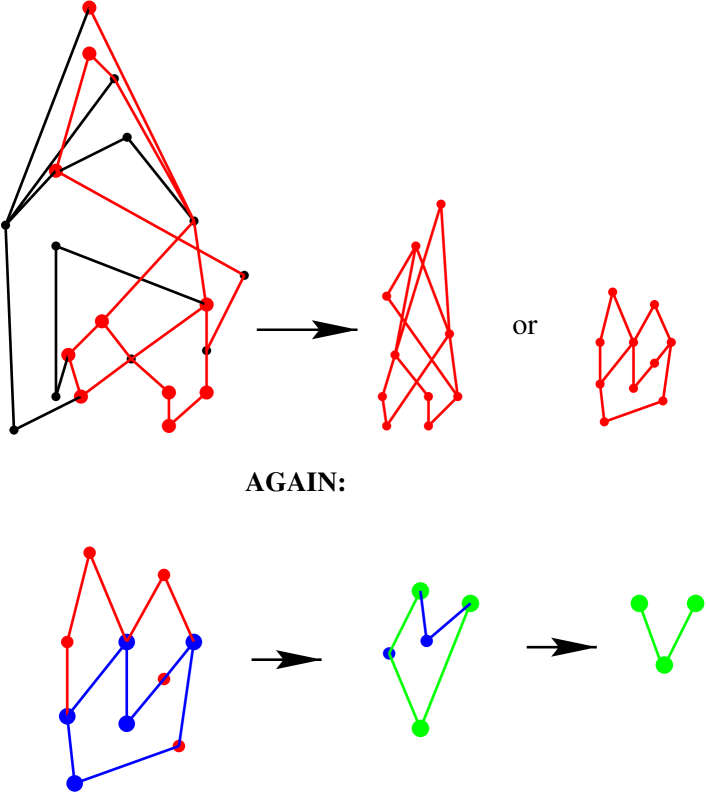
We see that, at the largest scale shown (i.e. the smallest number of remaining elements), $C$ has coarse-grained in this instance to the 3-element “V” causet.

1.3 Dynamics for Causal Sets

Because of their discrete character, many issues arise in causal set dynamics which are not present in the formulation of dynamics for continuum theories. Some general principles which need to be understood in a discrete context are general covariance, “manifoldness” (i.e. the emergence of a continuum at macroscopic length scales), and locality. This section will merely present some general issues which arise when attempting to express a dynamics for causal sets. A precise, detailed account follows in Chapter 3.

1.3.1 General covariance

An $N$ element partial order $P$ admits a natural labeling, which is an assignment of a non-negative integer $0,1,2,\ldots N-1$ to each element of $P$ such that $x\prec~{}y\Rightarrow\mathrm{label}(x)<\mathrm{label}(y)\;\>\forall\,x,y\in P$. Since a coordinate system in general relativity is simply an assignment of a “label” for each event of spacetime, a labeling of a causal set corresponds to a choice of coordinates in general relativity. The continuum analog of a natural labeling might be a coordinate system in which $x^{0}$ is everywhere timelike (and this in turn is almost the same thing as a foliation by spacelike slices). One can also consider an arbitrary labeling, which is an assignment of integers to the elements as above but in a manner irrespective of the causal order $\prec$. This would be more closely analogous to arbitrary coordinate systems. In that case, there would be a well-defined gauge group — the group of permutations of the causet elements — and labeling invariance would signify invariance under this group, in analogy with diffeomorphism invariance and ordinary gauge invariance. However, we have not found a useful way make use of this, and consider only natural labelings. In the context of causal sets, then, general covariance will translate into a statement of label independence of the dynamics.

The dynamics for causal sets will be expressed as a measure defined on suitably chosen classes of histories, which in the context of causal sets are just the causal sets themselves. Generally we think of these histories as having infinite cardinality, i.e. they extend arbitrarily far into the future. The issue of general covariance then serves to limit the sets of histories which have a physically meaningful measure, or equivalently, what are the physically meaningful questions one can ask of the theory.

In discussing this issue, it will be useful to first define the notion of a stem. A full stem of a causal set $C$ is a finite subcauset $S$ for which every element not in $S$ succeeds a maximal element of $S$. A full stem corresponds to a completed partial history of the universe. A partial stem of a causet $C$ is a finite subcauset $S$ which contains its own past, i.e. if $x\in S$ and $y\in C$ such that $y\prec x$ then $y\in S$.

An example of a non-generally covariant question is “What is the probability that the universe has a 3-chain as a full stem after $N$ elements appear.” This is not generally covariant because a labeling is implicit in the notion “after $N$ elements appear.” A covariant question could ask “What is the probability that the universe has a 3-chain as a full stem, after the growth process runs to completion”, i.e. in the limit as $N\rightarrow\infty$. It is conjectured that all physical questions can be expressed as a logical combination of probabilities of the occurrence of a given partial stem in the universe. Can a measure be formulated that assigns a finite answer to all such questions?

1.3.2 “Manifoldness”

Almost every causal set in no way resembles any spacetime manifold. To get a feel for how extreme this is, it has been shown that, in the limit of large $N$, the number of partial orders defined on $N$ elements grows as $2^{N^{2}/4}$ (to leading order). In comparison, one may estimate that the number of “spacetime resembling” posets on $N$ elements is only $\sim 2^{N\ln N}$. Somehow the dynamics must select those that (at least at a sufficiently large length scale) resemble spacetimes. One might expect this selection to occur at the classical level, i.e. in the classical limit “dynamically preferred” causets should faithfully embed into spacetimes. This limit arises from the constructive interference of histories, so the “spacetime resembling causets” should lie at “a stationary point in the causal set action”, while those that are very unlike continuua should have “rapidly varying” amplitudes. Of course one needs a precise notion of how causets are “close to each other” to be able to speak of a stationary point. Our intuition comes roughly from a notion of “closeness” for Lorentzian geometries.

A related question to the existence of a continuum is why the cosmological constant is so small. If it had it’s “natural” value, of 1 in Planck units, then spacetime would have curvature on scales of the Planck length, meaning that there is no continuum. Thus any theory of quantum gravity must provide some mechanism for driving $\Lambda$ to zero. Given that such a (relatively unknown) mechanism exists, causal sets provide a heuristic explanation for why $\lambda$ is not exactly zero, but fluctuates about zero with an amplitude which falls off as $1/\sqrt{N}$, where $N$ is the volume of the universe in fundamental units [55]. Given that for the current era $N\sim 10^{240}$, this predicts an order of magnitude that is consistent with current observation.

In addition, this problem is addressed in part by the renormalization type behavior of the dynamics and the existence of a continuum limit, discussed in Sections 2.3 and 2.4.

1.3.3 Locality

Whatever the microscopic dynamics for causal sets may look like, we expect that the continuum approximation will be governed by an effective Lagrangian

$$L_{\mathrm{eff}}\sim-\Lambda+\frac{R}{2\kappa}+(R^{2})+\cdots$$ (1.4)

where $(R^{2})$ represents terms involving the curvature squared, etc. Dimensional consistency indicates that the coefficient before each term gets smaller in the expansion, since the curvature $R$ has dimension $1/\mathrm{length}^{2}$, so each $R$ must have a coefficient of $l_{p}^{2}$, implying that the higher order terms have negligible contribution. However, this expression will be difficult to compute, even using the method of estimating curvature from counting in an interval mentioned in §1.2.4.3, because almost every Alexandrov set is “extremely null”.

However, the causal set is an inherently non-local object, so it is not unreasonable to expect that the notion of locality in the continuum will not carry over in an obvious, direct manner to the discrete dynamics. In fact the discrete dynamics, in its current formulation (see e.g. (3.23)), appears quite non-local, in that the “behavior” of a “region of the causal set” depends on its entire past.

Rather than directly trying to reproduce the action of (1.4) (say with some additional matter terms), an alternative approach is to get locality later, in the effective, continuum theory. Then the objective would be to use the notion of locality as a guide in choosing the microscopic dynamics, trying to determine what it means in this context, without worrying necessarily about getting an action as in (1.4). If we do manage to choose an effectively local microscopic dynamics, then the Einstein-Hilbert action will come out “for free”, given the dimensional arguments above (and local Lorentz invariance). For the case of causal sets, this approach seems more likely to bear fruit.

In general it is difficult to define a discrete “lattice” which is Lorentz invariant, as most regular lattices that one considers are not invariant under Lorentz transformations. However, the set of points obtained from a random “sprinkling” into a spacetime region is Lorentz invariant. Taking advantage of this property of a random embedding, progress has been made in understanding how an effectively local action may arise in the context of causal sets [23, 52]. Their work shows that Lorentz invariance can be made compatible with locality on a lattice.

This apparent success in combining locality, Lorentz invariance, and discreteness demonstrates a great advantage of causal sets. Never before have all these three aspects been present in a physical theory.

Chapter 2 Investigation of Transitive Percolation Dynamics

2.1 Introduction

The dynamics of causal sets will likely find its final expression as a quantum measure defined over suitably chosen classes of “histories”, where in this case a history will be simply a causal set. One may expect, in analog with the path integral formulation of quantum mechanics, that the quantum measure will arise from a sum over histories, which may have a form similar to

$$\sum_{C,C^{\prime}}A(C,C^{\prime};\{q\})$$ (2.1)

where $A$ is a complex amplitude for a pair of causal sets $C,C^{\prime}$, possibly depending on a set of parameters $\{q\}$. A difficulty in defining the quantum measure in terms of a sum of this nature is that the sum would likely have to be constrained to “Schwinger histories”, which are pairs of histories that have the same “value” at some time “$T$” which is to the future of any constraint which is used to define the set of histories for which one is seeking the measure. Because there is no covariant notion of a time $T$ in cosmology, and the notion of the “value” of a causal set at a “time $T$” is also difficult to define, it is difficult to see how to directly write down a measure of the form (2.1). Instead, the quantum measure will probably arise via a construction analogous to that which defines the classical measure (3.23).

Even though we do not know the exact form of the summand, a question which presents itself is how to enumerate the causal sets which form the domain of the sum itself. This problem has been studied extensively, often in the context partial orders as transitive, acyclic, directed graphs. In particular, Kleitman and Rothschild [34] (see also [19]) have shown that, in the asymptotic limit $N\rightarrow\infty$, the number of distinct orders definable on $N$ elements is given by

$$(1+O(1/N))\phi_{p}\frac{2^{3/4}}{\sqrt{\pi}}\,2^{N^{2}/4+3N/2-\log_{2}N/2}\>,$$

where

$$\phi_{p}=\sum_{j=-\infty}^{\infty}2^{-(j+1/2)^{2}}\approx 2.1289312\>$$

for even $N$ and

$$\phi_{p}=\sum_{j=-\infty}^{\infty}2^{-j^{2}}\approx 2.1289368$$

for odd $N$. Thus, for any appreciable value of $N$ (say $N>20$), in the absence of some special amplitude $A(C,C^{\prime};\{q\})$ which for example is zero on all but a vanishingly small fraction of the $N$-element causets, it seems that, in practice, the sum in (2.1) must performed by a simulation or other approximation method. An important question then is how to sample the set of $N$-element causets.

There exists a simple “model” for generating partially ordered sets at random, which is familiar in the field of random graph theory, which we call transitive percolation. The name, suggested by David Meyer [39], arises from the fact that this model can be regarded as a sort of one-dimensional directed percolation, where a relation $i\prec j$ is thought of as a “bond” or “channel” between “sites” $i$ and $j$ in a one dimensional lattice (c.f. e.g. [42]). It is defined by a single real parameter $p$ (and a non-negative integer $N$). To generate an $N$-element poset at random, start with a set of $N$ elements labeled $0,1,2,\ldots N-1$, and introduce a relation between each of the ${N\choose 2}$ pairs of elements with a probability $p$ (with the element with the smaller label preceding that with the greater), where $p$ is any real number in $[0,1]$. Since the resulting relation will not be transitive in general, form its transitive closure (e.g. if $2\prec 3$ and $3\prec 438$ then enforce that $2\prec 438$).

If transitive percolation is to be used to sample the domain of summation in (2.1), then we need to understand in detail the resulting distribution on the set of $N$-element causal sets, so a weight factor can be placed into the summand to correct for the bias of the sampling technique. Unfortunately, it is impossible to do this, for the following reason. The asymptotic enumeration of $N$-element orders found by Kleitman and Rothschild mentioned above was achieved by showing that almost all $N$-orders are “3-layer” orders. (An “$l$-layer order” is one in which the set of elements is partitioned into $l$ antichains $X_{1}$, $X_{2}$, $\ldots,X_{l}$, where each element of $X_{i}$ precedes every element of $X_{j}$ for $j>i+1$, and no element of $X_{i}$ precedes any element of $X_{j}$ for $i>j$.) Furthermore, they found that almost all 3-layer orders have about $N/2$ elements in $X_{2}$ and about $N/4$ elements in the other antichains. Here “almost all” means that the fraction of orders with this characteristic goes to 1 in the limit $N\rightarrow\infty$. This result tells us that essentially all posets sampled will be 3-layer, so that the weight factor will degenerate to zero for any non-3-layer posets, which bodes ill for the whole approach of doing a Monte-Carlo sum.

(In connection with generic, layered orders, Deepak Dhar [25] and Kleitman and Rothschild [35] have studied the behavior of an entropy function on these posets, $S(r)$, where $r$ is the ordering fraction defined in §1.2.3.2. They found an infinite number of first order phase transitions, at each of which $\partial S/\partial r$ vanishes over a finite interval of $r$. The order parameter is the average height, which increases by one across each transition. In addition, they have found that, for a given $r$, most causets are highly time-asymmetric. The presence of the phase transitions suggests that there may be a continuum limit.)

Obviously these 3-layer posets in no way resemble those which would faithfully embed into a spacetime. Since their number grows exponentially in $N^{2}$, one may imagine that any dynamics for causal sets is doomed to failure, since any Boltzmann-like weight which “only” grows exponentially in an extensive quantity (e.g. energy) would be insufficient to overcome this super-exponential entropic weight factor. Thus we have a sort of entropy catastrophe, forcing generic causets upon us regardless of our choice of dynamics. However, the causal sets generated by the transitive percolation algorithm look nothing like the generic 3-layer orders. If this model is to be regarded as a physical dynamics in itself, then this entropy catastrophe is already forestalled with this quite naive dynamical model. In fact, we can see that the dynamics of causal sets, being inherently non-local, would be expected to have an action which grows quadratically with an extensive quantity, rather than linearly. Then this sort of non-local action is exactly what is needed to overcome the entropic dominance of the generic orders. (In fact, the probability of arriving at a causal set with $R$ related pairs, via the transitive percolation algorithm, grows like $e^{\beta R}$, where $\beta=-\ln p$ acts as a sort of inverse temperature. c.f. [24]) Note that this situation is not so different from that of ordinary quantum mechanics, where the smooth paths, which form a set of measure zero in the space of all paths, are the ones which dominate the sum over histories in the classical limit.

One important question which has not been addressed is at what value of $N$ the Kleitman Rothschild result becomes valid. Enumeration of partial orders by computer shows no obvious tendency toward the 3-layer orders, for the meager values of $N$ which a computer allows. It is possible, however unlikely, that the result will be of no consequence for causal sets, as it emerges only after $N$ is much larger than will ever be needed for physically reasonable causal sets, say $N\gg 10^{240}$. In any event it would be useful to have a feel for the “domain of validity” of this asymptotic result.

We will see that in fact transitive percolation can be regarded as much more than just an algorithm to generate causal sets at random to be used in a Monte-Carlo sum over histories. It is an important special case of a generic class of “sequential growth” dynamics for causal sets, which will be explained in detail in Chapter 3. In particular, it has many appealing features, both as a model for a relatively small region of spacetime and as a cosmological model for spacetime as a whole. Incidentally, it has attracted the interest of both mathematicians and physicists for reasons having nothing to do with quantum gravity. By physicists, it has been studied as a problem in the statistical mechanical field of percolation. By mathematicians, it has been studied extensively as a branch of random graph theory (a poset being the same thing as a transitive acyclic directed graph). Conversely, random graph theory could be construed as the theory of percolation on a complete graph. Some physics references on transitive percolation are [42, 24, 50, 48]. In connection with random graph theory, there exist a large number of results governing the asymptotic behavior of posets generated in this manner [17, 13, 12, 11, 45, 22, 33, 53, 2].

2.2 Features

2.2.1 May resemble continuum spacetime

In computer simulations, two independent coarse-graining invariant dimension indicators, Myrheim-Meyer dimension and midpoint scaling dimension, tend to agree with each other, which is encouraging if these causal sets are to embed faithfully into spacetime with a well defined dimension. Another dimension indicator, which involves counting small subcausets whose frequency provides an indicator of dimension, behaves poorly. However, this measure of dimension is not invariant under coarse graining, so it only indicates that transitive percolated causal sets themselves do not directly embed faithfully into Minkowski space, but some appropriately chosen subcauset (e.g. coarse-grained) may still approximate a spacetime, which is what one would expect for a dynamics of causal sets anyway.

In the pure percolation model, however, these dimension indicators vary with time (i.e. with $N$, as the causal set “grows”) which suggests that one may wish to rescale $p$ in such a way as to hold the spacetime dimension constant. One may ask, then, if the model can be generalized by having $p$ vary with $N$ in an appropriate sense. We will see in Chapter 3 that something rather like this is in fact possible.

2.2.2 Homogeneous

Consider the transitive percolation algorithm described in §2.1, and an arbitrary element of a causal set generated by this model, say the one labeled 257. Its future will be some causal set, $\mathrm{future}(257)$. Because of the extreme symmetry of the transitive percolation algorithm, the probability distribution of $\mathrm{future}(257)$ will be completely independent of the structure of that portion of the causal set which is to the past of element 257, or spacelike to 257. This is clear because, regardless of what is to the past and unrelated to this element, each successive element will join to 257 with a fixed probability $p$. Thus its future will behave the same as that of any of the other elements.

Therefore, the only spacetimes which a causal set generated by transitive percolation could hope to resemble would be (space-time) homogeneous, such as the Minkowski, de Sitter, or anti-de Sitter spacetimes. Likewise transitive percolation has no hope of resembling a spacetime with propagating degrees of freedom, such as gravitational waves.

2.2.3 Time reversal invariance

Transitive percolation is independent of time orientation. When viewed from the perspective of a sequential growth dynamics, this may not be so obvious, but it is clear when viewed from the more static algorithm described above.

2.2.4 Existence of a continuum limit

Moreover, computer simulations suggest strongly that the model possesses a continuum limit (see Section 2.3) and exhibits scaling behavior in that limit with $p$ scaling roughly like $c\log{n}/n$ [48].

2.2.5 Originary transitive percolation

There exists another model which is very similar to transitive percolation, called “originary transitive percolation”. It is most clearly described in terms of a “cosmological growth process” which is introduced in §3.1.1. For now, suffice it to say that the model is the same as transitive percolation, except that every element (but one) must be a descendent of at least one other element of the causet. The net effect is that the growing causal set is required to have an “origin” (= unique minimum element). It turns out that originary transitive percolation is equivalent to ordinary transitive percolation, if one “discards” all elements which are not to the future of the first element. That is, if one generates a causet via transitive percolation with $N$ and $p$, and then considers only the subcauset which contains the (inclusive) future of “element 0”, one obtains a model equivalent to that of originary transitive percolation at the same $p$ (but of course smaller $N$).

2.2.6 Suggestive large scale cosmology

Consider a picture of causal set cosmology which involves cosmological “bounces”, where the causal set collapses down to a single element, and then re-expands as illustrated in Figure 2.1.

Figure 2.1: Transitive percolation cosmology

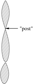
Alon et al. [2] call such an element a post, which is defined as an element which is related to every other in the causal set. In the context of percolation dynamics, they have proved rigorously that such cosmological bounces occur with probability 1 (if $p>0$), from which it follows that there are infinitely many cosmological cycles, each cycle but the first having the dynamics of originary percolation. Then the “cosmology” of transitive percolation is quite suggestive, consisting of a universe which cycles endlessly through phases of expansion, stasis, and contraction (via fluctuation) back down to a single element.

Note that transitive percolation is only homogeneous on average. Thus, with this stochastic model, we see a phenomenon which does not arise in deterministic theories — a “locally homogeneous spacetime” which nevertheless possesses points where the universe contracts to “volume 1” and reexpands. Also, this means that transitive percolation cannot produce the entirety of an Einstein spacetime, it is only possible that its continuum limit yield a portion of some homogeneous spacetime.

2.2.7 Cosmological renormalization

In Chapter 3, the classical dynamics for causal sets will be expressed in terms of a countable sequence of parameters, or “coupling constants”, $t_{n}$. Some work by Dou [26], and more recently [59, 38], describes a “cosmological renormalization” process, wherein at each cycle of expansion, collapse to a single point, and re-expansion, the parameters describing the dynamics of the causal set are “renormalized”, taking new effective values in each subsequent cycle. It is easy to show that the percolation dynamics are the unique “fixed points” under this renormalization flow, and furthermore that a large class of dynamics (choices for the parameters $t_{n}$) converge to this fixed point as the renormalization process extends to infinity. Thus, if our universe is in fact described by something resembling the dynamics to be derived in Chapter 3, and it does undergo cycles of expansion and re-contraction, then after a long time it will be increasingly described by this (originary) transitive percolation dynamics.

Furthermore, if the parameters $t_{n}$ take the form given in (3.19), which might be expected for a physically reasonable dynamics, then the cosmological renormalization process makes an interesting “prediction” regarding the early universe. As discussed in [59], for the dynamics of (3.19), the early universe behaves as originary transitive percolation for a period which grows longer and longer after successive cosmological renormalizations. In addition, the effective $p$ of this percolation phase diminishes as $1/\sqrt{N}$, with $N$ being the number of elements to the past of the current cosmological epoch. Thus after a long time, $p$ will be driven to an arbitrarily small value. If this is the case, then it can provide some explanation to the puzzle of why the universe is so large, homogeneous, and isotropic. The reason is that, for extremely small $p$, originary percolation will almost surely generate a “Cayley tree”, which is a tree for which each element has on average two immediate successors. After this rapidly expanding “tree phase” the universe should make a transition into something resembling a spacetime which is spatially homogeneous and isotropic.

2.2.8 Phase transitions in the early universe

For the (non-originary) transitive percolation dynamics, it is known that there is a percolation phase transition at $p\sim{1/N}$, where the causet transforms qualitatively from a large number of small disconnected universes for $p<p_{\mathrm{crit}}$ to a causet with one large universe and a number of much smaller disconnected universes for $p>p_{\mathrm{crit}}$. (This can be regarded as the “early universe” of transitive percolation because cosmological time can be measured by spacetime volume, so that small $N$ corresponds to short or early times.) A second phase transition gathers the disconnected branches of the universe, leading to a single connected universe. This occurs near the percolation transition, at $p\sim\ln N/N$ [45]. In fact, this second phase transition occurs “at the same time” as a third, at which the fraction of elements to the future of element 0 becomes very close to 1.

There is, incidentally, still some hope of being able to reproduce the generic 3-layer posets by running the transitive percolation algorithm at the percolation phase transition. It is possible that each piece (connected component) of the causet would be a generic poset.

2.2.9 Diffusion-like model

The expectation value of the ordering fraction $<\!r\!>$ of a causet generated by transitive percolation can be computed exactly by writing a recursion relation for the number of descendants of element 0 (we’ll call this element $e_{0}$ for short). For the purposes of this discussion we switch to the reflexive convention for defining a partial order, i.e. replace the irreflexivity condition $x\not\prec x$ with reflexivity $x\prec x$ (and re-impose acyclicity with $x\prec y\prec x\Rightarrow x=y$). Define $f_{n}(k)$ to be the probability that, considering only those elements whose labels are less than $n$, $e_{0}$ has exactly $k$ descendents. Clearly $f_{1}(k)=\delta_{1}^{k}$. The recursion relation can be defined by noting that “at stage $n$”, there are two ways that $e_{0}$ can have $k$ descendents. “At stage $n-1$” either $e_{0}$ had $k$ descendents, and element $n$ does not “link to” any element to the future of $e_{0}$, or $e_{0}$ had $k-1$ descendents, and element $n$ does link to one of $e_{0}$’s descendents. The former event occurs with probability $q^{k}$, while the latter with probability $1-q^{k-1}$. Thus

$$f_{n}(k)=q^{k}f_{n-1}(k)+(1-q^{k-1})f_{n-1}(k-1)\>.$$ (2.2)

The expected number of descendents of $e_{0}$ “at stage $n$” is then

$$x_{n}=\sum_{k=1}^{n}kf_{n}(k)\>.$$

Because of the symmetry of the percolation algorithm, the expected number of descendents of element 1 at stage $n$ is equivalent to the expected number of descendents of element 0 at stage $n-1$. (To see this, simply relabel the causet such that element $i$ is relabeled $i-1$.) Then the expected number of relations in an $N$-element percolated causet, is $\sum_{n=1}^{N}x_{n}$, or switching back to the irreflexive convention,

$$<\!R(N)\!>=\sum_{n=1}^{N}(x_{n}-1)\>.$$

This recursion relation can be evaluated quite efficiently on a computer, to yield values of $<\!r\!>$, so far for $N$ up to $2^{21}$, accurate to numerical rounding errors.

If this Markov process is modeled by a differential equation, the “field” $f$ behaves as a wave moving at constant speed “to the right”, with a diffusive character. It is possible that further study along these lines will lead to an understanding of the asymptotic behavior of this model, for example to understand the scaling behavior discussed in §2.4.

A generalization of this recursion relation is possible for the originary percolation model, but it is more expensive computationally than the $O(N^{2})$ algorithm described here.

2.2.10 Gibbsian distribution

Transitive percolation is readily embedded in a “two-temperature” statistical mechanics model, and as such, happens also to be “exactly soluble” in the sense that the partition function can be computed exactly. Details of this model will be described in [24].

2.3 Continuum Limit

Here we search for evidence of a continuum limit in the transitive percolation dynamics. One might question whether a continuum limit is even desirable in a fundamentally discrete theory, but a continuum approximation in a suitable regime is certainly necessary if the theory is to reproduce known physics. Given this, it seems only a small step to a rigorous continuum limit, and conversely, the existence of such a limit would encourage the belief that the theory is capable of yielding continuum physics with sufficient accuracy.

Perhaps an analogy with kinetic theory can provide a useful illustration. In quantum gravity, the discreteness scale is set, presumably, by the Planck length $l=(\kappa\hbar)^{1/2}$ (where $\kappa=8\pi{G}$), whose vanishing therefore signals a continuum limit. In kinetic theory, the discreteness scales are set by the mean free path $\lambda$ and the mean free time $\tau$, both of which must go to zero for a description by partial differential equations to become exact. Corresponding to these two independent length and time scales are two “coupling constants”: the diffusion constant $D$ and the speed of sound $c_{\mathrm{sound}}$. Just as the value of the gravitational coupling constant $G\hbar$ reflects (presumably) the magnitude of the fundamental spacetime discreteness scale, so the values of $D$ and $c_{\mathrm{sound}}$ reflect the magnitudes of the microscopic parameters $\lambda$ and $\tau$ according to the relations

$$D\sim{\lambda^{2}\over\tau},\quad c_{\mathrm{sound}}\sim{\lambda\over\tau}$$

or conversely

$$\lambda\sim{D\over c_{\mathrm{sound}}},\quad\tau\sim{D\over c_{\mathrm{sound}}^{2}}\,.$$

In a continuum limit of kinetic theory, therefore, we must have either $D\rightarrow 0$ or $c_{\mathrm{sound}}\rightarrow\infty$. In the former case, we can hold $c_{\mathrm{sound}}$ fixed, but we get a purely mechanical macroscopic world, without diffusion or viscosity. In the latter case, we can hold $D$ fixed, but we get a “purely diffusive” world with mechanical forces propagating at infinite speed. In each case we get a well defined — but defective — continuum physics, lacking some features of the true, atomistic world.

If we can trust this analogy, then something very similar must hold in quantum gravity. To send $l$ to zero, we must make either $G$ or $\hbar$ vanish. In the former case, we would expect to obtain a quantum world with the metric decoupled from non-gravitational matter; that is, we would expect to get a theory of quantum field theory in a purely classical background spacetime solving the source-free Einstein equations. In the latter case, we would expect to obtain classical general relativity. Thus, there might be two distinct continuum limits of quantum gravity, each physically defective in its own way, but nonetheless well defined.

For our purposes, the important point is that, although we would not expect quantum gravity to exist as a continuum theory, it could have limits which do, and one of these limits might be classical general relativity. It is thus sensible to inquire whether one of the classical causal set dynamics we have defined describes classical spacetimes. In the following, we make a beginning on this question by asking whether the special case of “percolated causal sets”, as we will call them, admits a continuum limit at all.

Of course, the physical content of any continuum limit we might find will depend on what we hold fixed in passing to the limit, and this in turn is intimately linked to how we choose the coarse-graining procedure that defines the effective macroscopic theory whose existence the continuum limit signifies. Obviously, we will want to send $N\rightarrow\infty$ for any continuum limit, but it is less evident exactly how we should coarse-grain and what coarse grained parameters we want to hold fixed in taking the limit. Indeed, the appropriate choices will depend on whether the macroscopic spacetime region we have in mind is, to take some naturally arising examples, ($i$) a fixed bounded portion of Minkowski space of some dimension, ($ii$) an entire cycle of a Friedmann universe from initial expansion to final recollapse, or ($iii$) an $N$-dependent portion of an unbounded spacetime $M$ that expands to encompass all of $M$ as $N\rightarrow\infty$. In the sequel, we will have in mind primarily the first of the three examples just listed. Without attempting an definitive analysis of the coarse-graining question, we will simply adopt the simplest definitions that seem to us to be suited to this example. More specifically, we will coarse-grain by the random selection procedure of §1.2.6, and we will choose to hold fixed some convenient invariants of that sub-causal-set, including the ordering fraction, which, as mentioned in §1.2.3.2, can be interpreted as the dimension of the spacetime region it constitutes. As we will see, the resulting scheme has much in common with the kind of coarse-graining that goes into the definition of continuum limit in quantum field theory. For this reason, we believe it can serve also as an instructive “laboratory” in which this concept, and related concepts like “running coupling constant” and “non-trivial fixed point”, can be considered from a fresh perspective.

2.3.1 The critical point at $p=0$, $N=\infty$

Transitive percolation is a model of random causets which depends on two parameters, $p\in[0,1]$ and $N\in\hbox{\openface N}$. For a given $p$, the model defines a probability distribution on the set of $N$-element causets. For $p=0$, the only causet with nonzero probability, obviously, is the $N$-antichain. Now let $p>0$. With a little thought, one can convince oneself that for $N\rightarrow\infty$, the causet will look very much like a chain. Indeed it has been proved [7] (see also [42]) that, as $N\rightarrow\infty$ with $p$ fixed at some (arbitrarily small) positive number, $r\rightarrow 1$ in probability, where $r$ is the ordering fraction of the causal set. Note that the $N$-chain has the greatest possible number of relations ${N\choose 2}$, so $r\rightarrow 1$ gives a precise meaning to “looking like a chain”.

We see that for $N\rightarrow\infty$, there is a change in the qualitative nature of the causet as $p$ varies away from zero, and the point $p=0,N=\infty$ (or $p=1/N=0$) is in this sense a critical point of the model. It is the behavior of the model near this critical point which we study in detail.

The fact that a coarse grained causet is automatically another causet will make it easy for us to formulate precise notions of continuum limit, running of the coupling constant $p$, etc. In this respect, we believe that this model combines precision with novelty in such a manner as to furnish an instructive illustration of concepts related to renormalizability, independently of its application to quantum gravity.

2.3.2 The large scale effective theory

The transitive percolation model for generating random causal sets is a “microscopic” dynamics, and the procedure described in §1.2.6 provides a precise notion of coarse graining (that of random selection of a sub-causal-set). On this basis, we can produce an effective “macroscopic” dynamics by imagining that a causet $C$ is first percolated with $N$ elements and then coarse-grained down to $m<N$ elements. This two-step process constitutes an effective random procedure for generating $m$ element causets depending (in addition to $m$) on the parameters $N$ and $p$. In causal set theory, number of elements corresponds to spacetime volume, so we can interpret $N/m$ as the factor by which the “observation scale” has been increased by the coarse graining. If, then, $V_{0}$ is the macroscopic volume of the spacetime region constituted by our causet, and if we take $V_{0}$ to be fixed as $N\rightarrow\infty$, then our procedure for generating causets of $m$ elements provides the effective dynamics at volume-scale $V_{0}/m$ (i.e. length scale $(V_{0}/m)^{1/d}$ for a spacetime of dimension $d$).

What does it mean for our effective theory to have a continuum limit in this context? Our stochastic microscopic dynamics gives, for each choice of $p$, a probability distribution on the set of causal sets $C$ with $N$ elements, and by choosing $m$, we determine at which scale to examine the corresponding effective theory. This effective theory is itself just a probability distribution $f_{m}$ on the set of $m$-element causets, so our dynamics will have a well defined continuum limit if there exists, as $N\rightarrow\infty$, a trajectory $p~{}=~{}p(N)$ along which the corresponding probability distributions $f_{m}$ on coarse grained causets approach fixed limiting distributions $f_{m}^{\infty}$ for all $m$. The limiting theory in this sense is then a sequence of effective theories, one for each $m$, all fitting together consistently. (Thanks to the associative (semi-group) character of our coarse-graining procedure, the existence of a limiting distribution for any given $m$ implies its existence for all smaller $m$. Thus it suffices that a limiting distribution $f_{m}$ exist for $m$ arbitrarily large.) In general there will exist not just a single such trajectory $p=p(N)$, but a one-parameter family of them (corresponding to the one real parameter $p$ that characterizes the microscopic dynamics at any fixed $N$), and one may wonder whether all the trajectories will take on the same asymptotic form as they approach the critical point $p=1/N=0$. The asymptotic form of this trajectory has been studied extensively in the mathematics literature [45, 13, 8, 7, 1, 33, 3, 2], with a variety of motivations, including for example the search for efficient sorting algorithms.

Consider first the simplest nontrivial case, $m=2$. Since there are only two causal sets of size two, the 2-chain and the 2-antichain, the distribution $f_{2}$ that gives the “large scale physics” in this case is described by a single number which we can take to be $f_{2}(\,\,\begin{picture}(0.0,1.0)\put(0.0,0.0){\circle*{0.6}}\put(0.0,1.0){\circle*{0.6}} \put(0.0,0.0){\line(0,1){1.0}} \end{picture}\,\,)$, the probability of obtaining a 2-chain rather than a 2-antichain. (The other probability, $f_{2}(\,\begin{picture}(1.0,1.0)\put(0.0,0.5){\circle*{0.6}}\put(1.0,0.5){\circle*{0.6}} \end{picture}\,\,\,)$, is of course not independent, since classical probabilities must add up to unity.) Interestingly enough, the number $f_{2}(\,\,\begin{picture}(0.0,1.0)\put(0.0,0.0){\circle*{0.6}}\put(0.0,1.0){\circle*{0.6}} \put(0.0,0.0){\line(0,1){1.0}} \end{picture}\,\,)$ has a direct physical interpretation in terms of the Myrheim-Meyer dimension of the fine-grained causet $C$. Indeed, it can be seen that $f_{2}(\,\,\begin{picture}(0.0,1.0)\put(0.0,0.0){\circle*{0.6}}\put(0.0,1.0){\circle*{0.6}} \put(0.0,0.0){\line(0,1){1.0}} \end{picture}\,\,)$ is nothing but the expectation value of what we called above the ordering fraction $r$ of $C$ (an argument explaining why this is so follows in the next section). But the ordering fraction, in turn, determines the Myrheim-Meyer dimension $d$ that indicates the dimension of the Minkowski spacetime $\hbox{\openface M}^{d}$ (if any) in which $C$ would embed faithfully as an interval [40, 41]. Thus, by coarse graining down to two elements, we are effectively measuring a certain kind of spacetime dimensionality of $C$. In practice, we would not expect $C$ to embed faithfully without some degree of coarse-graining, but the original $r$ would still provide a good dimension estimate since it is, on average, coarse-graining invariant.

As we begin to consider coarse-graining to sizes $m>2$, the degree of complication grows rapidly, simply because the number of partial orders defined on $m$ elements grows rapidly with $m$. For $m=3$ there are five possible causal sets:     ,     ,     ,     , and    . Thus the effective dynamics at this “scale” is given by five probabilities (so four free parameters). For $m=4$ there are sixteen probabilities, for $m=5$ there are sixty-three, and for $m=6$, 7 and 8, the number of probabilities is respectively 318, 2045, and 16999.

2.3.3 Evidence from simulations

In order that a continuum limit exist, it must be possible to choose a trajectory for $p$ as a function of $N$ so that the resulting coarse-grained probability distributions, $f_{1}$, $f_{2}$, $f_{3}$, …, have well defined limits as $N\rightarrow\infty$. To study this question numerically, one can simulate transitive percolation using the algorithm described in Section 2.1, while choosing $p$ so as to hold constant (say) the $m=2$ distribution $f_{2}$ ($f_{1}$ being trivial). Because of the way transitive percolation is defined, it is intuitively obvious that $p$ can be chosen to achieve this, and that in doing so, one leaves $p$ with no further freedom. (Observe that $<\!r\!>=f_{2}(\,\,\begin{picture}(0.0,1.0)\put(0.0,0.0){\circle*{0.6}}\put(0.0,1.0){\circle*{0.6}} \put(0.0,0.0){\line(0,1){1.0}} \end{picture}\,\,)$ is 0 when $p=0$, 1 when $p=1$, and increases smoothly and monotonically with $p$. Thus for any choice of $<\!r\!>\in[0,1]$ there must a $p$ which yields that $<\!r\!>$, and since $f_{2}(\,\begin{picture}(1.0,1.0)\put(0.0,0.5){\circle*{0.6}}\put(1.0,0.5){\circle*{0.6}} \end{picture}\,\,\,)=1-f_{2}(\,\,\begin{picture}(0.0,1.0)\put(0.0,0.0){\circle*{0.6}}\put(0.0,1.0){\circle*{0.6}} \put(0.0,0.0){\line(0,1){1.0}} \end{picture}\,\,)$, the entire distribution $f_{2}$.) The decisive question then is whether, along the trajectory thereby defined, the higher distribution functions, $f_{3}$, $f_{4}$, etc. all approach nontrivial limits.

As mentioned above, holding $f_{2}$ fixed is the same thing as holding fixed the expectation value $<\!r\!>$ of ordering fraction $r=R/{{N}\choose{2}}$. To see in more detail why this is so, consider the coarse-graining that takes us from the original causet $C_{N}$ of $N$ elements to a causet $C_{2}$ of two elements. Since coarse-graining is just random selection, the probability $f_{2}(\,\,\begin{picture}(0.0,1.0)\put(0.0,0.0){\circle*{0.6}}\put(0.0,1.0){\circle*{0.6}} \put(0.0,0.0){\line(0,1){1.0}} \end{picture}\,\,)$ that $C_{2}$ turns out to be a 2-chain is just the probability that two elements of $C_{N}$ selected at random form a 2-chain rather than a 2-antichain. In other words, it is just the probability that two elements of $C_{N}$ selected at random are causally related. Plainly, this is the same as the fraction of pairs of elements of $C_{N}$ such that the two members of the pair form a relation $x\prec{y}$ or $y\prec{x}$. Therefore, the ordering fraction $r$ equals the probability of getting a 2-chain when coarse graining $C_{N}$ down to two elements; and $f_{2}(\,\,\begin{picture}(0.0,1.0)\put(0.0,0.0){\circle*{0.6}}\put(0.0,1.0){\circle*{0.6}} \put(0.0,0.0){\line(0,1){1.0}} \end{picture}\,\,)=<\!r\!>$, as claimed.

This reasoning illustrates, in fact, how one can in principle determine any one of the distributions $f_{m}$ by answering the question, “What is the probability of getting this particular $m$-element causet from this particular $N$-element causet if you coarse grain down to $m$ elements?” To compute the answer to such a question starting with any given causet $C_{N}$, one examines every possible combination of $m$ elements, counts the number of times that the combination forms the particular causet being looked for, and divides the total by ${N\choose m}$. The ensemble mean of the resulting abundance, as we will refer to it, is then $f_{m}(\xi)$, where $\xi$ is the causet for which one is looking. In practice, of course, we normally use a more efficient counting algorithm than simply examining individually all ${N\choose m}$ subsets of $C_{N}$.

2.3.3.1 Histograms of 2-chain and 4-chain abundances

Figure 2.2: Distribution of number of relations for $N=4096$, $p=0.01155$

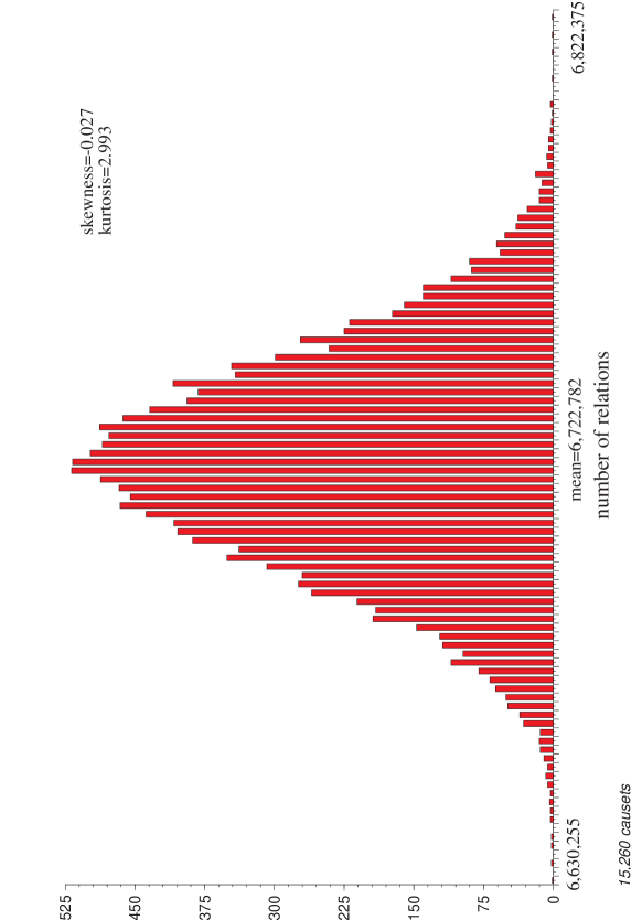
As explained in the previous subsection, the main computational problem, once the random causet has been generated, is determining the number of subcausets of different sizes and types. To get a feel for how some of the resulting “abundances” are distributed, we start by presenting a couple of histograms. Figure 2.2 shows the number $R$ of relations obtained from a simulation in which 15,260 causal sets were generated by transitive percolation with $p=0.01155$, $N=4096$. Visually, the distribution is Gaussian, in agreement with the fact that its “kurtosis”

$$\overline{\left(x-\overline{x}\right)^{4}}\,\bigg{/}\ {\overline{\left(x-\overline{x}\right)^{2}}\,}^{2}$$

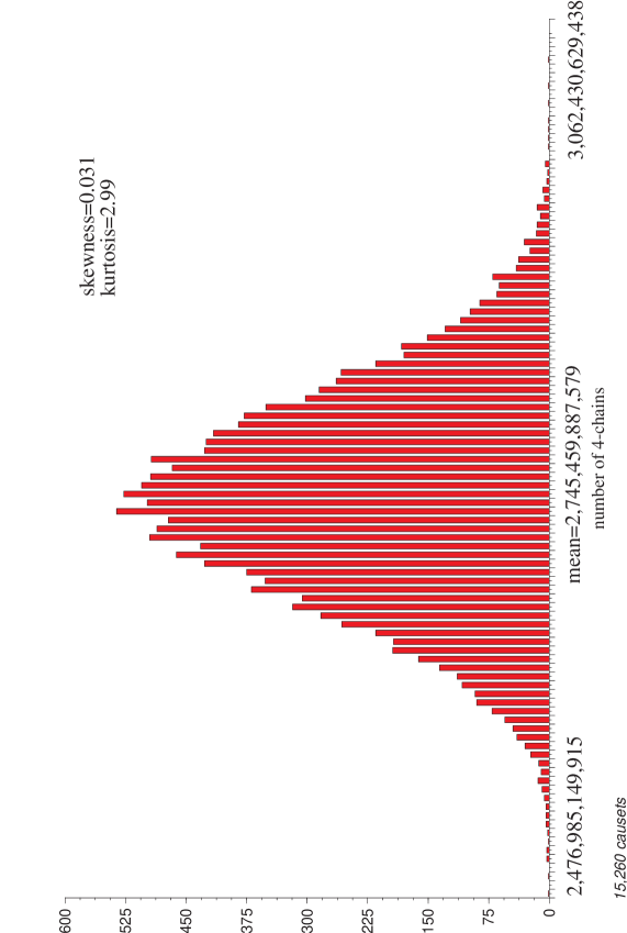
of 2.993 is very nearly equal to its Gaussian value of 3 (the over-bar denotes sample mean). In these simulations, $p$ was chosen so that the number of 3-chains was equal on average to half the total number possible, i.e. the “abundance of 3-chains”, $\mbox{(number of 3-chains)}/{N\choose 3}$, was equal to $1/2$ on average. The picture is qualitatively identical if one counts 4-chains rather than 2-chains, as exhibited in Fig. 2.3.

Figure 2.3: Distribution of number of 4-chains for $N=4096$, $p=0.01155$

(One may wonder whether it was to be expected that these distributions would appear to be so normal. If the variable in question, here the number of 2-chains $R$ or the number of 4-chains ($C_{4}$, say), can be expressed as a sum of independent random variables, then the central limit theorem provides an explanation. So consider the variables $x_{ij}$ which are 1 if $i\prec j$ and zero otherwise. Then $R$ is easily expressed as a sum of these variables:

$$R=\sum_{i<j}x_{ij}$$

However, the $x_{ij}$ are not independent, due to transitivity. Apparently, this dependence is not large enough to interfere much with the normality of their sum. The number of 4-chains $C_{4}$ can be expressed in a similar manner

$$C_{4}=\sum_{i<j<k<l}x_{ij}x_{jk}x_{kl}\,.$$

and similar remarks apply.)

Let us mention that for values of $p$ sufficiently close to 0 or 1, these distributions will appear skew. This occurs simply because the numbers under consideration (e.g. the number of $m$-chains) are bounded between zero and $N\choose m$ and must deviate from normality if their mean gets too close to a boundary relative to the size of their standard deviation. Whenever we draw an error bar in the following, we will ignore any deviation from normality in the corresponding distribution.

Notice incidentally that the total number of 4-chains possible is ${4096\choose 4}=11,710,951,848,960$. Consequently, the mean 4-chain abundance in our simulation is only $\frac{2,745,459,887,579}{11,710,951,848,960}=0.234$, a considerably smaller value than the mean 2-chain abundance of $<\!r\!>=\frac{6,722,782}{{4096\choose 2}}=0.802$. This was to be expected, considering that the 2-chain is one of only two possible causets of its size, while the 4-chain is one out 16 possibilities. (Notice also that 4-chains are necessarily less probable than 2-chains, because every coarse-graining of a 4-chain is a 2-chain, whereas the 2-chain can come from every 4-element causet save the 4-antichain.)

2.3.3.2 Trajectories of $p$ versus $N$

The question we are exploring is whether there exist, for $N\rightarrow\infty$, trajectories $p=p(N)$ along which the mean abundances of all finite causets tend to definite limits. To seek such trajectories numerically, we will select some finite “reference causet” and determine, for a range of $N$, those values of $p$ which maintain its mean abundance at some target value. If a continuum limit does exist, then it should not matter in the end which causet we select as our reference, since any other choice (together with a matching choice of target abundance) should produce the same trajectory asymptotically. We would also anticipate that all the trajectories would behave similarly for large $N$, and that, in particular, either all would lead to continuum limits or all would not. In principle it could happen that only a certain subset led to continuum limits, but we know of no reason to expect such an eventuality. In the simulations reported here, I have chosen as our reference causets the 2-, 3- and 5-chains. I have computed six trajectories, holding the mean 2-chain abundance fixed at 1/2, 1/3, and 1/10, the mean 3-chain abundance fixed at 1/2 and .0814837, and the mean 5-chain abundance fixed at 1/2. For $N$, I have used as large a range as available computing resources allowed.

Figure 2.4: Ordering fractions as a function of $p$ for $N=2048$

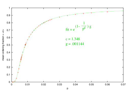
Before discussing the trajectories as such, let us have a look at how the mean 2-chain abundance $<\!r\!>$ (i.e. the mean ordering fraction) varies with $p$ for a fixed $N$ of 2048, as exhibited in Figure 2.4. (Vertical error bars are displayed in the figure but are so small that they just look like horizontal lines. The plotted points were obtained from the exact calculation for the ensemble average $<\!r\!>$ discussed in §2.2.9, so the errors come only from floating point roundoff. The fitting function used in Figure 2.4 will be discussed in [48]. As one can see, $<\!r\!>$ starts at 0 for $p=0$, rises rapidly to near 1 and then asymptotes to 1 at $p=1$ (not shown). Of course, it was evident a priori that $<\!r\!>$ would increase monotonically from 0 to 1 as $p$ varied between these same two values, but it is perhaps noteworthy that its graph betrays no sign of discontinuity or non-analyticity (no sign of a “phase transition”). To this extent, it strengthens the expectation that the trajectories we find will all share the same qualitative behavior as $N\rightarrow\infty$.

Figure 2.5: Flow of the “coupling constant” $p$ as $N\rightarrow\infty$ (six trajectories)

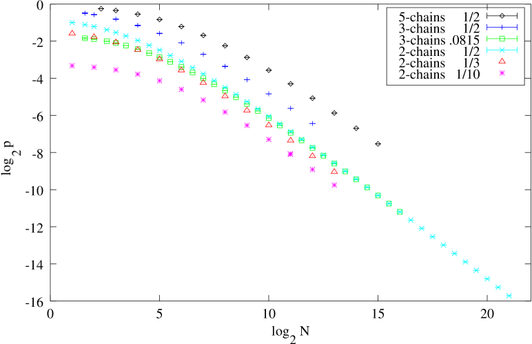
The six trajectories we have simulated are depicted in Fig. 2.5. A higher abundance of $m$-chains for fixed $m$ leads to a trajectory with higher $p$. Also note that, as observed above, the longer chains require larger values of $p$ to attain the same mean abundance, hence a choice of mean abundance = 1/2 corresponds in each case to a different trajectory. The trajectories with $<\!r\!>$ held to lower values are “higher dimensional” in the sense that $<\!r\!>=1/2$ corresponds to a Myrheim-Meyer dimension of 2, while $<\!r\!>=1/10$ corresponds to a Myrheim-Meyer dimension of 4. Observe that the plots give the impression of becoming straight lines with a common slope at large $N$. This tends to corroborate the expectation that they will exhibit some form of scaling with a common exponent, a behavior reminiscent of that found with continuum limits in many other contexts. This is further suggested by the fact that two distinct trajectories ($f_{2}(\,\,\begin{picture}(0.0,1.0)\put(0.0,0.0){\circle*{0.6}}\put(0.0,1.0){\circle*{0.6}} \put(0.0,0.0){\line(0,1){1.0}} \end{picture}\,\,)=1/2$ and $f_{3}(\,\,\begin{picture}(0.0,2.0)\put(0.0,0.0){\circle*{0.6}}\put(0.0,1.0){\circle*{0.6}}\put(0.0,2.0){\circle*{0.6}} \put(0.0,0.0){\line(0,1){2.0}} \end{picture}\,\,)=.0814837$), obtained by holding different abundances fixed, seem to converge for large $N$.

Figure 2.6: Six trajectories approaching the critical point at $p=0$, $N=\infty$

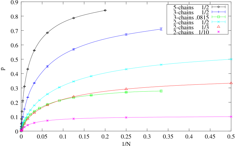
By taking the abscissa to be $1/N$ rather than $\log_{2}N$, we can bring the critical point to the origin, as in Fig. 2.6. The lines which pass through the data points there are just splines drawn to aid the eye in following the trajectories. Note that the curves tend to asymptote to the $p$-axis, suggesting that $p$ falls off more slowly than $1/N$. This suggestion is corroborated by more detailed analysis of the scaling behavior of these trajectories, as will be discussed in [48].

2.3.3.3 Flow of the coarse-grained theory along a trajectory

We come finally to a direct test of whether the coarse-grained theory converges to a limit as $N\rightarrow\infty$. Independently of scaling or any other indicator, this is by definition the criterion for a continuum limit to exist. I have examined this question by means of simulations conducted for five of the six trajectories mentioned above. In each simulation I proceeded as follows. For each chosen $N$, I experimentally found a $p$ sufficiently close to the desired trajectory. Having determined $p$, I then generated a large number of causets by the percolation algorithm described in Section 2.1. (The number generated varied from 64 to 40,000.) For each such random causet, I computed the abundances of the different $m$-element (sub)causets under consideration (2-chain, 3-chain, 3-antichain, etc), and combined the results to obtain the mean abundances we have plotted here, together with their standard errors. (The errors shown do not include any contribution from the slight inaccuracy in the value of $p$ used. Except for the 3- and 5-chain trajectories these errors are negligibly small.)

To compute the abundances of the 2-, 3-, and 4-orders for a given causet, I randomly sampled its four-element subcausets, counting the number of times each of the sixteen possible 4-orders arose, and dividing each of these counts by the number of samples taken to get the corresponding abundance. As an aid in identifying to which 4-order a sampled subcauset belonged I used the following invariant, which distinguishes all of the sixteen 4-orders, save two pairs.

$$I(S)=\prod\limits_{x\in S}\left(2+|\mathrm{past}(x)|\right)$$

Here, $\mathrm{past}(x)=\{y\in S|y\prec x\}$ is the exclusive past of the element $x$ and $|\mathrm{past}(x)|$ is its cardinality. Thus, we associate to each element of the causet, a number which is two more than the cardinality of its exclusive past, and we form the product of these numbers (four, in this case) to get our invariant. (For example, this invariant is 90 for the “diamond” poset,     .)

The number of samples taken from an $N$ element causet was chosen to be $\sqrt{2{N\choose 4}}$, on the grounds that the probability to get the same four element subset twice becomes appreciable with more than this number of samples. Numerical tests confirmed that this rule of thumb tends to minimize the sampling error, as seen in Figure 2.7.

Figure 2.7: Reduction of error in estimated diamond abundance with increasing number of samples

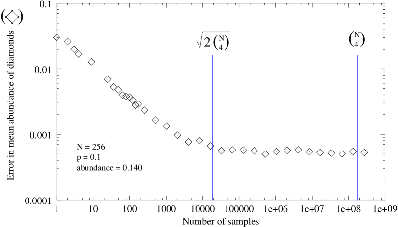
Once one has the mean abundances of all the 4-orders, the mean abundances of the smaller causets can be found by further coarse graining. By explicitly carrying out this coarse graining, one easily deduces the following relationships:

$$f_{3}(\,\,\begin{picture}(0.0,2.0)\put(0.0,0.0){\circle*{0.6}}\put(0.0,1.0){\circle*{0.6}}\put(0.0,2.0){\circle*{0.6}} \put(0.0,0.0){\line(0,1){2.0}} \end{picture}\,\,) = f_{4}(\,\,\begin{picture}(0.0,3.0)\put(0.0,0.0){\circle*{0.6}}\put(0.0,1.0){\circle*{0.6}}\put(0.0,2.0){\circle*{0.6}}\put(0.0,3.0){\circle*{0.6}} \put(0.0,0.0){\line(0,1){3.0}} \end{picture}\,\,)+{1\over 2}\left(f_{4}(\,\,\begin{picture}(2.0,2.0)\put(0.0,0.0){\circle*{0.6}}\put(0.0,1.0){\circle*{0.6}}\put(0.0,2.0){\circle*{0.6}} \put(2.0,2.0){\circle*{0.6}} \put(0.0,0.0){\line(0,1){2.0}} \put(0.0,1.0){\line(2,1){2.0}} \end{picture}\,\,)+f_{4}(\,\,\begin{picture}(2.0,2.0)\put(0.0,0.0){\circle*{0.6}}\put(0.0,1.0){\circle*{0.6}}\put(0.0,2.0){\circle*{0.6}} \put(2.0,0.0){\circle*{0.6}} \put(0.0,0.0){\line(0,1){2.0}} \put(0.0,1.0){\line(2,-1){2.0}} \end{picture}\,\,)\right)+\frac{1}{4}f_{4}(\,\,\begin{picture}(1.0,2.0)\put(0.0,0.0){\circle*{0.6}}\put(0.0,1.0){\circle*{0.6}}\put(0.0,2.0){\circle*{0.6}} \put(1.0,0.0){\circle*{0.6}} \put(0.0,0.0){\line(0,1){2.0}} \end{picture}\,\,)+\frac{1}{4}\left(f_{4}(\,\,\begin{picture}(2.0,2.0)\put(0.0,0.0){\circle*{0.6}}\put(0.0,1.0){\circle*{0.6}}\put(0.0,2.0){\circle*{0.6}} \put(2.0,1.0){\circle*{0.6}} \put(0.0,0.0){\line(0,1){2.0}} \put(0.0,0.0){\line(2,1){2.0}} \end{picture}\,\,)+f_{4}(\,\,\begin{picture}(2.0,2.0)\put(0.0,0.0){\circle*{0.6}}\put(0.0,1.0){\circle*{0.6}}\put(0.0,2.0){\circle*{0.6}} \put(2.0,1.0){\circle*{0.6}} \put(0.0,0.0){\line(0,1){2.0}} \put(2.0,1.0){\line(-2,1){2.0}} \end{picture}\,\,)\right)+{1\over 2}f_{4}(\,\,\begin{picture}(2.0,2.0)\put(0.0,0.0){\circle*{0.6}}\put(0.0,1.0){\circle*{0.6}}\put(0.0,2.0){\circle*{0.6}} \put(2.0,1.0){\circle*{0.6}} \put(0.0,0.0){\line(0,1){2.0}} \put(0.0,0.0){\line(2,1){2.0}} \put(2.0,1.0){\line(-2,1){2.0}} \end{picture}\,\,)$$

$$f_{3}(\,\,\begin{picture}(2.0,2.0)\put(1.0,0.0){\circle*{0.6}} \put(0.0,2.0){\circle*{0.6}}\put(2.0,2.0){\circle*{0.6}} \put(1.0,0.0){\line(-1,2){1.0}} \put(1.0,0.0){\line(1,2){1.0}} \end{picture}\,\,) = {1\over 2}\,f_{4}(\,\,\begin{picture}(2.0,2.0)\put(0.0,0.0){\circle*{0.6}}\put(0.0,1.0){\circle*{0.6}}\put(0.0,2.0){\circle*{0.6}} \put(2.0,2.0){\circle*{0.6}} \put(0.0,0.0){\line(0,1){2.0}} \put(0.0,1.0){\line(2,1){2.0}} \end{picture}\,\,)+{1\over 2}f_{4}(\,\,\begin{picture}(2.0,2.0)\put(0.0,0.0){\circle*{0.6}}\put(0.0,1.0){\circle*{0.6}}\put(0.0,2.0){\circle*{0.6}} \put(2.0,1.0){\circle*{0.6}} \put(0.0,0.0){\line(0,1){2.0}} \put(0.0,0.0){\line(2,1){2.0}} \end{picture}\,\,)+\frac{1}{4}f_{4}(\,\,\begin{picture}(2.0,2.0)\put(0.0,0.0){\circle*{0.6}}\put(0.0,1.0){\circle*{0.6}}\put(0.0,2.0){\circle*{0.6}} \put(2.0,1.0){\circle*{0.6}} \put(0.0,0.0){\line(0,1){2.0}} \put(0.0,0.0){\line(2,1){2.0}} \put(2.0,1.0){\line(-2,1){2.0}} \end{picture}\,\,)+\frac{3}{4}f_{4}(\,\,\begin{picture}(2.0,2.0)\put(0.0,2.0){\circle*{0.6}}\put(1.0,2.0){\circle*{0.6}}\put(2.0,2.0){\circle*{0.6}} \put(1.0,0.0){\circle*{0.6}} \put(1.0,0.0){\line(-1,2){1.0}} \put(1.0,0.0){\line(0,1){2.0}} \put(1.0,0.0){\line(1,2){1.0}} \end{picture}\,\,)+\frac{1}{4}f_{4}(\,\begin{picture}(3.0,2.0)\put(0.0,2.0){\circle*{0.6}}\put(2.0,2.0){\circle*{0.6}} \put(1.0,0.0){\circle*{0.6}}\put(3.0,0.0){\circle*{0.6}} \put(1.0,0.0){\line(-1,2){1.0}} \put(1.0,0.0){\line(1,2){1.0}} \end{picture}\,\,)+\frac{1}{4}f_{4}(\,\,\begin{picture}(1.0,2.0)\put(0.0,0.0){\circle*{0.6}}\put(0.0,2.0){\circle*{0.6}} \put(1.0,0.0){\circle*{0.6}}\put(1.0,2.0){\circle*{0.6}} \put(0.0,0.0){\line(0,1){2.0}} \put(1.0,0.0){\line(0,1){2.0}} \put(0.0,0.0){\line(1,2){1.0}} \end{picture}\,\,)+{1\over 2}f_{4}(\,\,\begin{picture}(2.0,2.0)\put(0.0,0.0){\circle*{0.6}}\put(0.0,2.0){\circle*{0.6}} \put(2.0,0.0){\circle*{0.6}}\put(2.0,2.0){\circle*{0.6}} \put(0.0,0.0){\line(0,1){2.0}} \put(2.0,0.0){\line(0,1){2.0}} \put(0.0,0.0){\line(1,1){2.0}} \put(2.0,0.0){\line(-1,1){2.0}} \end{picture}\,\,)$$

$$f_{3}(\,\,\begin{picture}(2.0,2.0)\put(0.0,0.0){\circle*{0.6}}\put(1.5,0.0){\circle*{0.6}} \put(0.0,2.0){\circle*{0.6}} \put(0.0,0.0){\line(0,1){2.0}} \end{picture}\,\,) = \frac{3}{4}f_{4}(\,\,\begin{picture}(1.0,2.0)\put(0.0,0.0){\circle*{0.6}}\put(0.0,1.0){\circle*{0.6}}\put(0.0,2.0){\circle*{0.6}} \put(1.0,0.0){\circle*{0.6}} \put(0.0,0.0){\line(0,1){2.0}} \end{picture}\,\,)+\frac{1}{4}\left(f_{4}(\,\,\begin{picture}(2.0,2.0)\put(0.0,0.0){\circle*{0.6}}\put(0.0,1.0){\circle*{0.6}}\put(0.0,2.0){\circle*{0.6}} \put(2.0,1.0){\circle*{0.6}} \put(0.0,0.0){\line(0,1){2.0}} \put(0.0,0.0){\line(2,1){2.0}} \end{picture}\,\,)+f_{4}(\,\,\begin{picture}(2.0,2.0)\put(0.0,0.0){\circle*{0.6}}\put(0.0,1.0){\circle*{0.6}}\put(0.0,2.0){\circle*{0.6}} \put(2.0,1.0){\circle*{0.6}} \put(0.0,0.0){\line(0,1){2.0}} \put(2.0,1.0){\line(-2,1){2.0}} \end{picture}\,\,)\right)+{1\over 2}\left(f_{4}(\,\begin{picture}(3.0,2.0)\put(0.0,2.0){\circle*{0.6}}\put(2.0,2.0){\circle*{0.6}} \put(1.0,0.0){\circle*{0.6}}\put(3.0,0.0){\circle*{0.6}} \put(1.0,0.0){\line(-1,2){1.0}} \put(1.0,0.0){\line(1,2){1.0}} \end{picture}\,\,)+f_{4}(\,\begin{picture}(3.0,2.0)\put(1.0,2.0){\circle*{0.6}} \put(3.0,0.0){\circle*{0.6}} \put(0.0,0.0){\circle*{0.6}}\put(2.0,0.0){\circle*{0.6}} \put(0.0,0.0){\line(1,2){1.0}} \put(2.0,0.0){\line(-1,2){1.0}} \end{picture}\,\,\,)\right)+f_{4}(\,\,\begin{picture}(1.0,1.0)\put(0.0,0.0){\circle*{0.6}}\put(0.0,1.0){\circle*{0.6}} \put(1.0,0.0){\circle*{0.6}}\put(1.0,1.0){\circle*{0.6}} \put(0.0,0.0){\line(0,1){1.0}} \put(1.0,0.0){\line(0,1){1.0}} \end{picture}\,\,)+{1\over 2}f_{4}(\,\,\begin{picture}(2.0,1.0)\put(0.0,0.0){\circle*{0.6}}\put(1.0,0.0){\circle*{0.6}}\put(2.0,0.0){\circle*{0.6}} \put(0.0,1.0){\circle*{0.6}} \put(0.0,0.0){\line(0,1){1.0}} \end{picture}\,\,)$$

$$+{1\over 2}f_{4}(\,\,\begin{picture}(1.0,2.0)\put(0.0,0.0){\circle*{0.6}}\put(0.0,2.0){\circle*{0.6}} \put(1.0,0.0){\circle*{0.6}}\put(1.0,2.0){\circle*{0.6}} \put(0.0,0.0){\line(0,1){2.0}} \put(1.0,0.0){\line(0,1){2.0}} \put(0.0,0.0){\line(1,2){1.0}} \end{picture}\,\,)$$

$$f_{3}(\,\,\begin{picture}(2.0,2.0)\put(1.0,2.0){\circle*{0.6}} \put(0.0,0.0){\circle*{0.6}}\put(2.0,0.0){\circle*{0.6}} \put(0.0,0.0){\line(1,2){1.0}} \put(2.0,0.0){\line(-1,2){1.0}} \end{picture}\,\,) = {1\over 2}\,f_{4}(\,\,\begin{picture}(2.0,2.0)\put(0.0,0.0){\circle*{0.6}}\put(0.0,1.0){\circle*{0.6}}\put(0.0,2.0){\circle*{0.6}} \put(2.0,0.0){\circle*{0.6}} \put(0.0,0.0){\line(0,1){2.0}} \put(0.0,1.0){\line(2,-1){2.0}} \end{picture}\,\,)+{1\over 2}f_{4}(\,\,\begin{picture}(2.0,2.0)\put(0.0,0.0){\circle*{0.6}}\put(0.0,1.0){\circle*{0.6}}\put(0.0,2.0){\circle*{0.6}} \put(2.0,1.0){\circle*{0.6}} \put(0.0,0.0){\line(0,1){2.0}} \put(2.0,1.0){\line(-2,1){2.0}} \end{picture}\,\,)+\frac{1}{4}f_{4}(\,\,\begin{picture}(2.0,2.0)\put(0.0,0.0){\circle*{0.6}}\put(0.0,1.0){\circle*{0.6}}\put(0.0,2.0){\circle*{0.6}} \put(2.0,1.0){\circle*{0.6}} \put(0.0,0.0){\line(0,1){2.0}} \put(0.0,0.0){\line(2,1){2.0}} \put(2.0,1.0){\line(-2,1){2.0}} \end{picture}\,\,)+\frac{3}{4}f_{4}(\,\,\begin{picture}(2.0,2.0)\put(0.0,0.0){\circle*{0.6}}\put(1.0,0.0){\circle*{0.6}}\put(2.0,0.0){\circle*{0.6}} \put(1.0,2.0){\circle*{0.6}} \put(0.0,0.0){\line(1,2){1.0}} \put(1.0,0.0){\line(0,1){2.0}} \put(2.0,0.0){\line(-1,2){1.0}} \end{picture}\,\,)+\frac{1}{4}f_{4}(\,\begin{picture}(3.0,2.0)\put(1.0,2.0){\circle*{0.6}} \put(3.0,0.0){\circle*{0.6}} \put(0.0,0.0){\circle*{0.6}}\put(2.0,0.0){\circle*{0.6}} \put(0.0,0.0){\line(1,2){1.0}} \put(2.0,0.0){\line(-1,2){1.0}} \end{picture}\,\,\,)+\frac{1}{4}f_{4}(\,\,\begin{picture}(1.0,2.0)\put(0.0,0.0){\circle*{0.6}}\put(0.0,2.0){\circle*{0.6}} \put(1.0,0.0){\circle*{0.6}}\put(1.0,2.0){\circle*{0.6}} \put(0.0,0.0){\line(0,1){2.0}} \put(1.0,0.0){\line(0,1){2.0}} \put(0.0,0.0){\line(1,2){1.0}} \end{picture}\,\,)+{1\over 2}f_{4}(\,\,\begin{picture}(2.0,2.0)\put(0.0,0.0){\circle*{0.6}}\put(0.0,2.0){\circle*{0.6}} \put(2.0,0.0){\circle*{0.6}}\put(2.0,2.0){\circle*{0.6}} \put(0.0,0.0){\line(0,1){2.0}} \put(2.0,0.0){\line(0,1){2.0}} \put(0.0,0.0){\line(1,1){2.0}} \put(2.0,0.0){\line(-1,1){2.0}} \end{picture}\,\,)$$

$$f_{3}(\,\begin{picture}(2.0,1.0)\put(0.0,0.5){\circle*{0.6}}\put(1.0,0.5){\circle*{0.6}}\put(2.0,0.5){\circle*{0.6}} \end{picture}\,\,) = \frac{1}{4}\left(f_{4}(\,\,\begin{picture}(2.0,2.0)\put(0.0,2.0){\circle*{0.6}}\put(1.0,2.0){\circle*{0.6}}\put(2.0,2.0){\circle*{0.6}} \put(1.0,0.0){\circle*{0.6}} \put(1.0,0.0){\line(-1,2){1.0}} \put(1.0,0.0){\line(0,1){2.0}} \put(1.0,0.0){\line(1,2){1.0}} \end{picture}\,\,)+f_{4}(\,\,\begin{picture}(2.0,2.0)\put(0.0,0.0){\circle*{0.6}}\put(1.0,0.0){\circle*{0.6}}\put(2.0,0.0){\circle*{0.6}} \put(1.0,2.0){\circle*{0.6}} \put(0.0,0.0){\line(1,2){1.0}} \put(1.0,0.0){\line(0,1){2.0}} \put(2.0,0.0){\line(-1,2){1.0}} \end{picture}\,\,)\right)+\frac{1}{4}\left(f_{4}(\,\begin{picture}(3.0,2.0)\put(0.0,2.0){\circle*{0.6}}\put(2.0,2.0){\circle*{0.6}} \put(1.0,0.0){\circle*{0.6}}\put(3.0,0.0){\circle*{0.6}} \put(1.0,0.0){\line(-1,2){1.0}} \put(1.0,0.0){\line(1,2){1.0}} \end{picture}\,\,)+f_{4}(\,\begin{picture}(3.0,2.0)\put(1.0,2.0){\circle*{0.6}} \put(3.0,0.0){\circle*{0.6}} \put(0.0,0.0){\circle*{0.6}}\put(2.0,0.0){\circle*{0.6}} \put(0.0,0.0){\line(1,2){1.0}} \put(2.0,0.0){\line(-1,2){1.0}} \end{picture}\,\,\,)\right)+{1\over 2}f_{4}(\,\,\begin{picture}(2.0,1.0)\put(0.0,0.0){\circle*{0.6}}\put(1.0,0.0){\circle*{0.6}}\put(2.0,0.0){\circle*{0.6}} \put(0.0,1.0){\circle*{0.6}} \put(0.0,0.0){\line(0,1){1.0}} \end{picture}\,\,)+f_{4}(\,\,\begin{picture}(3.0,1.0)\put(0.0,0.5){\circle*{0.6}}\put(1.0,0.5){\circle*{0.6}}\put(2.0,0.5){\circle*{0.6}}\put(3.0,0.5){\circle*{0.6}} \end{picture}\,\,)$$

$$f_{2}(\,\,\begin{picture}(0.0,1.0)\put(0.0,0.0){\circle*{0.6}}\put(0.0,1.0){\circle*{0.6}} \put(0.0,0.0){\line(0,1){1.0}} \end{picture}\,\,) = f_{3}(\,\,\begin{picture}(0.0,2.0)\put(0.0,0.0){\circle*{0.6}}\put(0.0,1.0){\circle*{0.6}}\put(0.0,2.0){\circle*{0.6}} \put(0.0,0.0){\line(0,1){2.0}} \end{picture}\,\,)+\frac{2}{3}\left(f_{3}(\,\,\begin{picture}(2.0,2.0)\put(1.0,0.0){\circle*{0.6}} \put(0.0,2.0){\circle*{0.6}}\put(2.0,2.0){\circle*{0.6}} \put(1.0,0.0){\line(-1,2){1.0}} \put(1.0,0.0){\line(1,2){1.0}} \end{picture}\,\,)+f_{3}(\,\,\begin{picture}(2.0,2.0)\put(1.0,2.0){\circle*{0.6}} \put(0.0,0.0){\circle*{0.6}}\put(2.0,0.0){\circle*{0.6}} \put(0.0,0.0){\line(1,2){1.0}} \put(2.0,0.0){\line(-1,2){1.0}} \end{picture}\,\,)\right)+\frac{1}{3}f_{3}(\,\,\begin{picture}(2.0,2.0)\put(0.0,0.0){\circle*{0.6}}\put(1.5,0.0){\circle*{0.6}} \put(0.0,2.0){\circle*{0.6}} \put(0.0,0.0){\line(0,1){2.0}} \end{picture}\,\,)$$

$$f_{2}(\,\begin{picture}(1.0,1.0)\put(0.0,0.5){\circle*{0.6}}\put(1.0,0.5){\circle*{0.6}} \end{picture}\,\,\,) = 1-f_{2}(\,\,\begin{picture}(0.0,1.0)\put(0.0,0.0){\circle*{0.6}}\put(0.0,1.0){\circle*{0.6}} \put(0.0,0.0){\line(0,1){1.0}} \end{picture}\,\,)$$

In the first six equations, the coefficient before each term on the right is the fraction of coarse-grainings of that causet which yield the causet on the left.

Figure 2.8: Flow of the coarse-grained probabilities $f_{m}$ for $m=2$. The 2-chain probability is held at 1/2.

Figure 2.9: Flow of the coarse-grained probabilities $f_{m}$ for $m=3$. The 2-chain probability is held at 1/2.

Figure 2.10: Flow of the coarse-grained probabilities $f_{m}$ for $m=4$. The 2-chain probability is held at 1/2.

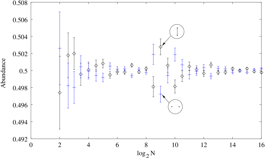
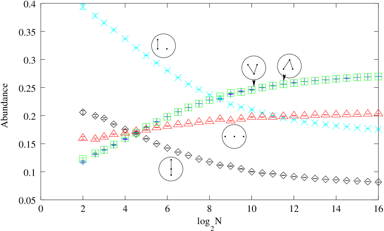
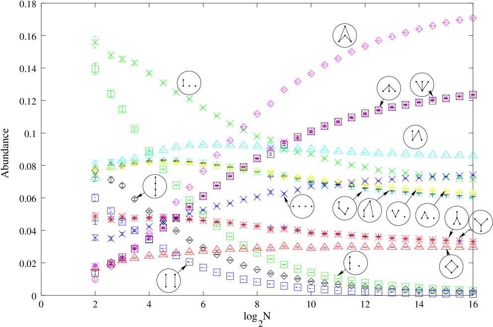
In Figures 2.8, 2.9, and 2.10, we exhibit how the coarse-grained probabilities of all possible 2, 3, and 4 element causets vary as we follow the trajectory along which the coarse-grained 2-chain probability $f_{2}(\,\,\begin{picture}(0.0,1.0)\put(0.0,0.0){\circle*{0.6}}\put(0.0,1.0){\circle*{0.6}} \put(0.0,0.0){\line(0,1){1.0}} \end{picture}\,\,)=r$ is held at $1/2$. By design, the coarse-grained probability for the 2-chain remains flat at 50%, so Figure 2.8 simply shows the accuracy with which this was achieved. (Observe the scale on the vertical axis.) Notice that, since $f_{2}(\,\,\begin{picture}(0.0,1.0)\put(0.0,0.0){\circle*{0.6}}\put(0.0,1.0){\circle*{0.6}} \put(0.0,0.0){\line(0,1){1.0}} \end{picture}\,\,)$ and $f_{2}(\,\begin{picture}(1.0,1.0)\put(0.0,0.5){\circle*{0.6}}\put(1.0,0.5){\circle*{0.6}} \end{picture}\,\,\,)$ must sum to 1, their error bars are necessarily equal. (The standard deviation in the abundances decreases with increasing $N$. The “blip” around $\log_{2}N=9$ occurs simply because I generated fewer causets at that and larger values of $N$ to reduce computational costs.)

The crucial question is whether the probabilities for the three and four element causets tend to definite limits as $N$ tends to infinity. Several features of the diagrams indicate that this is indeed occurring. Most obviously, all the curves, except possibly a couple in Figure 2.10, appear to be leveling off at large $N$. But we can bolster this conclusion by observing in which direction the curves are moving, and considering their interrelationships.

For the moment let us focus our attention on Figure 2.9. A priori there are five coarse-grained probabilities to be followed. That they must add up to unity reduces the degrees of freedom to four. This is reduced further to three by the observation that, due to the time-reversal symmetry of the percolation dynamics, we must have $f_{3}(\,\,\begin{picture}(2.0,2.0)\put(1.0,0.0){\circle*{0.6}} \put(0.0,2.0){\circle*{0.6}}\put(2.0,2.0){\circle*{0.6}} \put(1.0,0.0){\line(-1,2){1.0}} \put(1.0,0.0){\line(1,2){1.0}} \end{picture}\,\,)=f_{3}(\,\,\begin{picture}(2.0,2.0)\put(1.0,2.0){\circle*{0.6}} \put(0.0,0.0){\circle*{0.6}}\put(2.0,0.0){\circle*{0.6}} \put(0.0,0.0){\line(1,2){1.0}} \put(2.0,0.0){\line(-1,2){1.0}} \end{picture}\,\,)$, as duly manifested in their graphs. Moreover, all five of the curves appear to be monotonic, with the curves for     ,      and     rising, and the curves for      and      falling. If we accept this indication of monotonicity from the diagram, then first of all, every probability $f_{3}(\xi)$ must converge to some limiting value, because monotonic bounded functions always do; and some of these limits must be nonzero, because the probabilities must add up to 1. Indeed, since $f_{3}(\,\,\begin{picture}(2.0,2.0)\put(1.0,0.0){\circle*{0.6}} \put(0.0,2.0){\circle*{0.6}}\put(2.0,2.0){\circle*{0.6}} \put(1.0,0.0){\line(-1,2){1.0}} \put(1.0,0.0){\line(1,2){1.0}} \end{picture}\,\,)$ and $f_{3}(\,\,\begin{picture}(2.0,2.0)\put(1.0,2.0){\circle*{0.6}} \put(0.0,0.0){\circle*{0.6}}\put(2.0,0.0){\circle*{0.6}} \put(0.0,0.0){\line(1,2){1.0}} \put(2.0,0.0){\line(-1,2){1.0}} \end{picture}\,\,)$ are rising, they must converge to some nonzero value, and this value must lie below 1/2 in order that the total probability not exceed unity. In consequence, the rising curve $f_{3}(\,\begin{picture}(2.0,1.0)\put(0.0,0.5){\circle*{0.6}}\put(1.0,0.5){\circle*{0.6}}\put(2.0,0.5){\circle*{0.6}} \end{picture}\,\,)$ must also converge to a nontrivial probability (one which is neither 0 nor 1). Taken all in all, then, it looks very much like the $m=3$ coarse-grained theory has a nontrivial $N\rightarrow\infty$ limit, with at least three out of its five probabilities converging to nontrivial values.

Although the “rearrangement” of the coarse-grained probabilities appears much more dramatic in Figure 2.10, similar arguments can be made. Excepting initial “transients”, it seems reasonable to conclude from the data that monotonicity will be maintained. From this, it would follow that the probabilities for      and      (which must be equal by time-reversal symmetry) and the other rising probabilities,     ,     , and     , all approach nontrivial limits. The coarse-graining to 4 elements, therefore, would also admit a continuum limit with a minimum of 4 out of the 11 independent probabilities being nontrivial.

To the extent that the $m=2$ and $m=3$ cases are indicative, then, it is reasonable to conclude that percolation dynamics admits a continuum limit which is non-trivial at all “scales” $m$.

Figure 2.11: Flow of the coarse-grained probabilities $f_{m}$ for $m=2$. The 3-chain probability is held at 0.0814837.

Figure 2.12: Flow of the coarse-grained probabilities $f_{m}$ for $m=3$. The 3-chain probability is held at 0.0814837.

Figure 2.13: Flow of the coarse-grained probabilities $f_{m}$ for $m=4$. The 3-chain probability is held at 0.0814837.

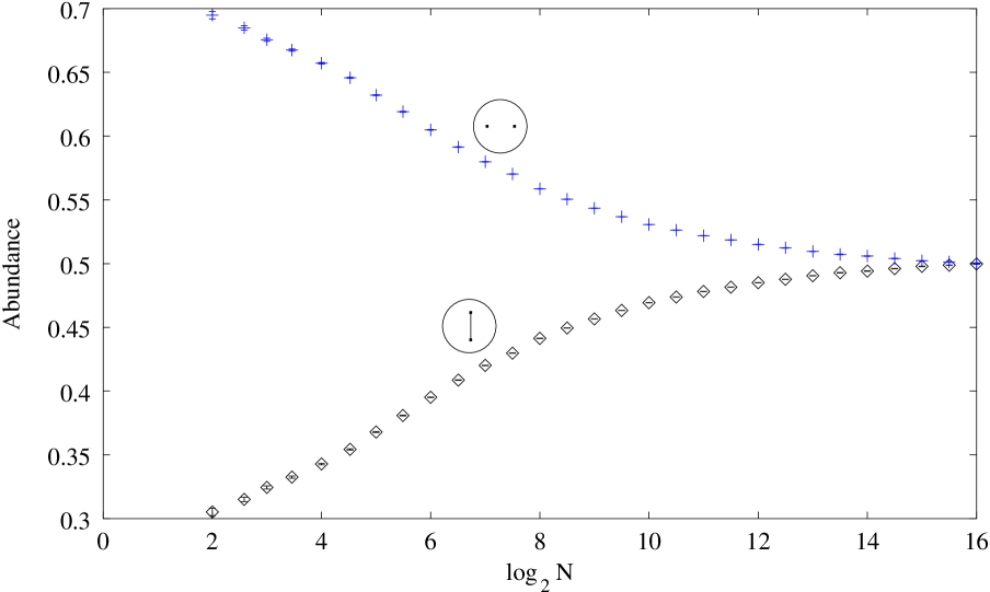
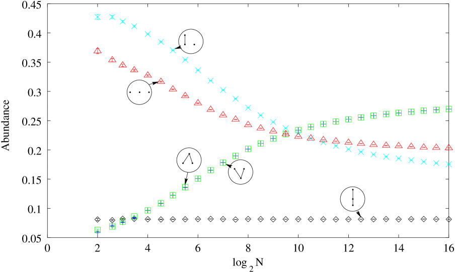
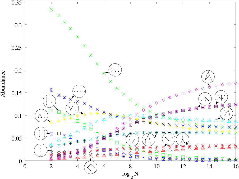
The question suggests itself, whether the flow of the coarse-grained probabilities would differ qualitatively if we held fixed some mean abundance other than that of the 2-chain. In Figures 2.11, 2.12, and 2.13, we display results obtained by fixing the 3-chain abundance (its value having been chosen to make the abundance of 2-chains be 1/2 when $N=2^{16}$). Notice in Figure 2.11 that the abundance of 2-chains varies considerably along this trajectory, whilst that of the 3-chain (in Figure 2.12) of course remains constant. Once again, the figures suggest strongly that the trajectory is approaching a continuum limit with nontrivial values for the coarse-grained probabilities of at least the 3-chain, the “V” and the “$\Lambda$” (and in consequence, of the 2-chain and 2-antichain).

Figure 2.14: Flow of the coarse-grained probabilities $f_{m}$ for $m=3$. The 2-chain probability is held at 1/10.

Figure 2.15: Flow of the coarse-grained probabilities $f_{m}$ for $m=4$. The 2-chain probability is held at 1/10. Only those curves lying high enough to be seen distinctly have been labeled.

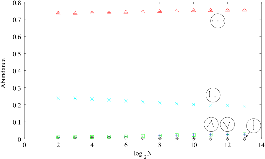
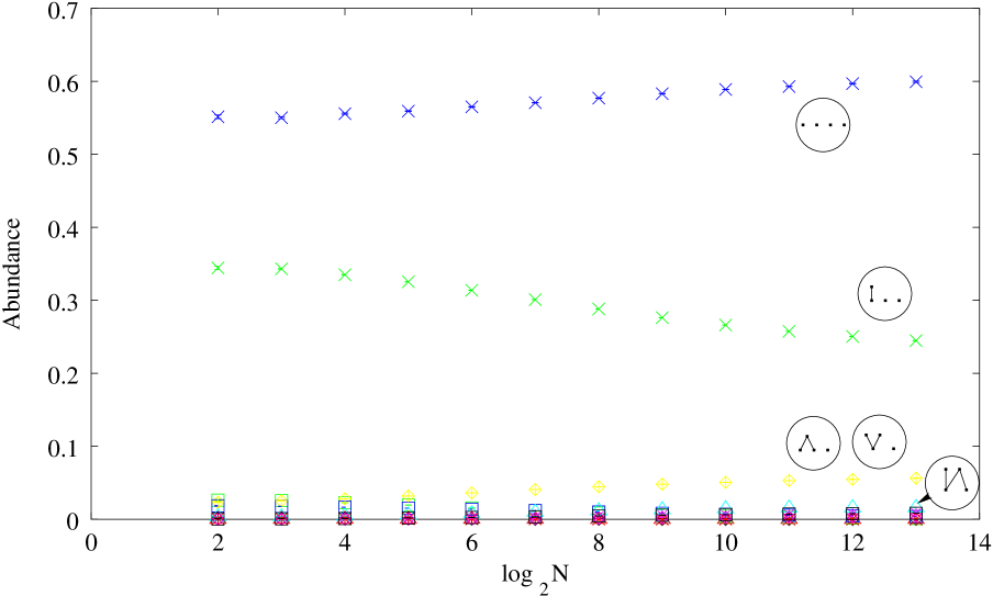
All the trajectories discussed so far produce causets with an ordering fraction $r$ close to 1/2 for large $N$. As mentioned earlier, $r=1/2$ corresponds to a Myrheim-Meyer dimension of two. Figures 2.14 and 2.15 show the results of a simulation along the “four dimensional” trajectory defined by $r=1/10$. (The value $r=1/10$ corresponds to a Myrheim-Meyer dimension of 4.) Here the appearance of the flow is much less elaborate, with the curves arrayed simply in order of increasing ordering fraction,     and      being at the top and      and (imperceptibly)      at the bottom. As before, all the curves are monotone as far as can be seen. Aside from the intrinsic interest of the case $d=4$, these results indicate that our conclusions drawn for $d$ near 2 will hold good for all larger $d$ as well.

Figure 2.16: Flow of the coarse-grained probabilities $f_{m}$ for $m=3$. The 3-chain probability is held at 1/2.

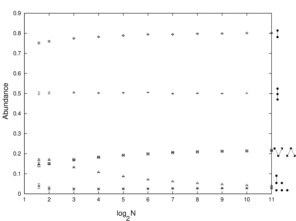
Figure 2.16 displays the flow of the coarse-grained probabilities from a simulation in the opposite situation where the ordering fraction is much greater than 1/2 (the Myrheim-Meyer dimension is down near 1.) Shown are the results of coarse-graining to three element causets along the trajectory which holds the 3-chain probability to 1/2. Also shown is the 2-chain probability. The behavior is similar to that of Figure 2.14, except that here the coarse-grained probability rises with the ordering fraction instead of falling. This occurs because constraining $f_{3}(\,\,\begin{picture}(0.0,2.0)\put(0.0,0.0){\circle*{0.6}}\put(0.0,1.0){\circle*{0.6}}\put(0.0,2.0){\circle*{0.6}} \put(0.0,0.0){\line(0,1){2.0}} \end{picture}\,\,)$ to be 1/2 generates rather chain-like causets whose Myrheim-Meyer dimension is in the neighborhood of 1.34, as follows from the approximate limiting value $f_{2}(\,\,\begin{picture}(0.0,1.0)\put(0.0,0.0){\circle*{0.6}}\put(0.0,1.0){\circle*{0.6}} \put(0.0,0.0){\line(0,1){1.0}} \end{picture}\,\,)\approx 0.8$. The slow, monotonic, variation of the probabilities at large $N$, along with the appearance of convergence to non-zero values in each case, suggests the presence of a nontrivial continuum limit for $r$ near unity as well.

Figure 2.17: Flow of the coarse-grained probabilities $f_{m}$($m-$chain) for $m=2$ to $7$. The 5-chain probability is held at 1/2.

Figure 2.18: Flow of the coarse-grained probabilities $f_{m}$ for $m=4$. The 5-chain probability is held at 1/2.

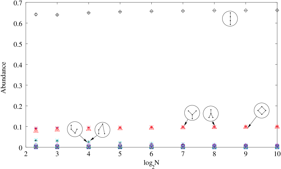
Figures 2.17 and 2.18 present the results of a final set of simulations, the only ones we have carried out which examined the abundances of causets containing more than four elements. In these simulations, the mean 5-chain abundance $f_{5}(\hbox{\rm 5-chain})$ was held at 1/2, producing causets that were even more chain-like than before (Myrheim-Meyer dimension $\approx 1.1$). In Figure 2.17, we track the resulting abundances of all $k$-chains for $k$ between 2 and 7, inclusive. (We limited ourselves to chains, because their abundances are relatively easy to determine computationally.) As in Figure 2.16, all the coarse-grained probabilities appear to be tending monotonically to limits at large $N$. In fact, they look amazingly constant over the whole range of $N$, from 5 to $2^{15}$. One may also observe that the coarse-grained probability of a chain decreases markedly (and almost linearly over the range examined!) with its length, as one might expect. It appears also that the $k$-chain curves for $k\not=5$ are “expanding away” from the 5-chain curve, but only very slightly. Figure 2.18 displays the flow of the probabilities for coarse-grainings to four elements. It is qualitatively similar to Figures 2.14–2.16, with very flat probability curves, and here with a strong preference for causets having many relations over those having few. Comparing Figures 2.18 and 2.15 with Figures 2.13 and 2.10, we observe that trajectories which generate causets that are rather chain-like or antichain-like seem to produce distributions that converge more rapidly than those along which the ordering fraction takes values close to 1/2.

In the way of further simulations, it would be extremely interesting to look for continuum limits of some of the more general dynamical laws discussed in §3.3.5. In doing so, however, one would no longer have available (as one does have for transitive percolation) a very fast (yet easily coded) algorithm that generates causets randomly in accord with the underlying dynamical law. Since the sequential growth dynamics of Chapter 3 is produced by a stochastic process defined recursively on the causal set, it is easily mimicked algorithmically; but the most obvious algorithms that do so are too slow to generate efficiently causets of the size we have discussed in this paper. Hence, one would either have to devise better algorithms for generating causets “one off”, or one would have to use an entirely different method to obtain the mean abundances, like Monte Carlo simulation of the random causet.

2.3.4 Concluding Comments

Transitive percolation is a discrete dynamical theory characterized by a single parameter $p$ lying between $0$ and $1$. Regarded as a stochastic process as described in §3.1.1, it describes the steady growth of a causal set by the continual birth or “accretion” of new elements. If we limit ourselves to that portion of the causet comprising the elements born between step $N_{0}$ and step $N_{1}$ of the stochastic process, we obtain a model of random posets containing $N=N_{1}-N_{0}$ elements.

Because the underlying process is homogeneous, this model does not depend on $N_{0}$ or $N_{1}$ separately, but only on their difference. It is therefore characterized by just two parameters $p$ and $N$. One should be aware that this truncation to a finite model is not consistent with discrete general covariance (c.f. §3.2.2 and §1.3.1), because it is the subset of elements with certain labels that has been selected out of the larger causet, rather than a subset characterized by any directly physical condition. Thus, we have introduced an “element of gauge” and we hope that we are justified in having neglected it. That is, we hope that the random causets produced by the model we have actually studied are representative of the type of suborder that one would obtain by percolating a much larger (eventually infinite) causet and then using a label-invariant criterion to select a subset of $N$ elements.

Leaving this question aside, let us imagine that our model represents an interval (say) in a causet $C$ underlying some macroscopic spacetime manifold. With this image in mind, it is natural to interpret a continuum limit as one in which $N\rightarrow\infty$ while the coarse-grained features of the interval in question remain constant. We have made this notion precise by defining coarse-graining as random selection of a suborder whose cardinality $m$ measures the “coarseness” of our approximation. A continuum limit then is defined to be one in which $N$ tends to $\infty$ such that, for each finite $m$, the induced probability distribution $f_{m}$ on the set of $m$-element posets converges to a definite limit, the physical meaning being that the dynamics at the corresponding length-scale is well defined. Now, how could our model fail to admit such a limit?

In a field-theoretic setting, failure of a continuum limit to exist typically means that the coarse-grained theory loses parameters as the cutoff length goes to zero. For example, $\lambda\phi^{4}$ scalar field theory in 4 dimensions depends on two parameters, the mass $\mu$ and the coupling constant $\lambda$. In the continuum limit, $\lambda$ is lost (i.e. it necessarily vanishes, because it is driven to infinity at finite cutoff if one tries to hold its renormalized value fixed), although one can arrange for $\mu$ to survive. (At least this is what most workers believe occurs.) Strictly speaking, one should not say that a continuum limit fails to exist altogether, but only that the limiting theory is poorer in coupling constants than it was before the limit was taken. Now in our case, we have only one parameter to start with, and we have seen that it does survive as $N\rightarrow\infty$ since we can, for example, choose freely the $m=2$ coarse-grained probability distribution $f_{2}$. Hence, we need not fear such a loss of parameters in our case.

What about the opposite possibility? Could the coarse-grained theory gain parameters in the $N\rightarrow\infty$ limit, as might occur if the distributions $f_{m}$ were sensitive to the fine details of the trajectory along which $N$ and $p$ approached the “critical point” $p=0$, $N=\infty$? Our simulations showed no sign of such sensitivity, although we did not look for it specifically. (Compare, for example, Figure 2.9 with Figure 2.12 and 2.10 with 2.13.)

A third way the continuum limit could fail might perhaps be viewed as an extreme form of the second. It might happen that, no matter how one chose the trajectory $p=p(N)$, some of the coarse-grained probabilities $f_{m}(\xi)$ oscillated indefinitely as $N\rightarrow\infty$, without ever settling down to fixed values. Our simulations leave little room for this kind of breakdown, since they manifest the exact opposite kind of behavior, namely monotone variation of all the coarse-grained probabilities we “measured”.

Finally, a continuum limit could exist in the technical sense, but it still could be effectively trivial (once again reminiscent of the $\lambda\phi^{4}$ case — if you care to regard a free field theory as trivial). Here triviality would mean that all — or almost all — of the coarse-grained probabilities $f_{m}(\xi)$ converged either to 0 or to 1. Plainly, we can avoid this for at least some of the $f_{m}(\xi)$. For example, we could choose an $m$ and hold either $f_{m}(m\hbox{-chain})$ or $f_{m}(m\hbox{-antichain})$ fixed at any desired value. (As $p\rightarrow 1$, $f_{m}(m\hbox{-chain})\rightarrow 1$ and $f_{m}(m\hbox{-antichain})\rightarrow 0$; as $p\rightarrow 0$, the opposite occurs.) However, in principle, it could still happen that all the other $f_{m}$ besides these two went to 0 in the limit. (Clearly, they could not go to 1, the other trivial value.) Once again, our simulations show the opposite behavior. For example, we saw that $f_{3}(\,\,\begin{picture}(2.0,2.0)\put(1.0,0.0){\circle*{0.6}} \put(0.0,2.0){\circle*{0.6}}\put(2.0,2.0){\circle*{0.6}} \put(1.0,0.0){\line(-1,2){1.0}} \put(1.0,0.0){\line(1,2){1.0}} \end{picture}\,\,)$ increased monotonically along the trajectory of Figure 2.9.

Moreover, even without reference to the simulations, we can make this hypothetical “chain-antichain degeneracy” appear very implausible by considering a “typical” causet $C$ generated by percolation for $N\gg 1$ with $p$ on the trajectory that, for some chosen $m$, holds $f_{m}(m\hbox{-chain})$ fixed at a value $a$ strictly between 0 and 1. Then our degeneracy would insist that $f_{m}(m\hbox{-antichain})=1-a$ and $f_{m}(\chi)=0$ for all other $\chi$. But this would mean that, in a manner of speaking, “every” coarse-graining of $C$ to $m$ elements would be either a chain or an antichain. In particular the causet     could not occur as a subcauset of $C$; whence, since     is a subcauset of every $m$-element causet except the chain and the antichain, $C$ itself would have to be either an antichain or a chain. But it is absurd that percolation for any parameter value $p$ other than 0 and 1 would produce a “bimodal” distribution such that $C$ would have to be either a chain or an antichain, but nothing in between. It seems likely that similar arguments could be devised against the possibility of similar, but slightly less trivial trivial continuum limits, for example a limit in which $f_{m}(\chi)$ would vanish unless $\chi$ were a disjoint union of chains and antichains.

Putting all this together, we have persuasive evidence that the percolation model does admit a continuum limit, with the limiting model being nontrivial and described by a single “renormalized” parameter or “coupling constant”. Furthermore, the associated scaling behavior one might think to find in such a case is also present, as will be discussed further in [48].

However, the question remains as to whether this continuum resembles a spacetime manifold, or is something more pathological. Do the causal sets yielded by the percolation dynamics resemble genuine spacetimes? Based on the meager evidence available at the present time, for example that mentioned in §2.2.1 and §2.2.2 we can only answer “it is possible”.

Finally, there is the ubiquitous issue of “fine tuning” or “large numbers”. In any continuum situation, a large number is being manifested (an actual infinity in the case of a true continuum) and one may wonder where it came from. In our case, the large numbers were $p^{-1}$ and $N$. For $N$, there is no mystery: unless the causal set “ends” at some point, $N$ is guaranteed to be as large as desired. But why should $p$ be so small? Here we can appeal to the preliminary results of Dou mentioned in §2.2.7, which state that under cosmological renormalization, certain physically reasonable dynamics of causal sets are driven toward an effective percolation-like phase with a value of $p$ that scales like $N_{0}^{-1/2}$, where $N_{0}$ is the number of elements of the causet preceding the most recent “bounce”. Since this is sure to be an enormous number if one waits long enough, $p$ is sure to become arbitrarily small if sufficiently many cycles occur. The reason for the near flatness of spacetime — or if you like for the large diameter of the contemporary universe — would then be just that the underlying causal set is very old — old enough to have accumulated, let us say, $10^{480}$ elements in earlier cycles of expansion, contraction and re-expansion.

2.4 Scaling

The trajectories of Figure 2.5 can be fit numerically to explore the scaling behavior of this model. Doing so seems to suggest an asymptotic functional form of $\log N/N$, which agrees with the prediction of [45]. Not only does this evidence for scaling support the conclusion of the existence of a continuum limit, but the asymptotic form can also be used to suggest a choice for the parameters $t_{n}$ of the classical dynamics (of (3.21), say) which may produce spacetimes with a dimension which is constant over many length scales. Details will appear in [48].

Chapter 3 Classical Dynamics of Sequential Growth

3.1 Introduction

As illustrated in Chapter 1, the causal set approach to quantum gravity has experienced considerable progress in its kinematic aspects. For example, there exist natural extensions of the concepts of proper time and spacetime dimensionality, which take us a significant way toward an answer to the question, “When does a causal set resemble a Lorentzian manifold?”. The dynamics of causal sets (the “equations of motion”), however, has not been very developed to date. One of the primary difficulties in formulating a dynamics for causal sets is the sparseness of the fundamental mathematical structure. When all one has to work with is a discrete set and a partial order, even the notion of what we should mean by a dynamics is not obvious.

Traditionally, one prescribes a dynamical law by specifying a Hamiltonian to be the generator of the time evolution. This practice presupposes the existence of a continuous time variable, which we do not have in the case of causal sets. Thus, one must conceive of dynamics in a more general sense. Considerable progress can be made by envisaging evolution as a process of stochastic growth to be described in terms of the probabilities (in the classical case, or more generally the quantum measures in the quantum case [56]) of forming designated causal sets. As mentioned in §1.3.1, the dynamical law will be a rule which assigns probabilities to suitable classes of causal sets (a causal set being the “history” of the theory in the sense of “sum-over-histories”). One can then use this rule — technically a probability measure — to ask physically meaningful questions of the theory. For example one could ask “What is the probability that the universe possesses the diamond poset as a partial stem?”.

Why are we interested in a classical dynamics for causal sets, when our ultimate aim is a quantum theory of gravity? One obvious reason is that the classical case, being much simpler, can help us to get used to a relatively unfamiliar type of dynamical formulation, bringing out the pertinent physical issues and guiding us toward physically suitable conditions to place on the theory. Is there, for example, an appropriate form of causality that we can impose? Should we attempt to express the theory directly in terms of gauge invariant (labeling independent) quantities, or should we follow precedent by enforcing gauge invariance only at the end? Some of these issues are well illustrated with the theories we construct herein.

One of the best reasons to be interested in a classical dynamics for causal sets is that quantum gravity must possess general relativity as a classical limit. Thus general relativity should be described as some type of effective classical dynamics for causal sets, and one may hope that the relevant dynamical law will be among the family delineated here. (One can’t be certain this will occur, because general relativity, as a continuum theory, seems most likely to arise as an effective theory for coarse-grained causal sets, rather than directly as a limit of the microscopic discrete theory, and there is no guarantee that this effective theory will have the same form as the underlying exact one.)

A question commonly asked of the causal set program is “How could nongravitational matter arise from only a partial order?”. One obvious answer is that matter can emerge as a higher level construct via the Kaluza-Klein mechanism [29], but this possibility has nothing to do with causal sets as such. The theory developed in this chapter suggests a different mechanism, in that is possible to rewrite the theory in such a way that the dynamics appears to arise from a kind of “effective action” for a field of Ising spins living on the relations of the causal set. A form of “Ising matter” is thus implicit in what would seem at first sight to be a purely “source-free” theory.

3.1.1 Sequential growth

The dynamics which we will derive can be regarded as a process of “cosmological accretion” or “growth”. At each step of this process an element of the causal set comes into being as the “offspring” of a definite set of the existing elements – the elements that form its past. The phenomenological passage of time is taken to be a manifestation of this continuing growth of the causet. Thus, we do not think of the process as happening “in time” but rather as “constituting time”, which means in a practical sense that there is no meaningful order of birth of the elements other than that implied by the relation $\prec$.

In order to define the dynamics, however, we will treat the births as if they happened in a definite order with respect to some fictitious “external time”. In this way, we introduce an element of “gauge” into the description of the growth process which we will have to compensate by imposing appropriate conditions of “gauge invariance”. This fictitious order of birth can be represented as a natural labeling of the elements, that is, a labeling by integers $0,1,2,3,\ldots$ which are compatible with the causal order (recall definition of natural labeling in §1.3.1). The relevant notion of gauge invariance (which we will call “discrete general covariance”) is then captured by the statement that the labels carry no physical meaning. We discuss this more extensively later on.

It is helpful to visualize the growth of the causal set in terms of paths in a poset ${\cal P}$ of finite causal sets. (Thus viewed, the growth process will be a sort of Markov process taking place in ${\cal P}$.) Each finite causet (or rather each isomorphism equivalence class of finite causets) is one element of this poset. If a causet can be formed by accreting a single element to a second causet, then the former (the “child”) follows the latter (the “parent”) in ${\cal P}$ and the relation between them is a link. Drawing ${\cal P}$ as a Hasse diagram of Hasse diagrams, we get Fig. 3.1. (Of course this is only a portion of the infinite diagram; it includes all the causal sets of fewer than five elements and 8 of the 63 five element causets.

Figure 3.1: The poset of finite causets

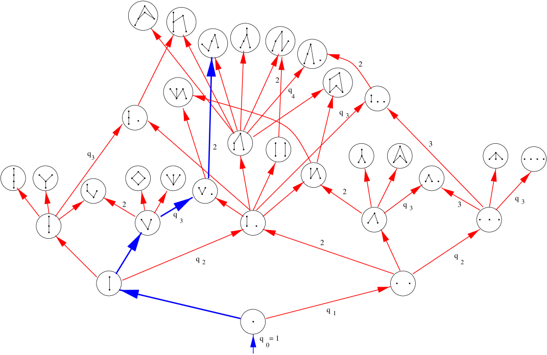
The “decorations” on some of the transitions in Fig. 3.1 are for later use.) Any natural labeling of a causet $C\in{\cal P}$ determines uniquely a path in ${\cal P}$ beginning at the empty causet and ending at $C$. Conversely, any choice of upward path through this diagram determines a naturally labeled causet, or rather a set of them, since inequivalent labelings can sometimes give rise to the same path in ${\cal P}$. We want the physics to be independent of labeling, so different paths in ${\cal P}$ leading to the same causet should be regarded as representing the same (partial) universe, the distinction between them being “pure gauge”.

The causal sets which can be formed by adjoining a single maximal element to a given causet will be called collectively a family. The causet from which they come is their parent, and they are siblings of each other. Each one is a child of the parent. The child formed by adjoining an element which is to the future of every element of the parent will be called the timid child. The child formed by adjoining an element which is spacelike to every other element will be called the gregarious child. A child which is not the timid child will be called a bold child. (At times I may not be careful to distinguish between a child and the transition probability leading to that child, assuming that the intended meaning is obvious from context.)

Each parent-child relationship in ${\cal P}$ describes a ‘transition’ $C\rightarrow C^{\prime}$, from one causal set to another induced by the birth of a new element. The past of the new element (a subset of $C$) will be referred to as the precursor set of the transition (or sometimes just the “precursor of the transition”). Normally, this precursor set is uniquely determined up to automorphism of the parent by the (isomorphism equivalence class of the) child, but (rather remarkably) this is not always the case.

Figure 3.2: Inequivalent precursors lead to same child

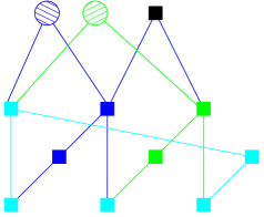
The symbol $\mathcal{C}_{n}$ will denote the set of causets with $n$ elements, and the set of all transitions from $\mathcal{C}_{n}$ to $\mathcal{C}_{n+1}$ will be called stage $n$.

As just remarked, each parent-child transition corresponds to a choice of partial stem in the parent (the precursor of the transition). Since there is a one-to-one correspondence between partial stems and antichains, a choice of child also corresponds to a choice of (possibly empty) antichain in the parent, the antichain in question being the set of maximal elements of the precursor. Note also that the new element will be linked to each element of this antichain.

3.1.2 Some examples

To help clarify the terminology introduced in the previous section, we give some examples. The 20 element causet of Figure 3.3 was generated by the stochastic dynamics described herein, with the choice of parameters given by Equation (3.19) below (with $t=1$).

Figure 3.3: An example of a (‘typical’?) 20 element causal set

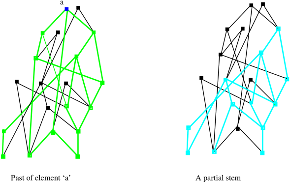
In the copy of this causet on the left, the past of element $a$ is highlighted. Notice that since we use the irreflexive convention for the order, $a$ is not included in its own past. In the the copy on the right, a partial stem of the causet is highlighted.

Figure 3.4 shows     and its children.

Figure 3.4: A family

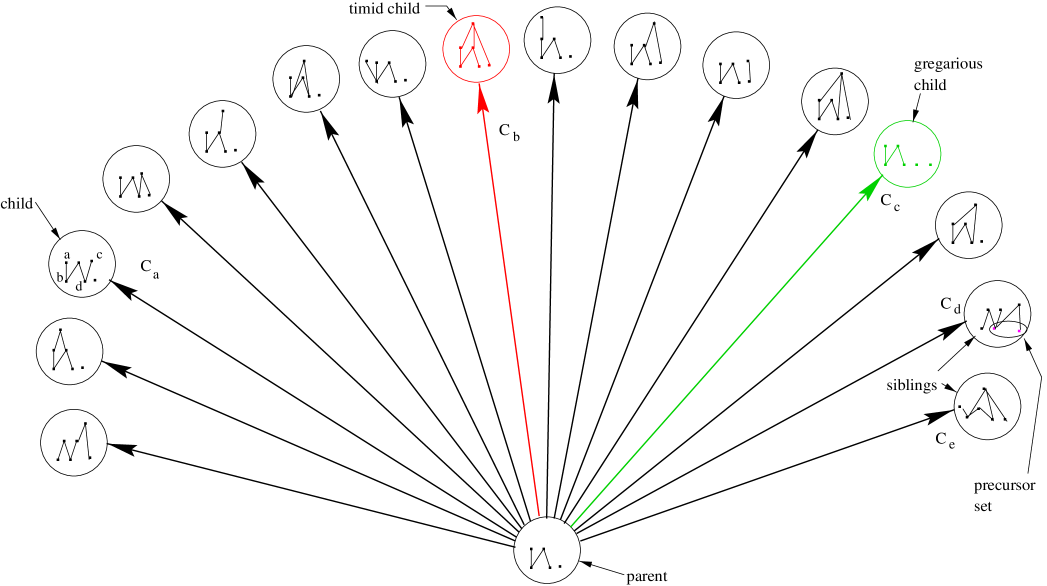
The timid child is $C_{b}$ and the gregarious child is $C_{c}$. The precursor set leading to the transition to $C_{d}$ is shown in the ellipse. An example of an automorphism of $C_{a}$ is the map $a\leftrightarrow c,b\leftrightarrow d$ (the other elements remaining unchanged).

3.2 Physical requirements on the dynamics

The dynamics of transitive percolation, which was introduced in §2.1, can be expressed as a growth dynamics of the sort presented in the previous section, by stating that each new element forges a causal bond independently with each existing element with probability $p\in[0,1]$. (Any causal relation implied by transitivity must then be added in as well.) However, this is only one special case drawn from a much larger universe of possibilities. As preparation for describing these more general possible dynamical rules, let us consider the growth-sequence of a causal set universe.

First element ‘0’ appears (say with probability one, since the universe exists). Then element ‘1’ appears, either related to ‘0’ or not. Then element ‘2’ appears, either related to ‘0’ or ‘1’, or both, or neither. Of course if $1\succ 0$ and $2\succ 1$ then $2\succ 0$ by transitivity. Then element ‘3’ appears with some consistent set of ancestors, and so on and so forth. Because of transitivity, each new element ends up with a partial stem of the previous causet as its precursor set. The result of this process, obviously, is a naturally labeled causet (finite if we stop at some finite stage, or infinite if we do not) whose labels record the order of succession of the individual births. For illustration, consider the path in fig. 3.1 delineated by the heavy arrows. Along this path, element ‘0’ appears initially, then element ‘1’ appears to the future of element ‘0’, then element ‘2’ appears to the future of element ‘0’, but not to the future of ‘1’, then element ‘3’ appears unrelated to any existing element, then element ‘4’ appears to the future of elements ‘0’, ‘1’ (say, or ‘2’, it doesn’t matter) and ‘3’, then element ‘5’ appears (not shown in the diagram), etc.

Let us emphasize once more that the labels 0, 1, 2, etc. are not supposed to be physically significant. Rather, the “external time” that they record is just a way to conceptualize the process, and any two birth sequences related to each other by a permutation of their labels are to be regarded as physically identical.

So far, we have been describing the kinematics of sequential growth. In order to define a dynamics for it, we may give, for each $n$-element causet $C$, the transition probability from it to each of its possible children. Equivalently, we give a transition probability for each partial stem within $C$. We wish to construct a general theory for these transition probabilities by subjecting them to certain natural conditions. In other words, we want to construct the most general (classically stochastic) “sequential growth dynamics” for causal sets. In stating the following conditions, we will employ the terminology introduced above.

3.2.1 The condition of internal temporality

By this imposing sounding phrase, we mean simply that each element is born either to the future of, or unrelated to, all existing elements; that is, no element can arise to the past of an existing element.

We have already assumed this tacitly in describing what we mean by a sequential growth dynamics. An equivalent formulation is that the labeling induced by the order of birth must be natural, as defined above. The logic behind the requirement of internal temporality is that all physical time is that of the intrinsic order defining the causal set itself. For an element to be born to the past of another would be contradictory: it would mean that an event occurred “before” another which intrinsically preceded it.

3.2.2 The condition of discrete general covariance

As we have been emphasizing, the “external time” in which the causal set grows (equivalently the induced labeling of the resulting poset) is not meant to carry any physical information. We interpret this in the present context as being the condition that the net probability of forming any particular $n$-element causet $C$ is independent of the order of birth we attribute to its elements. Thus, if $\gamma$ is any path through the poset ${\cal P}$ of finite causal sets that originates at the empty causet and terminates at $C$, then the product of the transition probabilities along the links of $\gamma$ must be the same as for any other path arriving at $C$. (So general covariance in this setting is a type of path independence). We should recall here, however, that, as observed earlier, a link in ${\cal P}$ can sometimes represent more than one possible transition. Thus our statement of path-independence, to be technically correct, should say that the answer is the same no matter which transition (partial stem) we select to represent the link. Obviously, this immediately entails that all such representatives share the same transition probability.

We might with justice have required here conditions that are apparently much stronger, including the condition that any two paths through ${\cal P}$ with the same initial and final endpoints have the same product of transition probabilities. However, it is easy to see that this already follows from the condition stated. We therefore do not make it part of our definition of discrete general covariance, although we will be using it crucially.

Finally, it is well to remark here that just because the “arrival probability at $C$” is independent of path/labeling, that does not necessarily mean that it carries an invariant meaning. On the contrary a statement like “when the causet had 8 elements it was a chain” is itself meaningless before a certain birth order is chosen. This, also, is an aspect of the gauge problem, but not one that functions as a constraint on the transition probabilities that define our dynamics. Rather it limits the physically meaningful questions that we can ask of the dynamics. Technically, we expect that our dynamics (like any stochastic process) can be interpreted as a probability measure on a certain $\sigma$-algebra, and the requirement of general covariance will, in addition providing a constraint on the transition probabilities of the growth process, serve to select the subalgebra of sets whose measures have direct physical meaning.

3.2.3 The Bell causality condition

The condition of “internal temporality” may be viewed as a very weak type of causality condition. The further causality condition we introduce now is a discrete analog of the statement that no influence can propagate faster than light. This condition is quite strong, being similar to that from which one derives Bell’s inequalities. We believe that such a condition is appropriate for a classical theory, and we expect that some analog will be valid in the quantum case as well. (On the other hand, we would have to abandon Bell causality if our aim were to reproduce quantum effects from a classical stochastic dynamics, as is sometimes advocated in the context of “hidden variable theories”. Given the inherent non-locality of causal sets, there is no logical reason why such an attempt would have to fail.)

The physical idea behind our condition is that events occurring in some part of a causal set $C$ should be influenced only by the portion of $C$ lying to their past. In this way, the order relation constituting $C$ will be causal in the dynamical sense, and not only in name. In terms of our sequential growth dynamics, we make this precise as the requirement that the ratio of the transition probabilities leading to two possible children of a given causet depend only on the triad consisting of the two corresponding precursor sets and their union.

Thus, let $C\rightarrow{}C_{1}$ designate a transition from $C\in\mathcal{C}_{n}$ to $C_{1}\in\mathcal{C}_{n+1}$, and similarly for $C\rightarrow{}C_{2}$. Then, the Bell causality condition can be expressed as the equality of two ratios

$$\frac{prob(C\rightarrow C_{1})}{prob(C\rightarrow C_{2})}=\frac{prob(B\rightarrow B_{1})}{prob(B\rightarrow B_{2})}$$ (3.1)

where $B\in\mathcal{C}_{m}$, ${m}\leq{n}$, is the union of the precursor set of $C\rightarrow C_{1}$ with the precursor set of $C\rightarrow C_{2}$, $B_{1}\in\mathcal{C}_{m+1}$ is $B$ with an element added in the same manner as in the transition $C\rightarrow{C_{1}}$, and $B_{2}\in\mathcal{C}_{m+1}$ is $B$ with an element added in the same manner as in the transition $C\rightarrow C_{2}$. (Notice that if the union of the precursor sets is the entire parent causet, then the Bell causality condition reduces to a trivial identity.)

To clarify the relationships among the causets involved, it may help to characterize the latter in yet another way. Let $e_{1}$ be the element born in the transition $C\rightarrow{}C_{1}$ and let $e_{2}$ be the element born in the transition $C\rightarrow{}C_{2}$. Then $C_{i}=C\cup\{e_{i}\}$ ($i=1,2$), and we have $B=(\mathrm{past}\,e_{1})\cup(\mathrm{past}\,e_{2})$ and $B_{i}=B\cup\{e_{i}\}$ ($i=1,2$).

By its definition, Bell causality relates ratios of transition probabilities belonging to one “stage” of the growth process to ratios of transition probabilities belonging to previous stages. For illustration, consider the case depicted in fig. 3.5.

Figure 3.5: Illustrating Bell causality

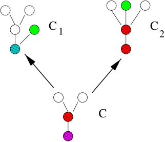
The precursor $P_{1}$ of the transition $C\rightarrow{}C_{1}$ contains only the earliest (minimum) element of $C$, shown in the figure as a pattern-filled dot. The precursor $P_{2}$ of $C\rightarrow{}C_{2}$ contains as well the next earliest element, shown as a (different pattern)-filled dot. The union of the two precursors is thus $B={P_{1}}\cup{P_{2}}=P_{2}$. The elements of $C$ depicted as open dots belong to neither precursor. Such elements will be called spectators. Bell causality says that the spectators can be deleted without affecting relative probabilities. Thus the ratio of the transition probabilities of Figure 3.5 is equal to that of Figure 3.6.

Figure 3.6: Illustrating Bell causality - spectators do not affect relative probability

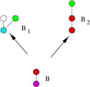
3.2.4 The Markov sum rule

As with any Markov process, we must require that the sum of the full set of transition probabilities issuing from a given causet be unity. However, the set we have to sum over depends in a subtle manner on the extent to which we regard causal set elements as “distinguishable”. Heretofore we have identified distinct transitions with distinct precursor sets of the parent. In doing so, we have in effect been treating causet elements as distinguishable (by not identifying with each other, precursor sets related by automorphisms of the parent), and this is what we shall continue to do. Indeed, this is the counting of children used implicitly by transitive percolation, so we keep it here for consistency. With respect to the diagram of Figure 3.1, this method of counting has the effect of introducing coefficients into the sum rule, equal to the number of partial stems of the parent which could be the precursor set of the transition. For the transitions depicted there, these coefficients (when not one) are shown next to the corresponding arrow.

These sum-rule coefficients admit an alternative description in terms of embeddings of the parent into the child (as a partial stem). Instead of saying “the number of partial stems of the parent which could be the past of the new element”, we could say “the number of order preserving injective maps from the parent onto partial stems of the child, divided by the number of automorphisms of the child”. To see this, let $e$ be such an embedding of parent $P$ into child $C$.

$$P\stackrel{{\scriptstyle e}}{{\longrightarrow}}C$$

Given that the child has precisely one more element than the parent, the injective map $e$ singles out an element as the unique member of $C$ not belonging to the image of $e$. This element can be regarded as the new element that arises from the transition $P\rightarrow C$. The past of this element (in $P$), $\Pi(e)$, will then be a possible precursor of this transition

$$\Pi(e)=e^{-1}(\mathrm{past}(C\setminus e(P)))\>.$$ (3.2)

However, the maps $e$ overcount the number of precursors by the number of automorphisms of the child, since each $e$ composed with an automorphism $\alpha\in\mathrm{Aut}(C)$ yields a new map $f=\alpha\circ e$ which corresponds to the same precursor. To prove this, we must show that

$$\Pi(e)=\Pi(f)\Leftrightarrow f=\alpha\circ e$$

To prove $\Leftarrow$, insert (3.2) for $f$

$$\Pi(f) = (\alpha\circ e)^{-1}(\mathrm{past}(C\setminus\alpha(e(P))))$$

$$= (\alpha e)^{-1}(\mathrm{past}(\alpha(C\setminus e(P))))$$

$$= (\alpha e)^{-1}\alpha(\mathrm{past}(C\setminus e(P)))$$

$$= e^{-1}\alpha^{-1}\alpha(\mathrm{past}(C\setminus e(P)))$$

$$= \Pi(e)\>.$$

The third equality holds because $\alpha$ is an automorphism. To prove $\Rightarrow$, write $f$ as $\beta\circ e$, for some map $\beta:C\rightarrow C$. We then have

$$e^{-1}(\mathrm{past}(C\setminus e(P))) = f^{-1}(\mathrm{past}(C\setminus f(P)))$$

$$= e^{-1}\beta^{-1}(\mathrm{past}(C\setminus\beta(e(P))))$$

$$= e^{-1}\beta^{-1}(\mathrm{past}(\beta(C\setminus e(P))))\>.$$

For this last equality to hold in general, $\beta$ must be an automorphism.

3.3 The general form of the transition probabilities

We seek to derive a general prescription which gives, consistent with our requirements, the transition probability from an element of $\mathcal{C}_{n}$ to an element of $\mathcal{C}_{n+1}$. To avoid having to deal with special cases, we will assume throughout that no transition probability vanishes. Thus the solution we find may be termed “generic”, but not absolutely general.

3.3.1 Counting the free parameters

A theory of the sort we are seeking provides a probability for each transition, so without further restriction, it would contain a free parameter for every possible antichain of every possible (finite) causet. We will see, however, that the requirements described above in Section 3.2 drastically limit this freedom.

Lemma 1

There is at most one free parameter per family.

Proof: Consider a parent and its children (the set of possible transitions from the parent). A Bell causality equation will relate any pair of transitions whose union of precursors is not the entire parent causet, since the remaining elements will then be spectators, whose removal provides such a relation. Since the precursor for the gregarious child is empty, the complement of its union with any other partial stem (save that of the timid child, whose precursor is the entire parent) will be non-empty, resulting in a Bell causality equation relating the pair of transition probabilities. Thus every child, except the timid child, participates in a Bell causality equation with the gregarious child. (See also the proof of Lemma 5 in Appendix A.) Since Bell causality equates ratios, all these transitions are determined up to an overall factor. This leaves two free parameters for the family. The Markov sum rule gives another equation, which exhausts itself in determining the probability of the timid child. Hence precisely one free parameter per family remains after Bell causality and the sum rule are imposed. $\Box$

Lemma 2

The probability to add a completely disconnected element (the “gregarious child transition”) depends only on the cardinality of the parent causal set.

Proof:

Figure 3.7: Equality of “gregarious child” transitions

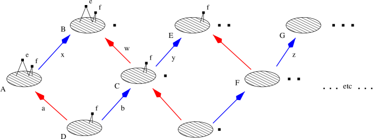
Consider an arbitrary causet $A$, with a maximal element $e$, as indicated in Figure 3.7. Adjoining a disconnected element to $A$ produces the causet $B$. Then, removing $e$ from $B$ leads to the causet $C$, which can be looked upon as the gregarious child of the causet $D=A\backslash\{e\}$. Adding another disconnected element to $C$ leads to a causet $E$ with (at least) two completely disconnected elements. The lower case letter attached to each arrow represents the corresponding transition probability. Now, by general covariance,

$$ax=bw$$

and by Bell causality,

$$\frac{y}{w}=\frac{b}{a}$$

(the disconnected element in $C$ acts as the spectator here). Thus

$$ax=bw=ay\Longrightarrow x=y$$

(Recall that we have assumed that no transition probability vanishes.) Repeating our deductions with $C$ in the place of $A$ in the above argument (and another maximal element $f$ in the place of $e$), we see that $y=z$, where $z$ is the probability for the transition from $F$ to $G$ (which has at least three completely disconnected elements) as shown. Continuing in this way until we reach the antichain $A_{n}$ shows finally that $x=q_{n}$, where we define $q_{n}$ as the transition probability from the $n$-antichain to the ($n+1$)-antichain. Since our starting causet $A$ was not chosen specially, this completes the proof. $\;\;\Box$

If our causal sets are regarded as entire universes, then a gregarious child transition corresponds to the spawning of a new, completely disconnected universe (which is not to say that this new universe will not connect up with the existing universe in the future). Lemma 2 proves that the probability for this to occur does not depend on the internal structure of the existing universe, but only on its size, which seems eminently reasonable. In the sequel, we will call this probability $q_{n}$.

With Lemmas 1 and 2, we have reduced the number of free parameters (since every family has a gregarious child) to 1 per stage, or what is the same thing, to one per causal set element. In the next sections we will see that no further reduction is possible based on our stated conditions. Thus, the transition probabilities $q_{n}$ can be identified as the free parameters or “coupling constants” of the theory. They are, however, restricted further by inequalities that we will derive below.

3.3.2 The general transition probability in closed form

Given the $q_{n}$, the remaining transition probabilities (for the non-gregarious children) are determined by Bell causality and the sum rule, as we have seen. Here we derive an expression in closed form for an arbitrary transition probability in terms of causet invariants and the parameters $q_{n}$.

3.3.2.1 Mathematical form of transition probabilities

We use the following notation:
$\alpha_{n}$ an arbitrary transition probability from $\mathcal{C}_{n}$ to $\mathcal{C}_{n+1}$ $\beta_{n}$ a transition whose precursor set is not the entire parent (‘bold’ transition) $\gamma_{n}$ a transition whose precursor set is the entire parent (‘timid’ transition)

Notice that the subscript $n$ here refers only to the number of elements of the parent causet; it does not exhibit which particular transition of stage $n$ is intended. A more complete notation might provide $\alpha$, $\beta$ and $\gamma$ with further indices to specify both the parent causet and the precursor set within the parent.

We also set $q_{0}\equiv{}1$ by convention.

Lemma 3

Each transition probability $\alpha_{n}$ of stage $n$ has the form

$$q_{n}\sum_{i=0}^{n}{\xi_{i}\frac{1}{q_{i}}}$$ (3.3)

where the $\xi_{i}$ are integers depending on the individual transition in question.

Proof: This is easily seen to be true for stage 1. Assume it is true for stage $n-1$. Consider a non-timid transition probability $\beta_{n}$ of stage $n$. Bell causality gives

$$\frac{\beta_{n}}{q_{n}}=\frac{\alpha_{n-1}}{q_{n-1}}$$ (3.4)

where $\alpha_{n-1}$ is an appropriate transition probability from stage $n-1$. (Bell causality has the property that not all spectators have to be removed in writing the right hand side of the equation. Any partial stem of the subcauset of spectators may be “kept” in selecting which transition probabilities to place on the right hand side.) So by induction

$$\beta_{n}=\alpha_{n-1}\frac{q_{n}}{q_{n-1}}=\sum_{i=0}^{n-1}\xi_{i}\frac{q_{n-1}}{q_{i}}\frac{q_{n}}{q_{n-1}}=\sum_{i=0}^{n-1}\xi_{i}\frac{q_{n}}{q_{i}}.$$ (3.5)

For a timid transition probability $\gamma_{n}$, we use the Markov sum rule:

$$\gamma_{n}=1-\sum_{j}\beta_{nj}$$ (3.6)

where $j$ labels the possible bold transitions (i.e. the set of proper partial stems of the parent). But then, substituting (3.5) yields immediately

$$\gamma_{n}=1-\sum\limits_{j}\sum\limits_{i=0}^{n-1}{\xi_{ji}\over q_{i}}q_{n}=1-\sum\limits_{i=0}^{n-1}{\sum_{j}\xi_{ji}\over q_{i}}q_{n}\,,$$

which we clearly can put into the form (3.3) by taking $\xi_{i}=-\sum_{j}\xi_{ji}$ for $i<n$ and $\xi_{n}=1$. $\Box$

3.3.2.2 Another look at transitive percolation

The transitive percolation model introduced in Chapter 2 is consistent with the four conditions of Section 3.2. To see this, consider an arbitrary causal set $C_{n}$ of size $n$. Recall that, expressed in terms of a sequential growth process, transitive percolation states that at each stage the new element joins to each pre-existing element with probability $p$, with extra relations added to insure transitivity. Then the transition probability $\alpha_{n}$ from $C_{n}$ to a specified causet $C_{n+1}$ of size $n+1$ is given by

$$\alpha_{n}=p^{m}(1-p)^{n-\varpi}$$ (3.7)

where $m$ is the number of maximal elements in the precursor set and $\varpi$ is the size of the entire precursor set. (This becomes clear if one recalls how the precursor set of a newborn element is generated in transitive percolation: first a set of ancestors is selected at random, and then the ancestors implied by transitivity are added. From this, it follows immediately that a given stem $S\subseteq{}C_{n}$ results from the procedure iff (i) every maximal element of $S$ is selected in the first step, and (ii) no element of $C_{n}\backslash{}S$ is selected in the first step.) In particular, we see that the “gregarious transition” will occur with probability $q_{n}=q^{n}$, where $q=1-p$.

Now consider our four conditions. Internal temporality was built in from the outset, as we know. Discrete general covariance is seen to hold upon writing the net probability of a given $C_{n}$ explicitly in terms of causet invariants (writing it in “manifestly covariant form”, c.f. the discussion in §3.5) as

$${\rm Pr}(C_{n})=W(C_{n})\,p^{L}\,q^{{n\choose 2}-R}$$

where $L$ is the number of links in $C_{n}$, $R$ the number of relations, and $W$ the number of (natural) labelings of $C_{n}$. (To see how this arises, note that each of the links in the causal set have to be “put in by hand”, i.e. a link will never enter during the transitive closure stage of the algorithm, so the $L$ links occur with probability $p^{L}$. Furthermore, each of the ${n\choose 2}-R$ non-relations of the causet must have not been “selected” during pre-transitive closure stage of the algorithm, each of which occurs with probability $q=1-p$. Finally, the transitive percolation algorithm generates labeled posets, so any given unlabeled causet $C_{n}$ can arise in $W(C_{n})$ different ways.)

To see that transitive percolation obeys Bell causality, consider an arbitrary parent causet. The transition probability to a given child is exhibited in eq. (3.7). Consider two different children, one with $(m,\varpi)$=($m_{1}$,$\varpi_{1}$) and the other with $(m,\varpi)$=($m_{2}$,$\varpi_{2}$). Bell causality requires that the ratio of their transition probabilities be the same as if the parent were reduced to the union of the precursor sets of the two transitions, i.e. it requires

$$\frac{p^{m_{1}}q^{n-\varpi_{1}}}{p^{m_{2}}q^{n-\varpi_{2}}}=\frac{p^{m_{1}}q^{n^{\prime}-\varpi_{1}}}{p^{m_{2}}q^{n^{\prime}-\varpi_{2}}}$$

where $n^{\prime}$ is the cardinality of the union of the precursor sets of the two transitions. Thus, Bell causality is satisfied by inspection.

Finally, the Markov sum rule is essentially trivial. At each stage of the growth process, a preliminary choice of ancestors is made by a well-defined probabilistic procedure, and each such choice is mapped uniquely onto a choice of partial stem. Thus the induced probabilities of the partial stems sum automatically to unity.

3.3.2.3 The general transition probability

In the previous section we have shown that transitive percolation produces transition probabilities (3.7) consistent with all our conditions. By equating the right hand side of (3.7) to the general form (3.3) of Lemma 3, we can solve for the $\xi_{i}$ and thus obtain the general solution of our conditions:

$$\alpha_{n}=\sum_{i=0}^{n}{\xi_{i}\frac{1}{q_{i}}}\,q_{n}=p^{m}(1-p)^{n-\varpi}=(1-q)^{m}q^{n-\varpi}$$

Expanding the factor $(1-q)^{m}$, and using the fact that $q_{n}=q^{n}$ for transitive percolation, we get

$$\xi_{i}=(-)^{\varpi-i}{m\choose\varpi-i}.$$

So an arbitrary transition probability in the general dynamics is, according to (3.3)

$$\alpha_{n}=\sum_{i=0}^{n}(-)^{\varpi-i}{m\choose\varpi-i}\frac{q_{n}}{q_{i}}.$$

Noting that the binomial coefficients are zero for $\varpi-i\notin\{0..m\}$, and rearranging the indices, we obtain

$$\alpha_{n}=\sum_{k=0}^{m}(-)^{k}{m\choose k}\frac{q_{n}}{q_{\varpi-k}}$$ . (3.8)

This form for the transition probability exhibits its causal nature particularly clearly: except for the overall normalization factor $q_{n}$, $\alpha_{n}$ depends only on invariants of the associated precursor set.

3.3.3 Inequalities

Since the $\alpha_{n}$ are classical probabilities, each must lie between 0 and 1, and this in turn restricts the possible values of the $q_{n}$. Here we show that it suffices to impose only one inequality per stage; all the others (two per child) then follow. More precisely, what we show is that, if $q_{n}>0$ for all $n$, and if $\alpha_{n}\geq{0}$ for the “timid” transition from the $n$-antichain, then all the $\alpha_{n}$ lie in $[0,1]$. This we establish in the following two “Claims”.
Claim   In order that all the transition probabilities $\alpha_{n}$ fall between 0 and 1, it suffices that each timid transition probability be $\geq 0$.
Proof: As described in the proofs of lemmas 1 and 5, each bold transition (of stage $n$) is given (via Bell causality) by

$$\alpha_{n}=\alpha_{m}\frac{q_{n}}{q_{m}}$$

where $m$ is some natural number less than $n$. The $q$’s are positive. So if the probabilities of the previous stages are positive, then the bold probabilities of stage $n$ are also positive. It follows by induction that all but the timid transition probabilities are positive (since $\alpha_{0}=q_{0}=1$ obviously is). But for the timid transition of each family, we have

$$\gamma_{n}=1-\sum_{i}\beta_{i}$$ (3.9)

where each $\beta_{i}$ is positive. If any of the $\beta_{i}$ is greater than one, $\gamma_{n}$ will obviously be negative. Also (3.9) plainly cannot be greater than one. Consequently, if we require that $\gamma_{n}$ be positive, then all transition probabilities in the family will be in $[0,1]$. $\Box$

In a timid transition, the entire parent is the precursor set, so $\varpi=n$. The inequalities constraining each probability of a given family to be in $[0,1]$ therefore reduce to the sole condition

$$\sum_{k=0}^{m}(-)^{k}{m\choose k}\frac{1}{q_{n-k}}\geq 0\,.$$ (3.10)

Claim   The most restrictive inequality of stage $n$ is the one arising from the $n$-antichain, i.e. the one for which $m=n$. All other inequalities of stage $n$ follow from this inequality and the inequalities for smaller $n$.

Proof: Assume that we have, for $m=n$,

$$\sum_{k=0}^{n}(-)^{k}{n\choose k}\frac{1}{q_{n-k}}\geq 0.$$

Add to this the inequality from stage $n-1$,

$$\sum_{k=0}^{n-1}(-)^{k}{n-1\choose k}\frac{1}{q_{n-k-1}}=\sum_{k=0}^{n}(-)^{k-1}{n-1\choose k-1}\frac{1}{q_{n-k}}\geq 0$$

to get

$$\sum_{k=0}^{n-1}(-)^{k}{n-1\choose k}\frac{1}{q_{n-k}}\geq 0.$$

This is the inequality of stage $n$ for $m=n-1$. (We have used the identity ${n\choose k}={n-1\choose k}+{n-1\choose k-1}$.) Adding to it the inequality of stage $n-1$ with $m=n-2$ yields the inequality of stage $n$ for $m=n-2$. Repeating this process will give all the inequalities of stage $n$. $\;\;\Box$

It is helpful to introduce the quantities

$$t_{n}=\sum_{k=0}^{n}(-)^{n-k}{n\choose k}\frac{1}{q_{k}}$$ (3.11)

Obviously, we have $t_{0}=1$ (since $q_{0}=1$), and we have seen that the full set of inequalities restricting the $q_{n}$ will be satisfied iff $t_{n}\geq 0$ for all $n$. (Recall we are assuming $q_{n}>0,\,\forall n$.) Moreover, given the $t_{n}$, we can recover the $q_{n}$ by inverting (3.11):

Lemma 4

$$\frac{1}{q_{n}}=\sum_{k=0}^{n}{n\choose k}t_{k}$$ (3.12)

Proof: This follows immediately from the identity

$$\sum\limits_{k=0}^{n}{n\choose k}(-)^{n-k}{k\choose m}=\delta^{n}_{m}\>,$$

which itself follows from Equations (27) and (28) on the top of pg. 37 of [60]. $\;\;\Box$
Thus, the $t_{n}$ may be treated as free parameters (subject only to $t_{n}\geq{}0$ and $t_{0}=1$), and the $q_{n}$ can then be derived from (3.12). If this is done, the remaining transition probabilities $\alpha_{n}$ can be re-expressed more simply in terms of the $t_{n}$ by inserting (3.12) into (3.8) to get

$$\frac{\alpha_{n}}{q_{n}}=\sum_{l}t_{l}\sum_{k}(-)^{k}{m\choose k}{\varpi-k\choose l}=\sum_{l}t_{l}{\varpi-m\choose\varpi-l}$$

whence

$$\alpha_{n}=\frac{\sum_{l=m}^{\varpi}{\varpi-m\choose\varpi-l}t_{l}}{\sum_{j=0}^{n}{n\choose j}t_{j}}\>.$$ (3.13)

Here, we have used an identity for binomial coefficients that can be found on page 63 of [27]. To express (3.13) more concisely, define

$$\lambda(\varpi,m)=\sum_{l=m}^{\varpi}{\varpi-m\choose\varpi-l}t_{l}$$

Then $q_{n}=\lambda(n,0)^{-1}$ and

$$\alpha_{n}=\frac{\lambda(\varpi,m)}{\lambda(n,0)}$$ (3.14)

In this way, we arrive at the general solution of our inequalities. (Actually, we go slightly beyond our “genericity” assumption that $\alpha_{n}\not=0$ if we allow some of the $t_{n}$ to vanish; but no harm is done thereby.)

Let us conclude this section by noting that (3.12) implies

$$q_{0}\equiv 1\geq q_{1}\geq q_{2}\geq q_{3}\geq\cdots$$ (3.15)

If we think of the $q_{n}$ as the basic parameters or “coupling constants” of our sequential growth dynamics, then it is as if the universe had a free choice of one parameter at each stage of the process. We thus get an “evolving dynamical law”, but the evolution is not absolutely free, since the allowable values of $q_{n}$ at every stage are limited by the choices already made. On the other hand, if we think of the $t_{n}$ as the basic parameters, then the free choice is unencumbered at each stage. However, unlike the $q_{n}$, the $t_{n}$ cannot be identified with any dynamical transition probability. Rather, they can be realized as ratios of two such probabilities, namely as the ratio $x_{n}/q_{n}$, where $x_{n}$ is the transition probability from an antichain of $n$ elements to the timid child of that antichain. (Thus, if we suppose that the evolving causet at the beginning of stage $n$ is an antichain, then $t_{n}$ is the probability that the next element will be born to the future of every element, divided by the probability that the next element will be born to the future of no element.)

3.3.4 Proof that this dynamics obeys the physical requirements

To complete our derivation, we must show that the sequential growth dynamics given by (3.8) or (3.14) obeys the four conditions set out in Section 3.2.

3.3.4.1 Internal temporality

This condition is built into our definition of the growth process.

3.3.4.2 Discrete general covariance

We have to show that the product of the transition probabilities $\alpha_{n}$ associated with a labeling of a fixed finite causet $C$ is independent of the labeling. But this follows immediately from (3.8) [or (3.14)] once we notice that what remains after the overall product

$$\prod\limits_{j=0}^{|C|-1}q_{j}$$

is factored out, is a product over all elements $x\in{C}$ of poset invariants depending only on the structure of $\mathrm{past}(x)$.

3.3.4.3 Bell causality

Bell causality states that the ratio of the transition probabilities for two siblings depends only on the union of their precursors. Looking at (3.8), consider the ratio of two such probabilities $\alpha_{n1}$ and $\alpha_{n2}$. The $q_{n}$ factors will cancel, leading to an expression which depends only on $\varpi_{1}$, $\varpi_{2}$, $m_{1}$, and $m_{2}$. Since these are all determined by the structure of the precursor sets, Bell causality is satisfied.

3.3.4.4 Markov sum rule

The sum rule states that sum of all transition probabilities $\alpha_{n}$ from a given parent $C$ (of cardinality $|C|=n$) is unity. Since a child can be identified with a partial stem of the parent, we can write this condition, in view of (3.14), as

$$\sum_{S}\sum_{l}t_{l}{|S|-m(S)\choose l-m(S)}=\sum_{j}t_{j}{n\choose j}$$ (3.16)

where $S$ ranges over the partial stems of $C$. This must hold for any $t_{l}$, since they may be chosen freely. Reordering the sums and equating like terms yields

$$\forall l,\ \sum_{S}{|S|-m(S)\choose l-m(S)}={n\choose l}\,,$$ (3.17)

an infinite set of identities which must hold if the sum rule is to be satisfied by our dynamics.

The simplest way to see that (3.17) is true is to resort to transitive percolation, for which $t_{l}=t^{l}$ where $t=p/q=p/(1-p)$ (c.f. (3.18) below). In that case we know that the sum rule is satisfied, so by inspection of (3.16), we see that the identity (3.17) must be true.

A more intuitive proof is illustrated well by the case of $l=3$. Group the terms on the left side according to the number of maximal elements:

$$\begin{array}[]{ccccccccr}\sum\limits_{S\,|\,m(S)=0}{|S|-0\choose 3-0}&+&\sum\limits_{S\,|\,m(S)=1}{|S|-1\choose 3-1}&+&\sum\limits_{S\,|\,m(S)=2}{|S|-2\choose 3-2}&+&\sum\limits_{S\,|\,m(S)=3}{|S|-3\choose 3-3}&=&{n\choose 3}\\ 0&+&\sum\limits_{S\,|\,m(S)=1}{|S|-1\choose 2}&+&\sum\limits_{S\,|\,m(S)=2}(|S|-2)&+&\sum\limits_{S\,|\,m(S)=3}1&=&{n\choose 3}\end{array}$$

The first term is zero because the only partial stem with zero maximal elements is empty (i.e. $|S|=0$). The second term is a sum over all partial stems with one maximal element. This is equivalent to a sum over elements, with the element’s inclusive past forming the partial stem. The summand chooses every possible pair of elements to the past of the maximal element. Thus the second term overall counts the 3-element subcausets of $C$ with a single maximal element. There are two possibilities here, the three-chain     and the “lambda”     . The third term sums over partial stems with two maximal elements, which is equivalent to summing over 2 element antichains, the inclusive past of the antichain being the partial stem. The summand then counts the number of elements to the past of the two maximal ones. Thus the third term overall counts the number of three element subcausets with precisely two maximal elements. Again there are two possibilities, the “V”     , and the “L”,     . Finally, the fourth term is a sum over partial stems with three maximal elements, and this can be interpreted as a sum over all three element antichains    . As this example illustrates, then, the left hand side of (3.17) counts the number of $l$ element subcausets of $C$, placing them into “bins” according to the number of maximal elements of the subcauset. Adding together the bin sizes yields the total number of $l$ element subsets of $C$, which of course equals ${n\choose l}$.

3.3.5 Sample cosmologies

The physical consequences of differing choices of the $t_{n}$ remain to be explored. To get an initial feel for this question, we list some simple examples. (Recall our convention that $t_{0}=1$, or equivalently, $q_{0}=1$, where $q_{0}$ is the probability that the universe is born at all.)

• “Dust universe”

  $$t_{0}=1,\ t_{i}=0,\;i\geq 1$$

  This universe is simply an antichain, since, according to (3.12), $q_{n}=1$ for all $n$. An “example” is shown in Figure 3.8.

  

  Figure 3.8: 16 element dust universe

• “Forest universe”

  $$t_{0}=t_{1}=1;\;t_{i}=0,\;i\geq 2$$

  This yields a universe consisting wholly of trees, since (see the next example) $t_{2}=t_{3}=t_{4}=\cdots=0$ implies that no element of the causet can have more than one past link. The particular choice of $t_{1}=1$ has in addition the remarkable property that, as follows easily from (3.14), every allowed transition of stage $n$ has the same probability $1/(n+1)$. Figure 3.9 displays an example.

  

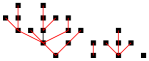
  Figure 3.9: 23 element forest universe

• Case of limited number of past links

  $$t_{i}=0,\;i>n_{0}$$

  Referring to expression (3.14) one sees at once that $\alpha_{n}$ vanishes if $m>n_{0}$. Hence, no element can be born with more than $n_{0}$ past links or “parents”. This means in particular that any realistic choice of parameters will have $t_{n}>0$ for all $n$, since an element of a causal set faithfully embeddable in Minkowski space would have an infinite number of past links. See Figure 3.10 for an example.

  

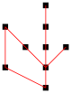
  Figure 3.10: 9 element universe with $t_{1}=t_{2}=1$

• Transitive percolation

  $$t_{n}=t^{n}$$ (3.18)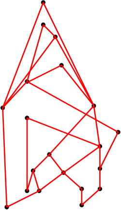

  

  Figure 3.11: 20 element transitive percolation universe with $p=1/4$

  We have seen that for transitive percolation, $q_{n}=q^{n}$, where $q=1-p$. Using the binomial theorem, it is easy to learn from (3.12) or (3.11) that this choice of $q_{n}$ corresponds to $t_{n}=t^{n}$ with $t=p/q$. Clearly, $t$ runs from 0 to $\infty$ as $p$ runs from 0 to 1. Figure 3.11 shows an example.

• A more lifelike choice?

  $$t_{n}=\frac{t^{n}}{n!}$$ (3.19)

  Due to its homogeneity (c.f. §2.2.2), we have seen that transitive percolation with constant $p$ yields causets which could reproduce — at best — only limited portions of Minkowski, de Sitter, or anti-de Sitter space. It also suffers from a sort of “scale dependent dimension” which is incompatible with any continuum spacetime. This occurs because, at finite $p$, transitive percolation generates causets with approximately “constant width” ($\sim 1/p$), meaning that the Hasse diagram looks roughly like an infinite cylinder with cross sectional area of roughly $1/p$. Thus, at larger and larger length scales, the transitive percolation universe looks more and more like a one dimensional spacetime. Both of these issues suggest that one would have to scale $p$ so that it decreased with increasing $n$. This implies that $t_{n}$ should fall off faster than in any percolation model, hence (by the last example) faster than exponentially in $n$. Obviously, there are many possibilities of this sort (e.g. $t_{n}\sim{}e^{-\alpha{}n^{2}}$), but one of the simplest is $t_{n}\sim{c}/n!$. This choice for the $t_{n}$ would be our candidate of the moment for a most physically realistic choice of parameters. (The factor of $t^{n}$ in the numerator, which does not affect the asymptotic behavior, was added by Dou [26], to simplify the study of the cosmological renormalization behavior of this dynamics. In fact, under the renormalization flow, this dynamics approaches that of originary transitive percolation with a $t$ which approaches 0. A 20 element sample causal set “generated by” this dynamics is shown in Figure 3.3.

3.4 Originary dynamics

It is possible that we can arrive at every possible solution of our conditions by taking limits of the generic solution. One such special theory is the originary percolation model, which was introduced in §2.2.5. It is the same as the transitive percolation model, but with the added restriction that each element except the original one must have at least one ancestor among the previous elements. Algorithmically, we generate potential elements one by one, exactly as for plain percolation (by “joining” to each existing element with probability $p$, then adding relations required by transitivity) but discard any such element which would be unrelated to all previous elements. Causets formed with this algorithm always have a single minimal element, an “origin”. The transition probabilities for originary percolation are just those of ordinary transitive percolation with an added factor of $(1-q^{n})$ in the denominator at stage $n$.

This can be generalized to a non-percolation dynamics. Here the causal set grows as usual for a general dynamics, but with the added restriction that it must always possess a 1-chain as a full stem. We call this an originary dynamics. The poset of originary causets can be transformed into the poset of all causets (exactly) by removing the origin from every originary causet.

Further generalizations are also possible, in which a more complex stem of the causet is enforced, e.g. the restriction that after the first two elements form, the causet must always have a 2-chain as a full stem (or partial stem). However, not every poset can be used as a stem in this manner, for many choices are incompatible with Bell causality.

We conjecture that each of these exceptional families of solutions are singular limits of the generic family. For example, originary percolation is the $A\rightarrow\infty$ limit of the dynamics given by $t_{0}=1$, $t_{n}=At^{n}$, $n=1,2,3,\ldots$

3.5 The stochastic growth process as such

We have seen that, associated with every labeled causet $\widehat{C}$ of size $N$, is a net “probability of formation” ${\rm Pr}(\widehat{C})$ which is the product of the transition probabilities $\alpha_{i}$ of the individual births described by the labeling:

$${\rm Pr}(\widehat{C})=\prod\limits_{i=0}^{N-1}\alpha_{i}$$ (3.20)

where $\alpha_{i}=\alpha(i,\varpi_{i},m_{i})$ is given by (3.8) or (3.14), $\varpi_{i}$ and $m_{i}$ are respectively the size and number of maximal elements in the precursor ($\equiv$ past) of the element labeled $i$. Using (3.14), we can write this more explicitly as

$${\rm Pr}(\widehat{C})=\frac{\prod_{i=0}^{N-1}\lambda(\varpi_{i},m_{i})}{\prod_{j=0}^{N-1}\lambda(j,0)}\>.$$ (3.21)

We have also seen that ${\rm Pr}(\widehat{C})$ is in fact independent of the labeling, i.e. ${\rm Pr}(\widehat{C})={\rm Pr}(\breve{C})$ where $\breve{C}$ is the same causet as $\widehat{C}$, but with a different labeling.

The net probability of arriving at an unlabeled causet $C$, at stage $N$ of the growth process is

$${\rm Pr}_{N}(C)=W(C)\,{\rm Pr}(\widehat{C})$$ (3.22)

where $\widehat{C}$ is the causet $C$ endowed with any (natural) labeling, $N=|C|$, and $W(C)$ is the number of inequivalent labelings of $C$, or in other words, the total number of paths through ${\cal P}$ that arrive at $C$, each link being taken with its proper multiplicity. Expressing (3.21) more intrinsically, we can write (3.22) as

$${\rm Pr}_{N}(C)=W(C)\>{\prod\limits_{x\in C}\lambda(\varpi(x),m(x))\over\prod\limits_{j=0}^{|C|-1}\lambda(j,0)}\,,$$ (3.23)

where $\varpi(x)=|\mathrm{past}{x}|$ and $m(x)=|{\rm maximal}(\mathrm{past}x)|$. This expression, as far as it goes, is manifestly “covariant” in the sense explained above. Also causality is manifest in the sense that it is expressed as a product of factors, one for each element (save the $W(C)$), each of which depends only on that element’s past. However, as explained in §3.2.2 and §1.3.1, it has no direct physical meaning. Here we briefly discuss some probabilities which do have a fully covariant meaning and show how, in simple cases, they are related to $N\rightarrow\infty$ limits of probabilities like (3.23).

As a rudimentary example of a truly covariant question, let us take “Does the two-chain ever occur as a partial stem of $C$?”. The answer to this question will be a probability, $P$, which it is natural to identify as

$$P=\lim_{N\rightarrow\infty}{\rm Pr}_{N}(X_{N})\,,$$ (3.24)

where $X_{N}$ is the event that “at stage $N$”, $C$ possesses a partial stem which is a two-chain. To state this more precisely, define $X_{N}$ to be the set of $N$-orders which satisfy some criterion, e.g. that the order possess the causet $S$ as a partial stem ($S$ was a two-chain in the above example), and define

$${\rm Pr}_{N}(X_{N})=\sum_{C\in X_{N}}{\rm Pr}_{N}(C)\>.$$ (3.25)

Of course it is not guaranteed that $P$ will be well defined in the $N\rightarrow\infty$ limit. In this connection, we conjecture that the questions “Does $S$ occur as a partial stem of $C$?” furnish a physically complete set, when $S$ ranges over all (isomorphism equivalence classes of) finite causets.

As a simple example of an answer to a question of this form, consider “What is the probability $P$ that a 1-chain is a full stem of the universe $C$?”. Clearly this is equivalent to the question “Does $C$ have a unique minimal element?”. In terms of partial stems, this question is equivalent to demanding that the 2-antichain not be a partial stem of $C$. The answer is simple to formulate by thinking in terms of the growth process, as follows. At stage 0 of the process, $C$ is a 1-chain, which occurs with probability 1. At stage 1, $C$ must not become a 2-antichain, which occurs with probability $1-q_{1}$. At stage 2, the new element must not be born with no ancestors, which occurs with probability $1-q_{2}$. At stage 3, the same condition occurs with probability $1-q_{3}$, and so on. Thus in the limit $N\rightarrow\infty$, the answer becomes

$$P=\prod_{i=1}^{\infty}(1-q_{i})\;.$$ (3.26)

Expressed in terms of the $t_{n}$, the $q_{i}$ in (3.26) are simply replaced with $1/\sum_{k=0}^{i}{i\choose k}t_{k}$.

3.6 Two Ising-like state-models

The dynamics, as written in (3.20) (say) can be expressed in terms of either of a pair of Ising-like state models. To derive one such model, consider $\alpha_{n}$ as given in (3.8). Inserting this form into (3.20) (and discarding the labeling decoration on $C$)

$${\rm Pr}(C)=\prod_{j=0}^{N-1}q_{j}\sum_{k=0}^{m_{j}}(-)^{k}{m_{j}\choose k}\frac{1}{q_{\varpi_{j}-k}}\>,$$ (3.27)

where we have placed an index $j$ on $\varpi$ and $m$ to indicate that they refer to the transition at stage $j$. For a given $j$, the sum $\sum_{k=0}^{m_{j}}{m_{j}\choose k}$ can be regarded as a sum over subsets of the $m_{j}$ maximal elements to the past of element $j$ (where $k$ can be regarded as the cardinality of each subset), or equivalently a sum over the $m_{j}$ links whose future endpoint is $j$. This suggests an interpretation of this as a sum over $\openface{Z}_{2}$ valued “spin configurations” on these links. Before describing in detail how this construction follows, it will be helpful to state a number of definitions.

The following paragraph will refer to a given causal set $C$. First define $\mathcal{R}$ as the set of all relations in $C$

$$\mathcal{R}=\{(x,y)\in C\times C\,|\,x\prec y\}\>.$$

$\mathcal{R}_{j}$ will denote the set of relations in $C$ whose future endpoint is the element labeled $j$

$$\mathcal{R}_{j}=\{(x,x_{j})\,|\,x\prec x_{j}\;\forall\,x\in C\}\>.$$

Now define $\phi$ as a map which assigns a $\openface{Z}_{2}$ ($=\{0,1\}$) valued “spin” to each relation of the causal set $C$, i.e.

$$\phi:\mathcal{R}\rightarrow\openface{Z}_{2}\>.$$

Let the set of all such maps, for the given causal set $C$, be denoted by $\Phi$. Furthermore, define a restriction $\phi_{j}$ of a map $\phi$ to an element $j$ by restricting the domain to only those relations which have $j$ as a future endpoint, i.e.

$$\phi_{j}:\mathcal{R}_{j}\rightarrow\openface{Z}_{2}\>.$$

We denote the set of such restricted maps by $\Phi_{j}$. We also need to define two quantities associated with a map $\phi$, $a(\phi)$ and $r(\phi)$. The former counts the number of “absent spins” in $\phi$, i.e. it represents the number of relations which map to 0

$$a(\phi)=|\{x\in\mathcal{R}\,|\,\phi(x)=0\}|\>.$$

The latter counts the number of “present spins” in $\phi$, i.e.

$$r(\phi)=|\{x\in\mathcal{R}\,|\,\phi(x)=1\}|\>.$$

It is to be understood that a restricted map $\phi_{j}$ can be used in the place of $\phi$, with $\mathcal{R}$ replaced by $\mathcal{R}_{j}$ in the above two definitions.

In order to express (3.27) using these definitions, it is necessary to place a restriction on all maps $\phi$ introduced in the previous paragraph, namely that each relation which is not a link (i.e. pairs $(x,y)$ such that $\mathrm{int}[x,y]\neq\emptyset$) map to 1. Such maps (and sets of such maps) will be decorated with a “$\,\widetilde{~{}}\,$”. With these definitions in place, (3.27) can be written as

$${\rm Pr}(C)=\left(\prod_{j=0}^{N-1}q_{j}\right)\prod_{j=0}^{N-1}\>\sum_{\widetilde{\phi_{j}}\in\widetilde{\Phi_{j}}}(-)^{a(\widetilde{\phi_{j}})}\frac{1}{q_{r(\widetilde{\phi_{j}})}}\>,$$ (3.28)

where we have interpreted the index $k$ in (3.27) as counting the number of “zero spins” on links “pointing to” $j$. In writing (3.28), we have noted that $\varpi_{j}$, the number of elements to the past of $j$, counts the number of relations in the domain of $\phi_{j}$. Thus, after subtracting the “zero spins”, the subscript in which it appears becomes simply $r(\widetilde{\phi_{j}})$.

Equation (3.28), save an initial coefficient $\left(\prod_{j=0}^{N-1}q_{j}\right)$, is written as a product, one factor for each element $j$, of sums of terms, one for each “spin configuration” at $j$. (A “spin configuration at $j$” being an assignment of ones or zeros to each past-directed link at $j$.) Expanding, we arrive at a sum of terms, each of which contains one factor from each element $j$, for one choice of spin configuration at $j$. The sum contains a term for each possible spin configuration at each $j$. Thus, after expanding, (3.28) becomes

$${\rm Pr}(C)=\left(\prod_{j=0}^{N-1}q_{j}\right)\sum_{\widetilde{\phi}\in\widetilde{\Phi}}\prod_{j=0}^{N-1}(-)^{a(\widetilde{\phi_{j}})}\frac{1}{q_{r(\widetilde{\phi_{j}})}}\>,$$

or, using a more covariant notation,

$${\rm Pr}(C)=\left(\prod_{j=0}^{N-1}q_{j}\right)\,\sum_{\widetilde{\phi}\in\widetilde{\Phi}}\,\prod_{x\in C}(-)^{a(\widetilde{\phi_{x}})}\frac{1}{q_{r(\widetilde{\phi_{x}})}}\>.$$ (3.29)

Equation (3.29) writes the probability of arriving at a particular causal set $C$, at stage $N$ of the growth process, as a sum over spin configurations on the causal set, where only the spins on the links are permitted to vary. For each such spin configuration, each element $x$ of $C$ contributes a “vertex factor” of $(-)^{a(\widetilde{\phi_{x}})}\frac{1}{q_{r(\widetilde{\phi_{x}})}}$. If these vertex factors are to be interpreted as Boltzman weights, then the negative values for odd numbers of “present” past-links are a bit peculiar.

A second model arises by inserting (3.13) into (3.20).

$${\rm Pr}(C)=\prod_{j=0}^{N-1}\frac{\sum_{l=m_{j}}^{\varpi_{j}}{\varpi_{j}-m_{j}\choose\varpi_{j}-l}t_{l}}{\sum_{k=0}^{j}{j\choose k}t_{k}}$$ (3.30)

From (3.12) the factors in the denominator are easily seen to be simply the overall product $\left(\prod_{j=0}^{N-1}1/q_{j}\right)$. As before, the sum in the numerator, $\sum_{l=m_{j}}^{\varpi_{j}}{\varpi_{j}-m_{j}\choose\varpi_{j}-l}t_{l}$, can be interpreted as a sum over subsets of relations. This time, however, the sum is over subsets of relations which are not links. To express this in terms of spin configurations $\phi$, constrain all such maps to yield 1 on links, but allow them to vary freely on the non-link relations. We decorate maps which respect such a constraint with a “$\,\widehat{~{}}\,$”. Then

$${\rm Pr}(C)=\left(\prod_{j=0}^{N-1}q_{j}\right)\prod_{j=0}^{N-1}\sum_{\widehat{\phi_{j}}\in\widehat{\Phi_{j}}}t_{r(\widehat{\phi_{j}})}\>,$$

where we have interpreted the index $j$ in (3.30) as the number of “present” relations in each $\widehat{\phi_{j}}$. Expanding this product, as before, leads to a sum of terms, one for each “spin configuration” on the entire causal set $C$, of a product of factors, one for each element. Thus

$${\rm Pr}(C)=\left(\prod_{j=0}^{N-1}q_{j}\right)\sum_{\widehat{\phi}\in\widehat{\Phi}}\prod_{j=0}^{N-1}t_{r(\widehat{\phi_{j}})}\>,$$

or, in a more covariant notation

$${\rm Pr}(C)=\left(\prod_{j=0}^{N-1}q_{j}\right)\sum_{\widehat{\phi}\in\widehat{\Phi}}\prod_{x\in C}t_{r(\widehat{\phi_{x}})}\>.$$ (3.31)

Equation (3.31) represents a second way to express the probability of arriving at a causet $C$ in terms of a model of Ising-like spins on its relations. Here the spins on the links are fixed at 1, while those on the other relations are free to vary. This time all vertex factors are positive, in closer agreement with what one would expect from physical Boltzmann weights.

These two models (and especially the second) show that the sequential growth dynamics can be viewed as a form of “induced gravity” obtained by summing over (“integrating out”) the values of underlying spin variables $\sigma$. This underlying “matter” theory may or may not be physically reasonable (Does it obey its own version of Bell causality, for example?), but at a minimum, it serves to illustrate how a theory of non-gravitational matter can be hidden within a theory that one might think to be limited to gravity alone. It should be noted that these “spin models” are “non-interacting” in that each “lattice site” has its own “reserved” set of spins which affect the value of only its vertex factor, with no two lattice sites “sharing” any spins. In order for these spin models to give non-trivial results, an effective interaction must emerge from the gravitational dynamics in the sum over causal sets.

3.7 Further Work

The sequential growth dynamics can be simulated directly on a computer, but only for very small $N$. For $t_{n}=1/n!$ it takes a minute or so to generate a 64 element causet on a DEC Alpha 600 workstation. Because the number of partial stems, and hence the number of possible precursors for a new element, of a $N$ element causal set grows like $2^{N}$, it is difficult to simulate the growth process directly. A workaround may involve using something like a metropolis algorithm at each stage to select a precursor. Issues such as detailed balance for stepping through precursors would have to be sorted out.

Analytic results, so far, are available only for the special case of transitive percolation. An important question, of course, is whether some choice of the $t_{n}$ can reproduce general relativity, or at least reproduce a Lorentzian manifold for some range of $t$’s and of $n=|C|$.

Another question is whether the “Ising matter” introduced in §3.6 gives rise to an interesting effective field theory, and what relation it has with the local scalar matter on a background causal set studied in [23, 52].

Another possibility for obtaining the behavior of a scalar field on a causal set arises if we are willing to drop the acyclicity property of the order (i.e. replace the transitive, irreflexive order with a transitive, reflexive “pseudo-order”), as mentioned in §1.2.5. This relaxation allows the possibility for causal cycles to exist, but with the property that each element of a cycle has the same causal relations with the remainder of the pseudo-order as every other point in the cycle. Thus at the level of the pseudo-order, these cycles hold no more information than that of one element in an ordinary partial order, along with a positive integer representing the “degeneracy” of the cycle. This indicates that a pseudo-order is equivalent to an order with a positive integer attached to each element, where each integer represents the size of a cycle which exists at that point. A generalization of our dynamics to allow such a possibility may be achieved simply by allowing, for a causal set with $m$ maximal elements at some stage of the growth process, $m$ additional transitions, corresponding to incrementing the integer attached to one of the maximal elements by 1.

Another set of questions concerns the possibility of a more “manifestly covariant” formulation of our sequential growth dynamics – or of more general forms of causal set dynamics. Can Bell causality be formulated in a gauge invariant manner, without reference to a choice of birth sequence? Is our conjecture correct that all meaningful assertions are logical combinations of assertions about the occurrence of partial stems/past sets?

Also, there are the special cases we left unstudied, for example the originary dynamics and its generalizations. Are there other special, non-generic cases of interest? In addition, it may be interesting to see what sort of dynamics may arise from omitting the combinatorial coefficients in the Markov sum rule, which corresponds to imparting an indistinguishability condition on the individual causal set elements. Such a condition is perhaps not unreasonable physically.

Chapter 4 Conclusions

4.1 Summary

The Causal Set approach to quantum gravity selects a very sparse framework for the “substance” of the theory, and seeks to “recover” most of existing physical theory in some appropriate limit. A disadvantage of this philosophy is the difficulty it raises by abandoning many of the “typical” structures and methods that are familiar to us. In a way this works itself out as an advantage, however, in that it forces us to think critically about many issues at the foundation of physical theory. In doing so, the structure which arises is robust in the sense that issues such as Lorentz invariance, background independence, general covariance, discreteness, non-perturbative formulation, Lorentzian signature, have been addressed at the outset, rather than being put off until the theory is more developed. Also the clarity of the fundamental structure provides a fertile ground for addressing philosophical issues such as the nature of quantum causality in a closed system.

Another unique aspect of Causal Sets is the theory’s departure from some conventional intuition in a number of respects. Most obvious is the rejection of the continuum as fundamental. Another is the complete departure from determinism — even at the fundamental scale, when all aspects of the “state of the system” are “known”, the classical limit of the theory is postulated to be stochastic in nature. (As opposed to the philosophical attitude of kinetic theory, which assumes that only the incomplete knowledge of the state leads to indeterminism, c.f. [44]) Unitarity will likely have to be abandoned to formulate the quantum theory in a discrete setting. Qualitatively, the theory predicts a non-zero cosmological constant [57, 43]. Locality as a fundamental physical principle seems to be abandoned. The problem here essentially extends from the fact that the links, which are the analogs of nearest neighbors in a Euclidean signature lattice, extend arbitrarily far into the past and to arbitrary spatially distant points in some reference frame. The work of [23, 52] indicates how effective locality is preserved in the causal set, but, when looking at the discrete order alone, it arises in a complicated and non-intuitive manner.

Before beginning this work, the Causal Set theory was at a stage where a lot was known about kinematical issues, but there seemed to be many obstacles to the construction of a dynamics for the theory. Even if some reasonable guess for the action was made, the issue of how to do the sum over histories to compute the measure was difficult, because of the sum over an enormous discrete sample space. This led to the search for an algorithm to sample the space of causal sets. The proposed algorithm, transitive percolation, failed to perform the desired task, but did suggest itself as a toy dynamics. As a dynamical model, it has a number of promising features, and the possibility that it reproduces a region of continuum spacetime has not yet been excluded.

By thinking in terms of a stochastic growth process, and positing some very basic principles, we were led almost uniquely to a family of dynamical laws (stochastic processes) parameterized by a countable sequence of coupling constants $q_{n}$ (or equivalently the $t_{n}$). This result is quite encouraging in that we now know how to speak of dynamics for a theory with discrete time. In addition, these results are encouraging in that there exists a natural way to transform this theory, which is expressed in terms of a classical probability measure, to a quantum measure. A sketch as to how one might proceed in doing this is provided below Thus there is good reason to expect that we are close to constructing a background independent theory of quantum gravity.

4.2 Quantum Dynamics

Since our theory is formulated as a type of Markov process, and since a Markov process mathematically is a probability measure on a suitable sample space, the natural quantum generalization would seem to be a quantum measure [56] (or equivalent “decoherence functional”) on the same sample space. The question then would be whether one could find appropriate quantum analogs of Bell causality and general covariance formulated in terms of such a quantum measure. If so, we could hope that, just as in the classical theory treated herein, these two principles would lead us to a relatively unique quantum causal set dynamics, or rather to a family of them among which a potential quantum theory of gravity would be recognizable. Let me sketch briefly how one might go about constructing this quantal generalization.

The quantum dynamics for causal sets will be expressed in terms of a quantum measure, which is a generalization of a classical probability measure. For a more detailed discussion, see [58, 56, 51]. It is helpful to express the measure in terms of a decoherence functional $D(C^{\prime},C^{\prime\prime})$ which assigns a complex number to pairs of histories $C^{\prime}$ and $C^{\prime\prime}$. In the context of causal sets, a “completed” causal set $C$ is regarded as a history. (Recall that a completed causal set is one which has infinite cardinality; it has “run to completion”.) More correctly, the decoherence functional will be defined for pairs of sets of histories, which has the following properties: (for any (disjoint) sets of histories $R,S,T$)

positivity: $$D(S,S)\geq 0$$

additivity in each argument: $$D(R\sqcup S,T)=D(R,T)+D(S,T)$$ (4.1)

hermitian: $$D(R,S)=D(S,R)^{*}$$ (4.2)

($\sqcup$ indicates the union of disjoint sets.) The quantum measure of a set $S$, $\mu(S)$ is given by the diagonal elements of $D$, i.e. $\mu(S)=D(S,S)$. Two additional properties are that for a set $S$ of measure zero $\mu(S)=0$, $D(A,S)=0$ for any set $A$, and a quantum generalization of (3.25)

$$\mu(A\sqcup B\sqcup C)-\mu(A\sqcup B)-\mu(A\sqcup C)-\mu(B\sqcup C)+\mu(A)+\mu(B)+\mu(C)=0\>.$$

In practice, since the expressions we know how to write down for causal set “amplitudes” are written in terms of finite causal sets, as mentioned earlier, we conjecture that the appropriate sets to consider are cylinder sets, defined by specifying a labeled causet as a partial stem, and including in that set all possible extensions of that labeled stem into the future. Thus with each pair of labeled finite causal sets $C^{\prime},C^{\prime\prime}$ we can associate a complex number $D(C^{\prime},C^{\prime\prime})$, which may look like some quantum generalization of (3.21).

To construct a dynamics for such an object, this language needs to be re-expressed in terms of “transition amplitudes”, so that the growth process construction can be carried over to the quantum dynamics. This may be accomplished by defining a transition amplitude $T(C^{\prime\prime},C\rightarrow C^{\prime})$ by

$$T(C^{\prime\prime},C\rightarrow C^{\prime})=\frac{D(C^{\prime\prime},C^{\prime})}{D(C^{\prime\prime},C)}\>.$$

(Note that there is some danger here if we allow some of the $D$ to vanish, which should not be uncommon in the quantum theory due to complete destructive interference, but we’ll evade this issue for now. It is likely that this problem can be overcome using limits.)

With this definition in place, to derive the quantum dynamics, we need to generalize our physical conditions of §3.2. Internal temporality should carry over directly, since it is encoded into the definition of the growth process itself. General covariance retains its obvious meaning, that products of transition amplitudes leading to a given finite causal set in the sequential growth process be independent of labeling. (This translates into the statement that $D(A,B)$ is invariant under relabeling of its arguments.) The Markov sum rule generalizes to additivity in each argument (4.1). For Bell causality, a promising generalization is to demand that for one argument $S$ fixed, $D(S,\cdot)$ obeys the classical Bell causality condition. This version of quantum Bell causality seems to be obeyed by non-relativistic quantum mechanics, assuming that there are no correlations existing in the initial data.

Phrased in this manner, this definition for quantum causality makes the quantum theory look a lot like “the classical measure, squared”. However, the hermitian condition (4.2) provides a constraint on the theory which may considerably limit this freedom. The hope is that one can follow the general methodology used in deriving ${\rm Pr}(C)$ to construct a quantum dynamical law for causal sets, phrased in terms of the $D(C^{\prime},C^{\prime\prime})$.

Appendix A Consistency of physical conditions

Our analysis of the conditions of Bell causality et al. unfolded in the form of several lemmas. Here we present some similar lemmas which strictly speaking are not needed in the present context, but which further elucidate the relationships among our conditions. We expect these lemmas can be useful in any attempt to formulate generalizations of our scheme, in particular quantal generalizations.

Lemma 5

The Bell causality equations are mutually consistent.

Figure A.1: Two families related by Bell causality

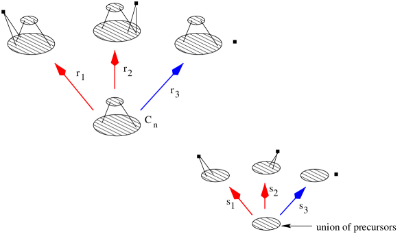
Proof: The top of Figure A.1 shows three children of an arbitrary causal set $C_{n}$. The shaded ellipses represent portions of $C_{n}$. The small square indicates the new element whose birth transforms $C_{n}$ into a causal set $C_{n+1}$ of the next stage. The smaller ellipse “stacked on top of” the larger ellipse represents a subcauset of $C_{n}$ which does not intersect the precursor set of any of the transitions being considered (i.e. none of its elements lie to the past of any of the new elements). This small ellipse thus consists entirely of “spectators” to the transitions under consideration. The bottom part of Figure A.1 shows the corresponding parent and children when these spectators are removed.

Notice that one of the three children is the gregarious child. We will show that the Bell causality equations between this child and each of the others imply all remaining Bell causality equations within this family. Since no Bell causality equation reaches outside a single family (and since, within a family, the Bell causality equations that involve the gregarious child obviously always possess a solution — in fact they determine all ratios of transition probabilities except for that to the timid child), this will prove the lemma.

In the figure $r_{1}$ and $r_{2}$ represent a general pair of transitions related by a Bell causality equation, namely

$$\frac{r_{1}}{r_{2}}=\frac{s_{1}}{s_{2}}\,.$$ (A.1)

But, as illustrated, each of these is also related by a Bell causality equation to the gregarious child, to wit:

$$\frac{r_{1}}{r_{3}}=\frac{s_{1}}{s_{3}}\quad\mbox{and}\quad\frac{r_{2}}{r_{3}}=\frac{s_{2}}{s_{3}}$$ (A.2)

Since (A.1) follows immediately from (A.2), no inconsistencies can arise at stage $n$, and the lemma follows by induction on $n$. $\Box$

Lemma 6

Given Bell causality and the further consequences of general covariance that are embodied in Lemma 2, all the remaining general covariance equations reduce to identities, i.e. they place no further restriction on the parameters of the theory.

Proof:

Figure A.2: Consistency of remaining general covariance conditions

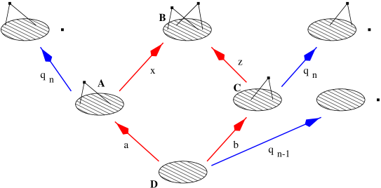
Discrete general covariance states that the probability of forming a causet is independent of the order in which the elements arise, i.e. it is independent of the corresponding path through the poset of finite causets. Now, general covariance relations always can be taken to come from ‘diamonds’ in the poset of causets, for the following reason. As illustrated in Figure A.2, any pair of children of a causet (siblings) will have a common child obtained by adjoining both new elements of the two siblings, i.e. adding to the “grandparent” both the new element which defines one sibling and the new element which defines the other sibling. (For example, consider the case where the 2-antichain     is the grandparent and it has the child    (by adding a disconnected element) and the child     (by adding an element to the future of both elements of     ). To find their common child     add a disconnected element to     , or an element to the future of two of the elements of    .) Now, still referring to Figure A.2, let $|D|=n$ and suppose inductively that all the general covariance relations are satisfied up through stage $n$. A new condition arising at stage $n+1$ says that some path arriving at $B$ via $x$ has the same probability as some other path arriving via $z$. But, by our inductive assumption, each of these paths can be modified to go through $D$ without affecting its probability. Thus, the equality of our two path probabilities reduces simply to $ax=bz$.

Now by Bell causality and lemma 2,

$$\frac{x}{q_{n}}=\frac{b}{q_{n-1}}\,,$$

whence

$$ax=ab\frac{q_{n}}{q_{n-1}}\,.$$

But by symmetry, we also have

$$bz=ba\frac{q_{n}}{q_{n-1}}\,;$$

therefore $ax=bz$, as required. $\Box$

CURRICULUM VITÆ

NAME OF AUTHOR: David Porter Rideout

PLACE OF BIRTH: Huntingdon, PA

DATE OF BIRTH: April 8, 1970

GRADUATE AND UNDERGRADUATE SCHOOLS ATTENDED:
Syracuse University, Syracuse, NY
Georgia Institute of Technology, Atlanta, GA

DEGREES AWARDED:
Master of Science in Physics, 1995, Syracuse University
Bachelor of Aerospace Engineering, 1992, Georgia Institute of Technology

AWARDS AND HONORS:
Sigma Xi Scientific Research Society
Phi Kappa Phi National Honor Society
Tau Beta Pi National Engineering Honor Society
Sigma Gamma Tau National Honor Society in Aerospace Engineering
Golden Key National Honor Society

PROFESSIONAL EXPERIENCE:
Lecturer, Department of Physics, State University of New York, Cortland 2001, 1999
Graduate Research Assistant, Department of Physics, Syracuse University, 1997–2001
Adjunct Professor, Department of Physics, Le Moyne College, 1999, 1998
Teaching Assistant, Department of Physics, Syracuse University, 1992–1998
Engineering Intern, Robinson Industries, Zelienople, PA, 1990–1991

Bibliography

- [1] Noga Alon, Yossi Azar, and Uzi Vishkin. Tight complexity bounds for parallel comparison sorting. In 27th Annual Symposium On Foundations Of Computer Science, pages 502–210. IEEE, IEEE Computer Society Press, 1986.
- [2] Noga Alon, Béla Bollobás, Graham Brightwell, and Svante Janson. Linear extensions of a random partial order. Ann. Applied Prob., 4:108–123, 1994.
- [3] J. Ambjørn, K. N. Anagnostopoulos, and R. Loll. A new perspective on matter coupling in 2d quantum gravity. Phys. Rev. D, 60(104035), 1999.
- [4] J. Ambjørn and R. Loll. Non-perturbative Lorentzian quantum gravity, causality and topology change. Nuclear Physics B, 536:407–434, 1999.
- [5] Jinho Baik, P. Deift, and K. Johansson. On the distribution of the length of the longest increasing subsequence of random permutations. J. Amer. Math. Soc., 12:1119–1178, 1999.
- [6] Jinho Baik and Eric M. Rains. Symmetrized random permutations. 1999. e-print arXive: math.CO/9910019.
- [7] Béla Bollobás and Graham Brightwell. Graphs whose every transitive orientation contains almost every relation. Israel Journal of Mathematics, 59(1):112–128, 1987.
- [8] Béla Bollobás and Graham Brightwell. Transitive orientation of graphs. SIAM J. Comput., 17(6):1119–1133, 1988.
- [9] Béla Bollobás and Graham Brightwell. Box-spaces and random partial orders. Trans. Amer. Math. Soc., 324(1):59–72, March 1991.
- [10] Béla Bollobás and Graham Brightwell. The height of a random partial order: concentration of measure. Ann. Appl. Probab., 2(4):1009–1018, 1992.
- [11] Béla Bollobás and Graham Brightwell. The width of random graph orders. Math. Scientist, 20:69–90, 1995.
- [12] Béla Bollobás and Graham Brightwell. The dimension of random graph orders. In R.L. Graham and J. Nes̆etr̆il, editors, The Mathematics of Paul Erdös II, pages 51–69. Springer-Verlag, 1996.
- [13] Béla Bollobás and Graham Brightwell. The structure of random graph orders. SIAM J. Discrete Math, 10(2):318–335, May 1997.
- [14] Luca Bombelli. Spacetime as a Causal Set. PhD thesis, Syracuse University, December 1987.
- [15] Luca Bombelli. Statistical Lorentzian geometry and the closeness of Lorentzian manifolds. J. Math. Phys, 2000.
- [16] Luca Bombelli, Joohan Lee, David Meyer, and Rafael D. Sorkin. Space-time as a causal set. Physical Review Letters, 59:521–524, 1987.
- [17] Graham Brightwell. Models of random partial orders. In Keith Walker, editor, Surveys in combinatorics, volume 187 of London Math. Soc. Lecture Note Ser., pages 53–83. Cambridge University Press, Cambridge, 1993.
- [18] Graham Brightwell and Ruth Gregory. Structure of random discrete spacetime. Physical Review Letters, 66(3):260–263, January 1991.
- [19] Graham Brightwell, Hans Jürgen Prömel, and Angelika Steger. The average number of linear extensions of a partial order. Journal of Combinatorial Theory, 73:193–206, 1996. Article No. 0017.
- [20] Graham Brightwell and Peter Winkler. Sphereorders. Order, 6(3):235–240, 1989.
- [21] A. Criscuolo and H. Waelbroeck. Causal set dynamics: A toy model. Class. Quantum Grav., 16:1817, 1999. e-print archive: gr-qc/9811088.
- [22] K. Simon D. Crippa and P. Trunz. Markov processes involving -stirling numbers. Combinatorics, Probability and Computing, 6:165–178, 1997.
- [23] Alan Daughton. The Recovery of Locality for Causal Sets and Related Topics. PhD thesis, Syracuse University, 1993.
- [24] Alan Daughton, Rafael D. Sorkin, and C.R. Stephens. Percolation and causal sets: A toy model of quantum gravity. (in preparation).
- [25] Deepak Dhar. Entropy and phase transitions in partially ordered sets. J. Math. Phys., 19(8):1711–1713, August 1978.
- [26] Djamel Dou. Causal Sets, a Possible Interpretation for the Black Hole Entropy, and Related Topics. PhD thesis, SISSA, Trieste, 1999.
- [27] William Feller. An Introduction to Probability Theory and Its Applications, volume I. Wiley, 1957. (In his notation .).
- [28] David Finkelstein. The space-time code. Phys. Rev., 184:1261–71, 1969.
- [29] J.L. Friedman and A. Higuchi. State vectors in higher-dimensional gravity with quantum numbers of quarks and leptons. Nuclear Physics B, 339:491–515, 1990.
- [30] S. W. Hawking. Phys. Rev. D, 46:603–611, 1992.
- [31] Claude Itzykson and Jean-Michel Drouffe. Statistical Field Theory, volume 2. Cambridge University Press, 1989.
- [32] V. A. Kazakov. The appearance of matter fields from quantum fluctuations of 2d-gravity. Mod. Phys. Lett. A, 4:2125–2139, 1989.
- [33] Davide Crippa Klaus Simon and Fabian Collenberg. On the distribution of the transitive closure in a random acyclic digraph. Lecture Notes in Computer Science, 726:345–356, 1993.
- [34] D.J. Kleitman and B.L. Rothschild. The number of finite topologies. Proc. Amer. Math. Society, 25:276–282, 1970.
- [35] D.J. Kleitman and B.L. Rothschild. A phase transition on partial orders. Physica, 96A:254–259, 1979.
- [36] David B. Malament. The class of continuous timelike curves determines the topology of spacetime. J. Mathematical Phys., 18(7):1399–1404, 1977.
- [37] Fotini Markopoulou. Quantum causal histories. Class. Quantum Grav., 17:2059–2072, 2000.
- [38] Xavier Martín, Denjoe O’Connor, David Rideout, and Rafael D. Sorkin. On the “renormalization” transformations induced by cycles of expansion and contraction in causal set cosmology. Phys. Rev D, 63(084026), 2001. e-print archive: gr-qc/0009063.
- [39] David Meyer. Transitive percolation. unpublished notes.
- [40] David A. Meyer. The Dimension of Causal Sets. PhD thesis, Massachusetts Institute of Technology, 1988.
- [41] Jan Myrheim. Statistical geometry. CERN preprint TH-2538 (1978).
- [42] C. M. Newman and L. S. Schulman. One-dimensional percolation models: The existence of a transition for . Commun. Math. Phys., 104(4):547–571, 1986.
- [43] Y. Jack Ng and H. van Dam. A small but nonzero cosmological constant. Int. J. Mod. Phys. D, 1999. e-print arXive: hep-th/9911102.
- [44] Oliver Penrose. Foundations of Statistical Mechanics, volume 22 of International Series of Monographs in Natural Philosophy. Pergamon Press, 1970.
- [45] B. Pittel and R. Tungol. A phase transition phenomenon in a random directed acyclic graph. Technical report, Ohio State, 1998?
- [46] V. N. Plechko. Anticommuting integrals and fermionic field theories for two-dimensional Ising models. August 1997. e-print archive: hep-th/9607053.
- [47] David Reid. Introduction to causal sets: an alternative view of spacetime structure. Canadian Journal of Physics, 79:1–16, 2001. e-print archive: gr-qc/9909075.
- [48] David P. Rideout and Rafael D. Sorkin. Evidence for scaling in the continuum limit of percolated causal sets. (in preparation).
- [49] David P. Rideout and Rafael D. Sorkin. Classical sequential growth dynamics for causal sets. Physical Review D, 61:024002, Jan. 2000. e-print archive: gr-qc/9904062.
- [50] David P. Rideout and Rafael D. Sorkin. Evidence for a continuum limit in causal set dynamics. Phys. Rev. D, 63:104011, 2001. e-print archive: gr-qc/0003117.
- [51] Roberto B. Salgado. Some identities for the quantum measure and its generalizations. 1999. e-print archive: gr-qc/9903015.
- [52] Roberto B. Salgado. PhD thesis, Syracuse University, 2001. (in preparation).
- [53] K. Simon. Improved algorithm for transitive closure on acyclic digraphs. Theoretical Computer Science, 58, 1988.
- [54] Rafael D. Sorkin. First steps with causal sets. In Proceedings of the Conference in honor of Peter G. Bergmann, 1990. Capri, Italy.
- [55] Rafael D. Sorkin. Spacetime and causal sets. In J. C. D’Olivo, E. Nahmad-Achar, M. Rosenbaum, M.P. Ryan, L.F. Urrutia, and F. Zertuche, editors, Relativity and Gravitation: Classical and Quantum, pages 150–173, Singapore, December 1991. World Scientific. (Proceedings of the SILARG VII Conference, held Cocoyoc, Mexico, December, 1990).
- [56] Rafael D. Sorkin. Quantum mechanics as quantum measure theory. Modern Physics Letters A, 9(33):3119–3127, 1994. e-print archive: gr-qc/9401003.
-
[57]
Rafael D. Sorkin.
Forks in the road, on the way to quantum gravity.
Int. J. Th. Phys., 36:2759–2781, 1997.
talk given at the conference entitled “Directions in General Relativity”, held at College Park, Maryland, May, 1993. e-print archive: gr-qc/9706002. - [58] Rafael D. Sorkin. Quantum measure theory and its interpretation. In D.H. Feng and B-L Hu, editors, Quantum Classical Correspondence: Proceedings of the 4th Drexel Symposium on Quantum Nonintegrability, pages 229–251, Cambridge, MA, 1997. International Press. e-print archive: gr-qc/9507057.
[59]
Indications of causal set cosmology.
Int. J. Theor. Phys., 39(7):1731–1736, 2000.
part of the proceedings of the Peyresq IV workshop on Quantum and
Stochastic Gravity, String Cosmology and Inflation held June 28–July 3,
1999 in Peyresq, France.
e-print arXive: gr-qc/0003043. - [60] Richard P. Stanley. Enumerative Combinatorics, volume I. Wadsworth & Brooks/Cole, Monterey, CA, 1986.
- [61] Matthias Staudacher. The yang-lee edge singularity on a dynamical planar random surface. Nuc. Phys. B, 336:349–362, 1990.
- [62] G. ’t Hooft. Quantum gravity: a fundamental problem and some radical ideas. In M. Levy and S. Deser, editors, Recent developments in gravitation, Cargèse Summer School Lectures 1978, page 323, New York/London, 1979. Plenum.
- [63] Mituo Taketani. On formation of the newton mechanics. Supplement of the Progress of Theoretical Physics, 50:53–64, 1971.