Discrete quantum gravity: applications to cosmology

Abstract

We consider the application of the consistent lattice quantum gravity approach we introduced recently to the situation of a Friedmann cosmology and also to Bianchi cosmological models. This allows us to work out in detail the computations involved in the determination of the Lagrange multipliers that impose consistency, and the implications of this determination. It also allows us to study the removal of the Big Bang singularity. Different discretizations can be achieved depending on the version of the classical theory chosen as a starting point and their relationships studied. We analyze in some detail how the continuum limit arises in various models. In particular we notice how remnants of the symmetries of the continuum theory are embodied in constants of the motion of the consistent discrete theory. The unconstrained nature of the discrete theory allows the consistent introduction of a relational time in quantum cosmology, free from the usual conceptual problems.

I Introduction

The use of lattice regularizations in quantum gravity has always been problematic due to the fact that the introduction of the lattice breaks diffeomorphism invariance (see Loll [1] for a review). The lattice theory therefore has a very different symmetry group than the continuum theory it approximates. We have recently introduced [2] a procedure to treat in a consistent way the resulting discrete theories, including their symmetries, both at a classical and quantum mechanical level. As is common in discrete theories, the resulting theory fixes Lagrange multipliers that in the continuum theory are free [3]. This is in principle puzzling and it is worthwhile examining in detail in situations where one can easily control all aspects. In this paper we study these issues in the context of cosmological models: the Friedmann and the Bianchi models. These models have several appealing properties: they have enough degrees of freedom as to have a set of non-trivial observables and make the deparameterization and physical description of the evolution possible, which is a feature one would like to analyze in the full theory. The Bianchi II model is classically soluble through a canonical transformation that maps it to a free particle. One can discretize the model before or after the canonical transformation. The discrete theories are not the same and there is the question as of their similarities and differences. Moreover, generically, other canonical transformations (like the one that introduces the Ashtekar variables) in the continuum will also lead to different theories upon discretization. We will see that the discrete theories avoid the singularity and have symmetries that translate themselves in constants of the motion that are remnants of the observables of the continuum theory. We will see that the discrete theory allows naturally to introduce a relational notion of time free of the usual problems of such approach.

We have recently introduced [2] a general technique for treating the theories that arise when one discretizes a continuum field theory. We have shown that the technique works for Yang–Mills and BF theories and implemented it for the gravitational case. Here we summarize the basic features of the approach. Since lattice field theories have a finite number of degrees of freedom, and since in this paper we are looking at cosmologies only, it suffices to summarize for illustration purposes the technique when applied to a constrained mechanical system.

Consider a constrained mechanical system. We assume we replace in the action all time derivatives with discrete first order finite differences. The time integral in the action is replaced by a sum $S=\sum_{n=1}^{N}L(q_{n},q_{n+1})$ with,

$$L(n,n+1)=p_{n}(q_{n+1}-q_{n})-\epsilon H(q_{n},p_{n})-\lambda_{nB}\phi^{B}(q_{n},p_{n})$$ (1)

where we assume we have a Hamiltonian $H$ and $M$ constraints $B=1\ldots M$ and $\epsilon$ is the time interval. Our formulation works for a system with an arbitrary (finite) number of phase-space degrees of freedom. To simplify the notation we are omitting the indices labeling the degrees of freedom and writing formulae as if the system only had one configuration degree of freedom.

The centerpiece of our technique is to realize that in a theories where time (and space in the case of field theories) is discretized, it makes no sense to work with a Hamiltonian since the latter is the generator of infinitesimal time evolution and one cannot have infinitesimal evolution if time is discrete. The time evolution should be described via a canonical transformation that implements the discrete time evolution between instants $n$ and $n+1$. A type 1 canonical transformation that accomplishes this task has as generating function minus the Lagrangian, viewed as a function of $q_{n}$ and $q_{n+1}$. From it, one obtains the momenta at instant $n+1$

$$P^{q}_{n+1} = {\partial L(n,n+1)\over\partial q_{n+1}}=p_{n}$$ (2)

$$P^{p}_{n+1} = {\partial L(n,n+1)\over\partial p_{n+1}}=0$$ (3)

$$P^{\lambda_{B}}_{n+1} = {\partial L(n,n+1)\over\partial\lambda_{(n+1)B}}=0,$$ (4)

and similarly, the momenta at instant $n$ are given by,

$$P^{q}_{n} = -{\partial L(n,n+1)\over\partial q_{n}}=p_{n}+\epsilon{\partial H(q_{n},p_{n})\over\partial q_{n}}+\lambda_{nB}{\partial\phi^{B}(q_{n},p_{n})\over\partial q_{n}}$$ (5)

$$P^{p}_{n} = -{\partial L(n,n+1)\over\partial p_{n}}=-(q_{n+1}-q_{n})+\epsilon{\partial H(q_{n},p_{n})\over\partial p_{n}}+\lambda_{nB}{\partial\phi^{B}(q_{n},p_{n})\over\partial p_{n}}$$ (6)

$$P^{\lambda_{B}}_{n} = \phi^{B}(q_{n},p_{n}).$$ (7)

We can now combine these equations to give,

$$p_{n}-p_{n-1} = -\epsilon{\partial H(q_{n},p_{n})\over\partial q_{n}}-\lambda_{nB}{\partial\phi^{B}(q_{n},p_{n})\over\partial q_{n}}$$ (8)

$$q_{n+1}-q_{n} = \epsilon{\partial H(q_{n},p_{n})\over\partial p_{n}}+\lambda_{nB}{\partial\phi^{B}(q_{n},p_{n})\over\partial p_{n}}$$ (9)

$$\phi^{B}(q_{n},p_{n}) = 0.$$ (10)

Superficially, these equations appear entirely equivalent to the continuum ones. However, they hide the fact that in order for the constraints to be preserved, the Lagrange multipliers get fixed. Another way to see it, is that $P^{q}_{n+1}=p_{n}$ and therefore it is immediate that the Poisson bracket of the constraints evaluated at $n$ and at $n+1$ is non-vanishing. It is illuminating to rewrite these equations in terms of the canonically conjugate pair,

$$P^{q}_{n+1}-P^{q}_{n} = -\epsilon{\partial H(q_{n},P^{q}_{n+1})\over\partial q_{n}}-\lambda_{nB}{\partial\phi^{B}(q_{n},P^{q}_{n+1})\over\partial q_{n}}$$ (11)

$$q_{n+1}-q_{n} = \epsilon{\partial H(q_{n},P^{q}_{n+1})\over\partial P^{q}_{n+1}}+\lambda_{nB}{\partial\phi^{B}(q_{n},P^{q}_{n+1})\over\partial P^{q}_{n+1}}$$ (12)

$$\phi^{B}(q_{n},P^{q}_{n+1}) = 0.$$ (13)

We therefore will eliminate the “constraints” (13) by solving them for the Lagrange multipliers. One can proceed in various ways, either determining the Lagrange multipliers at time $n$ as functions of the variables at either $n,n-1$ or $n+1$. We will choose to determine the Lagrange multipliers at instant $n$ as functions of $P^{q}_{n}$ and $q_{n}$ in this paper. For different problems it can be more convenient to make one choice over the other. In all cases solving for the Lagrange multipliers implies solving algebraic equations, but depending on the choices made the resulting equations can be quite non-linear and guaranteeing that they will have real solutions can be problematic. For the examples of this paper we have found that the choice we make is the most convenient one.

We solve (11) for $P^{q}_{n+1}$ and substitute it in the “constraint” (13) and obtain

$$\phi^{B}(q_{n},P^{q}_{n},\lambda_{nB})=0,$$ (14)

and this constitutes a system of equations. Generically, these will determine

$$\lambda_{nB}=\lambda_{nB}(q_{n},P^{q}_{n},v^{\alpha})$$ (15)

where the $v^{\alpha}$ are a set of free parameters that may arise if the system of equations is undetermined. The eventual presence of these parameters will signify that the resulting theory still has a genuine gauge freedom represented by freely specifiable Lagrange multipliers.

The final set of evolution equations for the system is therefore given by (11,12) where the Lagrange multipliers are substituted using (15).

This construction raises several questions about how to implement it in concrete gravitational examples. We would like to probe these questions in the context of cosmological models. The main points we want to probe are the following:

(i) Solubility of the multiplier equations: Solving the constraints by choosing the Lagrange multipliers produces a theory that is constraint free. This is analogous to what happens when one gauge fixes a theory. It is well known that gauge fixing is not a cure for the problems of general relativity since gauge fixings usually become problematic. In the same sense, it could happen that the algebraic equations that determine the Lagrange multipliers (the lapse and the shift in the case of general relativity) in our approach develop problems in their solutions (for instance, negative lapses, or complex solutions). We will show that in these simple examples there do not appear to be difficulties even in situations where a traditional gauge fixing in the continuum theory is not possible.

(ii) Performing meaningful comparisons: When comparing a discrete theory with a continuum theory, one needs to choose the quantities that are to be compared. In particular, the continuum theory has “observables” (“perennials”), that is, quantities that have vanishing Poisson brackets with the constraints. The discrete theory is constraint-free. We will see that one has exact conserved quantities in the discrete theory that are consequences of remnant symmetries encoded in the initial data that the discrete theory inherits from the continuum theory. The conserved quantities will turn out to be closely related to the observables of the continuum theory.

(iii) The continuum limit: in continuum constrained theories with first class constraints, the Lagrange multipliers are free functions. Yet in our discrete construction, the Lagrange multipliers are determined by the initial conditions. If one wishes to take a naive continuum limit, the discrete equations that determine the Lagrange multipliers must become ill-defined. To extract meaningful information about the continuum theories, one needs to proceed differently. We have already mentioned that the discrete theories are constraint-free, since one solves the constraints for the Lagrange multipliers. This in particular means that they have more degrees of freedom than the continuum theory they are trying to approximate. The continuum limit might be achieved by a careful fine tuning of the extra degrees of freedom, or might occur in certain asymptotic regions of the dynamics as an attractor for a large set of initial values of the extra degrees of freedom. We will exhibit examples of both kinds of behaviors.

(iv) Singularities: Discrete theories in principle have the possibility of evolving through a Big Bang singularity, since generically the singularity will not lie on a point on the lattice. However, we will see that if one uses canonical variables such that the singularity is at a boundary of the range of a variable, then the discrete theories do develop singularities, although they can be avoided in certain cases.

(v) Problem of time: We will discuss how to obtain evolution in the discrete by using a relational approach in terms of the observables of these theories. This suggests that the problem of time can be solved in these theories.

(vi) Discretization ambiguities: An important element is to note that the Lagrange multipliers get determined by this construction only if the constraint is both a function of $q$ and $p$. If the constraint is only a function of $q$ or of $p$ then the constraints are automatically preserved in evolution without fixing the Lagrange multipliers. This raises a conceptual question. For certain theories in the continuum, one can make a canonical transformation to a new set of variables such that the constraints depend only on $q$ or on $p$. The resulting discrete theories will therefore be very different in nature, but will have the same continuum limit. From the point of view of using discrete theories to quantize gravity, we believe this ambiguity should receive the same treatment that quantization ambiguities (choice of canonical variables, factor orderings, etc.) get: they are decided experimentally. Generically there will be different discrete theories upon which to base the quantization and some will be better at approximating nature than others in given regimes. Many of them may allow to recover the continuum limit, however they may have different discrete properties when one is far from the semiclassical regime.

The organization of this paper is as follows: in the next section we discuss several Friedmann models that exhibit various behaviors upon discretization. In section III we discuss the quantization of the models and the various possibilities concerning how one approaches the “problem of time”. In section IV we discuss other models, including the Bianchi ones and show that they exhibit similar kinds of behaviors as the ones we encountered in the Friedmann models. We end with a discussion of the importance of the results.

II Friedmann models

A Continuum theory

We will consider a Friedmann cosmological model, written in terms of Ashtekar’s variables [4]. The fundamental canonical pair is $(E,A)$ where $E$ is the only remnant of the triad after the minisuperspace reduction and $A$ is its canonically conjugate variable. We will consider the presence of a cosmological constant and of a scalar field. We will assume the scalar field has a very large mass so we can neglect its kinetic term in the Hamiltonian constraint, for the sake of computational simplicity. The Lagrangian for the model is,

$$L=E\dot{A}+\pi\dot{\phi}-NE^{2}(-A^{2}+(\Lambda+m^{2}\phi^{2})|E|)$$ (16)

where $\Lambda$ is the cosmological constant, $m$ is the mass of the scalar field $\phi$, $\pi$ is its canonically conjugate momentum and $N$ is the lapse with density weight minus one. The appearance of $|E|$ in the Lagrangian is due to the fact that the term cubic in $E$ is supposed to represent the spatial volume and therefore should be positive definite. In terms of the ordinary lapse $\alpha$ we have $\alpha=N|E|^{3/2}$. The equations of motion and constraint are

$$\dot{A} = N(\Lambda+m^{2}\phi^{2}){\rm sgn}(E)E^{2}$$ (17)

$$\dot{E} = 2NE^{2}A$$ (18)

$$\dot{\phi} = 0$$ (19)

$$\dot{\pi} = -2N|E|^{3}m^{2}\phi$$ (20)

$$A^{2} = (\Lambda+m^{2}\phi^{2})|E|$$ (21)

It immediately follows from the large mass approximation that $\phi={\rm constant}$. To solve for the rest of the variables, we need to distinguish four cases, depending on the signs of $E$ and $A$. Let us call $\epsilon={\rm sgn}(E)$ and $\chi={\rm sgn}(A)$. Then the solution (with the choice of lapse $\alpha=1$) is,

$$A = \chi\exp\left(\chi\epsilon t\sqrt{\Lambda+m^{2}\phi^{2}}\right)$$ (22)

$$E = \epsilon{\exp\left(2\chi\epsilon t\sqrt{\Lambda+m^{2}\phi^{2}}\right)\over{\Lambda+m^{2}\phi^{2}}}$$ (23)

There are four possibilities according to the signs $\epsilon,\chi$. If $\epsilon=\chi=1$ or $\epsilon=\chi=-1$ we have a universe that expands. If both have different signs, the universe contracts. This just reflects that the Lagrangian is invariant if one changes the sign of either $A$ or $E$ and the sign of time. It is also invariant if one changes simultaneously the sign of both $A$ and $E$.

Let us turn to the observables of the theory (quantities that have vanishing Poisson brackets with the constraint (21) and therefore are constants of the motion). The theory has four phase space degrees of freedom with one constraint, therefore there should be two independent observables. Immediately one can construct an observable $O_{1}=\phi$, since the latter is conserved due to the large mass approximation. To construct the second observable we write the equation for the trajectory,

$${d\pi\over dA}={-2Em^{2}\phi\over\Lambda+m^{2}\phi^{2}}=-{2A^{2}m^{2}\phi\over\left(\Lambda+m^{2}\phi^{2}\right)^{2}}{\rm sgn}E$$ (24)

where in the latter identity we have used the constraint. Integrating, we get the observable,

$$O_{2}=\pi+{2\over 3}{m^{2}\phi\over\left(\Lambda+m^{2}\phi^{2}\right)^{2}}A^{3}{\rm sgn}E$$ (25)

and using the constraint again we can rewrite it,

$$O_{2}=\pi+{2\over 3}{m^{2}\phi\over\Lambda+m^{2}\phi^{2}}AE.$$ (26)

Although the last two expressions are equivalent, we will see that upon discretization only one of them becomes an exact observable of the discrete theory.

B Discrete theory

We consider the evolution parameter to be a discrete variable. Then the Lagrangian becomes

$$L(n,n+1)=E_{n}(A_{n+1}-A_{n})+\pi_{n}(\phi_{n+1}-\phi_{n})-N_{n}E_{n}^{2}(-A^{2}_{n}+(\Lambda+m^{2}\phi^{2}_{n})|E_{n}|)$$ (27)

The discrete time evolution is generated by a canonical transformation of type 1 whose generating function is given by $-L$, viewed as a function of the configuration variables at instants $n$ and $n+1$. The canonical transformation defines the canonically conjugate momenta to all variables. The transformation is such that the symplectic structure so defined is preserved under evolution. The configuration variables will be $(A_{n},E_{n},\pi_{n},\phi_{n},N_{n})$ with canonical momenta $(P^{A}_{n},P^{E}_{n},P^{\phi}_{n},P^{\pi}_{n},P^{N}_{n})$, defined by,

$$P^{E}_{n+1} = {\partial L(n,n+1)\over\partial E_{n+1}}=0,$$ (28)

$$P^{E}_{n} = -{\partial L(n,n+1)\over\partial E_{n}}=-(A_{n+1}-A_{n})+N_{n}E^{2}_{n}(\Lambda+m^{2}\phi^{2}_{n}){\rm sgn}E_{n},$$ (29)

$$P^{A}_{n+1} = {\partial L(n,n+1)\over\partial A_{n+1}}=E_{n},$$ (30)

$$P^{A}_{n} = -{\partial L(n,n+1)\over\partial A_{n}}=E_{n}-2N_{n}A_{n}E_{n}^{2},$$ (31)

$$P^{\phi}_{n+1} = {\partial L(n,n+1)\over\partial\phi_{n+1}}=\pi_{n},$$ (32)

$$P^{\phi}_{n} = -{\partial L(n,n+1)\over\partial\phi_{n}}=\pi_{n}+2N_{n}E_{n}^{2}m^{2}\phi_{n}|E_{n}|,$$ (33)

$$P^{\pi}_{n+1} = {\partial L(n,n+1)\over\partial\pi_{n+1}}=0,$$ (34)

$$P^{\pi}_{n} = -{\partial L(n,n+1)\over\partial\pi_{n}}=-\phi_{n+1}+\phi_{n},$$ (35)

$$P^{N}_{n+1} = {\partial L(n,n+1)\over\partial N_{n+1}}=0,$$ (36)

$$P^{N}_{n} = -{\partial L(n,n+1)\over\partial N_{n}}=E_{n}^{2}(-A^{2}_{n}+(\Lambda+m^{2}\phi^{2}_{n})|E_{n}|).$$ (37)

These equations can be recast into a more familiar looking fashion, by combining the information at levels $n$ and $n+1$,

$$A_{n+1}-A_{n} = N_{n}(P^{A}_{n+1})^{2}_{n}(\Lambda+m^{2}\phi^{2}_{n}){\rm sgn}P^{A}_{n+1},$$ (38)

$$P^{A}_{n+1}-P^{A}_{n} = 2N_{n}A_{n}(P^{A}_{n+1})^{2}$$ (39)

$$\phi_{n+1}-\phi_{n} = 0$$ (40)

$$P^{\phi}_{n+1}-P^{\phi}_{n} = -2N_{n}(P^{A}_{n+1})^{2}m^{2}\phi_{n}|P^{A}_{n+1}|,$$ (41)

$$0 = -A^{2}_{n}+(\Lambda+m^{2}\phi^{2}_{n})|P^{A}_{n+1}|,$$ (42)

and the phase space is now spanned by $A_{n},P^{A}_{n},\phi_{n},P^{\phi}_{n}$.

Enforcing the constraint (42) leads to the determination of the Lagrange multipliers. There are two ways to proceed. We can use the evolution equation (39) to eliminate $P^{A}_{n+1}$ in the constraint. The latter will therefore be an equation that determines $N_{n}$ as a function of $P^{A}_{n},A_{n},\phi_{n}$. The alternative is to use (38,40) to eliminate $A_{n}$ and $\phi_{n}$. This would yield $N_{n}$ as a function of $P^{A}_{n+1},\phi_{n+1},A_{n+1}$. We will here follow the first approach since it is the more natural one to track evolution forward in the parameter $n$.

From (39) we determine,

$$P^{A}_{n+1}={1+\xi\sqrt{1-8P^{A}_{n}A_{n}N_{n}}\over 4A_{n}N_{n}},$$ (43)

where $\xi=\pm 1$ and we will see the final solution is independent of $\xi$. Substituting in (42) and solving for the lapse we get,

$$N_{n}={\left[-P^{A}_{n}\left(\Lambda+m^{2}\phi_{n}^{2}\right)+A_{n}^{2}{\rm sgn}P^{A}_{n}\right]\left(\Lambda+m^{2}\phi_{n}^{2}\right)\over 2A_{n}^{5}}.$$ (44)

Let us summarize how the evolution scheme presented actually operates. Let us assume that some initial data $A^{(0)},P^{A}_{(0)}$, satisfying the constraints of the continuum theory, are to be evolved. The recipe will consist of assigning $A_{0}=A^{(0)}$ and $P^{A}_{1}=P^{A}_{(0)}$. Notice that this will automatically satisfy (42). In order to the scheme to be complete we need to specify $P^{A}_{0}$. This is a free parameter. Once it is specified, then the evolution equations will determine all the variables of the problem, including the lapse. Notice that if one chooses $P^{A}_{0}$ such that, together with the value of $A_{0}$ they satisfy the constraint, then the right hand side of the equation for the lapse (44) would vanish and no evolution takes place. It is clear that one can choose $P^{A}_{0}$ in such a way as to make the evolution step as small as desired.

The equation for the lapse (44) implies that the lapse is a real number for any real initial data. But it does not immediately imply that the lapse is positive. However, it can be shown that the sign of the lapse, once it is determined by the initial configuration, does not change under evolution. The proof is tedious since one has to separately consider the various possible signs of $\epsilon$ and $\chi$. Let us exhibit the proof for the case $\epsilon=\chi=1$. Then $A_{n}>0$ and $P_{n}>0$. To simplify the notation let us set $\Theta=\Lambda+m^{2}\phi^{2}$, which is a positive quantity. The equation determining the lapse becomes,

$$N_{n}={\left[-P_{n}^{A}\Theta+A^{2}_{n}\right]\Theta\over 2A_{n}^{5}}.$$ (45)

Let us assume we start with a positive lapse, i.e., $A_{n}^{2}/\Theta>P_{n}$. The equations of motion then imply $A_{n+1}>A_{n}$ and $P^{A}_{n+1}>P^{A}_{n}$. If we now compute the lapse in the next instant of time we get,

$$N_{n+1}={\left[-P_{n+1}^{A}\Theta+A_{n+1}^{2}\right]\Theta\over 2A_{n+1}^{5}}={\left[-A_{n}^{2}+A_{n+1}^{2}\right]\over 2A_{n+1}^{5}}>0$$ (46)

where in the last step we used the constraint. Notice that if one had chosen initial values such that $N_{n}<0$, then $A_{n+1}<A_{n}$ and $P_{n+1}<P_{n}$ and the equation for is $N_{n+1}<0$. In effect, one is following the same trajectory backwards in time, i.e. the universe contracts instead of expanding. A similar analysis holds for the other choices of $\epsilon$ and $\chi$.

This is an important result. In spite of the simplicity of the model, there was no a priori reason to expect that the construction would yield a real lapse. Or that upon evolution the equation determining the lapse could not become singular or imply a change in the sign of the lapse, therefore not allowing a complete coverage of the classical orbits in the discrete theory.

We would like to address the issue of how to compare the discrete theory with the continuum one. Notice that this is a priori a delicate proposition. The continuum theory has a constraint and therefore a gauge symmetry. The discrete theory is constraint-free. A direct comparison of a given variable in the continuum theory with its discrete counterpart is therefore not adequate, since one could be comparing a solution with its counterpart in not necessarily the same gauge. This suggests that a more meaningful comparison could be attempted if one considered the observables of the continuum theory, since the latter are gauge independent. Even this is a priori problematic. In the discrete theory, since there are no constraints, any quantity is an observable. One could consider quantities in the discrete theories that arise as discretizations of the observables of the continuum theory. But due to discretization ambiguities, there are many discrete counterparts to each observable in the continuum. All of them are “observables” of the discrete theory since there are no constraints. Is there any that is preferred? We will show that indeed one can find discretizations of the observables of the continuum theory that are exact constants of the motion of the discrete theory.

In order to exhibit this, we start by rewriting evolution equations that result from determining the lapse as discussed above. We make them explicit for $\epsilon=1$,

$$P^{A}_{n+1} = A_{n}^{2}\Theta^{-1}$$ (47)

$$A_{n+1} = {3A_{n}^{2}-P^{A}_{n}\Theta\over 2A_{n}}$$ (48)

$$\phi_{n+1} = \phi_{n}$$ (49)

$$P^{\phi}_{n+1} = P^{\phi}_{n}-\left(A_{n}^{3}-P^{A}_{n}\Theta A_{n}\right)m^{2}\phi_{n}\Theta^{-2}$$ (50)

where we recall that $\Theta=\Lambda+m^{2}\phi_{n}^{2}$. It should be noted that these equations preserve the symplectic structure, that is, the variables $(P^{q}_{n+1},q_{n+1})$ have the same canonical Poisson brackets as $(P^{q}_{n},q_{n})$. The resulting dynamical system has four phase space degrees of freedom. This is in contrast to the system in the continuum, that had four phase space degrees of freedom with one first class constraint, resulting in only two phase space degrees of freedom. This appears as surprising, since one seems to be attempting to approximate a theory with two degrees of freedom with a discrete theory that has four degrees of freedom. To understand this better, let us consider the issue of the observables of the continuum theory and their discrete counterpart. We will see that the discrete theory appears to have hidden symmetries that may help explain why it approximates correctly a theory with in principle a different number of degrees of freedom.

Let us recall the continuum expression of the non-trivial observable we found,

$$O=\pi+{2\over 3}{m^{2}\phi\over\Lambda+m^{2}\phi^{2}}AE.$$ (51)

If we consider one possible discretization of this expression,

$$O_{n}=P^{\phi}_{n}+{2\over 3}{m^{2}\phi_{n}\over\Theta_{n}}A_{n}P^{A}_{n},$$ (52)

we can check that the discrete equations of motion immediately imply $O_{n+1}=O_{n}$. That is, this expression is an exact constant of the motion of the discrete theory. This is a rather remarkable result. It is not at all true that a generic discretization of an observable of the continuum theory will yield a constant of the motion of the discrete theory. For instance, if we had started from (25) and discretized it, one would not get a constant of the motion. A further ambiguity arises in the fact that we have made the choice for all elements of the right hand-side to be at the level $n$ when discretizing.

It is also remarkable that the discrete theory would have constants of the motion, and more remarkable that such constants of the motion can be obtained by discretization of the observables of the continuum theory. We do not know if this is a generic feature of discretized theories or if it just is something that occurs in some examples.

In general the discrete theory, having more degrees of freedom than the continuum theory, will have more constants of the motion than observables in the continuum theory. In this example, the discrete theory has four degrees of freedom. One can find four constants of the motion. One of them we already discussed. The other one is $\phi$. The two other constants of the motion can in principle be worked out. One of them is a measure of how well the discrete theory approximates the continuum theory and is only a function of the canonical variables (it does not depend explicitly on $n$). The constant of the motion is associated with the canonical transformation that performs the evolution in $n$. It is analogous to the Hamiltonian of the discrete theory. The expression can be worked out as a power series involving the discrete expression of the constraint of the continuum theory. This constant of motion therefore vanishes in the continuum limit. The other constant of the motion also vanishes in the continuum limit.

That is, we have two of the constants of the motion that reduce to the observables of the continuum theory in the continuum limit and two others that vanish in such limit. The discrete theory therefore clearly has a remnant of the symmetries of the continuum theory. The canonical transformations associated with the constants of the motion which have non-vanishing continuum limit map dynamical trajectories to other trajectories that can be viewed as different choices of lapse in the discrete theory. This is the discrete analog of the reparameterization invariance of the continuum theory. As we will see in the next section the lapse in the discrete theory is determined up to two constants. The choice of these two constants is the remnant of the reparameterization invariance of the continuum theory that is present in the discrete theory.

C Comparing the discrete and the continuum theories

We would like to compare the predictions of the discrete theory with those of the continuum theory. Since we are comparing two theories that are different in nature, one has to provide a mapping between them. We start by identifying the variables $t=\epsilon n$ in the continuum and discrete theories respectively where $\epsilon$ is a real positive quantity. The discrete theory provides a unique solution given initial data, including a lapse function. We therefore should cast the continuum theory with a lapse that is close to the one generated by the discrete theory, otherwise the comparison would not be meaningful. In order to do this, we first derive a recurrence relation for the variable $A_{n}$. We obtain it by combining eqs. (47,48),

$$A_{n+1}={3A_{n}^{2}-A_{n-1}^{2}\over 2A_{n}}.$$ (53)

We now write an equation in the continuum such that its discretization would yield this recursion relation,

$$2A\ddot{A}+\dot{A}^{2}=0,$$ (54)

where we approximate $\ddot{A}=(A_{n+1}+A_{n-1}-2A_{n})/\epsilon^{2}$ and $\dot{A}=(A_{n+1}-A_{n})/\epsilon$. The solution of the differential equation is, $A=C_{A}(t+k)^{2/3}$ for $t+k>0$ where $C_{A}$ and $k$ are constants that will depend on the initial values specified to the recursion relation $A_{0}$ and $A_{1}$. This corresponds to one of the four branches we considered before. If we now consider the constraint, this would determine $E$ as a function of the parameter $t$. Substituting $E$ and $A$ in the continuum evolution equations one obtains an algebraic equation for the densitized lapse $N$. The solution is $N=C_{N}/(t+k)^{3}$, the ordinary lapse is $\alpha=C_{\alpha}/(t+k)$ where $C_{N}$ and $C_{\alpha}$ are again constants that are determined by the initial values of the recursion relation. We therefore see that the discrete theory has a remnant of the reparameterization symmetry of the continuum theory: in the continuum limit it can reproduce a two parameter family of functional forms of the lapse.

Figure (1) shows the discrete evolution of $E$ and $A$. The branch chosen is such that one has a universe that first contracts and then expands. We have chosen the parameter in such a way that the point where one would expect the singularity occurs at $n=0$.

,

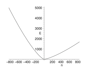
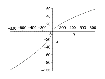
FIG. 1.: The discrete evolution of the triad $E$ and the connection $A$ as a function of the discrete evolution parameter $n$. We have chosen initial conditions that produce a positive branch of $A$ for $n>0$ and a negative branch for $n<0$. For the triad we chose both branches positive.

Although the graphs suggest that the triad goes to zero at $n=0$ and therefore one has a singularity, this is not the case. Figure (2) shows in more detail the approach to $n=0$. It also includes superposed on it the continuum solution. As we see, the continuum solution indeed goes to zero at $t=0$. The discrete solution takes a small but non-zero value. One could choose initial data such that the discrete solution becomes singular, but it would correspond to a set of measure zero of initial data. Generically, the singularity is avoided in the discrete theory.

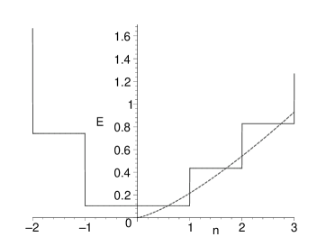
FIG. 2.: The approach to the singularity in the discrete and continuum solutions. The discrete theory has a small but non-vanishing triad at $n=0$ and the singularity is therefore avoided.

One can also notice that while going through the singularity the universe re-expands, but the behavior at both sides of the singularity is different. In this sense the discrete cosmology may implement the proposal of Smolin [5] that different physics takes place when one goes through a singularity.

In figure (3) we show the level of agreement between the discrete and continuum solutions for the triad. If we take a larger scale the two curves are indistinguishable.

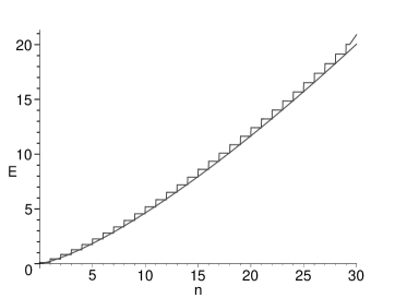
FIG. 3.: Agreement between the continuum and discrete solutions for the triad.

A better idea of the agreement between the continuum and the discrete theory can be obtained by evaluating the Hamiltonian constraint of the continuum theory in the discrete theory. The constraint reads $A^{2}-E\Theta=0$, if we discretize it as $A^{2}_{n}-P^{A}_{n}\Theta_{n}$ this in general is not zero in the discrete theory, what vanishes is equation (42), which is different. Figure (4) shows a measure of how well the constraint of the continuum theory is satisfied. In order to normalize the result in a meaningful way (since the quantity is supposed to be zero) we plot $H_{norm}=1-A^{2}_{n}/P^{A}_{n}\Theta$.

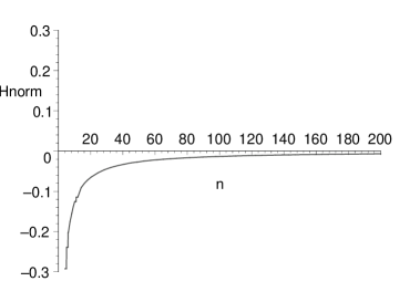
FIG. 4.: A normalized measure of the Hamiltonian constraint of the continuum theory (see text for details), evaluated in the discrete theory. We see that the constraint is better satisfied at later times, indicating that the discrete theory is achieving a continuum limit.

The presence of the two constants of motion in the discrete theory implies two relations between the dynamical variables of the theory. If one combines these relations with the constraint of the continuum theory, one will obtain further relations among the dynamical variables that will hold only approximately, since the constraint of the continuum theory is not exactly satisfied in the discrete theory. However, due to the results shown in figure 4, these relations will approximate well the relations that appear in the continuum theory as a consequence of the observables present in such theories, and their combination with the constraint of the continuum theory. It is to be noted that the latter are relationships among the variables of the continuum theory that are parameterization independent. The agreement between the continuum and discrete theory at the level of these relations indicates that both are agreeing at a gauge invariant level.

As an example of this, in figure 5 we display the difference between the value of the variable $P^{\phi}_{n}$ computed directly from the evolution of the discrete theory and its value computed using the continuum relation (25) translated to the discrete theory,

$$P^{\phi}_{n}=O_{2}-{2\over 3}{m^{2}\phi_{n}\over\left(\Lambda+m^{2}\phi_{n}^{2}\right)^{2}}A_{n}^{3}.$$ (55)

Since $P^{\phi}_{n}$ grows as $n^{2}$ in this example, we show in the figure the difference between the $P^{\phi}_{n}$ calculated both ways divided by the norm of the exact value of $P^{\phi}_{n}$.

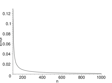
FIG. 5.: The difference between the value of the variable $P^{\phi}_{n}$ calculated directly from the evolution equations and by inferring it from the equation that defines the observable in the continuum theory. As one enters the region where the discrete theory describes the continuum well this difference goes to zero. We plot the difference divided by the value of $P^{\phi}$ since the latter grows and therefore the difference also increases in value, but decreases in relative value.

III Quantization

One of the main attractive features of the consistent discrete lattice approach is that the resulting discrete theory is free of constraints. This implies that many of the deep conceptual problems of quantum gravity appear to be eliminated from the outset. As we will see, this is not necessarily the case. We will see that the quantization of the model is more subtle that what one would initially attempt and that there are several possibilities for quantization, depending on the attitude one adopts with respect to the “problem of time”.

A Naive quantization

Given that the theory is unconstrained, and that time evolution is represented by a canonical transformation, it appears that one can readily quantize the system. One starts by picking a polarization, for instance wavefunctions $\Psi[A,\phi]$. It is natural to operate in the Heisenberg picture. In this picture operators are labeled by the “time level” $n$. Operators $\hat{A}_{0}$ and $\hat{\phi}_{0}$ act multiplicatively and $\hat{P^{A}}_{0}=i{\partial/\partial A}$ and $\hat{P^{\phi}}_{0}=i{\partial/\partial\phi}$. Wavefunctions are square integrable functions $A$ and $\phi$ and the fundamental operators are self-adjoint on this space. Operators at other instances of “time” are obtained via a unitary transformation. This is guaranteed by the fact that in the classical theory the discrete time evolution was implemented via a canonical transformation. The usual problem of the dynamics of a canonical quantization, i.e. implementing the Hamiltonian as an operator in a certain factor ordering translates here into finding a unitary operator that implements at an operatorial level the classical discrete equations of motion for the system.

To construct the unitary operator we start by writing the following matrix elements,

$$<p,\phi_{1},n|U|A,\phi_{2},n>=<p,\phi_{1},n+1|A,\phi_{2},n>,$$ (56)

where $<p,\phi,n|$ and $|A,\phi,n>$ are bases of states at instant $n$ labeled by the Eigenvalues of $\hat{\phi}_{n}$ and $\hat{P^{A}}_{n}$ and $|A,\phi,n>$ respectively, which we denote by $p$ and $A$.

We now consider the matrix elements of the operatorial version of equation (47),

$$<p,\phi_{1},n+1|\hat{|P^{A}_{n+1}|}-\hat{A}_{n}^{2}\hat{\Theta}_{n}^{-1}|A,\phi_{2},n>=\left(|P^{A}|-A^{2}\Theta^{-1}\right)<p,\phi_{1},n+1|A,\phi_{2},n>=0.$$ (57)

This implies that

$$<p,\phi_{1},n+1|A,\phi_{2},n>=f(A,\phi_{1},\phi_{2})\delta\left(|p|-A^{2}\Theta^{-1}\right)$$ (58)

with $f(A,\phi_{1},\phi_{2})$ an arbitrary normalization factor. This factor can be determined by studying in a similar fashion the other evolution equations. The final result for the unitary evolution operator is,

$$<p,\phi_{1},n+1||A,\phi_{2},n> = \sqrt{2|A|\over\Theta}\delta\left(p-{A^{2}\over\Theta}\right)\delta(\phi_{1}-\phi_{2})\exp\left(i{A^{3}\over\Theta}\right)H(A)$$ (59)

$$+ \sqrt{2|A|\over\Theta}\delta\left(p+{A^{2}\over\Theta}\right)\delta(\phi_{1}-\phi_{2})\exp\left(-i{A^{3}\over\Theta}\right)H(-A)$$ (60)

where $H(A)$ is the Heaviside function $H(A)=1\forall A>0$, zero otherwise.

One can Fourier transform to obtain the matrix elements in the $|A,\phi,n>$ basis,

$$<A_{1},\phi_{1},n+1|A_{2},\phi_{2},n> = \sqrt{2|A_{2}|\over\Theta}\exp\left(-i{A^{2}_{2}(A_{1}-A_{2})\over\Theta}\right)\delta(\phi_{1}-\phi_{2})H(A_{2})$$ (61)

$$+ \sqrt{2|A_{2}|\over\Theta}\exp\left(i{A^{2}_{2}(A_{1}-A_{2})\over\Theta}\right)\delta(\phi_{1}-\phi_{2})H(-A_{2}).$$ (62)

Dirac [6] had already noted in 1933 that the unitary operator that implements a canonical transformation is given by $\exp(-iG)$ where $G$ is the generating function of the canonical transformation. In our case the generating function (after eliminating the Lagrange multipliers is indeed given by $G(A_{n},A_{n+1})=A^{2}_{n}(A_{n+1}-A_{n})/\Theta$. There is an overall difference with Dirac’s result since he chooses a specific factor ordering that does not coincide with the one we chose. It is interesting that this construction is what led Dirac to the notion of path integral.

With this unitary transformation one can answer any question about evolution in the Heisenberg picture for the model in question. One could also choose to work in the Schrödinger picture, evolving the states. Notice that the wavefunctions admit a genuine probabilistic interpretation. This is in distinct contrast with the usual “naive Schrödinger interpretation” of quantum cosmology which attempted to ascribe probabilistic value to the square of a solution of the Wheeler–DeWitt equation (see [7] for a detailed discussion of the problems associated with the naive interpretation).

An interesting aspect of this quantization is that for any square-integrable wavefunction and for any value of the parameter $n$, the expectation value of $(P^{A}_{n})^{2}$, and therefore that of $E^{2}$ is non-vanishing, and so are the metric and the volume of the slice. Therefore quantum mechanically one never sees a singularity. This was expected, classically the singularity only occurred for a set of measure zero of initial conditions in the discrete theory and therefore quantum mechanically, since we are superposing many initial conditions, the singularity has zero probability. We therefore have a similar prediction to the one Bojowald [8] encountered in his approach to quantum cosmology in the loop representation, but the details of how the singularity is avoided are quite different. For instance, in Bojowald’s approach there is an instant in the evolution in which the volume goes through zero and nevertheless the inverse scale factor is finite. The metric is not a well defined operator at all. Here the volume never goes through zero, the inverse scale factor and the metric are always finite.

Although the attempted quantization is complete, its interpretation as a quantum theory of cosmology, is problematic. This has to do with the fact that the “evolution” variable $n$ does not have any intrinsic meaning. Classically there is no combination of the variables of the problem that would tell us what the value of $n$ is. There is no well defined notion of “future” and “past” since a generic quantum state will be a superposition of expanding and contracting universes (recall that in this approach the initial data determine if the universe expands or contracts). Therefore the quantum theory, although complete, is lacking in predictive power.

B “Gauge fixed” quantization

The formulation of the theory we considered for quantization in the last section is such that the same orbit of the continuum theory is represented by many orbits in the discrete theories, dependent on the initial data specified, as we discussed in section II C. One could therefore attempt a quantization after eliminating such remnant symmetry. This would be tantamount to a “gauge fixed” quantization. In order to do this we choose two constants $T^{0},T^{1}$ and set $T^{0}=A_{0}$ and $T^{1}=A_{1}$, which also determines $P^{A}_{0}=3(T^{0})^{2}-2T^{0}T^{1}/\Theta$. We can from this eliminate completely the variables $A_{n}$ and $P^{A}_{n}$ from the theory and use the variable $T^{n}=A^{n}$ as a time variable.

The theory now has as variables $\phi_{n},P^{\phi}_{n}$. The Lagrangian of the theory (16) becomes

$$L(n,n+1)=\pi_{n}(\phi_{n+1}-\phi_{n})+{(T^{n-1})^{2}\over\Theta_{n}}(T^{n+1}-T^{n})$$ (63)

where the last term is obtained by evolving the equations of motion and obtaining $A$ and $E$ as function of the initial data and $\phi$. The equations of motion for the theory are generated by a canonical transformation generated by $-L$ as usual. Eliminating some of the variables, we get as end result,

$$\phi_{n+1} = \phi_{n},$$ (64)

$$P^{\phi}_{n+1}-P^{\phi}_{n} = {\left[(T^{n-1})^{2}T^{n}-(T^{n})^{3}\right]m^{2}\phi_{n}\over\Theta^{2}}.$$ (65)

To quantize the theory we consider a Hilbert space of square integrable functions $\Psi[\phi,T^{n}]$, the actions of the operators $\hat{\phi}$ and its canonically conjugate are the obvious ones. One can introduce a unitary operator that implements the canonical transformation. In this theory, the variable $n$ determines, through $T^{n}$, the value of a time variable that has the physical meaning of the connection $A_{n}$. Notice that we now really have a two-parameter family of quantum theories. The predictions of these theories are in general not equivalent, but they all share the same continuum limit. In particular, some of the theories (for instance, choose initial data such that $P^{0}=0$) generically include a singularity, in clear contrast to what we observed in the naive quantization.

Ignoring the peculiarities introduced by the nature of the discrete theory, what we have attempted here is to solve the problem of time in cosmology by choosing one of the dynamical variables as time at the classical level and therefore keep it classical when performing the quantization. Again, this is aided by the fact that we do not have constraints.

C Relational time quantization

The choice of a given variable as classical in order to define a “time” is motivated from the ordinary quantization of non-relativistic mechanical systems, but it is highly unnatural in the context of quantum gravity. In ordinary quantum mechanics, it is assumed that “t” is measured by a classical clock external to the system. Since when quantum gravity effects are important one cannot expect to have classical clocks available, the most natural possibility to introduce a concept of time is to treat all variables quantum mechanically and use one of them as a clock as long as it behaves semi-classically. This is an old idea, for instance already described in DeWitt’s original article [9] on canonical quantum gravity. Page and Wootters [10] described the idea in detail in the context of ordinary quantum mechanical systems. The application to quantum gravity of this idea usually runs into problems, as clearly discussed by Kuchař [7]. In ordinary canonical quantum gravity problems arise when one chooses the variables. One needs variables that change during the evolution. Therefore their corresponding quantum operators cannot commute with the constraints. As a consequence, they are not well defined operators on the space of states annihilated by the constraints. One could try to work on the space of all kinematical states, where the operators would be well defined. But the solutions to the constraints on such a space are distributional and therefore cannot be used to construct a probabilistic interpretation, which is needed to define the correlations of variables one wishes to introduce when considering one variable as time.

We will see that in our approach one can indeed introduce a notion of relational time without confronting the difficulties that appear in ordinary canonical quantization. Since our discrete theory is constraint free, one can consider any variable of the theory as a time variable and study correlations with other variables. The only requirement will be that the variable be a “good clock”, in the sense that the variable exhibits a semi-classical behavior. There might be regimes in which no variable satisfies the requirements and no notion of semi-classical time can therefore be introduced in such regimes.

To define a time we therefore introduce the conditional probabilities, “probability that a given variable have a certain value when the variable chosen as time takes a given value”. For instance, taking $A$ as our time variable, let us work out first the probability that the scalar field conjugate momentum be in the range $\Delta P^{\phi}=[P^{\phi}_{(1)},P^{\phi}_{(2)}]$ and “time” is in the range $\Delta A=[A_{(1)},A_{(2)}]$ (the need to work with ranges is because we are dealing with continuous variables). We go back to the naive quantization and recall that the wavefunction $\Psi[A,\phi,n]$ in the Schrödinger representation admits a probabilistic interpretation. One can also define the amplitude $\Psi[A,P^{\phi},n]$ by taking the Fourier transform. Therefore the probability of simultaneous measurement is,

$$P_{\rm sim}(\Delta P^{\phi},\Delta A)=\lim_{N\to\infty}{1\over N}\sum_{n=0}^{N}\int_{P^{\phi}_{(1)},A_{(1)}}^{P^{\phi}_{(2)},A_{(2)}}\Psi^{2}[A,P^{\phi},n]dP^{\phi}dA.$$ (66)

We have summed over $n$ since there is no information about the “level” of the discrete theory at which the measurement is performed, since $n$ is just a parameter with no physical meaning. With the normalizations chosen if the integral in $P^{\phi}$ and $A$ were in the range $(-\infty,\infty)$, $P_{\rm sim}$ would be equal to one.

To get the conditional probability $P_{\rm cond}(\Delta P^{\phi}|\Delta A)$, that is, the probability that having observed $A$ in $\Delta A$ we also observe $P^{\phi}$ in $\Delta P^{\phi}$, we use the standard probabilistic identity

$$P_{\rm sim}(\Delta P^{\phi},\Delta A)=P(\Delta A)P_{\rm cond}(\Delta P^{\phi}|\Delta A)$$ (67)

where $P(\Delta A)$ is obtained from expression (66) taking the integral on $P^{\phi}$ from $(-\infty,\infty)$. We therefore get

$$P_{\rm cond}(\Delta P^{\phi}|\Delta A)={\lim_{N\to\infty}{1\over N}\sum_{n=0}^{N}\int_{P^{\phi}_{(1)},A_{(1)}}^{P^{\phi}_{(2)},A_{(2)}}\Psi^{2}[A,P^{\phi},n]dP^{\phi}dA\over\lim_{N\to\infty}{1\over N}\sum_{n=0}^{N}\int_{-\infty,A_{(1)}}^{\infty,A_{(2)}}\Psi^{2}[A,P^{\phi},n]dP^{\phi}dA}.$$ (68)

Notice that all the integrals are well defined and the resulting quantity behaves as a probability in the sense that integrating from $(-\infty,\infty)$ in $P^{\phi}$ one gets unity.

Introducing probabilities is not enough to claim to have completed a quantization. One needs to be able to specify what happens to the state of the system as a measurement takes place. The most natural reduction postulate is that,

$$|\Psi>=\lim_{N\to\infty}\sum_{0}^{N}\Psi(A,P^{\phi},n)|A,P^{\phi},n>.$$ (69)

This yields the status of the state after measuring $P^{\phi}$ in the instant of “time” $A$.

One should discuss in more detail the construction of the quantum theory. In particular, a question that might be raised is if the relational approach pursued here reproduces ordinary quantum mechanics in simpler systems. This is discussed in detail in a separate publication [11], where we show how to recover ordinary quantum mechanics with this approach, in appropriate regimes.

IV Other models

In this section we will discuss other cosmological models we have analyzed. In the interest of brevity we will not work them out at the same level of detail as the one we presented in the previous sections but we will comment about similarities and differences.

A Closed Friedmann model with $\Lambda<0$ and very massive scalar field

In the previous sections we discussed the cosmology of a flat Friedmann model coupled to a very massive scalar field and with a positive cosmological constant. Here we would like to consider a model with spatial curvature $k=-1$, negative cosmological constant and coupled to a very massive scalar field. The classical continuum theory of these models predicts the universe recollapses.

The continuum Lagrangian is

$$L=E\dot{Q}+\pi\dot{\phi}-NE^{2}\left(-Q^{2}+(\Lambda+m^{2}\phi^{2})|E|+{1\over 4}\right),$$ (70)

where we have chosen to write it in terms of purely real variables corresponding to the “triad” $E$ and its canonically conjugate momentum $Q$. In terms of the Ashtekar connection $A=Q+i/2$ where $i$ the imaginary unit [4]

The equations of motion are,

$$\dot{Q} = N\Theta\,{\rm sgn}(E)E^{2}$$ (71)

$$\dot{E} = 2NE^{2}Q$$ (72)

$$\dot{\phi} = 0$$ (73)

$$\dot{\pi} = -2N|E|^{3}m^{2}\phi$$ (74)

$$0 = -Q^{2}+|E|\Theta+{1\over 4}$$ (75)

where as before $\Theta=(\Lambda+m^{2}\phi^{2})$. The range of $\phi$ is restricted to $\phi^{2}<-\Lambda/m^{2}$ so that $\Theta<0$, otherwise the universe will not recollapse. The last equation is the Hamiltonian constraint and has as immediate consequence that $|Q|<1/2$ and that $|E|<-1/(4\Lambda)$. If one fixes the lapse $\alpha=N|E|^{3/2}$ to one, one gets the following classical solution,

$$Q = {1\over 2}\cos\left(\sqrt{-\Theta}t\right),$$ (76)

$$E = -{1\over 4\Lambda}\sin^{2}\left(\sqrt{-\Theta}t\right),$$ (77)

which reproduces the well known recollapsing Friedmann universe.

The following observables have vanishing Poisson brackets with the Hamiltonian constraint,

$$O_{1} = \phi$$ (78)

$$O_{2} = \pi+\left[{2\over 3}{Q^{3}m^{2}\phi\over\Theta^{2}}-{Qm^{2}\phi\over 2\Theta^{2}}\right]{\rm sgn}(E).$$ (79)

Discretization of the theory is straightforward and works along the same lines as in the $k=0$ case. The recurrence relation for the real part of the connection $Q$ remains the same as (53). As in the previous case, there exist exact constants of the motion of the discrete theory, given by $\phi_{n}$ and

$$O_{2}=P^{\phi}_{n}+\left[{2\over 3}{Q_{n}P^{A}_{n}m^{2}\phi_{n}\over\Theta_{n}^{2}}-{Q_{n}m^{2}\phi_{n}\over 3\Theta^{2}_{n}}\right],$$ (80)

for ${\rm sgn}(E)=1$.

The behavior of the discrete model in its approximation to the continuum theory is different than in the $k=0$ case. In that case the approach to the continuum was asymptotic for large values of the parameter $n$. In the $k=1$ model such a behavior cannot be possible since the model starts recollapsing. The discrete theory has a chance of better approximating the continuum theory in some intermediate region between the points at which the Big Bang and the Big Crunch would occur in the continuum theory. This is not generic, however. If one chooses initial data that imply too long a time step in evolution, it might be that one does not reach the continuum limit by the time one is at the Big Crunch.

Figure 6 shows the evolution for the real part of the Ashtekar connection $Q$ and the triad $E$ for the discrete closed Friedmann model. The initial data were chosen in such a way that the continuum limit is well approximated in the intermediate maximum expansion region, as shown in figure 7

,

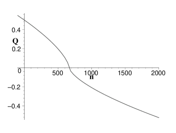
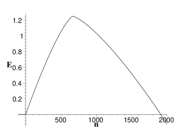
FIG. 6.: The evolution of the real part of the Ashtekar connection $Q$ and the triad $E$ for the discrete closed Friedmann model. The kink that is observed at the moment of maximum expansion corresponds to the fact that at that point the connection goes through zero and the discrete theory picks up two different parameterizations of the continuum theory at both sides of $Q=0$. It is therefore a coordinate feature. If one looks at the observables of the theory, they remain constant throughout evolution and nothing special happens at that point.

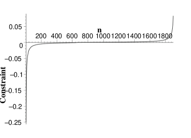
FIG. 7.: The continuum Hamiltonian constraint of the continuum theory written in the dimensionless form $1+(-Q^{2}+{1\over 4})/(|E|\Theta)$ evaluated on the discrete theory for the closed Friedmann model. The constraint is close to zero in the region of maximum expansion showing that the model achieves best approximation of the continuum theory in that region.

B Flat Friedmann model with $\Lambda=0$ and massless scalar field

This model will teach us about situations in which the continuum limit is not achieved as in the previous models.

The continuum Lagrangian is

$$L=E\dot{A}+\pi\dot{\phi}-N\left(-E^{2}A^{2}+\pi^{2}\right).$$ (81)

The equations of motion are straightforward. The model has two independent observables,

$$O_{1} = A\exp\left(\epsilon\phi\right),$$ (82)

$$O_{2} = E\exp\left(-\epsilon\phi\right),$$ (83)

and the obvious observable $\pi$ can be obtained from them as $\pi=\epsilon O_{1}O_{2}$, where $\epsilon=\pm 1$. Discretizing the action we get,

$$L=E_{n}\left(A_{n+1}-A_{n}\right)+\pi_{n}\left(\phi_{n+1}-\phi_{n}\right)-N_{n}\left(-E^{2}_{n}A_{n}^{2}+\pi_{n}\right).$$ (84)

Working out the equations of motion, the Lagrange multiplier gets determined to, (choosing $\epsilon=+1$),

$$N_{n}={1\over 2}{P^{\phi}_{n}-A_{n}P^{A}_{n}\over(P^{\phi}_{n})^{2}}.$$ (85)

The resulting equations of motion are,

$$P^{A}_{n+1} = {P^{\phi}_{n}\over A_{n}},$$ (86)

$$A_{n+1} = {A_{n}^{2}P^{A}_{n}\over P^{\phi}_{n}},$$ (87)

$$\phi_{n+1} = \phi_{n}+{P^{\phi}_{n}-A_{n}P^{A}_{n}\over P^{\phi}_{n}},$$ (88)

$$P^{\phi}_{n+1} = P^{\phi}_{n}.$$ (89)

Combining (86) and (87) one gets a recursion relation,

$${A_{n+1}\over A_{n}}={A_{n}\over A_{n-1}}=a.$$ (90)

Given initial values for $A_{0}$ and $A_{1}$, the solution to the recursion relation is immediate, stating that the ratio of two successive connections is a constant $a$. The solution is therefore of a power law form: $A_{n}=A_{0}a^{n}$, $P^{A}_{n}=P^{A}_{0}a^{-n}$.

Combining (86) and (88) we get,

$$\phi_{n+1}=\phi_{n}+1-a.$$ (91)

To recover a continuum limit we therefore need to take the limit $a\to 1$. Let us therefore consider $a=\exp(-\delta)$ with $\epsilon$ close to zero, we get $\phi_{n+1}-\phi_{n}=\delta$ and $\phi_{n}=\phi_{0}+n\delta$. If we obtain $\delta$ from this last expression and substitute it in the solution for $A_{n}$ we get $A_{n}=\exp(\phi_{n}-\phi_{0})A_{0}$. Therefore $A_{n}\exp(-\phi_{n})$ is a constant of the motion which reproduces the observable of the continuum theory (82). If one computes the normalized Hamiltonian constraint of the continuum theory evaluated on the discrete theory one gets,

$$1-{A_{n}P^{A}_{n}\over P^{\phi}_{n}}=\delta,$$ (92)

and indeed one recovers the continuum theory for $\delta\to 0$.

Notice that the continuum limit in this model arises in a very different way than in the previous model. There we had that for any initial data one asymptotically into the future reached a region that approximated well the continuum theory. The continuum limit was therefore an “attractor” in the dynamics of the theory. In this model one sees that the level of approximation of the continuum theory, as exhibited by the violation of the Hamiltonian constraint (92) is constant throughout the evolution. To achieve a certain level of accuracy one will have to choose the initial data such that the value of $\delta$ is the desired one.

This behavior however, has negative implications at the time of quantization. Since a quantum state is generically a superposition of many possible initial conditions, there will be no way of achieving a classical limit, unless one fine tunes the initial state carefully so only initial data that approximate the classical theory are included in the superposition. In the previous examples the universe generically behaved in a quantum way near the Big Bang and then became more classical into the future. In this model the universe will behave in the same fashion throughout the complete evolution, independent of time.

C The Bianchi cosmologies

We will not present a full discussion of Bianchi cosmologies, but will just mention some salient features in which some of the models resemble the behavior of the Friedmann models discussed before, and one situation in which they differ significantly.

The Bianchi cosmologies are spatially homogeneous space-times where the group of homogeneities acts transitively. If the structure constants of the algebra of symmetries are traceless, then one has the “Bianchi class A” models (Bianchi I, II, VIII, IX) . These models admit a straightforward Hamiltonian formulation as a reduction of the full action of general relativity via the symmetry. It is well known that the dynamics of these cosmological models classically is equivalent to a particle bouncing inside a potential well. In the case of the Bianchi IX and VIII the well is closed and the particle executes an infinite series of bounces against the walls. Each individual bounce can be approximated by a Bianchi type II solution and the motion of the particle between bounces can be approximated by a Bianchi type I solution. So basically by studying the Bianchi I and II models we capture approximately all the features needed to study the more complicated VIII and IX models. For this reason, and for simplicity we will restrict our attention to the I and II models.

The space-time metric of the Bianchi models can be written as,

$$ds^{2}=-dt^{2}+\sum_{i,j=1}^{3}g_{ij}\omega^{i}\omega^{j}$$ (93)

and for simplicity we will only consider diagonal models. The $\omega$’s are one forms that are invariant under the isometries. Following Misner [12] we introduce the following coordinatization of the three metric, $g_{ii}=\exp(2\beta^{i})$ and we define $\beta^{0},\beta^{+},\beta^{-}$ such that,

$$\beta^{1} = \bar{\beta}^{0}+\bar{\beta}^{+}+\sqrt{3}\bar{\beta}^{-},$$ (94)

$$\beta^{2} = \bar{\beta}^{0}+\bar{\beta}^{+}-\sqrt{3}\bar{\beta}^{-},$$ (95)

$$\beta^{3} = \bar{\beta}^{0}-2\bar{\beta}^{+}.$$ (96)

We then perform the coordinate transformation [13],

$$\beta^{0} = {\sqrt{3}\over 3}(2\bar{\beta}^{0}-\bar{\beta}^{+})$$ (97)

$$\beta^{+} = {\sqrt{3}\over 3}(-\bar{\beta}^{0}+2\bar{\beta}^{+})$$ (98)

$$\beta^{-} = \bar{\beta}^{-}.$$ (99)

In terms of these variables one can construct a canonical formulation for these models with action,

$$S=\int dt\left[p^{0}\dot{\beta^{0}}+p^{+}\dot{\beta^{+}}+p^{-}\dot{\beta^{-}}+N\left(-(p^{0})^{2}+(p^{+})^{2}+(p^{-})^{2}+U(\beta^{+},\beta^{-},\beta^{0})\right)\right].$$ (100)

For Bianchi I, $U(\beta^{+},\beta^{-},\beta^{0})=0$ and for Bianchi II, $U(\beta^{+},\beta^{-},\beta^{0})=12\exp(-4\sqrt{3}\beta^{+})$. The models therefore generically have a Hamiltonian constraint,

$$-(p^{0})^{2}+(p^{+})^{2}+(p^{-})^{2}+U(\beta^{+},\beta^{-},\beta^{0})=0.$$ (101)

In the case of the Bianchi I model, the constraint only depends on the canonical momenta and not on the coordinates. It is also known that there exists a canonical transformation that makes constraint only depend on the momenta in the Bianchi II model. If the constraint depends only on half of the canonical variables (either momenta or coordinates) the evolution equations preserve the constraints exactly and the Lagrange multipliers are not determined. This follows trivially from the fact that if one has $H(p^{i})=0$ the equation of motion following from the canonical transformation generating evolution include $p^{i}_{n+1}=p^{i}_{n}$ and the constraint is automatically preserved without fixing the Lagrange multipliers. Therefore one obtains a traditional discretization of the theory, unlike the ones we are discussing in this paper.

It is interesting to note that in both the Bianchi I and Bianchi II models one could choose variables where the constraint is both a function of coordinates and momenta. In the Bianchi I case the Ashtekar variables [14] are an example where this happens. In the Bianchi II case it happens in the variables we have been discussing. From these variables one can construct consistent discretizations that determine the Lagrange multipliers. This exhibits the type of ambiguities that one faces when discretizing a continuum model.

We will not present a complete discussion of the Bianchi II model, but we would like to highlight some features of interest. The discretized Lagrangian is,

$$L(n,n+1)=\sum_{a=0,+,-}p^{a}_{n}(\beta^{a}_{n+1}-\beta^{a}_{n})-N_{n}((p^{0})^{2}-(p^{+})^{2}-(p^{-})^{2})+12N_{n}\exp\left(-4\sqrt{3}\beta^{+}_{n}\right),$$ (102)

The resulting equations are,

$$P^{0}_{n+1} = P^{0}_{n}$$ (103)

$$P^{-}_{n+1} = P^{-}_{n}$$ (104)

$$P^{+}_{n+1} = \epsilon\sqrt{(P^{0}_{n})^{2}-(P^{-}_{n})^{2}-12\exp(-4\sqrt{3}\beta^{+}_{n})}\equiv\epsilon\sqrt{\Delta_{n}}$$ (105)

$$\beta^{-}_{n+1} = \beta^{-}_{n}-N_{n}P^{-}_{n+1}$$ (106)

$$\beta^{0}_{n+1} = \beta^{0}_{n}+N_{n}P^{0}_{n+1}$$ (107)

$$\beta^{+}_{n+1} = \beta^{+}_{n}-N_{n}P^{+}_{n+1}$$ (108)

$$N_{n} = {P^{+}_{n}-P^{+}_{n+1}\over 24\sqrt{3}\exp(-4\sqrt{3}\beta^{+}_{n})}$$ (109)

where as before one first has to define variables canonically conjugate to $\beta^{+},p^{+}$, etc. We have written the equations replacing the momenta canonically conjugate to $\beta$ and relabeled $p^{0}_{n}$ as $P^{0}_{n+1}$. We have also solved the constraint for the Lagrange multiplier in the last equation.

We choose $\epsilon=-1$ and start with initial data at $n=0$ such that $\Delta_{0}>0$ and $N_{0}>0$, $P^{0}_{0}>0$. Examining the discrete equations, one can see that the system starts with expanding $\beta^{0}$ and $\beta^{+}$. $\beta^{-}$ can either grow or decrease. One can also see that $\Delta_{n}>0$ and $N_{n}>0$ for all $n$. That is, the solution expands indefinitely. If one chose $\epsilon=1$ and $\Delta_{0}>0$ and $N_{0}>0$, $P^{0}_{0}<0$, then the universe starts by contracting in $\beta^{0}$, expanding in $\beta^{+}$. The expansion continues indefinitely without changes of signs in the variables. Checking the expression of the three-volume $V_{n}=\exp(\sqrt{3}[2\beta^{0}_{n}+\beta^{+}_{n}])$, one can see that the volume goes to zero at $n\to\infty$. Therefore the discrete theory has a singularity. Notice that the unavoidability of the singularity in the discrete theory is related to the fact that in the continuum the singularity is at the edge of the domain, therefore it will always be present if one discretizes. One could have chosen a set of variables in which the singularity occurs in a point interior to the domain (for instance, the usual metric variables with appropriate time parameterization) and then the discrete theory could have avoided the singularity as in previous models we considered. Notice that it is not guaranteed that having the singularity within the domain will avoid the singularity. Essentially what has to happen for the singularity to be present in the discrete theory is that it happens at an accumulation point of grid points, therefore the discrete theory cannot “walk over” the singularity.

To show that this is actually possible for this model, let us consider the following canonical transformation [13],

$$\tilde{P}^{+}_{n} = \sqrt{(P^{+}_{n})^{2}+12\exp(-4\sqrt{3}\beta^{+}_{n})},$$ (110)

$$\tilde{\beta}^{+}_{n} = {\sqrt{3}\over 6}\left\{\left[-P^{+}_{n}+\sqrt{(P^{+}_{n})^{2}+12\exp(-4\sqrt{3}\beta^{+}_{n})}\right]-\log\left(2\sqrt{3}\exp(-2\sqrt{3}\beta^{+}_{n})\right)\right\}.$$ (111)

The action now reads,

$$S=\int dt\left[p^{0}\dot{\beta^{0}}+p^{+}\dot{\tilde{\beta}^{+}}+p^{-}\dot{\beta^{-}}+N\left(-(p^{0})^{2}+(\tilde{p}^{+})^{2}+(p^{-})^{2}\right)\right].$$ (112)

This action, which has a constraint that is only a function of the momenta, is an example of the ambiguities present when constructing the discrete theory. If one discretizes this form of the action, the Lagrange multiplier $N$ is not determined by the discrete equations and the discrete theory has a completely different nature than the ones we have considered before. These kinds of ambiguities are unavoidable, it is well known that infinitely many discrete theories can approximate the same continuum theory.

Let us now consider the canonical transformation generated by $F_{2}=\exp(\beta^{0})p^{T}$, such that the new coordinate $T=\exp(\beta^{0})$ and $p^{0}=TP^{T}$. In terms of the variables $(T,\beta_{\pm})$ and their conjugate momenta $(p^{T},p^{\pm})$ the action now reads,

$$S=\int dt\left[p^{T}\dot{T}+p^{+}\dot{\tilde{\beta}^{+}}+p^{-}\dot{\beta^{-}}+N\left(-T^{2}(p^{T})^{2}+(\tilde{p}^{+})^{2}+(p^{-})^{2}\right)\right].$$ (113)

The resulting theory, upon discretization exhibits the same behavior as the Friedmann model with $m=0$ we discussed before, in particular $T_{n+1}=aT_{n}$ with $a$ a constant. If $a$ is large enough the universe (run backwards) at some point departs significantly from the continuum behavior and instead of contracting, starts to expand, thus avoiding the singularity, as in the case of the Friedmann model.

Summarizing, we see that the behavior of the Bianchi models is similar to the behavior of the Friedmann models we discussed in the previous section. It would be interesting to study the Bianchi models using Ashtekar’s new variables. Such variables have several attractive features. The singularity happens within the domain, so it is likely to be avoided in the discrete theory, as it was in the case of the Friedmann model with $\Lambda$ and a very massive scalar field.

V Conclusions

We have studied the recently introduced “consistent discretization” approach to general relativity in the case of cosmological models. This helps to clarify, through examples, several questions that can be raised concerning that approach. First and foremost, the unusual property of having the Lagrange multipliers determined operates without difficulty in the models considered. We never encounter that the equations imply that the lapse is complex or that it is multi-valued during evolution. Moreover, the issue of how the discrete theory achieves a continuum limit is illuminated. We see that the possibility of having a continuum limit depends on the type of model and of discretization chosen. Some models exhibit continuum behavior spontaneously as an attractor in a region of their evolution. In other models, careful tuning of initial data is needed to approximate the continuum theory. The Big Bang singularity can be avoided in a generic fashion in some models, whereas in others it appears as inevitable, and this can be forecasted from the way the singularity appears in the continuum theory. We also saw explicitly how different formulations of the continuum theory can, upon discretization, exhibit radically different behaviors at the level of the discrete theory. Finally, the quantization of the discrete theory, in spit of the fact that the latter has no constraints, is non-trivial. One discovers that the discrete theories have remnant symmetries that imply the existence of constants of the motion that are remnants of the observables (“perennials”) of the continuum theory. This opens several possibilities for the quantization, relating to how one approaches the “problem of time”. One can attempt a straightforward Schrödinger quantization of the theory, but the evolution one obtains is in terms of a “time” that has no physical meaning. One can attempt to “gauge fix” the remnant symmetry and one obtains a theory with a physically well motivated time that can be quantized a la Schrödinger, but it has the drawback that one has artificially decided to treat a variable as classical, even in regimes in which it should not be. Finally, one can attempt a relational introduction of the notion of time that is free of the many problems that plagued such attempts in the continuum theory and therefore provides a natural solution to the problem of time in quantum cosmology.

It is clear that one can only take the examples presented in this paper, given their simplicity, as first attempts to understand this approach to discrete general relativity. Further work will be needed to gain confidence that the approach can be used in more realistic settings. But already the exploration of this simple models has been a useful laboratory to exhibit the kind of behaviors that one may encounter in the discretized theories.

- [1] R. Loll, Living Rev. Rel. 1, 13 (1998).
- [2] C. Di Bartolo, R. Gambini, J. Pullin, Classical and Quantum Gravity 19, 5475 (2002); R. Gambini, J. Pullin, gr-qc/0206055 to appear in Phys. Rev. Lett.
- [3] T. D. Lee, in “How far are we from the gauge forces” Antonio Zichichi, ed. Plenum Press, (1985)
- [4] H. Kodama, Phys. Rev. D 42, 2548 (1990).
- [5] L. Smolin “The life of the cosmos”, Oxford University Press (1999).
- [6] P. A. M. Dirac, Z. Phys. Sow. Band 3, Heft 1 (1933), reprinted in “Selected Papers on Quantum Electrodynamics”, J. Schwinger, ed., Dover, New York (1958); see also P. Ramond “Field Theory: A Modern Primer”, Benjamin/Cummings, Reading, MA (1981) p 72.
- [7] K. Kuchař, “Time and interpretations of quantum gravity”, in “Proceedings of the 4th Canadian conference on general relativity and relativistic astrophysics”, G. Kunstatter, D. Vincent, J. Williams (editors), World Scientific, Singapore (1992).
- [8] M. Bojowald Phys. Rev. Lett. 87, 121301 (2001).
- [9] B. S. Dewitt, Phys. Rev. 160, 1113 (1967).
- [10] D. N. Page and W. K. Wootters, Phys. Rev. D 27, 2885 (1983); W. Wooters, Int. J. Theor. Phys. 23, 701 (1984); D. N. Page, “Clock time and entropy” in “Physical origins of time asymmetry”, J. Halliwell, J. Perez-Mercader, W. Zurek (editors), Cambridge University Press, Cambridge UK, (1992).
- [11] R. Gambini, R. Porto, J. Pullin, in preparation.
- [12] C. Misner, in “Magic without magic”, J. Klauder (editor), Freeman, San Francisco (1972).
- [13] A. Ashtekar, R. Tate and C. Uggla, Int. J. Mod. Phys. D 2, 15 (1993).
- [14] H. Kodama, Prog. Theor. Phys. 80, 1024 (1988); A. Ashtekar and J. Pullin, Ann. Isr. Phys. Soc. 9, 65 (1990).