Critical behavior of gravitating sphalerons
Abstract
We examine the gravitational collapse of sphaleron type configurations in Einstein–Yang–Mills–Higgs theory. Working in spherical symmetry, we investigate the critical behavior in this model. We provide evidence that for various initial configurations, there can be three different critical transitions between possible endstates with different critical solutions sitting on the threshold between these outcomes. In addition, we show that within the dispersive and black hole regimes, there are new possible endstates, namely a stable, regular sphaleron and a stable, hairy black hole.
I Introduction
Over the last two decades, substantial effort has been brought to bear on the study of gravitating Yang–Mills fields. This research has resulted in the discovery of numerous solutions to the coupled Einstein–Yang–Mills(–Higgs and/or –dilaton) equations. These solutions include both black hole and regular or particle–like solutions. In addition to confirming the richness of these nonlinear systems, this work has also been helpful in clarifying the standing of the black hole uniqueness theorems and various “no-hair” ideas.
While many of these solutions have been found by solving the appropriate static equations, it was realized early on that understanding the stability of these solutions is important in order to ascribe relative significance to these solutions within the context of some of the no–hair conjectures. The primary means for evaluating stability have been linear perturbation analyses of various static solutions. As a result, many of these static, gravitating Yang–Mills(–scalar) configurations have been found to be unstable to small time–dependent perturbations.
That many of these solutions appear unstable in linear perturbation theory does not necessarily mean that such solutions are without significance. Indeed, it is now widely accepted within the context of gravitational critical phenomena that some of these solutions will have relevance as attractors in the critical collapse of gravitating fields at the threshold of black hole formation [1, 2]. As an example, the Bartnik–McKinnon solutions of the spherically symmetric, static Einstein–Yang–Mills equations are a countably infinite family of regular solutions characterized by the integer number, , of zero–crossings of the gauge potential. These solutions are unstable in linear perturbation theory with the member of the family having unstable modes.‡‡‡Strictly, this is true if only the radial, gravitational perturbations are excited. If additional components of the gauge potential are also perturbed (i.e. the sphaleron sector), the solution will have unstable modes, the sphaleron sector contributing an additional unstable modes to those from the gravitational sector.[3] Thus, the member of this family has a single unstable mode and is a candidate for being a critical solution in the gravitational collapse of a pure Yang–Mills field. Indeed, this is exactly the result found in [4] where the full evolution equations for the model were solved. The Bartnik–McKinnon solution is the critical solution that sits on the threshold between the complete dispersal of the collapsing field and the formation of a finite size black hole (Type I collapse). The value of the unstable mode for this solution then correctly predicts the scaling relation for the lifetime of near–critical solutions.
In addition to these regular solutions, the Einstein–Yang–Mills equations also admit another countably infinite family of solutions, but with a nonzero horizon. These black hole solutions have non-trivial hair outside their horizons and are again characterized by the number, , of zero-crossings of the gauge potential. They too are unstable in linear perturbation theory with unstable modes from the gravitational sector. In agreement with expectations, it has been shown that the solution is also a critical solution [5]. But this non-abelian or colored black hole solution, rather than separating dispersion and black hole formation as does the Bartnik–McKinnon solution, sits on the threshold between two different kinds of dynamical collapse.
Given this behavior, it is natural to conjecture that other configurations of gravitating Yang–Mills fields should likewise exhibit critical phenomena. With that in mind, we consider here the nonlinear evolution of gravitating sphalerons in Einstein–Yang–Mills–Higgs theory. We provide evidence that there can be three critical transitions in the initial data space. These include the now standard Type I and Type II transitions as well as the transition mentioned above between different kinds of dynamical collapse on which sits a colored or “hairy” black hole as the intermediate attractor. In the process of examining critical gravitational collapse within this system and the formation of such “hairy” black holes as attractors in the black hole regime, we have also confirmed the stability of two additional endstates of collapse. One is a regular, gravitationally bound configuration of Yang–Mills–Higgs field forming a stable “sphaleron star.” The second is a family of stable, hairy black holes different from those that serve as the critical solutions in the black hole regime. The existence of such stable solutions appears to have first been predicted by Maison [6].
The outline of the remainder of the paper is then as follows. Section 2 summarizes the equations which constitute the full evolution problem and our numerical approach to their solution. Section 3 describes the numerical results, including results of our parameter space searches, the critical solutions and the nature of the stable solutions. Section 4 offers some conclusions and thoughts for future directions.
II The model
Our starting point in studying the gravitational collapse of configurations of Yang–Mills–Higgs fields is the action
| (1) |
where is the Yang-Mills field strength tensor given by
| (2) |
is the gauge covariant derivative whose action on the Higgs doublet, , is
| (3) |
and the potential is taken to be
| (4) |
Varying the action with respect to the metric, the field strength and the Higgs field result in the Einstein equations and the curved space Yang-Mills and Higgs equations, respectively. These are
| (6) | |||||
| (7) | |||||
| (8) |
With these general forms for the equations of motion, we make some simplifying assumptions. In particular, we will restrict ourselves to spherically symmetric gravitational collapse and work exclusively with an gauge group. We also make the assumption that the Higgs field lives in the fundamental representation of . The corresponding flat space version of this theory includes the so–called sphaleron solutions [7].
Our intent is to solve the full set of nonlinear, evolution equations representing gravitational collapse. In order to do this numerically we must fix both the coordinate freedom and the gauge freedom in our model. There are, of course, numerous possibilities, but we will try to hew fairly closely to related work of others in the field. For the coordinate system, we will work in maximal, areal coordinates. If the general form of the spherically symmetric metric is written as
| (9) |
where the metric components depend only on and , the choice of areal coordinates amounts to while choosing maximal time slices corresponds to the vanishing of the trace of the extrinsic curvature, .
For the Yang-Mills field, the most general form for a spherically symmetric gauge potential is the Witten ansatz [8]:
| (10) |
where the () are the spherical projection of the Pauli spin matrices and form an anti-Hermitian basis for the group satisfying . With this ansatz for the gauge potential there is some gauge freedom that allows us to simplify its form, namely the potential is invariant under a transformation of the form . We can fix some of that gauge freedom by choosing . This choice effectively eliminates the dependance in the above gauge transformation. If we choose to work within the so-called “magnetic ansatz” we can fix the remaining freedom in the following way. It can be shown that in this ansatz, the component is a function only of , i.e. it is now pure gauge and can be set to zero as part of our gauge fixing. The remaining fields, and , under the remaining constant gauge transformations are merely sent into linear combinations of each other and hence we can fix the last bit of gauge freedom by setting . This leaves as the sole non-zero component of the gauge potential.
Our form for the Higgs field, taken from [9], is
| (11) |
and though not strictly spherically symmetric, results in a spherically symmetric energy density [6]. We will consider in this work only the case in which . This is not a gauge choice but an additional assumption made merely to simplify the resulting equations and dynamics. A similar thing is done, for instance, in [9].
With these assumptions, the evolution equations for the Yang-Mills field become
| (12) | |||||
| (13) | |||||
| (14) |
while the evolution equations for the Higgs field are given as
| (15) | |||||
| (16) | |||||
| (17) |
where, as usual, overdots and primes denote differentiation with respect to and respectively. Both of these sets of evolution equations are supplemented with the first order definitions and as well as the constraints on the metric components coming from the Einstein equations
| (18) | |||||
| (19) | |||||
| (20) | |||||
| (21) |
The matter stress-energy terms in these equations are given by
| (22) | |||||
| (23) | |||||
| (24) | |||||
| (25) |
Boundary conditions are implemented by demanding regularity at the origin and requiring the presence of only outgoing radiation at large distances (see [5]). The resulting constraints on the metric components require . The matter fields may satisfy one of two possible regular configurations at the origin. Either, and , or and . These two choices correspond to the odd and even node solutions, respectively [9]. In order to find the critical solution we choose the former and look for the solution with a single unstable mode. The outgoing conditions require that at the edge of our grid,
| (26) | |||||
| (27) | |||||
| (28) | |||||
| (29) |
For the initial pulse, we use a “time-symmetric kink” as in [5] for the gauge potential, namely
| (30) | |||||
| (31) |
where the parameters and are chosen so and . The parameters and are the center and width of the kink, respectively.
The Higgs field is initialized as
| (32) | |||||
| (33) |
where the parameter is usually set to . This is primarily due to the fact that varying does not significantly change the final result of the collapse. As a consequence, we perturb the Higgs field via a gaussian pulse. Similar to the initialization for the Yang–Mills field, the parameters , , and which describe the initialization of the Higgs field represent the amplitude, center, and width of the gaussian pulse, respectively. These initial data parameters for the Yang–Mills and Higgs fields will constitute our initial data set and will be used when tuning our evolutions to the critical solutions.
Our numerical approach closely follows that of [5]. We use a uniform grid recognizing that we will not have sufficient resolution to investigate Type II collapse in a completely satisfactory way. Nonetheless, we have indications verifying the existence of Type II behavior in our model. For this paper, therefore, we focus our primary interest on the black hole transition and the dynamics occuring within the black hole regime.
We use an iterative Crank–Nicholson scheme for the evolution equations while for the constraints, we simply integrate outward from the origin. As we want to consider evolutions that extend to the future of black hole formation, our use of maximal slicing is crucial. In our coordinates, the apparent horizon equation is an algebraic relation
| (34) |
We use the same black hole excision technique developed in [10] and used in [5]. As discussed there, we set a threshold value slightly larger than one such that if exceeds that value for certain grid points, we discard those points at future time steps considering them inside the apparent horizon. At the boundary of this region, we need no new boundary conditions for the evolution equations. For those variables solved via constraint equations we either switch to solving an evolution equation subsequent to the formation of a horizon or we “freeze” the variable (e.g. ) such that it retains the value it had when the horizon formed [5]. As a result, though we can observe matter falling into the horizon, we cannot comment on any dynamics within the apparent horizon as the evolution is effectively frozen for values of the radial coordinate less than the horizon radius. This procedure thus allows us to evolve past the formation of the black hole and thereby investigate such things as the final endstates as well as the critical dynamics in the vicinity of transition regions.
We have tested the resulting code and shown it to be second–order convergent and to conserve mass. It also reproduces the results of [5] in the limit that the Higgs field and its coupling vanish. Finally, we note that we made extensive use of RNPL (Rapid Numerical Prototyping Language) [11], a language written expressly to aid the differencing and solution of PDE’s.
III Results
In attempting to evolve these equations, it quickly became clear that the size of the initial data sets that could be varied is somewhat unwieldy and we had to make choices in order to restrict the possible sets of initial data parameters. Although we have performed numerous evolutions by varying the elements of different sets of initial data parameters, we will focus on the evolution of two sets of parameters to highlight our results. Other sets would appear to give qualitatively similar conclusions. When we evolve these equations, we confirm many of the same aspects that have come to be expected in similar models. However, there are, at the same time, a number of unexpected surprises.
To begin our examination of the dynamics of this model, we consider varying two parameters describing the initialization of the gauge potential, namely and , the center and width of the kink, respectively. The amplitude of the perturbing, gaussian pulse for the Higgs field is set to zero, , and the width of the function describing the Higgs is . We call this configuration the “bland” Higgs field. Note that in this section, all the pictured results are for values of the Higgs coupling parameters, and .
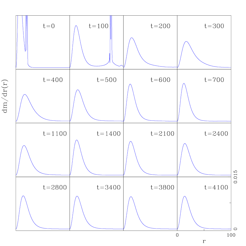
On varying the center and width of the Yang-Mills potential, , one finds three distinct regions of the initial data space. These correspond, as in [5], to generalized Type I collapse, generalized Type II collapse and a “dispersive” region in which no black hole forms. On the boundaries between these regions sit appropriate critical solutions. It is worth noting, however, that in the region in which no black hole forms, we no longer observe the complete dispersal of all the matter fields. Instead, while a majority of the fields do escape to infinity, a nontrivial portion of the fields forms a bound state, or “sphaleron star.” Shortly after formation, this solution oscillates rapidly, but settles down to what appears to be a static solution. Long evolutions with confirm the stability of this solution. The mass of this stable star is, to within a few percent, independent of any of the initial field parameters. The solution and its mass do appear to depend on the coupling parameters and [6]. Snapshots of a typical evolution in the “dispersive” regime are shown in Figure 1.
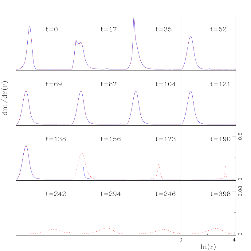
In the region with generalized Type I collapse, we note no significant change in the dynamics from those similarly exhibited in [5]. The collapsing matter forms a black hole with finite mass which, after the residual fields have dispersed to infinity, settles down to the Schwarzschild solution. On the Type I critical line separating black hole formation and the sphaleron star configuration, we find a regular sphaleron as the critical solution analogous to the Bartnik–McKinnon solution. An example of the critical behavior at this Type I transition is given in Figure 2 in which a sub–critical and a super–critical evolution are shown.
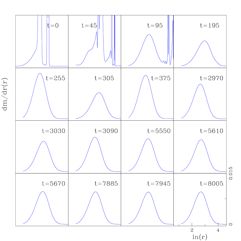
Within the generalized Type II region, there are some new features. As in [5], this region is again characterized by the dynamical formation of a black hole with finite mass. As the critical line which separates dispersion (or strictly, sphaleron star formation) from the black hole region is approached, the mass of these black holes begins to decrease such that we interpret the critical transition as Type II. However, the black holes that form away from the critical line after the transient hair has dispersed to infinity do not settle down to Schwarzschild black holes. Instead, the final endstate would appear to be a stable, colored black hole with non–trivial Yang–Mills and Higgs fields outside the event horizon. This, of course, is analogous to the sphaleron star that forms in the no–black–hole region of this system rather than the complete dispersal of the fields seen in [5]. The basic dynamics in this case are illustrated in Figure 3. The collapsing configuration forms a finite mass black hole with a significant portion of the remaining field escaping to infinity. Nevertheless, some of the hair remains behind and within the vicinity of the event horizon. This hair oscillates for some time and eventually settles down to a stable configuration. Evolutions on the order of show no appreciable diminution or instability in the fields.
The mass of the hair in these black hole solutions also seems to be independent of the initial data parameters. Though the radius of the black hole will vary with the initial parameters, the exterior mass remains unchanged. This observation is consistent with and similar to that for the sphaleron stars in which a single stable, regular solution is found throughout the no–black–hole region. In addition, like their regular counterparts, the black hole solutions will depend on the parameters and . Curiously, the mass of this exterior hair is very nearly the same value as the mass of the sphaleron star. Thus, in one sense, these hairy black hole solutions can be thought of as sphaleron star solutions within which the central density increases to the point that a horizon forms. This is similar in turn to gravitating t’Hooft-Polyakov monopoles. For certain values of the coupling, the monopoles can have a black hole form at their center.
For the solutions near the threshold separating black hole formation and dispersion, we find hints that these are indeed Type II critical solutions and that the black hole mass scales as expected. However, we stress again that our unigrid code is not able to settle this issue definitively and that it awaits additional study.
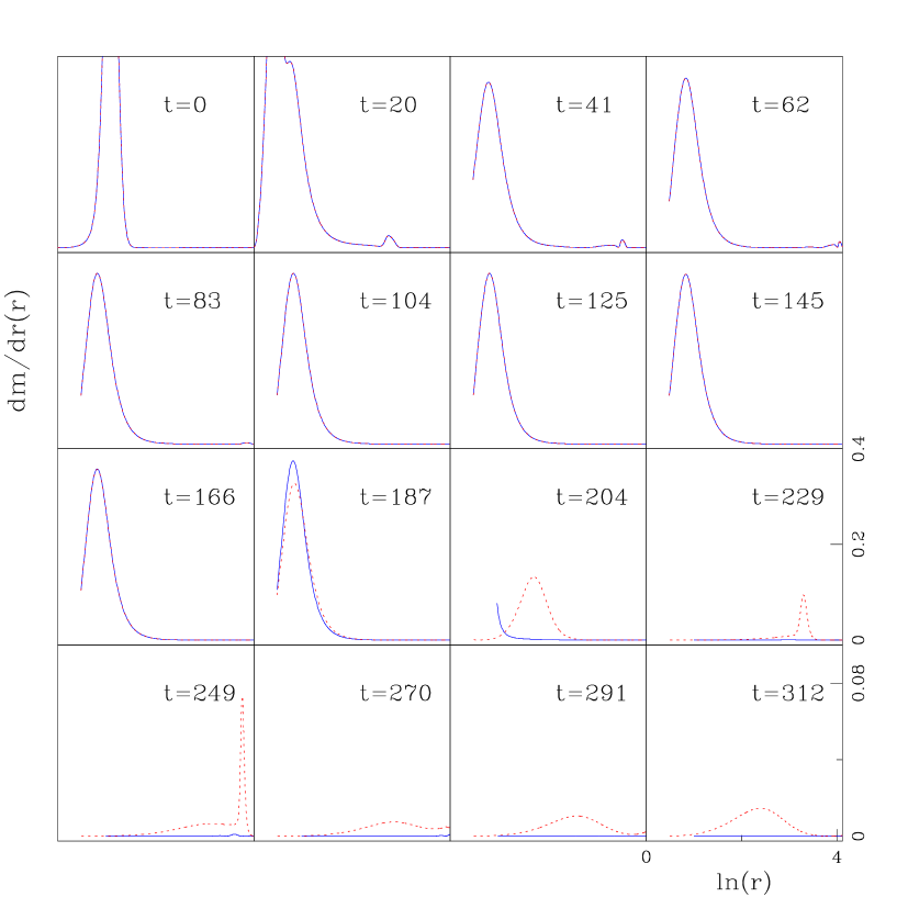
We are able, though, to consider the transition between the different types of dynamical collapse in the black hole regime. Again, we find a family of critical solutions separating generalized Type I collapse from generalized Type II collapse. These critical solutions are themselves sphaleron black holes parameterized by their horizon radius such that as one moves away from the “triple point” in Figure 5, that radius increases. On the Type II side of this line, near–critical evolutions have dynamics described above with the collapsing configuration forming a black hole of finite mass with non–trivial hair outside. However, as the transition between Type II and Type I is approached, there is an intermediate solution – a hairy black hole – which forms and to which the evolving solution is attracted. This intermediate solution is unstable and eventually collapses. For initial configurations on the Type II side, the collapse is distinctive in that very little of the exterior fields falls into the black hole. Rather, some of it is dispersed to infinity while the remainder reconstitutes in a new and different colored configuration outside the black hole already present. This is shown in Figure 3 for a generic collapse in the Type II regime as well as in the last frames of Figure 4 for a near–critical evolution.
On the Type I side of the critical line, similar near–critical evolutions exhibit the same early time dynamics with the formation of a finite mass black hole and the approach to the intermediate hairy black hole. However, as the critical line is approached, this unstable black hole now collapses and loses most of its hair into the black hole causing it to grow in size. A picture of both collapse dynamics is shown in Figure 4.
So far, our entire description has been within the context of varying two of the initial data parameters that describe the Yang–Mills field. We have chosen to vary the center and width of the Yang–Mills kink, but the same results hold for other Yang–Mills parameters. However, there does appear to be a non–trivial difference in our description of the initial data space if we include a parameter of the Higgs field in the set of two parameters which we vary in order to search for critical behavior.
In the original, so-called “bland” Higgs case, the structure of the phase space is very similar to that found in [5], namely Type I and II critical collapse separated by the previously discussed colored, critical solution. This is shown in Figure 5.
However, in the event that we turn on the exponential, perturbing pulse for the Higgs field, and look at the phase space including one Yang–Mills parameter and one Higgs parameter, we see a different picture, shown in Figure 6. In this case and for the region of the parameter space explored, there appears to be no critical boundary between Type I collapse and the formation of a sphaleron star. Instead, Type II collapse would seem to border the region in which the regular solution is formed. It would therefore seem that in this region of the initial data space, there is no “triple point.” One might have imagined that as one varied the amplitude of the exponential portion of the Higgs pulse that there would be such a point in each plane for a given . However, this does not seem to be the case and is an issue deserving of more investigation.
Finally, we note that the critical solutions separating the two types of collapse and Type I collapse from sphaleron star formation exhibit time scaling as would be expected. As the single, unstable mode characteristic of each critical solution is tuned out, near–critical solutions spend increasing amounts of time as measured by an asymptotic observer on the critical solution. These scaling relations are given by where is the characteristic time scale for the collapse of the unstable critical solution. It corresponds to the inverse Lyapounov exponent of the unstable mode. Such scaling relations specific to points on the relevant critical lines are shown in Figures 8 and 7.
IV Discussion
We have presented evidence for critical phenomena in the gravitational collapse of sphaleron configurations of Yang–Mills–Higgs fields. In many respects, this collapse is qualitatively similar to that in the Einstein–Yang–Mills system but does have some notable suprises. The critical behavior is seen again in three possible transitions. On each of these transitions sit critical solutions which serve as intermediate attractors for nearby evolutions in the initial data space. Near the critical line separating Type I collapse from the regular solution as well as for the critical line separating the two types of dynamical black hole formation, there are time scaling relations as the near–critical solutions approach the critical solutions. In addition, the mass of the black holes formed in the appropriate region will exhibit a mass gap in crossing these critical lines. Near the critical line separating Type II collapse from the regular endstate region, we have indications that the mass of the black hole scales without a mass gap, but again, due to our unigrid code, we can not settle this conclusively although expectations and indications would bear this out.
Among the surprises in this model are that in certain regions of the initial data space, we find that regular, stable, sphaleron solutions are produced rather than the purely dispersive regime seen in [5]. However, we also have stable, hairy or colored black holes produced in the supercritical, black hole regime. This contrasts again with earlier results in which the endstate in spherical symmetry was always a Schwarzschild black hole. Thus, the transition here between generalized Type I and Type II collapse is a transition between different types of black holes. Within the Type I region, the endstate is always a Schwarzschild black hole with the exterior gauge and Higgs fields either falling into the existing black hole or dispersing to infinity. In the Type II region, the final black holes are stable, colored black holes. It is worth reemphasizing that the colored black hole solutions sitting on the critical line separating types of black hole collapse are not the same as the stable, colored black holes that are the final endstates in the Type II region. This can be seen most easily in Figure 4.
It is also noteworthy that the existence of all the solutions which we find is contingent on the magnetic ansatz within which we have chosen to work. In general, both the regular and colored black hole solutions which we find to be stable endstates of collapse are expected to be unstable based on a linear perturbation analysis [12]. However, such an analysis assumes that both the gravitational and sphaleron sectors in the theory are perturbed. Our evolutions perturb only the gravitational sector. It is reasonable to assume that the stable solutions which we find will become unstable on perturbation of the Yang–Mills gauge field away from the magnetic ansatz. We hope to address this issue in future work.
Another issue for future consideration is the structure of the initial data space. A curiosity of our current results is that the “triple point” would seem to disappear as the Higgs field is varied. As a result, the boundary between regular endstates (sphaleron star formation here) and black hole formation is taken up entirely by a Type II transition.
Nonetheless, given the structure of the initial data space, one can draw an analogy with the gravitating monopole case in which a small black hole can form within a t’Hooft-Polyakov monopole coupled to gravity. This stable object can be rendered unstable above a maximum value of the horizon radius at which point the exterior Yang-Mills-Higgs hair will either fall into the black hole or disperse leaving a final Schwarzschild black hole. A similar thing happens in the current sphaleron case. For example, following a line of constant in Figure 5 that intersects each region we see that as decreases, one can interpret the process in a similar way. A regular solution develops a small, stable black hole at the center which (with decreasing width of the initial Yang-Mills potential, ) increases in size until the combined sphaleron and black hole system becomes unstable and is replaced with a larger Schwarzschild black hole. As a result, it would be interesting to consider the full dynamical evolution of the gravitating monopole and compare with the sphaleron case reported here.
Acknowledgements
This research has been supported in part by NSF grants PHY-9900644 and PHY-0139782. EWH would like to thank A. Wang for useful discussions as well as M. Choptuik and R. Marsa for their work on an earlier code which served as the precursor to the one described here.
REFERENCES
- [1] M. W. Choptuik, Phys. Rev. Let. 70, 9 (1993).
- [2] C. Gundlach, Living Rev. Rel. 2, 4 (1999).
- [3] G. Lavrelashvili and D. Maison, Phys. Lett. B349, 438 (1995); M .S. Volkov, O. Brodbeck, G. Lavrelashvili, and N. Straumann, Phys. Lett. B349, 438–442, (1995).
- [4] M.W. Choptuik, T. Chmaj, P. Bizon, Phys. Rev. Let. 77, 424-427 (1996).
- [5] M. W. Choptuik, E. W. Hirschmann, R. L. Marsa, Phys. Rev. D 60, 124011 (1999).
- [6] D. Maison, “Solitons of the Einstein–Yang–Mills theory,” gr-qc/9605053 (1996).
- [7] R.F. Dashen, B. Hasslacher, A. Neveu, Phys Rev D10, 4138 (1974)
- [8] E. Witten, Phys. Rev. Lett. 38, 121 (1977).
- [9] B. R. Greene, S. D. Mathur, C. M. O’Neill, Phys. Rev. D 47, 2242 (1993).
- [10] R. L. Marsa and M. W. Choptuik, Phys. Rev. D 54, 4929 (1996).
-
[11]
R.L. Marsa and M.W. Choptuik, “The RNPL User’s Guide”,
http://laplace.physics.ubc.ca/People/marsa/rnpl/users_guide/users_guide.html (1995);
Software available from http://laplace.physics.ubc.ca/Members/matt/Rnpl/index.html - [12] P. Boschung, O. Brodbeck, F. Moser, N. Straumann, M. Volkov Phys. Rev. D 50, 3842-3846 (1994).