We describe recent progress in the numerical study of the structure of rapidly rotating superfluid neutron star models in full general relativity. The superfluid neutron star is described by a model of two interpenetrating and interacting fluids, one representing the superfluid neutrons and the second consisting of the remaining charged particles (protons, electrons, muons). We consider general stationary configurations where the two fluids can have different rotation rates around a common rotation axis. The previously discovered existence of configurations with one fluid in a prolate shape is confirmed.

1 Introduction

Most current studies of neutron star oscillations are based on a simple perfect fluid model for a neutron star, which neglects (besides other things like the magnetic field, crust etc.) the crucial importance of superfluidity. The presence of substantial amounts of superfluid matter in neutron stars is backed by a number of theoretical calculations of the state of matter at these extreme densities (e.g. see [1, 2]), and by the qualitative success of superfluid models to accommodate observed features of glitches and their relaxation (e.g. see [3] and references therein). For both the study of oscillation modes of superfluid neutron stars, and the modelling of the particular glitch instability, it is important to know the (quasi-) stationary initial state of the unperturbed neutron star. The principal difference with ordinary-fluid models consists of the fact that in a superfluid model there are two fluids (i.e. the superfluid neutrons and all the rest), that can flow independently. As a result of the slow spindown process of the neutron star, the neutron superfluid will lag behind the charged constituents, due to its complete absence of viscosity. The generic configuration therefore corresponds to a (quasi-) stationary two-fluid model, with the two (strongly coupled!) fluids rotating around the same axis, but with different rotation rates. This model has been studied before in both the Newtonian ([4, 5]) and the relativistic framework [6], using the slow-rotating approximation and a simple “polytropic” two-fluid equation of state. Here we describe a fully relativistic numerical approach to solve the problem for arbitrary rotation rates.

2 The two-fluid model

We briefly present the notation and formalism used to describe the two-fluid model for superfluid neutron stars, a more detailed discussion can be found in [7, 8]. We consider two fluids, representing the neutrons (denoted by the label $\mathrm{n}$) and the remaining charged components (denoted by $\mathrm{c}$) respectively. Superfluidity allows the neutrons to flow independently of the remaining constituents, without any direct frictional force between the neutrons and the second fluid. Another implication of superfluidity is that the rotating neutron fluid will be threaded by a lattice of microscopic quantized vortices, but their effect on the macroscopic scale is neglected here, so we treat the neutrons simply as an inviscid fluid. The kinematics of the two fluids is described by the respective rest-frame particle number densities $n_{\mathrm{n}}$ and $n_{\mathrm{c}}$, together with the four-velocities $\textstyle u_{\mathrm{n}}$ and $\textstyle u_{\mathrm{c}}$. The corresponding particle four-currents are therefore $\mathchoice{\mbox{\boldmath$\displaystyle n_{\mathrm{n}}$}}{\mbox{\boldmath$\textstyle n_{\mathrm{n}}$}}{\mbox{\boldmath$\scriptstyle n_{\mathrm{n}}$}}{\mbox{\boldmath$\scriptscriptstyle n_{\mathrm{n}}$}}=n_{\mathrm{n}}\mathchoice{\mbox{\boldmath$\displaystyle u_{\mathrm{n}}$}}{\mbox{\boldmath$\textstyle u_{\mathrm{n}}$}}{\mbox{\boldmath$\scriptstyle u_{\mathrm{n}}$}}{\mbox{\boldmath$\scriptscriptstyle u_{\mathrm{n}}$}}$ and $\mathchoice{\mbox{\boldmath$\displaystyle n_{\mathrm{c}}$}}{\mbox{\boldmath$\textstyle n_{\mathrm{c}}$}}{\mbox{\boldmath$\scriptstyle n_{\mathrm{c}}$}}{\mbox{\boldmath$\scriptscriptstyle n_{\mathrm{c}}$}}=n_{\mathrm{c}}\mathchoice{\mbox{\boldmath$\displaystyle u_{\mathrm{c}}$}}{\mbox{\boldmath$\textstyle u_{\mathrm{c}}$}}{\mbox{\boldmath$\scriptstyle u_{\mathrm{c}}$}}{\mbox{\boldmath$\scriptscriptstyle u_{\mathrm{c}}$}}$, and we assume strict conservation of both fluids (i.e. we exclude the possibility of “transfusion” [8] via $\beta$-reactions between protons and neutrons), which means

$$\nabla\cdot\mathchoice{\mbox{\boldmath$\displaystyle n_{\mathrm{n}}$}}{\mbox{\boldmath$\textstyle n_{\mathrm{n}}$}}{\mbox{\boldmath$\scriptstyle n_{\mathrm{n}}$}}{\mbox{\boldmath$\scriptscriptstyle n_{\mathrm{n}}$}}=0\,,{\quad\textrm{and}\quad}\nabla\cdot\mathchoice{\mbox{\boldmath$\displaystyle n_{\mathrm{c}}$}}{\mbox{\boldmath$\textstyle n_{\mathrm{c}}$}}{\mbox{\boldmath$\scriptstyle n_{\mathrm{c}}$}}{\mbox{\boldmath$\scriptscriptstyle n_{\mathrm{c}}$}}=0\,.$$ (1)

The dynamics is governed by the total energy density ${\mathcal{E}}(n_{\mathrm{n}},n_{\mathrm{c}},\Delta^{2})$, i.e. “equation of state”, where $\Delta$ represents the relative velocity between the two fluids, and is defined as

$$\Delta^{2}\equiv 1-\left({n_{\mathrm{n}}n_{\mathrm{c}}\over\mathchoice{\mbox{\boldmath$\displaystyle n_{\mathrm{n}}$}}{\mbox{\boldmath$\textstyle n_{\mathrm{n}}$}}{\mbox{\boldmath$\scriptstyle n_{\mathrm{n}}$}}{\mbox{\boldmath$\scriptscriptstyle n_{\mathrm{n}}$}}\cdot\mathchoice{\mbox{\boldmath$\displaystyle n_{\mathrm{c}}$}}{\mbox{\boldmath$\textstyle n_{\mathrm{c}}$}}{\mbox{\boldmath$\scriptstyle n_{\mathrm{c}}$}}{\mbox{\boldmath$\scriptscriptstyle n_{\mathrm{c}}$}}}\right)^{2}\,,$$ (2)

corresponding to a gamma factor $\Gamma_{\!\Delta}$ of the relative motion, which is

$$\Gamma_{\!\Delta}=-\mathchoice{\mbox{\boldmath$\displaystyle u_{\mathrm{n}}$}}{\mbox{\boldmath$\textstyle u_{\mathrm{n}}$}}{\mbox{\boldmath$\scriptstyle u_{\mathrm{n}}$}}{\mbox{\boldmath$\scriptscriptstyle u_{\mathrm{n}}$}}\cdot\mathchoice{\mbox{\boldmath$\displaystyle u_{\mathrm{c}}$}}{\mbox{\boldmath$\textstyle u_{\mathrm{c}}$}}{\mbox{\boldmath$\scriptstyle u_{\mathrm{c}}$}}{\mbox{\boldmath$\scriptscriptstyle u_{\mathrm{c}}$}}=\left(1-\Delta^{2}\right)^{-1/2}\,.$$ (3)

The energy scalar ${\mathcal{E}}$ determines the first law of thermodynamics, namely

$$d{\mathcal{E}}=\mu^{\mathrm{n}}\,dn_{\mathrm{n}}+\mu^{\mathrm{c}}\,dn_{\mathrm{c}}+\alpha\,d\Delta^{2}\,,$$ (4)

which defines the chemical potentials $\mu^{\mathrm{n}}$ and $\mu^{\mathrm{c}}$ of the two fluids, and the “entrainment function” $\alpha$, which measures the dependence of the energy density on the relative velocity. The equations of motion for the two interacting fluids are derived from a “convective” variational principle [9, 8] based on the hydrodynamic Lagrangian ${\mathcal{L}_{\mathrm{H}}}=-{\mathcal{E}}$. This defines the canonical momenta $\textstyle p^{\mathrm{n}}$ and $\textstyle p^{\mathrm{c}}$ via the total differential $\delta{\mathcal{L}_{\mathrm{H}}}=\mathchoice{\mbox{\boldmath$\displaystyle p^{\mathrm{n}}$}}{\mbox{\boldmath$\textstyle p^{\mathrm{n}}$}}{\mbox{\boldmath$\scriptstyle p^{\mathrm{n}}$}}{\mbox{\boldmath$\scriptscriptstyle p^{\mathrm{n}}$}}\cdot\delta\mathchoice{\mbox{\boldmath$\displaystyle n_{\mathrm{n}}$}}{\mbox{\boldmath$\textstyle n_{\mathrm{n}}$}}{\mbox{\boldmath$\scriptstyle n_{\mathrm{n}}$}}{\mbox{\boldmath$\scriptscriptstyle n_{\mathrm{n}}$}}+\mathchoice{\mbox{\boldmath$\displaystyle p^{\mathrm{c}}$}}{\mbox{\boldmath$\textstyle p^{\mathrm{c}}$}}{\mbox{\boldmath$\scriptstyle p^{\mathrm{c}}$}}{\mbox{\boldmath$\scriptscriptstyle p^{\mathrm{c}}$}}\cdot\delta\mathchoice{\mbox{\boldmath$\displaystyle n_{\mathrm{c}}$}}{\mbox{\boldmath$\textstyle n_{\mathrm{c}}$}}{\mbox{\boldmath$\scriptstyle n_{\mathrm{c}}$}}{\mbox{\boldmath$\scriptscriptstyle n_{\mathrm{c}}$}}$. These canonical momenta are found explicitly as

$$p^{\mathrm{n}} = \mu^{\mathrm{n}}\mathchoice{\mbox{\boldmath$\displaystyle u_{\mathrm{n}}$}}{\mbox{\boldmath$\textstyle u_{\mathrm{n}}$}}{\mbox{\boldmath$\scriptstyle u_{\mathrm{n}}$}}{\mbox{\boldmath$\scriptscriptstyle u_{\mathrm{n}}$}}+{2\alpha\over n_{\mathrm{n}}\Gamma_{\!\Delta}^{3}}\left(\mathchoice{\mbox{\boldmath$\displaystyle u_{\mathrm{c}}$}}{\mbox{\boldmath$\textstyle u_{\mathrm{c}}$}}{\mbox{\boldmath$\scriptstyle u_{\mathrm{c}}$}}{\mbox{\boldmath$\scriptscriptstyle u_{\mathrm{c}}$}}-\Gamma_{\!\Delta}\mathchoice{\mbox{\boldmath$\displaystyle u_{\mathrm{n}}$}}{\mbox{\boldmath$\textstyle u_{\mathrm{n}}$}}{\mbox{\boldmath$\scriptstyle u_{\mathrm{n}}$}}{\mbox{\boldmath$\scriptscriptstyle u_{\mathrm{n}}$}}\right)\,,$$ (5)

$$p^{\mathrm{c}} = \mu^{\mathrm{c}}\mathchoice{\mbox{\boldmath$\displaystyle u_{\mathrm{c}}$}}{\mbox{\boldmath$\textstyle u_{\mathrm{c}}$}}{\mbox{\boldmath$\scriptstyle u_{\mathrm{c}}$}}{\mbox{\boldmath$\scriptscriptstyle u_{\mathrm{c}}$}}+{2\alpha\over n_{\mathrm{c}}\Gamma_{\!\Delta}^{3}}\left(\mathchoice{\mbox{\boldmath$\displaystyle u_{\mathrm{n}}$}}{\mbox{\boldmath$\textstyle u_{\mathrm{n}}$}}{\mbox{\boldmath$\scriptstyle u_{\mathrm{n}}$}}{\mbox{\boldmath$\scriptscriptstyle u_{\mathrm{n}}$}}-\Gamma_{\!\Delta}\mathchoice{\mbox{\boldmath$\displaystyle u_{\mathrm{c}}$}}{\mbox{\boldmath$\textstyle u_{\mathrm{c}}$}}{\mbox{\boldmath$\scriptstyle u_{\mathrm{c}}$}}{\mbox{\boldmath$\scriptscriptstyle u_{\mathrm{c}}$}}\right)\,,$$ (6)

which shows that the effect of the entrainment $\alpha$ is to make the momenta deviate from their respective four-velocity directions. This effect has first been discussed (in different terms) by Andreev and Bashkin in the context of mixtures of superfluid ⁴He and ³He [10], and is also equivalent to a description in terms of “effective masses” [5]. In the absence of mutual friction and pinning forces between the two fluids, the equations of motion have a very simple form, despite the fact that two fluids are coupled via the equation of state, namely

$$\mathchoice{\mbox{\boldmath$\displaystyle u_{\mathrm{n}}$}}{\mbox{\boldmath$\textstyle u_{\mathrm{n}}$}}{\mbox{\boldmath$\scriptstyle u_{\mathrm{n}}$}}{\mbox{\boldmath$\scriptscriptstyle u_{\mathrm{n}}$}}\cdot d\mathchoice{\mbox{\boldmath$\displaystyle p^{\mathrm{n}}$}}{\mbox{\boldmath$\textstyle p^{\mathrm{n}}$}}{\mbox{\boldmath$\scriptstyle p^{\mathrm{n}}$}}{\mbox{\boldmath$\scriptscriptstyle p^{\mathrm{n}}$}}=0\,,{\quad\textrm{and}\quad}\mathchoice{\mbox{\boldmath$\displaystyle u_{\mathrm{c}}$}}{\mbox{\boldmath$\textstyle u_{\mathrm{c}}$}}{\mbox{\boldmath$\scriptstyle u_{\mathrm{c}}$}}{\mbox{\boldmath$\scriptscriptstyle u_{\mathrm{c}}$}}\cdot d\mathchoice{\mbox{\boldmath$\displaystyle p^{\mathrm{c}}$}}{\mbox{\boldmath$\textstyle p^{\mathrm{c}}$}}{\mbox{\boldmath$\scriptstyle p^{\mathrm{c}}$}}{\mbox{\boldmath$\scriptscriptstyle p^{\mathrm{c}}$}}=0\,,$$ (7)

where $d$ denotes the exterior derivative, i.e. $(d\mathchoice{\mbox{\boldmath$\displaystyle p$}}{\mbox{\boldmath$\textstyle p$}}{\mbox{\boldmath$\scriptstyle p$}}{\mbox{\boldmath$\scriptscriptstyle p$}})_{{\alpha}{\beta}}=\nabla_{\alpha}p_{\beta}-\nabla_{\beta}p_{\alpha}$. The corresponding two-fluid energy-momentum tensor $\textstyle T$ is obtained from the variational principle as

$$\mathchoice{\mbox{\boldmath$\displaystyle T$}}{\mbox{\boldmath$\textstyle T$}}{\mbox{\boldmath$\scriptstyle T$}}{\mbox{\boldmath$\scriptscriptstyle T$}}=\mathchoice{\mbox{\boldmath$\displaystyle n_{\mathrm{n}}$}}{\mbox{\boldmath$\textstyle n_{\mathrm{n}}$}}{\mbox{\boldmath$\scriptstyle n_{\mathrm{n}}$}}{\mbox{\boldmath$\scriptscriptstyle n_{\mathrm{n}}$}}\otimes\mathchoice{\mbox{\boldmath$\displaystyle p^{\mathrm{n}}$}}{\mbox{\boldmath$\textstyle p^{\mathrm{n}}$}}{\mbox{\boldmath$\scriptstyle p^{\mathrm{n}}$}}{\mbox{\boldmath$\scriptscriptstyle p^{\mathrm{n}}$}}+\mathchoice{\mbox{\boldmath$\displaystyle n_{\mathrm{c}}$}}{\mbox{\boldmath$\textstyle n_{\mathrm{c}}$}}{\mbox{\boldmath$\scriptstyle n_{\mathrm{c}}$}}{\mbox{\boldmath$\scriptscriptstyle n_{\mathrm{c}}$}}\otimes\mathchoice{\mbox{\boldmath$\displaystyle p^{\mathrm{c}}$}}{\mbox{\boldmath$\textstyle p^{\mathrm{c}}$}}{\mbox{\boldmath$\scriptstyle p^{\mathrm{c}}$}}{\mbox{\boldmath$\scriptscriptstyle p^{\mathrm{c}}$}}+\Psi\mathchoice{\mbox{\boldmath$\displaystyle g$}}{\mbox{\boldmath$\textstyle g$}}{\mbox{\boldmath$\scriptstyle g$}}{\mbox{\boldmath$\scriptscriptstyle g$}}\,,$$ (8)

where $\textstyle g$ is the metric tensor, and $\Psi$ is the generalized pressure, defined as

$$\Psi+{\mathcal{E}}=n_{\mathrm{n}}\mu^{\mathrm{n}}+n_{\mathrm{c}}\mu^{\mathrm{c}}\,.$$ (9)

3 Symmetries and integrals of motion

We consider spacetimes that are stationary, axisymmetric and asymptotically flat. Stationarity and axisymmetry are associated with two (commuting) Killing vector fields $\textstyle t$ and $\textstyle\varphi$ respectively. We choose adapted polar-type coordinates $\{t,r,\theta,\varphi\}$, which are such that $\mathchoice{\mbox{\boldmath$\displaystyle t$}}{\mbox{\boldmath$\textstyle t$}}{\mbox{\boldmath$\scriptstyle t$}}{\mbox{\boldmath$\scriptscriptstyle t$}}=\partial/\partial t$ and $\mathchoice{\mbox{\boldmath$\displaystyle\varphi$}}{\mbox{\boldmath$\textstyle\varphi$}}{\mbox{\boldmath$\scriptstyle\varphi$}}{\mbox{\boldmath$\scriptscriptstyle\varphi$}}=\partial/\partial\varphi$. We assume the two fluids are in purely circular motion around the $z$-axis (i.e. we exclude convective meridional currents), so we write

$$\mathchoice{\mbox{\boldmath$\displaystyle u$}}{\mbox{\boldmath$\textstyle u$}}{\mbox{\boldmath$\scriptstyle u$}}{\mbox{\boldmath$\scriptscriptstyle u$}}_{\mathrm{n}}=\gamma_{\mathrm{n}}\left(\mathchoice{\mbox{\boldmath$\displaystyle t$}}{\mbox{\boldmath$\textstyle t$}}{\mbox{\boldmath$\scriptstyle t$}}{\mbox{\boldmath$\scriptscriptstyle t$}}+\Omega_{\mathrm{n}}\mathchoice{\mbox{\boldmath$\displaystyle\varphi$}}{\mbox{\boldmath$\textstyle\varphi$}}{\mbox{\boldmath$\scriptstyle\varphi$}}{\mbox{\boldmath$\scriptscriptstyle\varphi$}}\right)\,,{\quad\textrm{and}\quad}\mathchoice{\mbox{\boldmath$\displaystyle u$}}{\mbox{\boldmath$\textstyle u$}}{\mbox{\boldmath$\scriptstyle u$}}{\mbox{\boldmath$\scriptscriptstyle u$}}_{\mathrm{c}}=\gamma_{\mathrm{c}}\left(\mathchoice{\mbox{\boldmath$\displaystyle t$}}{\mbox{\boldmath$\textstyle t$}}{\mbox{\boldmath$\scriptstyle t$}}{\mbox{\boldmath$\scriptscriptstyle t$}}+\Omega_{\mathrm{c}}\mathchoice{\mbox{\boldmath$\displaystyle\varphi$}}{\mbox{\boldmath$\textstyle\varphi$}}{\mbox{\boldmath$\scriptstyle\varphi$}}{\mbox{\boldmath$\scriptscriptstyle\varphi$}}\right)\,,$$ (10)

where $\Omega_{\mathrm{n}}$ and $\Omega_{\mathrm{c}}$ are the respective rotation rates of the two fluids. The most general metric (in quasi-isotropic maximal slicing gauge) [11] can be written as

$$ds^{2}=-(N^{2}-N_{\varphi}N^{\varphi})\,dt^{2}-2N_{\varphi}\,d\varphi\,dt+A^{2}\left(dr^{2}+r^{2}d\theta^{2}\right)+B^{2}r^{2}\sin^{2}\!\theta\,d\varphi^{2}\,,$$ (11)

where $N$, $N^{\varphi}$, $A$ and $B$ are functions of $(r,\theta)$, and $N_{\varphi}\equiv g_{\varphi\varphi}N^{\varphi}$. With the additional assumption of uniform rotations ($\nabla\Omega=0$), the equations of motion (7) simplify greatly and can be shown to reduce to two first integrals of motion [6], namely

$$\mu^{\mathrm{n}}=\gamma_{\mathrm{n}}\,\mathrm{const}_{\mathrm{n}}\,,{\quad\textrm{and}\quad}\mu^{\mathrm{c}}=\gamma_{\mathrm{c}}\,\mathrm{const}_{\mathrm{c}}\,.$$ (12)

4 Results and discussion

Under the assumptions of the previous section, the Einstein equations reduce to four coupled elliptic equations for the four unknown functions $N,\,N^{\varphi},\,A$ and $B$, with the source terms given by the energy-momentum tensor (8). These can be solved very accurately using an iteration scheme involving the first integrals of motion (12). The numerical scheme is based on a multi-domain pseudo-spectral method, which is described in more detail in [12], and which we have appropriately extended to the two-fluid model considered here. In principle the problem can be solved for any equation of state (EOS), but currently only a polytropic toy-model EOS is implemented. This, however, is sufficient to show the qualitative features of a superfluid neutron star models as opposed to a single fluid model. The EOS used here is a “generalized polytrope” of the form

$${\mathcal{E}}=(m_{\mathrm{n}}n_{\mathrm{n}}+m_{\mathrm{c}}n_{\mathrm{c}})c^{2}+{1\over 2}\kappa_{\mathrm{n}}n_{\mathrm{n}}^{\gamma_{1}}+{1\over 2}\kappa_{\mathrm{c}}n_{\mathrm{c}}^{\gamma_{2}}+\kappa_{\mathrm{n}\mathrm{c}}n_{\mathrm{n}}^{\gamma_{3}}n_{\mathrm{c}}^{\gamma_{4}}+\beta n_{\mathrm{n}}^{\gamma_{5}}n_{\mathrm{c}}^{\gamma_{6}}\Delta^{2}\,.$$ (13)

We note that the two fluids are coupled via a “symmetry energy”-type term proportional to $\kappa_{\mathrm{n}\mathrm{c}}$ and an “entrainment” term proportional to $\beta\Delta^{2}$.

The numerical two-fluid code is currently in the test phase, internal consistency checks like the relativistic viriel (cf. [11]) are satisfied to about $10^{-5}$ at a convergence of $10^{-6}$. However, further tests are necessary, in particular comparisons with previous results in the slow-rotation approximation, both relativistic [6] and Newtonian [4, 5]. The latter, in particular, allowed an analytic solution for a subclass of the EOS (13). Furthermore, the existence of prolate solutions for the slower rotating fluid was found analytically in [5], and we have been able to reproduce these solutions with our numerical code (see Fig. 1). In Figure 1 we see the influence of the interaction (characterized by $\kappa_{\mathrm{n}\mathrm{c}}$ and $\beta$) between the two fluids on the stationary configuration of a neutron stars model with roughly $M\approx 1.4\,M_{\odot}$ and $R\approx 11~{}\mathrm{km}$. The EOS parameters used are $\gamma_{1}=\gamma_{2}=2$, and $\gamma_{3}=\gamma_{4}=\gamma_{5}=\gamma_{6}=1$, and $\kappa_{\mathrm{n}}=\kappa_{\mathrm{c}}=0.06$. In this configuration, one fluid is rotating at $\Omega_{\mathrm{n}}=2000\,\pi~{}\mathrm{s}^{-1}$, while the second fluid rotates much slower at only $\Omega_{\mathrm{c}}=200\,\pi~{}\mathrm{s}^{-1}$. The left-hand graph shows the solution for two fluids which are only gravitationally coupled (i.e. $\kappa_{\mathrm{n}\mathrm{c}}=\beta=0$), while in the right-hand graph there is additional coupling via the “symmetry”-term $\kappa_{\mathrm{n}\mathrm{c}}$ and entrainment $\beta$. The effect is to push the faster fluid further out and to “squeeze” the slower fluid, in this case to the point of actually making it prolate. Both the uncoupled and the coupled configuration are characterized by the same central chemical potentials $\mu^{\mathrm{n}}(0)=\mu^{\mathrm{c}}(0)=0.3\,mc^{2}$, which is why their resulting total masses and radii differ by about $10\,\%$.

Apart from further quantitative tests, more work is necessary in order to allow for more realistic equations of state, and to include the possibility of vortex-mediated pinning forces between the two fluids.

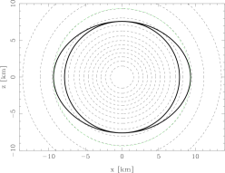
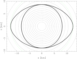
Figure 1: Two-fluid configurations with $\Omega_{\mathrm{n}}=2000\,\pi~{}\mathrm{s}^{-1}$ and $\Omega_{\mathrm{c}}=200\,\pi~{}\mathrm{s}^{-1}$. The thick lines represent the surfaces of the two fluids respectively, while the dashed lines are the isosurfaces of “gravitational potential” $\ln N$. In the left-hand configuration, the two fluids are locally non-interacting, i.e. $\kappa_{\mathrm{n}\mathrm{c}}=0$ and $\beta=0$, while in the right-hand configuration we have chosen $\kappa_{\mathrm{n}\mathrm{c}}=0.02$ and $\beta=0.12$.

Acknowledgements. RP acknowledges support from the EU Programme ’Improving the Human Research Potential and the Socio-Economic Knowledge Base’ (Research Training Network Contract HPRN-CT-2000-00137). GLC acknowledges partial support from NSF grant PHYS-0140138.

References

• [1] M. Baldo, J. Cugnon, A. Lejeune, and U. Lombardo. Nucl. Phys. A 536, 349 (1992).
• [2] O. Sjöberg. Nucl. Phys. A 265, 511 (1976).
• [3] B. Link and R.I. Epstein. ApJ 457, 844 (1996).
• [4] R. Prix. A&A 352, 623 (1999).
• [5] R. Prix, G.L. Comer, and N. Andersson. A&A 381, 178 (2002).
• [6] N. Andersson and G.L. Comer. Class. Quant. Grav.  18, 969 (2001).
• [7] B. Carter and D. Langlois. Nucl. Phys. B 531, 478 (1998).
• [8] D. Langlois, D.M. Sedrakian, and B. Carter. MNRAS 297, 1189 (1998).
• [9] B. Carter. In Relativistic Fluid Dynamics (Noto, 1987), eds. A. Anile and M. Choquet-Bruhat, (Springer, Heidelberg, 1989), pp. 1–64.
• [10] A.F. Andreev and E.P. Bashkin. JETP 42, 164 (1975).
• [11] S. Bonazzola, E. Gourgoulhon, M. Salgado, and J.A. Marck. A&A 278, 421 (1993).
• [12] S. Bonazzola, E. Gourgoulhon and J.A. Marck. Phys. Rev. D 58, 104020 (1998).