Gravitational Radiation from the radial infall of highly relativistic point particles into Kerr black holes

Abstract

In this paper, we consider the gravitational radiation generated by the collision of highly relativistic particles with rotating Kerr black holes. We use the Sasaki-Nakamura formalism to compute the waveform, energy spectra and total energy radiated during this process. We show that the gravitational spectrum for high-energy collisions has definite characteristic universal features, which are independent of the spin of the colliding objects. We also discuss possible connections between these results and the black hole-black hole collision at the speed of light process. With these results at hand, we predict that during the high speed collision of a non-rotating hole with a rotating one, about $35\%$ of the total energy can get converted into gravitational waves. Thus, if one is able to produce black holes at the Large Hadron Collider, as much as $35\%$ of the partons’ energy should be emitted during the so called balding phase. This energy will be missing, since we don’t have gravitational wave detectors able to measure such amplitudes. The collision at the speed of light between one rotating black hole and a non-rotating one or two rotating black holes turns out to be the most efficient gravitational wave generator in the Universe.

I Introduction

In previous works we have studied the collision at the speed of light between a point particle and a Schwarzschild black hole vitorjose1 , and a point particle and a Kerr black hole along its symmetry axis vitorjose2 . This analyses can describe several phenomena, such as, the collision between small and massive black holes schutz , the collision between stars and massive black holes, or the collision between highly relativistic particles like cosmic and gamma rays colliding with black holes piran , to name a few. We have argued in vitorjose1 ; vitorjose2 that these studies could give valuable quantitative answers for the collision at the speed of light between equal mass black holes, although we only work with perturbation theory à la Regge-Wheeler-Zerilli-Teukolsky-Sasaki-Nakamura, which formally does not describe this process. In fact, extrapolating for two equal mass, Schwarzschild black holes we obtained vitorjose1 results which were in very good agreement with results payne obtained through different methods. For equal mass black holes, we found that the collision at the speed of light between a Schwarzschild black hole and a Kerr black hole along the symmetry axis gave similar results to those in vitorjose1 . In particular, we found that $15.5\%$ of the total energy gets converted into gravitational waves (for two non-rotating holes the amount is slightly less, $13\%$). There are as yet no numerical results for rotating black holes, so there is no clue as to the correctness of our results for rotating holes. However, should these results give radiated energies larger than that allowed by the cosmic censorship, and therefore by the area theorem, we would run into problems, and we would know that the extrapolation to equal masses is strictly forbidden. Our previous results do not violate the area theorem, but the mere possibility brings us to the study of the collision of a non-rotating black hole with a rotating one, along the equatorial plane, both approaching each other at nearly the speed of light. Sasaki, Nakamura and co-workers nmothers have studied the infall of particles, at rest at infinity into Kerr black holes, along the equatorial plane and along the axis. They found that the energy radiated for radial infall along the equatorial plane was about $2.6$ times larger than for radial along the axis, for extreme holes. Accordingly, we expect the energy for highly relativistic collisions along the equatorial plane to be larger than that along the symmetry axis, but how larger? If the ratio $\frac{\Delta E_{{\rm equator}}}{\Delta E_{{\rm axis}}}$ should still be the same, $2.6$, then the energy released in the collision along the equatorial plane of a Kerr hole and a non-rotating hole at the speed of light would be $\sim 40\%$ of the total energy. But this is slightly more than the upper bound on the efficiency allowed by the area theorem, which is $\sim 38.7\%$. Motivated mainly by this scenario, we shall study here the collision at nearly the speed of light between a point particle and a Kerr black hole, along its equatorial plane. We will then perform a boost in the Kerr black hole, and extrapolate for two equal mass objects, one rotating, the other non-rotating.

Another point of interest to study this process is the hypothesis that black holes could be produced at the Large Hadron Collider (LHC) at CERN, which has recently been put forward bhprod in the so called TeV-scale gravity scenarios. In such scenarios, the hierarchy problem is solved by postulating the existence of $n$ extra dimensions, sub-millimeter sized, such that the $4+n$ Planck scale is equal to the weak scale $\sim$ 1TeV. The Standard Model lives on a 4-dimensional sub-manifold, the brane, whereas gravity propagates in all dimensions. If TeV-scale gravity is correct, then one could manufacture black holes at the LHC. The ability to produce black holes would change the status of black hole collisions from a rare event into a human controlled one. This calls for accurate predictions of gravitational wave spectra and gravitational energy emitted during black hole formation from the high speed encounter of two particles. This investigation was first carried out by D’Eath and Payne payne by doing a perturbation expansion around the Aichelburg-Sexl metric, describing a boosted Schwarzschild black hole. Their computation was only valid for non-rotating black holes and it seems quite difficult to extend their methods to include for spinning black holes. Our approach however allows one to also study spinning black holes, which is of great importance, since if one forms black holes at the LHC, they will most probably be rotating ones, the chance for having a zero impact parameter being vanishingly small.

Suppose therefore one can produce black holes at LHC. The first thing that should happen is a release of the hole’s hair, in a phase termed “balding” bhprod . The total amount of energy released in such a phase is not well known, and is based mostly in D’Eath and Payne’s results. With our results one can predict the total gravitational energy radiated in the balding phase when the resulting holes are rotating, a process which, as we shall see, radiates a tremendous amount of energy. This means that there will be a “missing” energy during the formation of a black hole, this energy being carried away by gravitational waves, and undetected, at least by any realistic present technology. Our results suggest that as much as 35% of the center of mass energy can be leaking away as gravitational waves, and therefore one should have 35% missing energy. Strictly speaking, these values are only valid for a head-on collision, i.e. a collision with zero impact parameter, along the equatorial plane. One expects the total energy to decrease if the collision is taken along a different plane, or with non-zero impact parameter. However, we do not expect the total energy to vary much as long as the impact parameter stays sufficiently small enough to give rise to black hole production.

II The Teukolsky and Sasaki-Nakamura formalism

In this section, we give a very brief account of the Teukolsky equation, and of the Sasaki-Nakamura equation. Details about the Teukolsky formalism may be found in the original literature teukolsky , and also in breuerbook . For a good account of the Sasaki-Nakamura formalism we refer the reader to nmothers ; nakamurasasaki ; hughes1 .

We start from the Kerr background geometry, written in Boyer-Lindquist $(t,r,\theta,\phi)$ coordinates:

$$ds^{2}=-(1-\frac{2Mr}{\Sigma})dt^{2}-\frac{4Mar}{\Sigma}\sin^{2}\theta dtd\phi+\frac{\Sigma}{\Delta}dr^{2}+\Sigma d\theta^{2}+\frac{A\sin^{2}\theta}{\Sigma}d\phi^{2}\,,$$ (1)

Here, $M$ is the mass of the black hole, and $a$ its angular momentum per unit mass. Also $\Sigma=r^{2}+a^{2}\cos^{2}\theta\,$ ; $\Delta=r^{2}+a^{2}-2Mr\,$ ; $A=(r^{2}+a^{2})^{2}-\Delta a^{2}\sin^{2}\theta$.

Working with Kinnersley’s null tetrad, one can show teukolsky that the equations for the Newman-Penrose quantities decouple and separate, giving rise to the Teukolsky equation,

$$\Delta^{-s}\frac{d}{dr}(\Delta^{s+1}\frac{d}{dr}{{}_{s}R})-\,_{s}V\,_{s}R=-\,_{s}T\,.$$ (2)

Here,

$${}_{s}V=\frac{-K^{2}}{\Delta}+\frac{isK\Delta^{\prime}}{\Delta}-\frac{2isK^{\prime}}{\Delta}-2isK^{\prime}+\,_{s}\lambda$$ (3)

$$K=(r^{2}+a^{2})\omega-am\,,$$ (4)

and a prime denotes derivative with respect to $r$. The quantity $s$ denotes the spin weight (or helicity) of the field under consideration (see for example newman ) and $m$ is an azimuthal quantum number. We are interested in gravitational perturbations, which have spin-weight $s=-2,+2$. Solutions with $s=-2$ are related to those with $s=2$ via the Teukolsky-Starobinsky identities, so we need only worry about a specific one. For definiteness, and because that was the choice adopted by Sasaki and others nmothers , we work with $s=-2$. The constants $m$, ${}_{s}\lambda$ (${}_{s}\lambda$ depends non-linearly on $\omega$) are separation constants arising from the azimuthal function $e^{im\phi}$ and the angular eigenfunction $\,{}_{s}Z_{lm}^{a\omega}(\theta,\phi)$, respectively. $\,{}_{s}Z_{lm}^{a\omega}(\theta,\phi)$ is the spin-weighted spheroidal harmonic, ${}_{s}Z_{lm}^{a\omega}(\theta,\phi)=\frac{1}{(2\pi)^{1/2}}\,_{s}S_{lm}^{a\omega}(\theta)e^{im\phi}$, and in turn, ${}_{s}S_{lm}^{a\omega}(\theta)$ satisfies

$$\frac{1}{\sin\theta}\frac{d}{d\theta}(\sin\theta\frac{d}{d\theta}{S})+(a^{2}\cos^{2}\theta-\frac{m^{2}}{\sin^{2}\theta}+4a\omega\cos\theta+\frac{4m\cos\theta}{\sin^{2}\theta}-4\cot^{2}\theta+c)S=0\,,$$ (5)

where $c=\lambda-2-a^{2}\omega^{2}+2am\omega$. The spheroidal functions are normalized according to $\int d\Omega|_{s}Z_{lm}^{a\omega}(\theta,\phi)|^{2}=1$. These functions have not been thoroughly exploited as far as we know, but the essentials, together with tables for the eigenvalues $\lambda$ for $s=-2$ can be found in pressteu ; breuer . The source term ${}_{s}T$ appearing in (2) may be found in breuerbook , and depends on the stress-energy tensor of the perturbation under consideration. We note that, for a test particle falling in from infinity with zero velocity, for example, $T\sim r^{7/2}$ and $V$ is always long-range. This means that when we try to solve the Teukolsky equation (2) numerically we will run into problems, since usually the numerical solution is accomplished by integrating the source term times certain homogeneous solutions. At infinity this integral will not be well defined since the source term explodes there, and also because since the potential is long range, the homogeneous solution will also explode at infinity. We can remedy this long-range nature of the potential and at the same time regularize the source term in the Sasaki-Nakamura formalism. After a set of transformations, the Teukolsky equation (2) may be brought to the Sasaki-Nakamura form nakamurasasaki :

$$\frac{d^{2}}{dr_{*}^{2}}{X(\omega,r)}-{\cal F}\frac{d}{dr_{*}}{X(\omega,r)}-{\cal U}X(\omega,r)={\cal L}\,.$$ (6)

The functions ${\cal F}$ and ${\cal U}$ can be found in the original literature nmothers ; nakamurasasaki . The source term ${\cal L}$ is given by

$${\cal L}=\frac{\gamma_{0}\Delta}{r^{2}(r^{2}+a^{2})^{3/2}}We^{-i\int K/\Delta dr_{*}}\,,$$ (7)

and $W$ satisfies

$$W^{\prime\prime}=-\frac{r^{2}}{\Delta}Te^{i\int K/\Delta dr_{*}}.$$ (8)

The tortoise $r_{*}$ coordinate is defined by $dr_{*}/dr=(r^{2}+a^{2})/\Delta$, and ranges from $-\infty$ at the horizon to $+\infty$ at spatial infinity. The Sasaki-Nakamura equation (6) is to be solved under the “only outgoing radiation at infinity” boundary condition (see section 4.2), meaning

$$X(\omega,r)=X^{{\rm out}}e^{i\omega r_{*}}\,,r_{*}\rightarrow\infty.$$ (9)

The two independent polarization modes of the metric, $h_{+}$ and $h_{\times}$, are given by

$$h_{+}+ih_{\times}=\frac{8}{r\sqrt{2\pi}}\int_{-\infty}^{+\infty}d\omega\sum_{l,m}e^{i\omega(r_{*}-t)}\frac{X^{{\rm out}}S_{lm}^{a\omega}(\theta)}{\lambda(\lambda+2)-12i\omega-12a^{2}\omega^{2}}e^{im\phi},$$ (10)

and the power per frequency per unit solid angle is

$$\frac{d^{2}E}{d\Omega d\omega}=\frac{4\omega^{2}}{\pi}|\sum_{l,m}\frac{X^{{\rm out}}}{\lambda(\lambda+2)-12i\omega-12a^{2}\omega^{2}}S_{lm}^{a\omega}|^{2}.$$ (11)

Following Nakamura and Sasaki nmothers the multipolar structure is given by

$$h_{+}+ih_{\times}=-\frac{(2\pi)^{1/2}}{r}\int_{-\infty}^{+\infty}d\omega\sum_{l,m}e^{i\omega(r_{*}-t)}\left[h^{lm}(\omega)_{-2}Y_{lm}\right]e^{im\phi},$$ (12)

which defines $h^{lm}$ implicitly. Moreover,

$$\Delta E=\frac{\pi}{4}\int_{0}^{\infty}\sum_{lm}|h^{lm}(\omega)|^{2}+|h^{lm}(-\omega)|^{2}.$$ (13)

Here, ${}_{-2}Y_{lm}(\theta)$ are spin-weighted spherical harmonics (basically ${}_{2}S_{lm}^{a\omega=0}(\theta)$), whose properties are described by Newman and Penrose newman and Goldberg et al goldberg .

For the befenit of comparison, the general relation between Sasaki and Nakamura’s $X(\omega,r)$ function and Teukolsky’s $R(\omega,r)$ function is given in nmothers is terms of some complicated expressions. One finds however that near infinity, which is the region we are interested in, this relation simplifies enormously. In fact, when $r_{*}\rightarrow\infty$, the relation is

$$R=R^{{\rm out}}r^{3}e^{i\omega r_{*}}\,$$ (14)

where,

$$R^{{\rm out}}\equiv-\frac{4\omega^{2}X^{{\rm out}}}{\lambda(\lambda+2)-12i\omega-12a^{2}\omega^{2}}\,.$$ (15)

III The Sasaki-Nakamura equations for a point particle falling along a geodesic of the Kerr black hole spacetime

The dependence of the emitted gravitational wave power on the trajectory of the particle comes entirely from the source ${\cal L}$ in eqs. (6)-(7), which in turn through (8) depends on the source term $T$ in Teukolsky’s equation (2). To compute the explicit dependence, one would have to consider the general expression for the geodesics in the Kerr geometry chandra , which in general gives an end result not very amenable to work with. However we find that by working in the highly relativistic regime, the equations simplify enormously, and in particular for radial infall (along the symmetry axis or along the equator) it is possible to find a closed analytic and simple expression for $W$ in (7)-(8). Accordingly, we shall in the following give the closed expressions for ${\cal L}$ in these two special situations: radiall infall along the symmetry axis and radial infall along the equator of an highly energetic particle.

III.1 The Sasaki-Nakamura equations for an highly relativistic point particle falling along the symmetry axis of the Kerr black hole

We now specialize then all the previous equations to the case under study. We suppose the particle to be falling radially along the symmetry axis of the Kerr hole, in which case all the equations simplify enormously. In this case the geodesics, written in Boyer-Lindquist coordinates, are

$$\frac{dt}{d\tau}=\frac{\epsilon_{0}(r^{2}+a^{2})}{\Delta}\,;\quad\,(\frac{dr}{d\tau})^{2}=\epsilon_{0}^{2}-\frac{\Delta}{r^{2}+a^{2}}\,;\quad\frac{d\phi}{d\tau}=\frac{a\epsilon_{0}}{\Delta}\,,$$ (16)

where the parameter $\epsilon_{0}$ is the energy per unit rest mass of the infalling particle. On considering highly relativistic particles, $\epsilon_{0}\rightarrow\infty$, we find that the term ${\cal L}$ takes the simple form (compare with the source term in vitorjose1 ; vitorjose2 ) :

$${\cal L}=-\frac{\mu C\epsilon_{0}\gamma_{0}\Delta}{2\omega^{2}r^{2}(r^{2}+a^{2})^{3/2}}e^{-i\omega r_{*}}.$$ (17)

Here, $C=\left[\frac{8Z_{l0}^{a\omega}}{\sin^{2}\theta}\right]_{\theta=0}$, the function $\gamma_{0}=\gamma_{0}(r)$ can be found in nmothers , while $\mu$ is the mass of the particle.

III.2 The Sasaki-Nakamura equations for an highly relativistic point particle falling along the equatorial plane of the Kerr black hole

We now suppose the particle is falling radially along the equator of the Kerr hole, where radially is defined in the sense of Chandrasekhar chandra , meaning that $L=a\epsilon_{0}$, where $L$ is the conserved angular momentum. In this case the geodesics, written in Boyer-Lindquist coordinates, are

$$\frac{dt}{d\tau}=\frac{\epsilon_{0}(r^{2}+a^{2})}{\Delta}\,;\quad\,r^{2}(\frac{dr}{d\tau})^{2}=\epsilon_{0}^{2}r^{2}-\Delta\,;\quad\frac{d\phi}{d\tau}=\frac{a\epsilon_{0}}{\Delta}\,.$$ (18)

On considering highly relativistic particles, $\epsilon_{0}\rightarrow\infty$, we find that the source term takes again a very simple form (compare with the source term in vitorjose1 ; vitorjose2 ):

$${\cal L}=-\frac{\mu\hat{S}\epsilon_{0}\gamma_{0}\Delta}{\omega^{2}r^{2}(r^{2}+a^{2})^{3/2}}e^{-i\int\frac{K}{\Delta}dr}\,,$$ (19)

where

$$\hat{S}=\left[\frac{\lambda}{2}-(m-a\omega)^{2}\right]Z_{lm}({\theta=\frac{\pi}{2}})+\left[(m-a\omega)\right]Z^{\prime}_{lm}({\theta=\frac{\pi}{2}})$$ (20)

Once $X^{{\rm out}}$ is known, we can get the Teukolsky wavefunction near infinity from (14), and the waveform and energy spectra from (10)-(13).

IV Implementing a numerical solution

To compute the spin-weighted spheroidal functions, one would have to compute the eigenvalues $\lambda$, for each $\omega$, using a shooting method numrecipes or any other numerical scheme one chooses nmothers ; hughes1 . We have chosen to lean ourselves on work already done by Press and Teukolsky pressteu and to verify at each step the correctness of their results (we found no discrepancies). Press and Teukolsky have found, for each ($l$, $m$), a sixth-order polynomial (in $a\omega$) which approximates the eigenvalue $\lambda$, to whithin five decimal places (see their Table 1). This is a good approximation as long as $a\omega<3$, which is within our demands for $l<6$. The computation of the spheroidal function then follows trivially, by numerically integrating (5).

The next step is to determine $X(\omega,r)$ from the Sasaki-Nakamura differential equation (6). This is accomplished by a Green’s function technique, constructed so as to satisfy the usual boundary conditions, i.e., only ingoing waves at the horizon ($X\sim e^{-i\omega r_{*}}\,,r_{*}\rightarrow-\infty$) and outgoing waves at infinity($X\sim e^{i\omega r_{*}}\,,r_{*}\rightarrow\infty$). We get that, near infinity, and for infall along the equator (we are interested in knowing the wavefunction in this region),

$$X=X^{\infty}\int\frac{X^{H}{\cal S}}{{\rm Wr}}dr_{*}\,;\quad X^{\rm out}=\int\frac{X^{H}{\cal S}}{{\rm Wr}}dr_{*}.$$ (21)

The similar expression for infall along the symmetry axis is given in vitorjose2 . Here, $X^{\infty}$ and $X^{H}$ are two linearly independent homogeneous solutions of (6) which asymptotically behave as

$$X^{H}\sim A(\omega)e^{i\omega r_{*}}+B(\omega)e^{-i\omega r_{*}}\,,r_{*}\rightarrow\infty$$ (22)

$$X^{H}\sim e^{-i\omega r_{*}}\,,r_{*}\rightarrow-\infty$$ (23)

$$X^{\infty}\sim e^{i\omega r_{*}}\,,r_{*}\rightarrow\infty$$ (24)

$$X^{\infty}\sim C(\omega)e^{i\omega r_{*}}+D(\omega)e^{-i\omega r_{*}}\,,r_{*}\rightarrow-\infty\,,$$ (25)

and ${\rm Wr}$ is the wronskian of these two solutions. Expression (21) can be further simplified in the case of infall along the equator to

$$X^{{\rm out}}=-\frac{\mu\epsilon_{0}c_{0}\hat{S}}{2i\omega^{3}B}\int\frac{e^{-i\int\frac{K}{\Delta}dr}X^{H}}{r^{2}(r^{2}+a^{2})^{1/2}}dr.$$ (26)

To implement a numerical solution, we first have to determine $B(\omega)$. We find $B(\omega)$ by solving (6) with the right hand side set to zero, and with the starting condition $X^{H}=e^{-i\omega r_{*}}$ imposed at a large negative value of $r_{*}$. For computational purposes good accuracy is hard to achieve with the form (22), so we used an asymptotic solution one order higher in $1/(\omega r)$:

$$X^{H}=A(\omega)(1+\frac{i(\lambda+2+2am\omega-2i\omega P)}{2\omega r})e^{i\omega r_{*}}+$$

$$+B(\omega)(1-\frac{i(\lambda+2+2am\omega-2i\omega P)}{2\omega r})e^{-i\omega r_{*}}\,,r_{*}\rightarrow+\infty\,.$$ (27)

Here, $P=\frac{8ai(-m\lambda+a\omega(\lambda-3))}{12a^{2}\omega^{2}+12iM\omega-\lambda^{2}-2\lambda-12am\omega}$. These expressions all refer to the case of infall along the equator. For analogous expressions for infall along the symmetry axis see vitorjose2 .

In the numerical work, we chose to adopt $r$ as the independent variable, thereby avoiding the numerical inversion of $r_{*}(r)$. A fourth order Runge-Kutta routine started the integration of $X^{H}$ near the horizon, at $r=r_{+}+r_{+}\epsilon$ (the horizon radius $r_{+}$ is $r_{+}=M+(M^{2}-a^{2})^{1/2}$), with tipically $\epsilon=10^{-5}$. It then integrated out to large values of $r$, where one matches $X^{H}$ extracted numerically with the asymptotic solution (27), in order to find $B(\omega)$. To find $\Delta E$ the integral in (13) is done by Simpson’s rule. For both routines Richardson extrapolation is used.

V Numerical Results and Conclusions

Recent studies vitorjose1 ; vitorjose2 on high energy collisions of point particles with black holes point to the existence of some characteristic features of these processes, namely: (i) the spectrum and waveform largely depend upon the lowest quasinormal frequency of the spacetime under consideration; (ii) there is a non-vanishing zero frequency limit (ZFL) for the spectra, $\frac{dE}{d\omega}_{\omega\rightarrow 0}$, and it seems to be independent of the spin of the colliding particles whereas for low-energy collisions the ZFL is zero; (iii) the energy radiated in each multipole has a power-law dependence rather than exponential for low-energy collisions.

The present study reinforces all these aspects. In Fig. 1 we show, for an almost extreme Kerr hole with $a=0.999M$, the energy spectra for the four lowest values of $l$, when the particle collides along the equatorial plane. In Fig. 2 we show the same values but for a collision along the symmetry axis. The existence of a non-vanishing ZFL is evident, but the most important in this regard is that the ZFL is exactly the same, whether the black hole is spinning or not, or whether the particle is falling along the equator or along the symmetry axis. In fact, our numerical results show that, up to the numerical error of about $1\%$ the ZFL is given by Table 1 (see also vitorjose1 and the exact value given by Smarr smarr2 ), and this holds for highly relativistic particles falling along the equator (present work), along the symmetry axis vitorjose2 , or falling into a Schwarzschild black hole vitorjose1 .

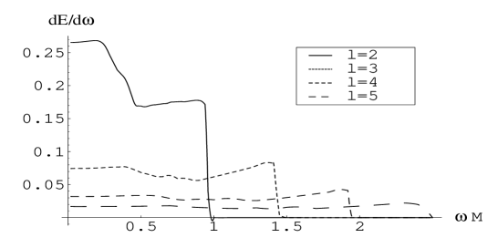
Figure 1: The energy spectra for a point particle moving at nearly the speed of light and colliding, along the equatorial plane, with an extreme (a=0.999M) Kerr black hole. The energy is normalized in units of $\mu^{2}\epsilon_{0}^{2}$. Notice that the spectra is almost flat (for large $l$), the ZFL is non-vanishing and that the quadrupole carries less than half of the total radiated energy.

Figure 2: The energy spectra for a point particle moving at nearly the speed of light and colliding, along the symmetry axis, with an extreme (a=0.999M) Kerr black hole. The energy is normalized in units of $\mu^{2}\epsilon_{0}^{2}$. Notice that the spectra is almost flat (for large $l$), the ZFL is non-vanishing and that the quadrupole carries less than half of the total radiated energy.

Table 1: The zero frequency limit (ZFL) for the ten lowest radiatable multipoles.

$l$	ZFL($\times\frac{1}{\mu^{2}\epsilon_{0}^{2}}$)	$l$	ZFL($\times\frac{1}{\mu^{2}\epsilon_{0}^{2}}$)
2	0.265	7	0.0068
3	0.075	8	0.0043
4	0.032	9	0.003
5	0.0166	10	0.0023
6	0.01	11	0.0017

The $l$-dependence of the energy radiated is a power-law; in fact for large $l$ we find for infall along the equator

$$\Delta E_{l}=0.61\frac{\mu^{2}\epsilon_{0}^{2}}{Ml^{1.666}}\;\;,\quad\quad a=0.999M.$$ (28)

Such a power-law dependence seems to be universal for high energy collisions. Together with the universality of the ZFL this is one of the most important results borne out of our numerical studies. The exponent of $l$ in (28) depends on the rotation parameter. As $a$ decreases, the exponent increases monotonically, until it reaches the Schwarzschild value of 2 ($\Delta E_{l}\sim\frac{1}{l^{2}}$) which was also found for particles falling along the symmetry axis of a Kerr hole. In Table 2 we show the values of the exponent, as well as the total energy radiated, for some values of the rotation parameter $a$.

$\Delta E_{l}=cl^{-b}$
$\frac{a}{M}$	$c$	$b$	$\Delta E_{{\rm tot}}\frac{M}{\mu^{2}\epsilon_{0}^{2}}$
0.999	0.61	1.666	0.69
0.8	0.446	1.856	0.36
0.5	0.375	1.88	0.29
0	0.4	2	0.26

Table 2. Power-law dependence of the energy radiated in each multipole $l$, here shown for some values of $a$, the rotation parameter. We write $\Delta E_{l}=\frac{c}{l^{b}}$ for the energy emitted for each $l$ and $\Delta E_{{\rm tot}}$ for the total energy radiated away. The collision happens along the equatorial plane.

This power-law dependence and our numerical results allow us to infer that the total energy radiated for a collision along the equator is

$$\Delta E_{{\rm tot}}=0.69\frac{\mu^{2}\epsilon_{0}^{2}}{M}\;\;,\quad\quad a=0.999M.$$ (29)

This represents a considerable enhancement of the total radiated energy, in relation to the Schwarzschild case vitorjose1 or even to the infall along the symmetry axis vitorjose2 . Again, the energy carried by the $l=2$ mode ($\Delta E_{l=2}=0.2\frac{\mu^{2}\epsilon_{0}^{2}}{M}\;,\;\;a=0.999M$) is much less than the total radiated energy.

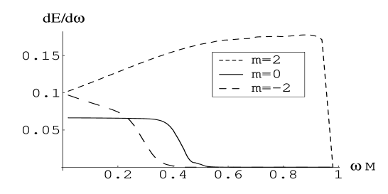
Figure 3: The energy spectra as a function of $m$ for $l=2$ and for an highly relativistic particle falling along the equatorial plane of a Kerr black hole. The energy is normalized in units of $\mu^{2}\epsilon_{0}^{2}$.

Figure 4: The $l=2$ waveform as defined by (12) for an highly relativistic particle falling along the equatorial plane of an extreme (a=0.999) Kerr black hole.The waveform is normalized in units of $\mu\epsilon_{0}$.

In Fig. 3 we show, for $l=2$, the energy spectra as a function of $m$, which allows us to see clearly the influence of the quasinormal modes. Indeed, one can see that the energy radiated for $m=2$ is much higher than for $m=-2$, and this is due to the behaviour of the quasinormal frequency for different azimuthal numbers $m$ QNKerr , as emphasized by different authors nmothers . A peculiar aspect is that the energy radiated for $m+l=$ odd is about two orders of magnitude lower than for $m+l=$ even, and that is why the spectra for $m=-1,1$ is not plotted in Fig. 3. Notice that the ZFL is the same for $m=2$ and for $m=-2$ both conspiring to make the ZFL universal. In Fig. 4 we show the $l=2$ waveform for $a=0.999M$ as seen in $\phi=0\,,\theta=\pi/2$. By symmetry, $h_{\times}=0$.

Up to now, we dealt only with the head-on collision between a particle and a black hole. What can we say about collisions with non-zero impact parameter, and along the equator ? As is clear from our results, the fact that the quasinormal modes are excited is fundamental in obtaining those high values for the total energy radiated. Previous studies QNKerr show that the quasinormal modes are still strongly excited if the impact parameter is less than $2M$. We are therefore tempted to speculate that as long as the impact parameter is less than $2M$ the total energy radiated is still given by Table 2. For larger values of the impact parameter, one expects that total energy to decrease rapidly. On the other hand, If the collision is not along the equatorial plane, we do expect the total energy to decrease. For example, if the collision is along the symmetry axis, we know vitorjose2 that the total energy is $0.31\frac{\mu^{2}\epsilon_{0}^{2}}{M}$ for $a=0.999M$. So we expect that as the angle between the collision axis and the equator is varied between $0$ and $\pi/2$ the total energy will be a monotonic function decreasing from $0.69\frac{\mu^{2}\epsilon_{0}^{2}}{M}$ to $0.31\frac{\mu^{2}\epsilon_{0}^{2}}{M}$. Still, more work is necessary to confirm this. Let us now consider, using these results, the collision at nearly the speed of light between a Schwarzschild and a Kerr black hole, along the equatorial plane. We have argued in previous papers vitorjose1 ; vitorjose2 that the naive extrapolation $\mu\rightarrow M$ may give sensible results, so let’s pursue that idea here. We obtain an efficiency of $34.5\%$ for gravitational wave generation, a remarkable increase relative to the Schwarzschild-Schwarzschild collision. Now, the area theorem gives an upper limit of $38.7\%$ so we may conclude with two remarks: (a) these perturbative methods pass the area theorem test; (b) we are facing the most energetic events in the Universe, with the amazing fraction of $34.5\%$ of the rest mass being converted into gravitational waves.

References

- (1) V. Cardoso and J. P. S. Lemos, Phys. Lett. B B 538, 1 (2002).
- (2) V. Cardoso and J. P. S. Lemos, Gen. Rel. Gravitation (in press), gr-qc/0207009.
- (3) B. F. Schutz, Class. Q uant. Grav. 16, A131 (1999).
- (4) T. Piran, Gravitational Waves: A Challenge to Theoretical Astrophysics, edited by V. Ferrari, J.C. Miller and L. Rezzolla (ICTP, Lecture Notes Series).
- (5) P. D. D’Eath and P. N. Payne, Phys. Rev. D 46, 658 (1992); Phys. Rev. D 46, 675 (1992); Phys. Rev. D 46, 694 (1992).
- (6) M. Sasaki and T. Nakamura, Prog. Theor. Phys. 67, 1788 (1982); T. Nakamura and M. Sasaki, Phys. Lett. 89A, 185 (1982); Y. Kojima and T. Nakamura, Phys. Lett. 96A, 335 (1983); Y. Kojima and T. Nakamura, Phys. Lett. 99A, 37 (1983); Y. Kojima and T. Nakamura, Prog. Theor. Phys. 71, 79 (1984).
- (7) G. Landsberg, hep-ph/0211043; M. Cavaglia, hep-ph/0210296; D. M. Eardley and S. B. Giddings, Phys. Rev. D66, 044011 (2002); H. Yoshino and Y. Nambu, gr-qc/0209003; P. Kanti and J. March-Russell, Phys. Rev. D66, 024023 (2002). P. Kanti and J. March-Russell, hep-ph/0212199. D. Ida, Kin-ya Oda and S. C. Park, hep-th/0212108.
- (8) S. A. Teukolsky, Astrophys. J. 185, 635 (1973).
- (9) R. A. Breuer, in Gravitational Perturbation Theory and Synchrotron Radiation, (Lecture Notes in Physics, Vol. 44), (Springer, Berlin 1975).
- (10) T. Nakamura and M. Sasaki, Phys. Lett. 89A, 68 (1982); M. Sasaki and T. Nakamura, Phys. Lett. 87A, 85 (1981).
- (11) S. A. Hughes, Phys. Rev. D 61, 0804004 (2000); D. Kennefick, Phys. Rev. D 58, 064012 (1998);
- (12) E. Newman and R. Penrose, J. Math. Phys. 3, 566 (1966);
- (13) W. H. Press and S. A. Teukolsky, Astrophys. J. 185, 649 (1973).
- (14) R. A. Breuer, M. P. Ryan Jr, and S. Waller, Proc. R. Soc. London A358, 71 (1977).
- (15) J. N. Goldberg, A. J. MacFarlane, E. T. Newman, F. Rohrlich and C. G. Sudarshan, J. Math. Phys. 8, 2155 (1967);
- (16) S. Chandrasekhar, in The Mathematical Theory of Black Holes, (Oxford University Press, New York, 1983).
- (17) W. H. Press, B. P. Flannery, S. A. Teukolsky and W. T. Vetterling, Numerical Recipes (Cambridge University Press, Cambridge, England, 1986).
- (18) L. Smarr, Phys. Rev. D 15, 2069 (1977).
- (19) S. Detweiler, Astrophys. J. 239, 292 (1980); V. Ferrari and B. Mashhoon, Phys. Rev. D 30, 295 (1984); V. Ferrari and B. Mashhoon, Phys. Rev. Lett. 52, 1361 (1984); V. P. Frolov, and I. D. Novikov, in Black Hole Physics - Basic Concepts and New Developments, (Kluwer Academic Publishers, Dordrecht, 1998).