Searching for Gravitational Waves from the Inspiral of Precessing Binary Systems: New Hierarchical Scheme using “Spiky” Templates

Abstract

In a recent investigation GrandKV02 of the effects of precession on the anticipated detection of gravitational-wave inspiral signals from compact object binaries with moderate total masses $\lesssim 10\,M_{\odot}$, we found that (i) if precession is ignored, the inspiral detection rate can decrease by almost a factor of $10$, and (ii) previously proposed Apost96 “mimic” templates cannot improve the detection rate significantly (by more than a factor of 2). In this paper we propose a new family of templates that can improve the detection rate by factors of 5–6 in cases where precession is most important. Our proposed method for these new “mimic” templates involves a hierarchical scheme of efficient, two-parameter template searches that can account for a sequence of spikes that appear in the residual inspiral phase, after one corrects for the any oscillatory modification in the phase. We present our results for two cases of compact object masses ($10$ and $1.4$ M_⊙ and $7$ and $3$ M_⊙) as a function of spin properties. Although further work is needed to fully assess the computational efficiency of this newly proposed template family, we conclude that these “spiky templates” are good candidates for a family of precession templates used in realistic searches, that can improve detection rates of inspiral events.

I Introduction

The inspiral of binary compact objects is one of the main targets of the ground-based, interferometric gravitational-wave detectors currently coming online (LIGO Abram92 , VIRGO Caron97 , GEO600 Danzm95 and TAMA Tagos01 ). It is well known that the most effective way of extracting such signals from the intrinsic noise of the detectors is to use matched-filtering techniques Helst68 ; OwenS99 ; Finn99 , which involves the correlation of detector output with a family of templates thought to represent the expected signals. It is clear that the success of such searches critically depends on the accuracy of the adopted template families.

A great effort has been devoted to the computation of compact object inspiral waveforms, especially using various PN-expansions (see CutleT02 for a review). The current searches in LIGO, GEO600 and TAMA, are performed using the template family corresponding to two, non-spinning, point masses, including 2.5-PN order corrections. However, in some cases, expected signals are believed to deviate significantly from these waveforms. For the case of massive compact binaries (total mass in excess of $10$ M_⊙), it has been shown that the PN approximations break down right in the frequency band of the interferometric detectors BradyCT98 . In fact the exact signal is unknown and a number of different approximations have been suggested as alternatives. Recently, a family of templates that exhibits good overlap with the results obtained using all the various expansion approximations has been suggested for use in future searches (see BuonaCV02 and references therein).

Another case where the current template family does not reflect realistic signals is the case of precessing binaries. Compact objects with spins of significant magnitude and misalignment relative to the orbital angular momentum axis emit inspiral signals that are mainly modified by precession of the orbital plane ApostCST94 . This precession is caused by high-order spin-orbit and spin-spin couplings. Depending on the physical properties of the binary, a significant number of precession cycles occur within the frequency band of current ground-based interferometers. The resulting change in the polarization of the wave leads to modulations of both the amplitude and the phase of the inspiral signal. In principle, one would like to build a family of precessing inspiral templates. However, this is unrealistic because of computational limitations: precessing waveforms depend on extra parameters (spin magnitudes and orientations) and make the dimension of template parameter space prohibitively large. The first investigations of the importance of precession ApostCST94 were further expanded in a consistent way GrandKV02 (hereafter Paper I) to account for the current LIGO noise curve and all possible physical configurations of intermediate-mass $\lesssim 10\,M_{\odot}$ systems. It is now understood that ignoring precession in the templates could risk the anticipated inspiral detection, since the detection rate can be reduced by almost an order of magnitude in the worst cases. The need for a family of “mimic” templates that can capture the signal modifications without unreasonably expanding the dimensionality of the templates is clear. Early on Apost96 suggested such a family that depends on only 3 additional parameters. In Paper I we tested it extensively and found that this family alone did not improve the detection rate significantly (improvement factors remained lower than 2 regardless of spin properties and masses).

Our motivation for this paper is to pursue the issue of “mimic” precession templates further. Throughout this work the methods and notations are the same as in Paper I. The precessing signals are obtained using the simple-precession formalism ApostCST94 ; Apost95 , where only the most massive object carries a spin (see the Introduction of Paper I for a justification). In this regime, the effect of precession is described by both a phase and an amplitude modulation, so that, in the frequency domain, the signal is given by

$$\tilde{h}_{\rm prec}\left(f\right)={\rm AM}\times{\rm PM}\times\tilde{h}_{\rm no\,prec}\left(f\right).$$ (1)

In Eq. (1), $\tilde{h}_{\rm no\,prec}$ denotes the signal with the same physical parameters (masses, orientations …) but without precession. ${\rm AM}$ is an amplitude modulation (Eq. (11) of Apost95 ) and ${\rm PM}=\exp\left(-i\phi_{\rm mod}\right)$ is a phase modulation (Eq. (12) of Apost95 ). We will neglect the Thomas precession (Eq. (14) of Apost95 ), assuming that the monotonic modulation induced by it will not greatly influence the results. This assumption should be checked by future work. Except when otherwise stated, the non-precessing parts of the templates and the signal, $\tilde{h}_{\rm no\,prec}$, are Newtonian. This is a simplifying assumption that makes our calculations feasible, given our current computational resources. We have already shown in Paper I that this assumption does not affect our results and conclusion in any quantitative way.

In this paper we have again included some indicative runs (of high computational cost) to show that the assumption of Newtonian non-precessing parts of the templates and the signal (as long as the two are consistent with each other; cf. Apost96 ) is not in any way limiting. We adopt a noise curve relevant to the initial LIGO. The efficiency of a family of templates is quantified by the concept of the fitting factor (FF) ApostCST94 , which describes the loss in signal-to-noise ratio (SNR) due to the mismatch between the signal and the templates:

$$\left(\frac{S}{N}\right)=\mathrm{FF}\times\left(\frac{S}{N}\right)_{\mathrm{max}}$$ (2)

where $\left(S/N\right)_{\mathrm{max}}$ is the SNR that would be achieved if the family of templates included the signal (see Apost96 ; Helst68 ; ApostCST94 ; Finn99 for more details). Most of the results will be presented by plotting the quantity $\mathrm{<FF>}^{3}$, the factor by which the detection rate is reduced, assuming a uniform distribution of sources in volume and using the fitting factor averaged over all random angles in the problem.

This paper is organized as follows. In Sec.II, we first provide a physical explanation for why the Apostolatos’ “mimic” template family is insufficient, in the context of an example case analyzed in detail. Motivated by the results in the first part, we introduce a new family of templates, and show how they can improve the SNR of detections. After briefly reviewing the determination of various computational parameters, we present our comprehensive results for two cases of high precession ($\left(m_{1},m_{2}\right)=\left(10,1.4\right)$ and $\left(m_{1},m_{2}\right)=\left(7,3\right)$ in M_⊙). Conclusions, perspectives, and future work are discussed in Sec. IV.

II New family of templates

II.1 Plausible explanation for the insufficiency of Apostolatos’ “mimic” templates

The Apostolatos’ “mimic” templates consist of non-precessing waveforms modulated in phase by the following oscillatory mathematical form:

$$\phi^{\rm cor}={\mathcal{C}}\cos\left({\mathcal{B}}f^{-2/3}+\delta\right)$$ (3)

In the simple precession regime Apost96 ; ApostCST94 ; Apost95 , both the spin $\vec{S}$ and the orbital momentum $\vec{L}$ precess around the total angular momentum $\vec{J}$, which remains at an approximately constant direction. Analytical, approximate formulae (Eqs. (29) of Apost95 ) of the precession angle (i.e. the angle describing the position of $\vec{L}$ along its precession cone), as a function of frequency, have been derived. It has been argued that the modulation of the inspiral phase induced by precession would have essentially the same behavior with respect to frequency, hence the form (3).

There was also an expectation that any monotonic modulation of the phase would be indirectly accounted for by a mismatch of the non-precessing parameters (e.g., masses) with respect to the real values responsible for the signal. In Paper I we have shown that this oscillatory modulation alone cannot recover a high SNR (we have also shown that this conclusion does not depend on the choice of the power index for the dependence of the precession angle on frequency). As a first step in the search for a more efficient family of templates, it is useful to try and understand in some more detail the behavior of the Apostolatos’ phase correction.

Before showing some particular examples, let us note some important points. First of all, one of the effects of simple precession is an additive phase modification of the non-precession phase:

$$\phi_{S}=\phi_{\rm no\,prec}+\phi_{\rm mod}$$ (4)

where $\phi_{S}$ is the total phase of the signal, $\phi_{\rm no\,prec}$ the phase without precession, and $\phi_{\rm mod}$ the phase modulation. The expression proposed by Apostolatos (3) was intended to “mimic” the true $\phi_{\rm mod}$. However we will see that this is not always the case.

Another complication comes from the fact that $\phi_{\rm mod}$ is not the phase that one would like to “mimic” to obtain high SNRs, at least not in the framework proposed by Apost96 and tested in Paper I. Indeed, in these studies, searches are performed in two consecutive steps. First, one uses only the (post)-Newtonian templates without any precession modification. Let us call $T_{\rm max}$ the Newtonian template for which the maximum ${\rm FF}$ is obtained, and ${\mathcal{M}}_{\rm max}$, $t_{\rm max}$ and $\phi_{\rm max}$ the parameters of this template (the dependence on $\phi_{\rm max}$ is analytical but its value can be determined, mainly for plotting purposes). Because of the modulations of the signal induced by precession, the parameters of $T_{\rm max}$ do not match exactly the ones of the signal. Based on the expectation that the parameters of the Newtonian templates do not correlate with those of the phase correction (3), the maximization over the parameters of this correction is performed after $T_{\rm max}$ is identified.

However, because of the mismatch of the parameters, the phase difference between $T_{\rm max}$ and the signal $S$ is not the phase modulation $\phi_{\rm mod}$. Instead it is equal to what we will call the residual phase:

$$\Delta\phi=\phi_{S}-\phi_{T_{\rm max}},$$ (5)

where $\phi_{S}$ is the phase of the signal and $\phi_{T_{\rm max}}$ the phase of $T_{\rm max}$. In a 2-step search scheme (first Newtonian then “mimic” templates), the “mimic” templates must represent a good fit to the residual phase defined above. It turns out that the residual phase $\Delta\phi$ and the phase correction (3) can have very different behaviors so that this effect of the mismatch is rather crucial.

In what follows we consider two opposite examples of precession signals and their behaviors. In both cases the values of the masses are $m_{1}=10$ M_⊙ and $m_{2}=1.4$ M_⊙, the spin magnitude of the most massive compact object is maximum ($S=1$), and the cosine of the spin-tilt angle (relative to the orbital angular momentum axis) is $\kappa\equiv\vec{S}\cdot\vec{L}=0.4$. Depending on the values of the random angles that determine the orientation of the orbital plane ($\theta^{\prime}$ and $\varphi^{\prime}$), the sky position ($\theta$ and $\varphi$), and the constant phase present in the expression for the precession angle (cf. Eq. (63a) of ApostCST94 ) ($\alpha_{\rm prec}$), the behavior of the phase modulation $\phi_{\rm mod}$ (Eq. (4)) can be very different. One of the two examples (configuration I) produces a monotonic modulation whereas the other (II) produces mainly an oscillation. The exact values of the random angles, for both configurations are given in Table 1.

Table 1: Values of the random angles for the two configurations shown respectively in Fig. 1 and 2

	Behavior	$\cos\theta$	$\varphi$	$\cos\theta^{\prime}$	$\varphi^{\prime}$	$\alpha_{\rm prec}$
Configuration I	Monotonic $\left[2\pi\right]$	$-0.615$	$1.31$	$0.248$	$3.86$	$3.32$
Configuration II	Oscillatory	$0.271$	$3.67$	$0.203$	$1.48$	$5.41$

First we focus on Configuration I (Figure 1). Using the signal parameters we can calculate exactly $\phi_{\rm mod}$ and plot it as a function a function of frequency (dashed line on left panel). As already mentioned, it is a rather monotonic function (recall that the plot shows the phase modulo $2\pi$). We can also take the “mimic” templates, fix the non-precessing parameters to be exactly equal to those of the signal (i.e., we avoid any mismatch effects), and calculate the parameters of the phase correction (3) that maximize FF. We can then plot this phase correction as a function of frequency (solid line on left panel). As expected, the oscillatory behavior of Eq. (3) does not match well the phase modulation. In reality we cannot fix the non-precessing parameters of the template to be equal to those of the signal. Instead a 2-step maximization process has been suggested (assuming that the non-precessing parameters do not correlate with those of the precession modulation). In this case, it was expected that the first maximization (and subsequent mismatch of the non-precessing parameters) would match the the monotonic behavior of the signal, and the second maximization would match the oscillatory behavior. If this were the case, then the residual phase $\Delta\phi$ (dashed line on right panel) would be described well by $\phi^{\rm cor}$ (3; solid line on right panel). Comparison of these two curves shows that this expectation is not realistic. The monotonic behavior, modulo $2\pi$, is still present. Thus the correction (3) (solid line of the right panel) does a really poor job.

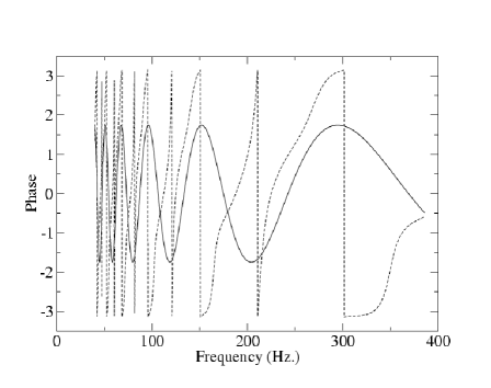
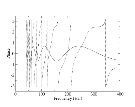
Figure 1: The dashed line on the left panel shows the phase modulation $\phi_{\rm mod}$ of the signal (Eq. (4)). The dashed line on the right panel shows the residual phase $\Delta\phi$ (Eq. (5)) after the first maximization over non-precessing parameters of the templates. The solid lines correspond to the best-fitting phase correction $\phi^{\rm cor}$ (Eq. (3)) when the non-precessing parameters are set equal to those of the signal (left panel) and when they are derived through a maximization process, leading to a mismatch (right panel). For more details see text. The physical configuration is $m_{1}=10M_{\odot}$, $m_{2}=1.4M_{\odot}$, $S=1$ and $\kappa=0.4$. The random angles are given by the first line of Table 1 (Configuration I).

The second configuration (II) differs qualitatively from the first one and exhibits clear oscillatory behavior in the phase modulation $\phi_{\rm mod}$ itself (Eq. (4)) (dashed line of the left panel of Figure 2). We can perform the same tests as with Configuration I. We fix the Newtonian parameters of the templates to those of the signal, and maximize over the three parameters of (3). It turns out that in this case the fit is quite good, and this maximization raises the FF from $0.21$ to $0.67$. However, in a real search, the non-precessing parameters are unknown, as we noted before. It turns out that the first maximization over the non-precessing parameters introduces a monotonic behavior ($\left[2\pi\right]$) to the residual phase $\Delta\phi$ (Eq. (5)) (dashed line on right panel). As a result the second maximization (this time over the three parameters of (3) does not lead to a high improvement of the ${\rm FF}$: from $0.55$ after the use of of the Newtonian templates it increases to to $0.67$ after the addition of (3). The fact that the two final ${\rm FF}$ are almost equal is fortuitous. Indeed, in Apost96 , Apostolatos made the assumption that the non-precessing variables ${\mathcal{M}}$ and $t_{c}$ are not correlated to the parameters of the correction (3). If this is the case, the ${\rm FF}$ obtained by doing the maximization in two steps is the same than the one that would be computed doing a five-dimensional search. The ${\rm FF}$ obtained by fixing the Newtonian parameters could only be smaller (or equal in this extreme case). From our computation, it seems that this uncorrelation is not as good as stated in Apost96 . However, this needs further exploration, beyond the scope of this paper.

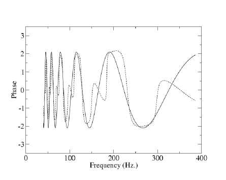
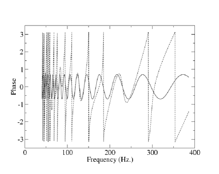
Figure 2: Same as Fig. 1 by for Configuration II.

The two previous examples illustrate the fact that the oscillatory correction proposed by Apostolatos does not recover the main part of the signal because the residual phase $\Delta\phi$ exhibits some kind of monotonic behavior, which is either inherent to the precession phase modulation (configuration I) or is introduced after the first-step maximization over the non-precessing parameters (configuration II). We have performed many more example studies like the above with consistent results, but of course this analysis does not constitute a proof. Given the very complicated dependence of the precession phase on a large number of parameters (some non-physical, e.g., orientation angles), it is difficult to imagine how one can derive an exact proof of the qualitative characteristics of the precessing inspiral signal. However, these example studies provided us with motivation for the development and the choice of a new template family that has been tested, increases FF values, and is presented next.

II.2 Spikes in the phase residuals

Our extensive study of specific precession waveforms helped us realize that the main features of Figures 1 and 2 are rather common. Indeed the monotonic behavior can be represented by a succession of spike-like structures centered further apart as frequency increases. The origin of the spikes in this representation of the phase (modulo $2\pi$) is related to the fact that the residual phase jumps from $0$ to $\pi$ and $0$ to $-\pi$ on either side of each spike. To reflect this rapid change in phase we choose a mathematical form with an infinite derivative at the central frequency of the spike $f_{0}$:

$$\mathrm{If}\quad f>f_{0}\quad\mathrm{then}\quad P\left(f_{0},\sigma,\varepsilon\right) = \varepsilon\pi\left[\sqrt{\left(1-\frac{1}{\left(\sigma\left(f-f_{0}\right)+1\right)^{2}}\right)}-1\right]$$ (6)

$$\mathrm{If}\quad f<f_{0}\quad\mathrm{then}\quad P\left(f_{0},\sigma,\varepsilon\right) = \varepsilon\pi\left[-\sqrt{\left(1-\frac{1}{\left(\sigma\left(f-f_{0}\right)-1\right)^{2}}\right)}+1\right].$$

The functions $P$ (Fig. 3) depend on three well constrained parameters :

• $\varepsilon$ is either $1$ or $-1$ and represents the two possible orientations of the spike.

• $\sigma$ is related to the width of the spike. More precisely the half width is $f_{1/2}=\left(2\sqrt{3}-3\right)/\left(3\sigma\right)$.

• $f_{0}$ is the central position of the spike.

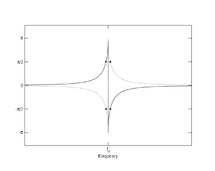
Figure 3: Function $P$. The solid line corresponds to $\varepsilon=1$ and the dotted line to $\varepsilon=-1$. The central position is $f_{0}$. A measure of the width of the spike is given by the black dots are located at half width, i.e. at $f_{0}\pm f_{1/2}$.

To recover most of the residual phase $\Delta\phi$ (Eq. (5)) (after the first-step maximization over non-precessing parameters has been performed), like those in the right panels of Figures 1 and 2, we need to account for a sequence of a few or several spikes. By definition, the functions $P$ represent narrow spikes, and hence their value is non-zero only very close to $f_{0}$. Thus, a sum of functions $P$, with a range of $f_{0}$, $\sigma$, and $\varepsilon$ values should give us a good representation of the qualitative behavior of residual phase with frequency. In principle, a prescription providing us with the number of spikes, their positions, and their width is needed. The main constraints are that (i) such prescriptions must depend on as few parameters as possible and (ii) they must recover the number and properties of spikes well enough to increase FF significantly. We tested various possible choices, but no accurate, simple prescription was found. The reason is rather obvious given the morphology of these features of the residual phase: the functions $P$ are strongly localized in frequency space, so that the positions $f_{0}$ must coincide very precisely with the location of the spikes in the residual phase.

If the problem is related to the fact that $P$ is a highly localized function, so does the solution. Indeed, given their behavior, it seems natural to assume that the various spikes do not influence each other very much. More precisely, the correction of one particular spike will not influence the properties of the others, precisely because the functions $P$ are non-zero only very close to their center frequency. This leads us to consider a hierarchical search, where spike after spike is identified sequentially. Each step in this sequence involves just a 2-parameter search ($f_{0}$ and $\sigma$; $\varepsilon$ only has two possible values and therefore can be taken into account explicitly by doubling the extent of the search in the other two parameters). We note that $\sigma$ is narrowly constrained, since the spikes of relevance are always very narrow (highly localized). Two-parameter searches are repeated until the relative change in FF drops below a certain threshold, typically $10^{-2}$.

However, we found that, in some cases, an oscillatory behavior can be present (e.g., configuration II in the previous subsection). Therefore it seems reasonable to keep the Apostolatos phase correction (3). Such maximization can “mimic” accurately most of oscillations in the residual phase (note, for example, the two bumps on the right panel of Fig. 2, around 125 and 220 Hz). Therefore a hierarchical set of the 2-parameter searches for the spikes must follow.

Depending on the behavior of the residual phase, three types of situations can be expected :

• The residual phase is oscillatory. In such a case a phase correction of the form (3) recovers most part of the signal and ${\rm FF}$ increases. Not many spikes, if any, are expected, and subsequent searches with the “spiky” templates do not improve ${\rm FF}$ (it is important to note that no computational effort is wasted with the spiky template searches, since those are aborted if the increase in ${\rm FF}$ is not significant).

• The residual phase contains both spikes and oscillations (e.g., right panel of Figure 2). Phase corrections (3) will trace the oscillations, and only moderately “pollute” the spikes. The hierarchical spike search is necessary and the ${\rm FF}$ increases substantially after both types of maximizations.

• The residual phase contains only spikes. The oscillator (3) does a really poor job (e.g., right panel of Figure 1) in recovering the signal-to-noise ratio. However, this first search for oscillatory corrections does not introduce significant spurious traces to the residual phase. Several spikes are found and lead to a significant increase of ${\rm FF}$.

These three types are rather simplistic in their description, but we have found that they cover the full range of possible situation at roughly equal weights, for the full range of random angles that determine the signal as “seen” by the detector.

Let us finally comment on the role of the oscillatory phase correction (3). It was initially motivated as a correction that will closely track the number of precession cycles (Eqs. (29) of Apost95 ). If this were true, the pulsation of the oscillation (expressed by ${\mathcal{B}}$) should lie close to the one given by Eqs. (29) of Apost95 . However, we found in Paper I that this is not the case, and that the values of ${\mathcal{B}}$ for which the maximum ${\rm FF}$ was obtained were very scattered. After careful examination of the behavior of the correction and the residual phases, we can confidently conclude that the reason for this unexpected uncorrelation is the fact that (3) can efficiently track any kind of bump in the phase. This realization can also explain the very weak dependence of the results on the specific form of the frequency dependence ( $f^{-2/3}$ or $f^{-1}$, cf. Sec. VI of Apost96 ): the bumps become wider as the frequency increases and this effect can be reflected in any decreasing function of $f$ multiplying ${\mathcal{B}}$ in (3).

II.3 The procedure and some examples

In the previous sections we used specific examples to probe in detail the main qualitative effects of precession on waveforms. The results of such an analysis motivated us to develop a new family of templates, which combined with the oscillatory form originally suggested by Apost96 can increase the FF to desired levels. In what follows we summarize our suggested complete procedure for searches of precessing inspiral signals, It involves three successive steps:

• A non-precessing Newtonian search using the standard 2-parameters chirp family SathyD91 ; DhuraS94 ; BalasD94 , where ${\mathcal{M}}_{\rm max}$ and $t_{\rm max}$ that maximize ${\rm FF}$ are determined. The phase of the associated template $T_{\rm max}$ is

  $$\phi_{\rm Newt}=2\pi t_{\rm max}f+\frac{3}{128}\left(\pi{\mathcal{M}}_{\rm max}\right)^{-5/3}f^{-5/3}+\phi_{\rm const}$$ (7)

  where $\phi_{\rm const}$ is a constant phase. It is well known that the maximization with respect to $\phi_{\rm const}$ is analytical, so that the search is really only two-dimensional. However let us mention that this phase can be computed and is used when plotting the various residual phases.

  We would like to mention that the maximization over $t_{c}$ can also be obtained, in a more computationally efficient way, using FFT techniques. In particular, such algorithms are used for current searches with LIGO. However, the version of the code used in this paper does not use this feature. Such an improvement of the code has now been implemented (after submission) and FFT will be used for future work. We note that the first tests show an almost perfect agreement between the FFT method and the one used for this paper ($<1\%$), and therefore it is not necessary to re-derive the results presented here and obtained by a grid-based method. However, the use of the FFT technique will allow us to explore a greater parameter-space.

  It is important to note that this step can be replaced by a PN search where the two compact object masses can decouple. We have adopted a Newtonian for reasons of computational efficiency, but we have shown (Paper I) that the results don’t change significantly as long that the order of the search in this first level is consistent with the order used to construct the non-precessing part of the signal. We will return to this issue in Sec. III.2 (see also Paper I; cf. Apost96 for effects of inconsistent choices).

• A three parameter search using the oscillatory correction (3) to the phase (7). The values that maximize FF are ${\mathcal{B}}_{\rm max}$, ${\mathcal{C}}_{\rm max}$, and $\delta_{\rm max}$, and the phase of the newly determined template is

  $$\phi_{0}=2\pi t_{\rm max}f+\frac{3}{128}\left(\pi{\mathcal{M}_{\rm max}}\right)^{-5/3}f^{-5/3}+\phi_{\rm const}+{\mathcal{C}}_{\rm max}\cos\left({\mathcal{B}}_{\rm max}f^{-2/3}+\delta_{\rm max}\right)$$ (8)

• The last step consists of identifying the spikes in the residual phase (8). The spikes are searched one by one, and for each one a 2-parameter search is performed (plus the boolean parameter $\varepsilon$). This sequential search ends when the relative change in ${\rm FF}$ is smaller than a given threshold. Let us call $N_{\rm max}$ the number of spikes found and $f_{0\,{\rm max}}\left(i\right)$, $\sigma_{\rm max}\left(i\right)$, and $\varepsilon_{\rm max}\left(i\right)$ the frequency positions, widths, and signs that maximize FF. The phase of the associated template $T_{\rm max}$ is

  $$\phi_{N_{\rm max}}= 2\pi t_{\rm max}f +\frac{3}{128}\left(\pi{\mathcal{M}_{\rm max}}\right)^{-5/3}f^{-5/3}+\phi_{\rm const}+{\mathcal{C}}_{\rm max}\cos\left({\mathcal{B}}_{\rm max}f^{-2/3}+\delta_{\rm max}\right)$$ (9)

  $$+ \sum_{i=1}^{N_{\rm max}} P\left(f_{0\,{\rm max}}\left(i\right),\sigma_{\rm max}\left(i\right),\varepsilon_{\rm max}\left(i\right)\right)$$

We note that nothing at this point ensures that this step-wise procedure produces the highest ${\rm FF}$ possible. We intend to perform tests and maximizations over combined template parameters (4 and 5-dimensional) in the near future, as our computational resources permit. However, we stress that the procedure suggested at this point involves a number of few-parameter, computationally efficient searches through template spaces. There is only one 3-dimensional search. In fact it seems that four-parameter searches are beyond current and near-future developments in computational resources VecchO02 .

In what follows we give one example of how the above procedure can increase the SNR and hence the detection rate. We use Configuration II from Figure 2, which combines both oscillatory and spiky behavior (second type of signal from the previous subsection). Figure 4 shows both the residual phase (i.e., the phase difference between the signal and the Newtonian best-fitting template) and the “mimic” phase at the end of the search procedure. In this particular case, the value of ${\rm FF}$ converges to 0.79 after seven spikes have been identified.

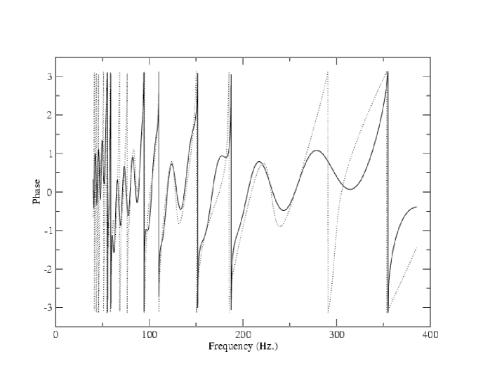
Figure 4: The dotted line is the residual phase $\Delta\phi$ (Eq. (5)), for the Configuration II (same as on the right panel of Fig. 2). The solid line shows the “mimic” phase of the template, i.e., the sum of Eq. (3) and seven spikes (6). The resulting FF is equal to 0.79. It is clear that the final “mimic” template matches the residual phase well.

The plots of Fig. 5 provide another way of examining the results. The first panel (top left) shows the phase of the signal (configuration II in Table 1). The second one (top right) shows the residual phase between the signal and the best-fitting Newtonian template, the third one (bottom left) the residual phase after the best fitting oscillatory form (3) is incorporated in the template, and the last one (bottom right) the residual after all seven spikes have been identified and included in the final template. Each step can be viewed as an attempt to reduce the phase difference to zero, i.e. to make the curves of Figure 5 as close to zero as possible. This particular example shows that our suggested procedure works very well, especially in the regions of maximum sensitivity around 150 Hz. Indeed the phase difference is drastically reduced in those regions. The remaining spikes have not been found because they cause a very small increase of the ${\rm FF}$, either because they are not very wide or because they are located at frequencies where the noise is high.

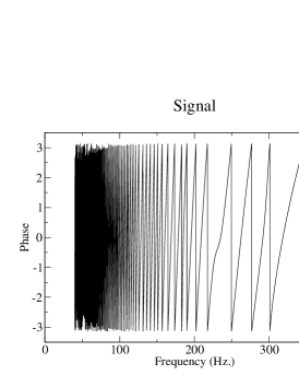
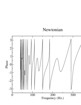
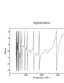
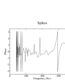
Figure 5: The top-left panel shows the phase of the signal for the Configuration II. The other plots show the residual phase after each step of the search procedure is completed: after Newtonian search (top right), oscillatory phase correction (bottom left), “spiky” phase correction (bottom right; seven spikes).

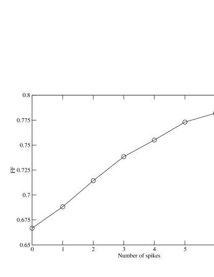
Figure 6: Convergence of the ${\rm FF}$ value as more and more spikes are added to the phase. The search was ended when the relative change in ${\rm FF}$ dropped below $10^{-2}$ (Configuration II).

Finally, in Figure 6 we show the improvement in FF as more and more spikes are identified and added to the best-fitting template. The case $n=0$ corresponds to the case where only the oscillatory term (3) is included. The curve shows that, indeed, the more efficient spikes (i.e. the ones giving rise to the best improvement in one step), are found first. This is a clear and strong indication of the independence of the spikes, which is crucial for the success of the hierarchical search. The curve converges as less and less significant spikes are identified and included. In this particular case, the ${\rm FF}$ using just Newtonian templates is $0.55$. Both the oscillatory correction and the spikes produce an improvement of about $20\%$. It is a case where both types of corrections are important. This is actually expected, as the residual phase (top right panel of Fig. 2) contains both bumps and spikes.

Let us mention that the previous example is by far not one of the best cases. In fact the final ${\rm FF}$ is somewhat smaller than the average value. One of the best case (out of 2,000 sets of random angles) is shown on Fig. 7. The left panel shows both the residual phase (dashed line) and the fit (solid line) after the finding of five spikes. The convergence of the ${\rm FF}$ is plotted on the right panel and it shows an impressive convergence to a value of almost $0.97$. The value using just the Newtonian templates is $0.78$.

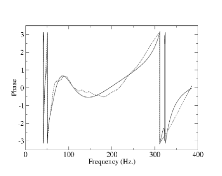
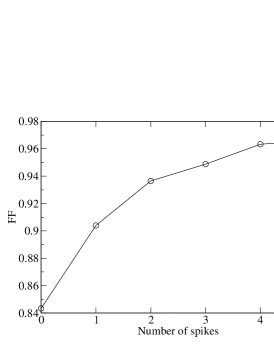
Figure 7: The left panel shows the residual phase (dashed line) and its fit including an oscillatory phase correction and five spikes (solid line). The right panel shows the convergence of the ${\rm FF}$ as more and more spikes are found. The physical parameters are $m_{1}=10\,M_{\odot}$, $m_{2}=1.4\,M_{\odot}$, $S=1$ and $\kappa=0.4$. The random angles are given by $\cos\theta=-0.632$, $\varphi=2.57$, $\cos\theta^{\prime}=0.593$, $\varphi^{\prime}=5.65$ and $\alpha_{\rm prec}=5.67$.

II.4 Other possible corrections

So far we have focused on an empirical approach that aims at reducing the phase difference between the signal and the best possible template. Indeed, matched-filtering techniques require that signal and template be in phase for the longest possible frequency. Therefore one might expect that phase corrections are more crucial than amplitude modulations. Once the suggested procedure is completed, the residual phase appears to be very noisy (e.g., bottom-right panel of Figure 5). It seems to us that it is almost impossible to find any additional systematic correction. However, in an attempt to further increase the ${\rm FF}$ value, we examine whether a correction to the amplitude of the templates would be useful.

The amplitude modulation ${\rm AM}$, in the simple precession regime, is mainly oscillatory (Eq. (11) of Apost95 ). So it is natural to introduce an amplitude correction with the same form as Eq. (3). Given that ${\rm FF}$ is independent of the absolute normalization, we can drop the parameter ${\mathcal{C}}$ this time. Then we are left with the following correction:

$${\mathcal{A}}^{\rm cor}=\cos\left({\mathcal{B}}^{\rm ampli}f^{-2/3}+\delta^{\rm ampli}\right).$$ (10)

One must then determine the appropriate way to include such a correction. One simple way is to apply it sequentially after all the corrections to the phase (described above) have been applied. We have tested such an approach and found almost no improvement at all in terms of increasing ${\rm FF}$. We conjecture that the mismatch of the non-precessing parameters and all the modifications on the phase have already attempted to “mimic” the amplitude modulation. Alternatively we attempt to apply the amplitude correction (10) before any phase corrections except for the Newtonian search. We decide to combine the amplitude correction with the search with respect to the non-precessing parameters in one single, four-dimensional maximization, by using the following template

$$\tilde{h}\left(f\right)={\mathcal{A}}^{\rm cor}f^{-7/6}\exp\left(i\phi_{\rm Newt}\right)$$ (11)

where $\phi_{\rm Newt}$ is given by Eq. (7), so that the template (11) is just the Newtonian template corrected by an oscillatory term in the amplitude. Once this first step is completed, we follow with the standard procedure of phase corrections, starting with the oscillatory term and following with the spikes.

The first maximization mentioned above is four-dimensional, and hence computationally demanding. Therefore we restrict it to a few sets of random angles, typically ten. For each configuration, we calculate the associated ${\rm FF}$ by using both the standard procedure (without any amplitude corrections) and the four-dimensional search (followed by the oscillatory and “spiky” searches). Clearly exploring just 10 sets of random angles is not adequate but it can still indicate whether the amplitude correction is important or not.

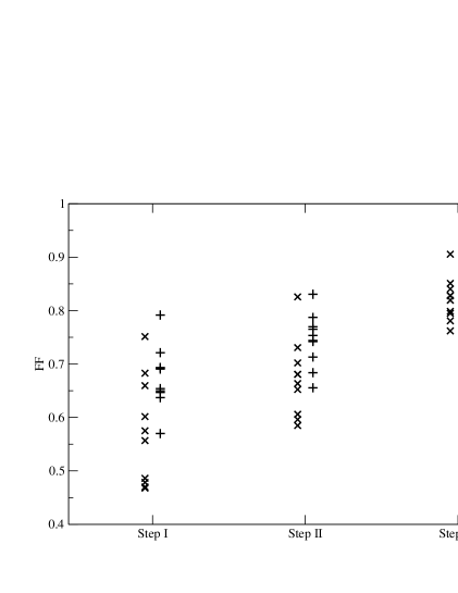
Figure 8: Comparison between the standard method ( $\times$ symbols) and the method including an amplitude correction ( $+$ symbols). For $m_{1}=10$ M_⊙, $m_{2}=1.4$ M_⊙, $S=1$, and $\kappa=0$, ten sets of random angles are shown (some of the points overlap).

Figure 8 shows the comparison for ten values of the random angles, for $m_{1}=10$ M_⊙, $m_{2}=1.4$ M_⊙, maximum spin magnitude ($S=1$), and a spin-tilt angle of 90 degrees ($\kappa=0$). Each symbol denotes the value of ${\rm FF}$ for one particular orientation (some points are not visible due to overlap). The $\times$ symbols correspond to results for the standard procedure and the $+$ symbols to those from the four-dimensional search. Between the two procedures, only Step I is different; Step II is the search for oscillatory corrections (3), and Step III is the search for spikes. We find that initially the four-dimensional search leads to higher ${\rm FF}$ values in comparison to the Newtonian and oscillatory search, but this effect is overcome by the inclusion of spikes. At the end of the process, the average fitting factor is almost the same for the two methods : $<{\rm FF}>=0.821$ for the standard procedure and $<{\rm FF}>=0.828$ for the case with the amplitude correction. Given these tests, we conclude that no significant gain seems to be associated with the inclusion of an amplitude modulation to the template family.

Even though $<{\rm FF}>$ values are very close, the procedure involving the more computationally demanding four-dimensional search might still be a viable choice, if, for example, the extraction of the physical parameters of the binary is more accurate. To examine this question, we compare the parameters of the signal (${\mathcal{M}}\simeq 2.99M_{\odot}$ and $t_{c}=0$) to the best-fitting values obtained with the two different methods. We focus on the chirp mass and show the results in Figure 9. It is clear that the dispersion around the signal-value of the chirp mass is very comparable for the two methods. We have conducted tests for $m_{1}=7$ M_⊙, $m_{2}=3$ M_⊙, $S=1$, and $\kappa=0.4$ and observed very similar behaviors. Therefore, at this point, it seems that there is no good reason for using the time-consuming four-parameter search instead of the standard method described earlier.

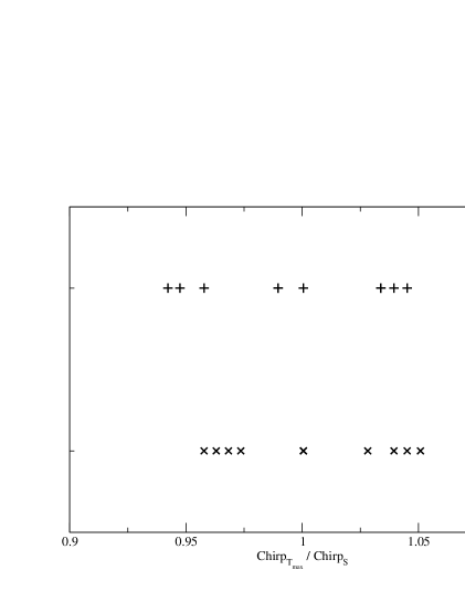
Figure 9: Range of estimated chirp masses, measured by the ratio of the estimated values (i.e. the ones of the template for which the maximum ${\rm FF}$ is attained) to the “true” values (i.e. the ones of the signal). The sets of random angles and the physical parameters are the same than the ones of Fig. 8. The $\times$ denote the standard method and the $+$ the four-dimensional search.

III Efficiency of the “spiky” templates

III.1 Determination of the computational parameters

To perform the searches we need to first determine a number of computational parameters: the boundaries of the parameter space to be searched (we do make use of our knowledge of the true parameters of the signal), the number of templates between these boundaries, the number of sets of random angles needed to obtain an accurate average $<{\rm FF}>$, the number of collocation points needed to obtain an accurate value for ${\rm FF}$ with a Gauss-quadrature scheme used in the cross-correlation calculations.

In what follows we briefly illustrate how the search intervals are found, using the chirp mass as an example. We first determine the values ${\mathcal{M}}_{\rm min}$ and ${\mathcal{M}}_{\rm max}$, so that the maximum value of the ${\rm FF}$ is always obtained for a value ${\mathcal{M}}_{\rm max}$ inside this range. Of course, for reasons related to computational time, we would like to search through intervals as small as possible. To determine the limits, for each choice of masses, we consider one of the worst cases for the ${\rm FF}$, that is $S=1$ and $\kappa=-0.5$ (see results of Paper I, for why this is the worst case). For this orientation, we use a very broad interval for the search of the maximum. Fig. 10 shows the histogram of the occurrences at which the maximum of the ${\rm FF}$ is obtained at a given ${\mathcal{M}}_{\rm max}$, for $m_{1}=10M_{\odot}$, $m_{2}=1.4M_{\odot}$, $S=1$ and $\kappa=-0.5$. In this particular, example the search interval is then chosen to be $\left[0.8{\mathcal{M}}_{s},1.3{\mathcal{M}}_{s}\right]$, where ${\mathcal{M}}_{s}$ is the chirp mass of the signal (less than $1\%$ of the maxima lie outside this range, for the particular realization of Fig. 10).

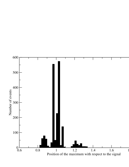
Figure 10: For 2,000 sets of random angles, the value of ${\mathcal{M}}_{\rm max}$ at which the maximum of the ${\rm FF}$ is attained, is computed and the results plotted in this histogram. The configuration is $m_{1}=10M_{\odot}$, $m_{2}=1.4M_{\odot}$, $S=1$ and $\kappa=-0.5$. The range of the plot is the actual range for the large search of the maximum (i.e. $\left[0.6{\mathcal{M}}_{s},2{\mathcal{M}}_{s}\right]$)

As we did in Paper I, the number of templates, sets of random angles, and collocation points are determined by studying the relative convergence of the ${\rm FF}$ as these numbers increase. Here we skip the details, but we mention that the chosen numbers are sufficient to ensure an accuracy of the ${\rm FF}$ calculation of 1% or better. We also require that for signals without any precession modulation we recover ${\rm FF}\geq 0.97$ Let us mention that we impose the convergence of ${\rm FF}$ for every configuration and not of the average $<{\rm FF}>$, which is a stronger constraint. This true for all computational parameters, except for the number of sets of random angles, for which only the convergence of the average $<{\rm FF}>$ makes sense. For example, Fig. 11 shows the relative convergence with the increasing number of collocation points $N$ used to calculate the integrals in the expression of the ${\rm FF}$. From this particular plot, we estimated that we should use 1,000 collocation points to get a relative error of order $10^{-3}$.

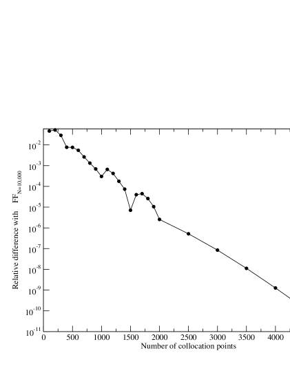
Figure 11: Convergence of the ${\rm FF}$ with respect to the number of collocation points. The signal is for $\left(10;1.4\right)$ solar masses objects, maximum spin and $\kappa=-0.2$. The random angles are $\theta=0.107\pi$, $\varphi=0.292\pi$, $\theta^{\prime}=0.412\pi$, $\varphi^{\prime}=1.85\pi$ and $\alpha_{\rm prec}=0.499\pi$. The comparison is done with the value for very high $N$ which is ${\rm FF}\simeq 0.46$.

The complete set of computational parameters used in our searches are summarized in Table 2. We also note that the grids associated with the masses are in logarithmic scale to ensure proper distribution of the templates.

Table 2: Various computational parameters for the (post)-Newtonian templates. The mass intervals are given in fraction of the signal masses. “Col” is the number of collocation points and “Angles” the number of sets of random angles. Let us mention that the parameters related to $t_{c}$ have no meaning when FFT techniques are used.

Masses $\left(M_{\odot}\right)$	Col	Angles	Interval ${\mathcal{M}}$	Number ${\mathcal{M}}$	Interval $t_{c}$ $\left({\rm s.}\right)$	Number $t_{c}$	Interval $m_{\rm T}$	Number $m_{\rm T}$
$\left(7;3\right)$	$1,000$	$2,000$	$\left[0.9;1.15\right]$	$90$	$\left[-0.05;0.05\right]$	$70$	$\left[1;2.4\right]$	$20$
$\left(10;1.4\right)$	1,000	2,000	$\left[0.8;1.3\right]$	$90$	$\left[-0.1;0.1\right]$	$130$	$\left[0.5;2.6\right]$	$30$

The computational parameters for the addition of Apostolatos’ correction are given in Tab. 3 and the ones for the spikes in Table 4. For each spike, $f_{0}$ is searched in all the range of frequency, from the low-cut at 40 Hz to the termination frequency at the ISCO. The value of the ISCO is the one of a test particle orbiting a Schwarzschild black hole. It may seem a rather crude approximation but, because the noise is high at those frequencies, its exact value is not expected to be important. A logarithmic grid is used for $f_{0}$, because the spikes are more densely distributed at low frequencies. We search for spikes until the relative change of fitting factor is smaller than $\delta{\rm FF}=10^{-2}$.

Table 3: Various computational parameters for the mimic templates.

Masses $\left(M_{\odot}\right)$	Interval ${\mathcal{B}}$	Number ${\mathcal{B}}$	Interval ${\mathcal{C}}$	Number ${\mathcal{C}}$	Interval $\delta$	Number $\delta$
$\left(7,3\right)$	$\left[0,75\right]$	30	$\left[0,\pi\right]$	10	$\left[0,2\pi\right[$	20
$\left(10,1.4\right)$	$\left[0,160\right]$	580	$\left[0,\pi\right]$	10	$\left[0,2\pi\right[$	10

Table 4: Computational parameters for the search of the spikes.

Masses $\left(M_{\odot}\right)$	Interval $f_{0}$	Number $f_{0}$	Interval $\sigma$	Number $\sigma$	$\delta{\rm FF}$
$\left(7;3\right)$	$\left[40;440\right]$	$500$	$\left]0;0.8\right]$	100	$10^{-2}$
$\left(10;1.4\right)$	$\left[40;386\right]$	400	$\left]0;0.8\right]$	60	$10^{-2}$

III.2 Results

In Figure 12 we show the efficiency of the “spiky” templates for $m_{1}=10$ M_⊙, $m_{2}=1.4$ M_⊙, and $S=1$. The left panel shows the average $<{\rm FF}>$ as a function of the cosine of the misalignment angle $\kappa\equiv\vec{S}\cdot\vec{L}$ and the right panel the reduction factor in detection rate $<{\rm FF}>^{3}$, assuming a uniform volume distribution of sources. It is evident that the new family of template can greatly improve the signal-to-noise ratio. Values of $<{\rm FF}>$ are above 0.8 for the full range of spin-misalignment angles. Consequently the reduction factors of detection rate increase by factors of up to 5-6 (compared to cases where precession is ignored; see Paper I) or in other words the detection rate is never reduced by more than a factor of 2. This is to be compared with the curves showing the Newtonian and Apostolatos’ templates for which the detection rate can be reduced by as much as 10 and 5 (respectively).

The triangles are computed by including 2PN corrections to the phases of the non-precessing parts of both the signal and the templates. As already stated in Sec. II.3, the results are almost the same as the ones obtained by using only Newtonian expressions. It is a clear validation of our results, as it illustrates the fact, already observed in Paper I, that the order of the non-precessing part is not important, as long as the order of the non-precessing parts is kept consistent between the signal and the templates.

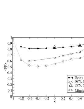
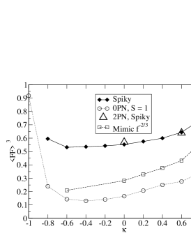
Figure 12: Efficiency of the “spiky” templates in recovering the signal-to-noise ratio and increasing the inspiral detection rate. The circles and dotted lines correspond to the values obtained using the Newtonian templates. The squares and dashed lines correspond to Apostolatos’ waveforms alone, and the filled diamonds and solid lines correspond to the combination of the Apostolatos’ and “spiky” templates. The triangles denote the values obtained by using 2PN order expressions for the non-precessing part for both the signal and the templates. The left panel shows the average $<{\rm FF}>$ whereas the right panel shows the reduction factors of the detection rate, both as a function of the cosine of the spin-misalignment angle.

Figure 13 shows the same results but for $m_{1}=7\,M_{\odot}$ and $m_{2}=3\,M_{\odot}$. The reduced detection rate $<{\rm FF}>^{3}$ is always greater than 70%, whereas it could drop to 50% if one uses only Apostolatos’ correction.

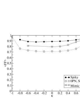
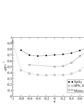
Figure 13: Same as Fig. 12 but for $m_{1}=7\,M_{\odot}$ and $m_{2}=3\,M_{\odot}$ (except for the 2PN triangles).

Figure 14 presents another way of looking at the improvement caused by the “spiky” templates. For $m_{1}=10\,M_{\odot}$, $m_{2}=1.4\,M_{\odot}$, $S=1$ and $\kappa=0.4$, the ${\rm FF}$ for 2,000 sets of random angles has been computed. Figure 14 shows the associated histogram, i.e. the number of configurations for which a given ${\rm FF}$ is obtained. One can clearly see that, after each step of our search procedure, (i) the $<{\rm FF}>$ increases and (ii) the distribution of ${\rm FF}$ values narrows significantly.

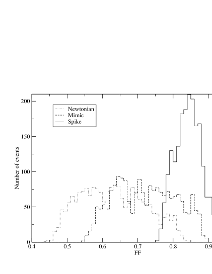
Figure 14: Distribution of ${\rm FF}$ values using 2,000 configurations (sets of random angles). The physical parameters adopted for the signal are $m_{1}=10M_{\odot}$, $m_{2}=1.4M_{\odot}$, $S=1$ and $\kappa=0.4$. The dotted line denotes the values after the use of the Newtonian templates, the dashed line those obtained after the addition of the Apostolatos’ oscillatory correction, and the solid curve those after all the important spikes have been identified.

As already stated in Sec. II.3, FFT techniques can also be used to compute the $<{\rm FF}>$ during the first step of our procedure (post-Newtonian search). Although such algorithms have not been used for obtaining the plots shown in this paper, we conducted a few tests to check the validity of our results. As expected, we found that the agreement between the two methods is almost perfect. Indeed, it is better than a fraction of $1\%$ for reasonable number of points used to compute the FFT.

IV Summary and Conclusions

The goal of this paper has been to find a new family of templates for the efficient detection of precessing binary inspiral. We are motivated by a careful study of the qualitative behavior of the residual phase once the signal has been matched with a best-fitting non-precessing template. This initial study provides with an explanation for the insufficiency of the purely oscillatory phase correction shown in Eq. (3), suggested for the first time by Apostolatos Apost96 . The problem seems to be that the mismatch between the non-precessing parameters of the signal and the templates fails to remove all the monotonic behavior of the phase modulation (cf. Fig. 1). In some other cases, the mismatch can even “pollute” the phase modulation and becomes responsible for the appearance of a monotonic component (cf. Fig. 2).

To tackle this problem, we have shown that the monotonic behavior of the phase can be represented by a succession of spike-like structures. These spikes can be searched very efficiently by using a hierarchical algorithm, in which the spikes are found one after the other until the ${\rm FF}$ converges. We note that, before searching for the spikes, it is useful to still use the oscillatory correction Apost96 because the oscillator (3) can account for any periodic behavior present in the residual phase. We also considered including a correction to the amplitude, in the form of an oscillator similar to Eq. (3). Our preliminary examination of this question did not reveal any significant improvement of the signal-to-noise ratio and therefor this approach did not warrant any further exploration.

Quantitative results about the usefulness of the “spiky” templates in improving detection rates have been presented, studying two configurations for which precession is most important ($\left(m_{1},m_{2}\right)=\left(10,1.4\right)$ and $\left(7,3\right)$ M_⊙). We find that, even in the most unfavorable cases, the detection rate is reduced by less than a factor of 2. This is to be compared with the factor of 10 reduction when precession is ignored altogether and the factor of 5 when the Apostolatos’ oscillatory correction is included.

We view our results as very encouraging, especially when one considers the very moderate number of parameters involved (two for each spike). Of course, it must be possible to obtain higher ${\rm FF}$ by using templates with more parameters, but the applicability to real searches may be problematic in terms of the associated computational efficiency. In our effort to find this new family of templates, keeping the number of parameters as low as possible was one of the main priorities, as long as the improvement in the detection rate is satisfactory.

In this study we focused on trying to quantify the efficiency of the newly proposed template family in increasing the SNR. For the immediate future there are a number of issues that we would like to examine in more detail, as our computational resources permit. The ultimate question is whether the “spiky” family of templates and the search procedure described here can be used in real searches.

As the very first step, we would like to examine this family’s efficiency when we move away from the approximations of simple precession and we consider more complicated precession signals, obtained by numerical integration of more complete post-Newtonian dynamics for example Kidde95 . We expect that the results will not change dramatically because of the generic nature of our family of templates. Indeed, the procedure presented in this paper should reproduce rather accurately any superposition of oscillatory (Apostolatos’ ansatz) and monotonic (the spikes) behaviors in the phase. Moreover, we found that the results did not change very much when higher order PN-effects were included in the non-precessing part (cf. Sec. III.2). Low false alarm rates and moderate numbers of templates needed for real searches are amongst the other properties that must be asserted. Issues related to reliable physical parameter estimation are also important, if we want to think about questions of interest to gravitational-wave astrophysics that goes beyond detection. We plan to conduct these studies in the near future and implement the “spiky” templates in LIGO algorithm library (LAL) LAL , should they constitute a viable family.

- (1) P. Grandclément, V. Kalogera and A. Vecchio, Phys. Rev. D, submitted, gr-qc/0207062 (2002) (Paper I).
- (2) T.A. Apostolatos, Phys. Rev. D 54, 2421 (1996).
- (3) A. Abramovici et al., Science 256, 325 (1992).
- (4) B. Caron et al., Nucl. Phys. B54, 167 (1997).
- (5) K. Danzmann, in Gravitational Waves Experiments, eds. E. Coccia, G. Pizzella and F. Ronga, World Scientific, Singapore (1995).
- (6) H. Tagoshi et al., Phys. Rev. D. 63, 062001 (2001).
- (7) C.W. Helstrom, Statistical Theory of Signal Detection, 2nd edition, Pergamon Press, London (1968).
- (8) B.J. Owen and B.S. Sathyaprakash, Phys. Rev. D 60, 022002 (1999).
- (9) L.S. Finn, Written version of lectures given at XXVI SLAC Summer Institute on Particle Physics Gravity: From the Hubble Length to the Planck Length, gr-qc/9903107, (1998).
- (10) C. Cutler and K. S. Thorne, An Overview of Gravitational-Wave Sources, to appear in Proceedings of GR16 (Durban, South Africa, 2001), gr-qc/0204090.
- (11) P.R. Brady, J.D.E. Creighton and K.S. Thorne, Phys. Rev. D 58, 061501 (1998).
- (12) A. Buonanno, Y. Chen and M. Vallisneri, Phys. Rev. D submitted, gr-qc/0205122 (2002).
- (13) T.A. Apostolatos, C. Cutler, G.J. Sussman and K.S. Thorne, Phys. Rev. D 49, 6274 (1994).
- (14) T.A. Apostolatos, Phys. Rev. D 52, 605 (1995).
- (15) B.S. Sathyaprakash and S.V. Dhurandhar, Phys. Rev. D 44, 3819 (1991).
- (16) S.V. Dhurandhar and B.S. Sathyaprakash, Phys. Rev. D 49, 1707 (1994).
- (17) R. Balasubramanian and S.V. Dhurandhar, Phys. Rev. D 50, 6080 (1994).
- (18) B. Owen and A. Vecchio, in progress.
- (19) L.E. Kidder, Phys. Rev. D 52, 821 (1995).
- (20) LIGO/LSC Algorithm Library Home Page : http://www.lsc-group.phys.uwm.edu/lal/