Gravitational waves from black hole binary inspiral and merger:
The span of third post-Newtonian effective-one-body templates

Abstract

We extend the description of gravitational waves emitted by binary black holes during the final stages of inspiral and merger by introducing in the third post-Newtonian (3PN) effective-one-body (EOB) templates seven new “flexibility” parameters that affect the two-body dynamics and gravitational radiation emission. The plausible ranges of these flexibility parameters, notably the parameter characterising the fourth post-Newtonian effects in the dynamics, are estimated. Using these estimates, we show that the currently available standard 3PN bank of EOB templates does “span” the space of signals opened up by all the flexibility parameters, in that their maximized mutual overlaps are larger than 96.5%. This confirms the effectualness of 3PN EOB templates for the detection of binary black holes in gravitational-wave data from interferometric detectors. The possibility to drastically reduce the number of EOB templates using a few “universal” phasing functions is suggested.

I Introduction

Current theoretical understanding, stemming both from general relativity and astrophysics, places black hole binaries at the top of the list of candidate sources for the interferometric gravitational-wave detectors that are nearing the completion of their construction phase. On the one hand, black hole binaries are by far sources whose dynamics (early inspiral and late time quasi-normal mode ringing to a large extent, late inspiral, plunge and merger to a lesser extent) is better understood than other sources, such as supernovae or relativistic instabilities in neutron stars, so that it is possible to construct reasonably good template waveforms to extract signals out of noise. On the other hand, astrophysical rate estimates of black hole binary coalescences, though not known accurately, have a range whose upper limit is large enough to expect a few mergers per year within a distance of 150 Mpc glpps .

The merger phase of binaries consisting of two $15M_{\odot}$ black holes takes place right in the heart of the LIGO-VIRGO-GEO sensitivity band giving us the best possible picture of this highly non-linear evolution. Eventually, when detectors reach good sensitivity levels, one hopes to learn experimentally about this strong gravity regime which has been a subject of intense analytical and numerical studies for more than a decade. In the meantime, what is needed is a set of model waveforms or templates that describe the dynamics close to the merger phase accurately enough so that only a small fraction $(<10\%)$ of all events will go undetected.

Two general viewpoints are possible to reach this goal. A maximalist one or a minimalist one. The maximalist viewpoint consists in enlarging as much as is conceivable (using in a “democratic” way all available methods in the literature for treating binary coalescence) the bank of filters, with the hope that even the methods which appear a priori less reliable than others might, by accident, happen to describe a good approximation to the “real” signal. This is the viewpoint taken by Buonanno, Chen and Vallisneri in their careful, and detailed analysis in Ref. BCV02 , on the basis of which they advocate expanding the net by using a multiparameter template family able to approximate most of the results of the conceivable analytical methods. However, this “democratic” attitude comes at a cost that calls for an alternate strategy that we explore here. The problem with this method is that it leads to a dramatic increase in the total number of templates from $\sim 25$ templates to $\sim 10^{4}$ templates; which has the bad consequence that it leads a larger false alarm rate. (These estimates of the number of templates are those obtained, as in BCV02 , by “dividing” the parameter space by the local span of the template at the minimal match. This is an underestimate because it neglects boundary effects. For instance, a more realistic estimate of the number of the third post-Newtonian effective-one-body templates would be $\sim 150$ rather than 25.)

By contrast, we advocate here a minimalist viewpoint consisting in (i) focussing exclusively on the best available analytical description, and (ii) generalizing this description by adding several parameters that describe “new directions” corresponding to physical effects not perfectly modelled by this description. The most important of these directions are the effects due to higher post-Newtonian (PN) effects, not yet calculated, but known to exist. A thorough study of the robustness of our preferred description against the inclusion of currently unknown effects should allow an informed and judicious covering of the parameter space of interest without overtly expanding the size of the total bank of templates.

The best available analytical description at present is, in our opinion, the “effective-one-body” (EOB) approach proposed and constructed for non-spinning bodies at second post-Newtonian (2PN) order by Buonanno and Damour BD99 ; BD00 , extended to third post-Newtonian (3PN) order by Damour, Jaranowski and Schäfer DJS00 and generalized to spinning bodies by Damour TD02 . On the one hand, the EOB maps, using the Hamilton-Jacobi formalism, the real “conservative” (in the absence of radiation reaction) dynamics of two bodies with masses $m_{1}$ and $m_{2}$ into an EOB problem of a test particle of mass $\mu\equiv{M\eta}$ (where $M\equiv{m_{1}+m_{2}}$ and $\eta\equiv{m_{1}m_{2}/M^{2}}$), moving (essentially) in an effective background metric $g_{\mu\nu}^{\rm eff}$ which is a deformation of the Schwarzschild metric with deformation parameter $\eta$. Further, by supplementing the above dynamics by an additional radiation-reaction force obtained from a Padé resummation of the gravitational-wave flux, it allows for the first time the possibility to go beyond the adiabatic approximation and to analytically discuss the transition from inspiral to plunge and the subsequent match to merger and ringing. The implications of the EOB templates for data analysis of binary black holes were explored in DIS3 where it was shown that the signal-to-noise ratio (SNR) is significantly enhanced relative to the usual PN templates due to inclusion of the plunge signal. The EOB formalism does also provide initial dynamical data (position and momenta) for two black holes at the beginning of the plunge to be used in numerical relativity to construct gravitational data like metric and its time derivative and evolve Einstein’s full equations through the merger phase.

The analytical prediction of the EOB method (including spin) for invariant functions were compared to numerical results based on the helical Killing vector approach BGG02 for circular orbits of corotating black holes by Damour, Gourgouhlon and Grandclément DGG02 and shown to agree remarkably well. The agreement was robust against choices of resummation of the EOB potential and improved with the PN order. Recently, Buonanno, Chen and Vallisneri BCV02 made a detailed and exhaustive comparison of all currently available waveforms for non-spinning binary black holes resulting from different approximations. This study showed (among other results) that EOB models are more reliable and robust than other non-adiabatic models.

Recently Blanchet B02a has made a comparison of the straightforward PN predictions with BGG02 and shown that at 3PN order they are as close to the numerical results as the resummed approaches. While it is indeed interesting to note this closeness of the results derived from one particular non-resummed 3PN function (the “energy function” $E(\omega)$ for circular orbits) to the numerical results (and to the EOB ones), we still do not see any way yet by which, as the Hamiltonian $H({\bf r},{\bf p})$ does in the EOB approach, the bare PN results for the “ circular energy function” $E(\omega)$ can be used to define templates beyond the adiabatic approximation. As Ref. BD00 has shown the importance of going beyond the adiabatic approximation in describing the smooth transition between the inspiral and the plunge, and as DIS3 ; BCV02 has shown how significant was the contribution of the plunge to the SNR, we consider that the EOB waveforms are the best, currently available, analytical templates for binary black hole coalescences.

In this paper, we wish to strain to extremes the flexibility of the EOB formalism by tugging it in directions where it can be theoretically pulled and by locating directions it is most likely to yield under deformations by unmodelled effects (including higher order PN effects). We shall introduce seven “flexibility” directions i.e.  seven new flexibility parameters. Then we will investigate the “span” of the original (3PN) EOB templates in the space of waveforms opened up by our extension of the EOB waveforms into seven new “flexibility” directions. By span of a given bank of templates, we mean the region of signal space which is well modelled by some template in the bank, i.e.  the set of signals $S$ such that the maximized overlap of $S$ with some template $T$ is larger than 0.965 . Among our seven flexibility parameters, some like $b_{5}$ represent higher order (fourth post-Newtonian, 4PN) corrections in the dynamics, some like $\theta$, the arbitrariness in the best available 3PN gravitational-wave flux calculation due to incompleteness of the Hadamard partie finie regularization, and others like $c_{P}$ denote a parameter used to factor the gravitational-wave flux in DIS1 and accelerate the convergence of the Padé approximants to the numerical flux in the test-mass case. Further, the current development of EOB has made, at several stages, specific choices of representation of various physical effects and, as in any analytical construction, the choices were the simplest that one could apparently make. We then explored the effects induced by a modification of these simple choices, i.e.  the consideration of new versions of EOB, characterised by different parameter values reflecting other allowed more complex choices. These comprise the remaining four parameters and include $z_{2}$($\zeta_{2}$) a parameter appearing in the effective Hamiltonian $H_{\rm eff}$ of the EOB, $f_{\rm NonAdiab}$, a parameter to modify the simplest treatment of non-adiabatic effects in the current version of EOB templates; $f_{\rm NonCirc}$, a parameter to modify the simplest treatment of non-circular effects in the current version of EOB templates and finally $f_{\rm transition}$ to allow the possibility that the transition between plunge and ringing may occur at frequencies different from that assumed in the simplest EOB model. The seven parameters $(b_{5},\,\theta,\,c_{P},\,\zeta_{2},\,f_{\rm NonAdiab},\,f_{\rm NonCirc},\,f_{\rm transition})$, are referred to as the flexibility parameters. Varying them and testing the change of the physical predictions under reasonable variation of these parameters is a way of probing the overall robustness of the EOB framework. What we specifically investigate is whether a bank of standard 3PN EOB templates is sufficient to represent all plausibly relevant extended family of waveforms generated by these new flexibility parameters.

In the context of this investigation our waveforms will be parameterized by two sets of parameters: (a) The first set consists of the usual intrinsic and extrinsic parameters entering the construction of standard waveforms, such as the masses of the component objects and their spins, some reference phase, etc., denoted collectively by $p_{k},$ $k=1,\ldots,K.$ In this work we shall only deal with non-spinning point-particles in the restricted PN approximation cutleretal93a which requires $K=4$ with $p_{1,2}=m_{1,2}$ denoting the masses of the two bodies, $p_{3}=t_{\rm ref}$ a reference time (related to the instant of coalescence), and $p_{4}=\Phi_{0}$ the phase of the wave at the reference time. (b) The second set consists of the flexibility parameters introduced above. We shall denote these flexibility parameters as $\pi_{a},$ $a=1,\dots,A,$ with ($A=7$)

$$\pi_{1} = b_{5},\ \ \pi_{2}=\theta,\ \ \pi_{3}=c_{P},\ \ \pi_{4}=z_{2}(\zeta_{2}),\ \$$

$$\pi_{5} = f_{\rm NonAdiab},\ \ \pi_{6}=f_{\rm NonCirc},\ \ \pi_{7}=f_{\rm transition}.$$ (1)

For studies of the span of a bank of templates of the kind we propose to do in this paper, it is helpful to introduce the notions of a standard or fiducial template and its associated variant or flexed signal constructed by turning on one of the flexibility parameters. The term fiducial template is used to represent a waveform constructed in a certain approximation and at a given PN order with a fixed set of values of the unknown parameters introduced above. In this paper, our fiducial template will be the standard EOB waveform (see Sec. III) at the 3PN order with the flexibility parameters all set to zero:

$$\text{Fiducial Template}=h(t;p_{k},\pi_{b}=0,\forall b)\equiv T(t;p_{k}).$$ (2)

In contrast, the associated flexed signal will again be the EOB waveform at 3PN order with all but one of the flexibility parameters $\pi_{a}$ set to zero:

$$\pi_{a}\text{-Flexed Signal}=h(t;p_{k},\pi_{a}\neq 0,\pi_{b}=0,\forall\ b\neq a)\equiv S(t;p_{k},\pi_{a}).$$ (3)

In other words, in our test of robustness we do not allow all the seven parameters to vary simultaneously. Such a variation would lead to a formidably high dimensional parameter space which is computationally impossible to investigate at the moment. Rather, our aim is to study the effect of each flexibility parameter independently and to gauge the extent to which our standard fiducial template waveform can mimic the changes brought about by the flexibility parameters $\pi_{a}$ by a mere variation of the intrinsic parameters $p_{k}$. Such a systematic study allows us to isolate and identify the most important unknown physical effects, and decide if it is necessary to introduce the corresponding flex parameter as an additional parameter in search templates used in the detection of gravitational waves from black-hole binaries.

As in earlier work, our main tool for measuring the span of a bank of templates is the overlap of a standard fiducial template with a given flexed signal. (See Sec.VI for the definition of the overlap.) In this study, we use two measures of “good overlaps”: faithfulness and effectualness DIS1 . A template is said to be faithful if its overlap with a flexed signal waveform of exactly the same intrinsic parameter values is larger than 0.965 (after maximization over the extrinsic parameters). It is expected that faithful templates are also good at estimating source parameters although this is not guaranteed to be the case. A template is said to be effectual if its overlap with a flexed signal waveform, maximized over all the intrinsic and extrinsic parameters, is larger than 0.965. Obviously, every faithful template is necessarily effectual but not all effectual templates are faithful. Note that the notions of faithfulness and effectualness might depend on the particular flexibility direction which is explored: While a template waveform could be faithful with respect to the $\pi_{1}$-flexed signal, it might only be effectual with respect to the $\pi_{2}$-flexed one and neither with respect to the $\pi_{3}$-flexed one.

Implementing the above analysis we conclude that the standard 3PN EOB templates are effectual with respect to all flexibility parameters introduced in this study including the parameter $b_{5}$ characterising the 4PN dynamical effects. In other words, the span of the bank of 3PN EOB templates is large enough to cover the space of signals described by the physically plausible ranges of the seven flexibility parameters considered here. No additional extra parameters are required in the detection templates to model the more complex choices possible in the EOB approach at the 3PN level or the dominant dynamical effects at the 4PN order. In particular, there is no need to increase the total number of templates beyond the level required for the standard 3PN EOB templates.

II Third post-Newtonian dynamics and energy flux

The conservative dynamics of binary systems in the PN approach has now been determined to 3PN accuracy. Two independent calculations, one based on the canonical ADM approach together with the standard Hadamard partie finie regularization for the self-field effects 3PNADM1 ; 3PNADM2 and the second, a direct 3PN iteration of the equations of motion in harmonic coordinates supplemented by an extended Hadamard partie finie regularization 3PNBF ; BFHad ; ABF01 agree that the 3PN dynamics and consequently conserved quantities like energy are fully determined except for one arbitrary parameter called $\omega_{s}$ in the ADM approach and $\lambda$ in the harmonic coordinates related by,

$$\lambda=-\frac{3}{11}\omega_{s}-\frac{1987}{3080}.$$ (4)

The Hadamard regularization of the self-field of point particles used in 3PNADM1 ; 3PNADM2 ; 3PNBF ; BFHad ; ABF01 ; BIcm has the serious drawback of violating the gauge symmetry of perturbative general relativity (diffeomorphism invariance), and thereby of breaking the crucial link between Bianchi identities and equations of motion. This explains why the Hadamard-based works 3PNADM1 ; 3PNADM2 ; 3PNBF ; BFHad ; ABF01 ; BIcm were unable to fix the parameter $\omega_{s}$. Recently, Damour, Jaranowski and Schäfer DJS01 have proposed to use a better regularization scheme, one which respects the gauge symmetry of perturbative general relativity: dimensional regularization. They have implemented this improved regularization scheme, which led them to a unique determination DJS01 of the parameter $\omega_{s}$, namely $\omega_{s}=0$, corresponding to $\lambda=-1987/3080$. Thus the conservative dynamics is completely determined to 3PN order within the ADM approach using dimensional regularization. Though it will be interesting to reconfirm the value of $\lambda$ by other treatments, we believe that the result of DJS01 is trustable especially in view of the obtention there, by the same regularization method, of the unique Poincaré-invariant momentum-dependent part of the Hamiltonian. Thus, for all applications including data analysis, there is no arbitrariness in 3PN dynamics, and consistent with this, in this paper we set $\omega_{s}=0$ or equivalently $\lambda=-1987/3080$.

On the other hand, the gravitational-wave energy flux from binary systems has been computed using the multipolar post-Minkowskian approach MPM in harmonic coordinates and Hadamard regularization to 3.5PN accuracy. Unlike at earlier orders 2PN the instantaneous and hereditary contributions do not remain isolated. At 3PN order, in addition to the instantaneous terms, the tails-of-tails and tail-squared terms also contribute. Fortunately, they have been computed by Blanchet btail who has also computed the tail contribution at 3.5PN order. The gravitational wave energy flux contains the 3PN-accurate time derivative of the mass quadrupole moment leading to a specific $\lambda$ dependence which as explained earlier is now known since $\omega_{s}$ is computed. However, the incompleteness of the Hadamard regularization introduces additional arbitrary parameters in the mass quadrupole moment leading to three new undetermined parameters that combined into the unique quantity $\theta$ in the circular energy flux. Unfortunately, up to now no alternate regularization or calculations without regularizations exist that provide the value of $\theta$. Thus, one has to reckon with this arbitrary parameter in the templates that one constructs and the best one can do is estimate its implications for data analysis of inspiraling compact binaries as in BCV02 or in the present work.

The expression for the 3PN energy function 3PNADM1 ; 3PNADM2 ; 3PNBF and 3.5PN flux function BFIJ02 ; BIJ02 and the resulting 3PN and 3.5PN coefficients in various phasing formulas discussed in DIS3 are summarised in DIS4 . Though they are the basis of the present analysis, they are not reproduced here for reasons of brevity and we refer the reader to DIS4 for those expressions.

In this work, we have used the 3PN-accurate flux function because the standard near-diagonal Padé of the 3.5PN flux function involves a spurious pole in the physically relevant range of variation of $v$. We leave to future work an investigation of alternative Padé’s of the 3.5PN flux free of such spurious poles. In view of the numerical smallness of the 3.5PN contribution to the flux, we expect no significant change in our physical conclusions.

III Transition from inspiral to merger—the 3PN effective-one-body model

The starting motivation of the EOB approach is to try to capture in a small number of numerical coefficients the essential invariant PN contributions from among the plethora of terms that exist in the complete PN expansion of the binary’s equations of motion, in the belief that many of these terms are gauge artefacts and hence irrelevant. It is also strongly motivated by the need to look for an analytic route to go beyond the adiabatic approximation which breaks down before the last stable orbit. We recall that the standard PN treatments based on invariant functions $(E(\omega),\,{\cal F}(\omega))$ are limited by the adiabatic approximation (and cannot describe the transition to plunge), while the treatments based on the direct use of (non-resummed) PN-expanded equations of motion are unreliable BCV02 because of poor convergence of the straightforward PN-expanded equations of motion.

As shown in BD00 , at 2PN order the mapping to EOB is eventually unique (when imposing some general requirement). The waveform, the equations governing the evolution of the orbital phase and the initial conditions to integrate them through the plunge are discussed in BD00 and were used in DIS3 to construct 2PN EOB templates and investigate their performance. At 3PN order, on the other hand, the situation is more involved. When requiring that the relative motion be equivalent to geodesic motion in some effective metric, there are more constraints than free parameters in the energy map and effective metric. This led DJS00 to an extension of the 2PN EOB construction (non-geodesic motion) involving a larger variety of choices. In Ref. DJS00 the following generalized 3PN EOB Hamiltonian was introduced:

$$\widehat{H}_{\text{eff}}({\bf r},{\bf p})=\sqrt{A(r)\left[1+{\bf p}^{2}+\left(\frac{A(r)}{D(r)}-1\right)({\bf n}\cdot{\bf p})^{2}+\frac{1}{r^{2}}\biglb(z_{1}\,({\bf p}^{2})^{2}+z_{2}\,{\bf p}^{2}({\bf n}\cdot{\bf p})^{2}+z_{3}\,({\bf n}\cdot{\bf p})^{4}\bigrb)\right]}\,,$$ (5)

where the functions $A(r)$ and $D(r)$ are given by the components of the effective spherically symmetric metric $g_{\mu\nu}^{\text{eff}}$: $A(r)=-g_{00}^{\text{eff}}(r)$ and $D(r)/A(r)=g_{rr}^{\text{eff}}(r)$ (they also depend on the parameters $z_{1}$ and $z_{2}$; see below). Here ${\bf r}$ and ${\bf p}$ denote the (scaled) canonical coordinates of the effective dynamics, $r\equiv{|{\bf r}|}$, ${\bf n}\equiv{\bf r}/r$; $r$ is dimensionless, being scaled by $GM$. The effective position vector ${\bf r}$ is linked BD99 ; DJS00 to the relative position vector ${\bf x}_{1}-{\bf x}_{2}$ of the two holes in ADM coordinates by a post-Newtonian expansion which starts as: ${\bf r}=({\bf x}_{1}-{\bf x}_{2})/(GM)+{\cal O}(c^{-2})$.

The parameters $z_{1}$, $z_{2}$, and $z_{3}$ are arbitrary, but subject to the constraint

$$8z_{1}+4z_{2}+3z_{3}=6(4-3\eta)\eta\,,$$ (6)

which forbids the geodesic choice $z_{1}=z_{2}=z_{3}=0$ of the 2PN EOB, but allows the minimally non-geodesic choice, $z_{1}=z_{2}=0$ and $z_{3}=2(4-3\eta)\eta$. [See, however, below our discussion of non-minimal choices as flexibility directions].

In spherical coordinates $(r,\theta,\phi)$, restricting the motion to the equatorial plane $\theta=\pi/2$, the Hamiltonian Eq. (5) can be written as

$$\widehat{H}_{\text{eff}}(r,p_{r},p_{\phi};z_{1},z_{2},z_{3})=\sqrt{A(r;z_{1})\left\{1+A(r;z_{1})D(r;z_{1},z_{2})^{-1}\,p_{r}^{2}+\frac{p_{\phi}^{2}}{r^{2}}+Z(r,p_{r},p_{\phi};z_{1},z_{2},z_{3})\right\}}\,,$$ (7)

where

$$Z(r,p_{r},p_{\phi};z_{1},z_{2},z_{3})\equiv\frac{1}{r^{2}}\left[z_{1}\left(p_{r}^{2}+\frac{p_{\phi}^{2}}{r^{2}}\right)^{2}+z_{2}\left(p_{r}^{2}+\frac{p_{\phi}^{2}}{r^{2}}\right)p_{r}^{2}+z_{3}\,p_{r}^{4}\right]\,.$$ (8)

The functions $A(r;z_{1})$ and $D(r;z_{1},z_{2})^{-1}$ depend on $z_{1}$ and $z_{2}$:

$$A(r;z_{1}) = 1-\frac{2}{r}+\frac{2\eta}{r^{3}}+\frac{a_{4}(z_{1})}{r^{4}}\,,$$ (9a)

$$D(r;z_{1},z_{2})^{-1} = 1+\frac{6\eta}{r^{2}}+\frac{2(26-3\eta)\eta-7z_{1}-z_{2}}{r^{3}}\,,$$ (9b)

where

$$a_{4}(z_{1})\ =\ \left(\frac{94}{3}-\frac{41}{32}\pi^{2}\right)\eta-z_{1}\,.$$ (10)

The (scaled) 3PN EOB-improved real Hamiltonian is the following function of the EOB Hamiltonian Eq. (7):

$$\widehat{H}_{\text{real}}\ =\frac{1}{\eta}\ \sqrt{1+2\eta(\widehat{H}_{\text{eff}}-1)}\,.$$ (11)

The equations of motion have the form of the usual Hamilton equations:

$$\frac{dr}{dt} = \frac{\partial\widehat{H}_{\text{real}}}{\partial p_{r}},$$ (12a)

$$\frac{d\phi}{dt} = \frac{\partial\widehat{H}_{\text{real}}}{\partial p_{\phi}},$$ (12b)

$$\frac{dp_{r}}{dt} = -\ \frac{\partial\widehat{H}_{\text{real}}}{\partial r},$$ (12c)

$$\frac{dp_{\phi}}{dt} = \widehat{\cal F}_{\phi}\,,$$ (12d)

where $\widehat{\cal F}_{\phi}$ is the $\phi$ component of the damping force.

III.1 Padé approximants of $A$

The straightforward PN expansion of the function $A$, in terms of the variable $u\equiv{1/r}$, reads:

$$A(u)=1-2u+2\eta u^{3}+a_{4}(\eta)u^{4}+a_{5}(\eta)u^{5}+{\cal O}(u^{6})\,.$$ (13)

To improve the convergence of the PN expansion (13) we introduce the following sequence of Padé approximants of $A$ DJS00 :

$$A_{\text{1PN}}(u) \equiv 1-2u\,,$$ (14a)

$$A_{\text{2PN}}(u) \equiv \frac{1-\left(2-\frac{1}{2}\eta\right)u}{1+\frac{1}{2}\eta u+\eta u^{2}}\,,$$ (14b)

$$A_{\text{3PN}}(u) \equiv \frac{2(4-\eta)+\biglb(a_{4}(\eta)-16+8\eta\bigrb)u}{2(4-\eta)+\biglb(a_{4}(\eta)+4\eta\bigrb)u+2\biglb(a_{4}(\eta)+4\eta\bigrb)u^{2}+4\biglb(a_{4}(\eta)+\eta^{2}\bigrb)u^{3}}\,,$$ (14c)

$$A_{\text{4PN}}(u;a_{5}) \equiv \frac{\biglb(16-8\eta-a_{4}(\eta)\bigrb)-\biglb(32-24\eta-4a_{4}(\eta)-a_{5}(\eta)\bigrb)u}{d_{\text{4PN}}(u;a_{5})}\,,$$ (14d)

where

$$d_{\text{4PN}}(u;a_{5}) \equiv \biglb(16-8\eta-a_{4}(\eta)\bigrb)+\biglb(8\eta+2a_{4}(\eta)+a_{5}(\eta)\bigrb)(u+2u^{2})+2\biglb(8\eta^{2}+(4+\eta)a_{4}(\eta)+2a_{5}(\eta)\bigrb)u^{3}$$ (15)

$$+\biglb(16\eta^{2}+a_{4}(\eta)^{2}+8\eta a_{4}(\eta)+(8-2\eta)a_{5}(\eta)\bigrb)u^{4}\,.$$

Reference DGG02 has studied some variants of the specific Padé choices made in Eqs. (14) and found that they had very little effect on physical quantities down to the last stable orbit. Therefore, we shall not include below, among our flexibility directions, the ones corresponding to different choices of definition of $A$ function. We shall always define it using the $P^{1}_{n}$-type Padé used above. While the 3PN-level coefficient $a_{4}(\eta)=b_{4}\eta$ is known when using $\omega_{s}=0$ DJS01 [see Eq. (21b) below], the 4PN-level coefficient $a_{5}(\eta)$ introduced here is unknown. Its possible values will be discussed below.

III.2 3PN EOB adiabatic initial data

The initial dimensionless frequency $\widehat{\omega}_{0}$ depends on the initial frequency $f^{0}_{\text{GW}}$ of the gravitational wave and the total mass $M$ of the binary system:

$$\widehat{\omega}_{0}=\frac{GM\pi f^{0}_{\text{GW}}}{c^{3}}\,.$$ (16)

In the following equations $A$ and $D$ are treated as functions of $u$, ${\displaystyle A^{\prime}\equiv{dA}/{du}}$. The initial value of ${\displaystyle r_{0}\equiv{1}/{u_{0}}}$ one obtains solving numerically equation:

$$\widehat{\omega}_{0}={\displaystyle u^{3/2}\sqrt{\displaystyle\frac{\displaystyle-\frac{1}{2}A^{\prime}}{1+2\eta\left(\displaystyle\frac{A}{\sqrt{A+\frac{1}{2}uA^{\prime}}}-1\right)}}}\,.$$ (17)

The initial momenta are then obtained from equations:

$$p_{\phi}^{0} = \left.\sqrt{-\frac{A^{\prime}}{u\left(2A+uA^{\prime}\right)}}\,\right|_{u=u_{0}}\,,$$ (18a)

$$p_{r}^{0} = \left.\frac{u\left(2A+uA^{\prime}\right)A^{\prime}D}{A\left[2u(A^{\prime})^{2}+AA^{\prime}-uAA^{\prime\prime}\right]}\,\right|_{u=u_{0}}\frac{\widehat{\cal F}_{\phi}(\widehat{\omega}_{0})}{\widehat{\omega}_{0}}\,.$$ (18b)

III.3 3PN EOB light ring

The light ring coordinate ${\displaystyle u_{\text{light ring}}={1}/{r_{\text{light ring}}}}$ is the solution of equation

$$A(u)+\frac{1}{2}uA^{\prime}(u)=0\,.$$ (19)

See Ref. BD00 for a discussion of the physics associated with the light ring within the EOB framework. [See also LBLR for alternative views based on the non-resummed 3PN energy function $E(\omega)$.]

IV Estimating the effect of unknown physics

Our main goal is to vary the flexibility parameters within a certain range motivated by physical arguments to be discussed in Secs. IV.1–IV.7 and to determine the degradation caused by such a variation on the overlap of flexed waveforms with fiducial waveforms. If the degradation is small then we further explore the maximum extent to which the parameters can be meaningfully varied so that the effectualness (see Sec. VI.1 for a definition) still remains more than 96.5%. We limit the range of variation of each parameter so that the effective potential, binding energy and energy flux remain regular and meaningful for values of the parameter in that range. The natural range over which the parameters are expected to vary is summarized in the first row of Table 4.

IV.1 Higher order PN dynamics parameter $b_{5}$

In terms of the inverse $u\equiv{1/r}$ of the radial effective coordinate $r$ the PN expansion (13) of the function $A(u)=-g_{00}^{\text{eff}}(u)$ can be written as:

$$A(u)=1-2\,u+b_{3}\,\eta\,u^{3}+b_{4}\,\eta\,u^{4}+b_{5}\eta\,\left[1+{\cal O}(\eta)\right]u^{5}+{\cal O}(u^{6})\,,$$ (20)

where

$$b_{3} = 2\,,$$ (21a)

$$b_{4} = \frac{94}{3}-\frac{41}{32}\pi^{2}\,.$$ (21b)

We have included in Eq. (20) the information that for the 2PN ($\propto u^{3}$) and 3PN ($\propto u^{4}$) levels there has been rather miraculous cancellations to leave only terms linear in $\eta$. Moreover, we also know that to all orders (starting from 2PN) the terms $\propto\eta^{0}$ vanish. We expect that the terms linear in $\eta$ in the higher PN coefficients dominate over the nonlinear ones. In particular, we expect that in the 4PN coefficient $a_{5}(\eta)=b_{5}\eta+{\cal O}(\eta^{2})$, the term ${\cal O}(\eta^{2})$ can be neglected. Finally, we shall work under the simple assumption $a_{5}(\eta)=b_{5}\eta$, i.e. with

$$A(u)=1-2\,u+b_{3}\,\eta\,u^{3}+b_{4}\,\eta\,u^{4}+b_{5}\,\eta u^{5}+{\cal O}(u^{6})\,.$$ (22)

The main aim of this subsection will be to estimate the plausible order of magnitude of the 4PN coefficient $b_{5}$.

We can start to guess a plausible range of values of $b_{5}$ by the following reasoning. It is plausible to expect that the function $A(u)$ be a meromorphic function of $u$ (or, at least, be close to a meromorphic function). The growth with $n$ of the Taylor coefficients $b_{n}$ of a meromorphic function is determined by the location of the nearest singularity in the complex plane of the function $A(u)$. If the nearest singularity is located at $u=1/b$, the Taylor coefficients $b_{n}$ of $A(u)$ behave, when $n$ increases, roughly proportionally to $b^{n}$. We can always parametrise this behaviour (without loss of generality) as

$$b_{n}\simeq k\ b^{n-3}\,.$$ (23)

Using Eq. (23) we can deduce $b$ and $k$ from $b_{3}$ and $b_{4}$:

$$k \simeq b_{3}\ =\ 2\,,$$ (24a)

$$b \simeq b_{4}/b_{3}\ \simeq\ 9.3\,.$$ (24b)

This yields the guess

$$b_{5}\ \simeq\ 170\,.$$ (25)

Note that the values of $b$ and $k$ from Eqs. (24) gives also a “prediction” for $b_{2}$ which is

$$b_{2}\ \simeq\ k/b\ \simeq\ 0.2\,.$$ (26)

This type of value is small enough not to make a physical difference from the exact value $b_{2}=0$, and moreover it is compatible with the fact that the detailed calculation of $b_{2}$ gives a cancellation of the type $b_{2}=0.25-0.25$ (see text below and Table 1), each term being indeed of order 0.2. This is consistent with a power-law growth of the typical contributions entering $b_{n}$.

A first guess is therefore that $b_{5}$ is positive (because this is true for $b_{3}$ and $b_{4}$) and smaller than 200 (in round numbers). To go beyond this guess we studied in detail the various PN contributions to the successive $b_{n}$, with the aim of detecting a pattern. We explain in detail our study in the remainder of the subsection.

IV.1.1 $E=E(j)$ for circular orbits

We work here with the Hamiltonian describing the real relative motion of the two bodies in their center-of-mass reference frame (the superscript NR denotes a “non-relativistic” Hamiltonian, i.e. the Hamiltonian without the rest-mass contribution). It reads

$$\widehat{H}^{\text{NR}}\left({\bf r},{\bf p}\right)=\widehat{H}_{\rm N}\left({\bf r},{\bf p}\right)+\frac{1}{c^{2}}\widehat{H}_{\rm 1PN}\left({\bf r},{\bf p}\right)+\frac{1}{c^{4}}\widehat{H}_{\rm 2PN}\left({\bf r},{\bf p}\right)+\frac{1}{c^{6}}\widehat{H}_{\rm 3PN}\left({\bf r},{\bf p}\right)+\frac{1}{c^{8}}\widehat{H}_{\rm 4PN}\left({\bf r},{\bf p}\right),$$ (27)

where

$${\bf r}\equiv\frac{{\bf x}_{1}-{\bf x}_{2}}{GM},\quad{\bf p}\equiv\frac{{\bf p}_{1}}{\mu}=-\frac{{\bf p}_{2}}{\mu},\quad\widehat{H}^{\rm NR}\equiv\frac{H^{\rm NR}}{\mu}.$$ (28)

Let us note that in this subsection (and only here) ${\bf r}$ and ${\bf p}$ denote the canonical coordinates of the real (relative) two-body dynamics.

Circular motion is defined through the condition

$${\bf n}\cdot{\bf p}=0,$$ (29)

where ${\bf n}\equiv{\bf r}/r$ and $r\equiv|{\bf r}|$. Under the condition Eq. (29) the Hamiltonians $\widehat{H}_{\text{N}}$ through $\widehat{H}_{\text{4PN}}$ have the structure

$$\widehat{H}_{\text{N}} = \frac{{\bf p}^{2}}{2}-\frac{1}{r}\,,$$ (30a)

$$\widehat{H}_{\text{1PN}} = \sum_{k=0}^{2}h_{1}^{k}\frac{({\bf p}^{2})^{k}}{r^{2-k}}\,,$$ (30b)

$$\widehat{H}_{\text{2PN}} = \sum_{k=0}^{3}h_{2}^{k}\frac{({\bf p}^{2})^{k}}{r^{3-k}}\,,$$ (30c)

$$\widehat{H}_{\text{3PN}} = \sum_{k=0}^{4}h_{3}^{k}\frac{({\bf p}^{2})^{k}}{r^{4-k}}\,,$$ (30d)

$$\widehat{H}_{\text{4PN}} = \sum_{k=0}^{5}h_{4}^{k}\frac{({\bf p}^{2})^{k}}{r^{5-k}}\,.$$ (30e)

The momentum squared ${\bf p}^{2}$ can always be decomposed as

$${\bf p}^{2}\equiv({\bf n}\cdot{\bf p})^{2}+({\bf n}\times{\bf p})^{2}=p_{r}^{2}+\frac{j^{2}}{r^{2}},$$ (31)

where $p_{r}\equiv{\bf n}\cdot{\bf p}$ and

$$j\equiv|{\bf j}|\,,\quad{\bf j}\equiv\frac{\bf J}{\mu GM}={\bf r}\times{\bf p}\,.$$ (32)

Here ${\bf J}$ is the conserved total angular momentum of the binary system in the center-of-mass reference frame.

The Hamiltonian (27), after replacing ${\bf p}^{2}$ by $j^{2}/r^{2}$, becomes a function of $j$ and $r$ only. This function has to fulfill, by virtue of the equations of motion (for circular motion $p_{r}=0$), the condition

$$\frac{\partial\widehat{H}^{\text{NR}}(j,r)}{\partial r}=0\,.$$ (33)

Equation (33) gives the link between $r$ and $j$ along circular orbits. We have iteratively solved Eq. (33) for $r$ as a function of $j$, and have substituted this into the Hamiltonian (27). We thus have obtained the relation, valid along circular orbits, between the center-of-mass energy $E\equiv\widehat{H}^{\text{NR}}\left({\bf r},{\bf p}\right)$ of the system and the system’s angular momentum $j$. To simplify displaying this relation we show it with the coefficients $h_{1}^{k}$ of the 1PN Hamiltonian $\widehat{H}_{\text{1PN}}$ replaced by their explicit general relativistic values. Then the formula reads

$$E = -\frac{1}{2j^{2}}\left\{1+\frac{1}{4}(9+\eta)\frac{1}{j^{2}}+\left(16-2\sum_{k=0}^{3}h_{2}^{k}\right)\frac{1}{j^{4}}+\left(152-24\,\eta-8\sum_{k=0}^{3}(k+3)\,h_{2}^{k}-2\sum_{k=0}^{4}h_{3}^{k}\right)\frac{1}{j^{6}}\right.$$ (34)

$$\phantom{-\frac{1}{2j^{2}}\left\{\right.}+\left(1700-584\,\eta+36\,\eta^{2}+4\sum_{k=0}^{3}(k+3)(3\,\eta-27-4\,k)\,h_{2}^{k}+\left(\sum_{k=0}^{3}(k+3)\,h_{2}^{k}\right)^{2}\right.$$

$$\left.\left.\phantom{-\frac{1}{2j^{2}}\left\{+\left(\right.\right.}-8\sum_{k=0}^{4}(k+4)\,h_{3}^{k}-2\sum_{k=0}^{5}h_{4}^{k}\right)\frac{1}{j^{8}}\right\}\,.$$

IV.1.2 EOB potential $A(u)$ calculated from $E=E(j)$

In the effective-one-body approach the real “non-relativistic” energy $E$ is the following function of the effective-one-body radial potential $W_{j}(u)$:

$$E=\frac{1}{\eta}\left\{\sqrt{1+2\eta\left(\sqrt{W_{j}(u)}-1\right)}-1\right\}\,,$$ (35)

where

$$W_{j}(u)=A(u)\left(1+j^{2}u^{2}\right)\,.$$ (36)

The function $A(u)$ has a perturbative expansion in $u$:

$$A(u)=1+a_{1}\,u+a_{2}\,u^{2}+a_{3}\,u^{3}+a_{4}\,u^{4}+a_{5}\,u^{5}\,.$$ (37)

Along circular orbits the effective radial potential $W_{j}(u)$ attains its minimal value,

$$\frac{\partial}{\partial u}W_{j}(u)=0\,.$$ (38)

We have iteratively solved Eq. (38) for $u$ as a function of the small parameter $1/j^{2}$ and have substituted this relation into the right-hand side of formula (35). Next we have again expanded the right-hand side of (35) in $1/j^{2}$. In such a way we have obtained the relation $E=E(j)$ predicted by the general EOB function (37) in which the coefficients at different powers of $1/j^{2}$ depend on the numbers $a_{n}$ entering the function $A(u)$. By comparing these coefficients with the respective coefficients of the expansion (34) we are able to (iteratively) express $a_{n}$ in terms of the coefficients $h_{n}^{k}$ of the Hamiltonian (27).

After this matching between the generic Hamiltonian (27) and the guessed EOB expression (37), each of the numbers $a_{n}$ can be represented as a sum of terms which depend on the coefficients of the different PN Hamiltonians. E.g., $a_{2}=a_{20}+a_{21}$, where $a_{20}$ depends only on the coefficients of the Newtonian Hamiltonian $\widehat{H}_{\text{N}}$ and $a_{21}$ depends on the coefficients of the Newtonian $\widehat{H}_{\text{N}}$ and the 1PN $\widehat{H}_{\text{1PN}}$ Hamiltonians. More generally, we have

$$a_{n}=\sum_{k=0}^{n-1}a_{nk}\,,$$ (39)

where $a_{n0}$ depends only on $\widehat{H}_{\text{N}}$, $a_{n1}$ depends on $\widehat{H}_{\text{N}}$ and $\widehat{H}_{\text{1PN}}$, $a_{n2}$ depends on $\widehat{H}_{\text{N}}$, $\widehat{H}_{\text{1PN}}$ and $\widehat{H}_{\text{2PN}}$, etc. The values of the different coefficients $a_{nk}$ are as follows (here again, to simplify formulas, the coefficients $h_{1}^{k}$ of the 1PN Hamiltonian $\widehat{H}_{\text{1PN}}$ have been replaced by their general relativistic values)

$$a_{10} = -2\,,$$ (40a)

$$a_{20} = \frac{1}{4}\left(9+\eta\right)\,,$$ (40b)

$$a_{21} = -\frac{1}{4}\left(9+\eta\right)\,,$$ (40c)

$$a_{30} = \frac{1}{16}\left(-27-12\,\eta+\eta^{2}\right)\,,$$ (40d)

$$a_{31} = \frac{1}{16}\left(-67+30\,\eta+\eta^{2}\right)\,,$$ (40e)

$$a_{32} = 2\sum_{k=0}^{3}h_{2}^{k}\,,$$ (40f)

$$a_{40} = \frac{1}{64}\left(54+72\,\eta-11\,\eta^{2}+2\,\eta^{3}\right)\,,$$ (40g)

$$a_{41} = \frac{1}{64}\left(-1973+1301\,\eta-55\,\eta^{2}-\eta^{3}\right)\,,$$ (40h)

$$a_{42} = \sum_{k=0}^{3}(3-\eta+8\,k)\,h_{2}^{k}\,,$$ (40i)

$$a_{43} = 2\sum_{k=0}^{4}h_{3}^{k}\,,$$ (40j)

$$a_{50} = \frac{1}{1024}\left(-243-1080\,\eta+210\,\eta^{2}-104\,\eta^{3}+21\,\eta^{4}\right)\,,$$ (40k)

$$a_{51} = \frac{1}{1024}\left(-201017+250392\,\eta-46630\,\eta^{2}+536\,\eta^{3}+15\,\eta^{4}\right)\,,$$ (40l)

$$a_{52} = \frac{1}{8}\sum_{k=0}^{3}\left(207+384\,k+128\,k^{2}-(213+128\,k)\,\eta+7\,\eta^{2}\right)h_{2}^{k}-\sum_{k=1}^{3}k\,h_{2}^{k}\sum_{k=0}^{3}(6+k)\,h_{2}^{k}\,,$$ (40m)

$$a_{53} = \sum_{k=0}^{4}(5-\eta+8\,k)\,h_{3}^{k}\,,$$ (40n)

$$a_{54} = 2\sum_{k=0}^{5}h_{4}^{k}\,.$$ (40o)

Because the Hamiltonians from Newtonian through 3PN are completely known, the coefficients $a_{1}$ through $a_{4}$ are fully known. They read

$$a_{1} = -2\,,$$ (41a)

$$a_{2} = 0\,,$$ (41b)

$$a_{3} = 2\,\eta\,,$$ (41c)

$$a_{4} = \left(\frac{94}{3}-\frac{41}{32}\pi^{2}\right)\eta\,.$$ (41d)

Let us note that $a_{3}$ and $a_{4}$ are both proportional to $\eta$. Many remarkable cancellations occurred to cancel the terms proportional to $\eta^{2}$ and $\eta^{3}$. As for the 4PN-level coefficient $a_{5}=\sum a_{5k}$ its first three partial contributions $a_{51}$, $a_{52}$, $a_{53}$ are known, but its last coefficient $a_{54}$ is unknown. $a_{5}$ is a polynomial of order at most 4 in $\eta$ with vanishing term $\propto\eta^{0}$ (this can be explicitly checked as the two-body Hamiltonian in the test-mass limit $\eta=0$ is known up to all orders). As we said above, we expect, as it is the case at lower orders, that in $a_{5}$ the term $\propto\eta^{1}$ will dominate. Let us denote

$$a_{nk}=b_{nk}\,\eta+{\cal O}(\eta^{2})\,,\quad n\geq 2\,.$$ (42)

The numerical values of the parameters $b_{nk}$ are given in Table 1. After studying the various possible patterns exhibited by Table  1 we decided to focus on the fact that the column $b_{n1}$ of Table 1 seems to give a good approximation of the final, total value of $b_{n}$. This would suggest $b_{5}\simeq 250$, as possible value.

Table 1: Numerical values of the coefficients $b_{nk}$.

$n$	$b_{n}$	$b_{n0}$	$b_{n1}$	$b_{n2}$	$b_{n3}$	$b_{n4}$
2	$0$	$0.25$	$-0.25$
3	$2$	$-0.75$	$1.875$	$0.875$
4	$18.6879$	$1.125$	$20.3281$	$-17.125$	$14.3598$
5	$?$	$-1.05469$	$244.523$	$-324.82$	$194.214$	$?$

Let us now display a more explicit form (for the parts which are known) of the 4PN coefficient $a_{5}=\sum_{k=0}^{4}a_{5k}$. To do this we replace in Eqs. (40f)–(40o) the 2PN and 3PN coefficients $h_{2}^{k}$ and $h_{3}^{k}$ by their general relativistic values. Out of the 4PN coefficients $h_{4}^{k}$ the leading kinetic term $h_{4}^{5}$ it is fully known (as it is given by the expansion of the free Hamiltonian $\sum_{a}\sqrt{{\bf p}_{a}^{2}+m_{a}^{2}}$), for the rest of the terms only their parts $\propto\eta^{0}$ are known (they describe the test-mass limit of the two-body dynamics). We parametrise our ignorance of the parts ${\cal O}(\eta)$ by introducing some quantities $\chi^{k}_{4}$, $k=0,\ldots,4$. Thus we can write

$$h_{4}^{0} = -\frac{1}{16}+\eta\ \chi_{4}^{0}\,,$$ (43a)

$$h_{4}^{1} = \frac{105}{32}+\eta\ \chi_{4}^{1}\,,$$ (43b)

$$h_{4}^{2} = \frac{105}{32}+\eta\ \chi_{4}^{2}\,,$$ (43c)

$$h_{4}^{3} = \frac{13}{8}+\eta\ \chi_{4}^{3}\,,$$ (43d)

$$h_{4}^{4} = \frac{45}{128}+\eta\ \chi_{4}^{4}\,,$$ (43e)

$$h_{4}^{5} = \frac{7}{256}(1-3\,\eta)(1-6\,\eta+9\,\eta^{2}-3\,\eta^{3})\,.$$ (43f)

Collecting all this partial information together one gets

$$a_{5} = \left(\frac{571}{4}-\frac{197}{64}\pi^{2}\right)\eta+\left(\frac{41}{64}\pi^{2}-\frac{1885}{96}\right)\eta^{2}-\frac{27}{16}\eta^{3}+\frac{35}{64}\eta^{4}+2\eta\sum_{k=0}^{4}\chi_{4}^{k}$$ (44a)

$$= 112.3701\,\eta-13.3127\,\eta^{2}-1.6875\,\eta^{3}+0.5469\,\eta^{4}+2\eta\sum_{k=0}^{4}\chi_{4}^{k}\,.$$ (44b)

Note that the expression confirms that the terms $\propto\eta^{2},\,\eta^{3}$ and $\eta^{4}$ are sub-dominant.

Based on the above results we guess the range of plausible values for the parameter $b_{5}$ to be $[0,250]$. However, while exploring robustness we would like to vary $b_{5}$ beyond this reasonable range subject to the condition that the potential remains regular. This condition implies that $b_{5}\geq-50$ as smaller values of $b_{5}$ introduce poles in the Padé approximated version of $A(u).$ Note, however, that all the known successive PN approximations suggest that the $b_{n}$’s are all positive so that the consideration of negative values of $b_{5}$ test robustness against extreme behaviour of the potential.

IV.2 Location of the pole in energy flux $c_{P}$

In Ref. DIS1 it was argued that we should expect a (simple) pole in the flux function as a function of

$$v\equiv(M\omega)^{1/3}\,,$$ (45)

where $\omega$ is the orbital frequency, at the location of the light ring. It was further shown that factoring out the pole from the post-Newtonian expansion of the flux before constructing its Padé approximation accelerates convergence to the fits to the numerical flux. What happens when we “flex” the position of this pole away from its known test-mass value, or its conjectured $\eta$-dependent 2PN location? In the test-mass approximation, that is $\eta\rightarrow 0$, the location of the pole in the flux function is at $v^{0}_{\rm pole}=1/\sqrt{3}.$ When $\eta$ is different from zero Ref. DIS1 argued that a good approximation to the location of the pole is given by:

$$v_{\rm pole}^{\eta}=\frac{1}{\sqrt{3}}\left(\frac{\displaystyle 1+\frac{1}{3}\eta}{\displaystyle 1-\frac{35}{36}\eta}\right)^{1/2}\simeq v^{0}_{\rm pole}\left[1+0.16\,(4\eta)\right]\,.$$ (46)

The location of the pole can significantly change the value of the Padé approximant of the flux function in the physically relevant region of the variable $v$ (see below). For this reason it is important to move the pole away from its predicted value and assess how such a shift would affect the detectability of the signal. In this work we modify the location of the pole by introducing the parameter $c_{P}$:

$$v_{\rm pole}^{c_{P}}=\frac{v_{\rm pole}^{\eta}}{1+c_{P}}\,.$$ (47)

Based on the fact that $v^{\eta}_{\rm pole}$ differs, when $\eta=1/4$, from the test mass value $v^{0}_{\rm pole}$ by $\simeq 16\%$, an a priori plausible range of variation of $c_{P}$ is $\pm 0.2$. We also explored larger variations of $c_{P}$, namely in the range $[-0.5,+0.5]$, which in the comparable mass case amounts to varying the original 2PN pole from $0.6907$ in the range $[0.4605,1.3814]$. Actually, values of $c_{P}$ smaller than $-0.2$ seems to have little effect on the overlaps. [Note that when $c_{P}$ tends to $-1$ this pushes the pole to $v_{\rm pole}\rightarrow+\infty.$] If $c_{P}$ is taken to be greater than about $0.5$ then the location of the pole in the flux will be at $v<v_{\rm lso}$ so that we will not be able to compute the phasing of the waves. This is why we restrict the values of $c_{P}$ to be smaller than about $0.5.$

IV.3 Unknown third post-Newtonian energy flux $\theta$

To estimate the possible range for the unknown parameter $\theta$, let us go back to Ref.  BIJ02 where this arbitrariness is pointed out and discussed. The parameter $\theta$ is the linear combination $\theta=\xi+2\kappa+\zeta$ of the three coefficients $\xi$, $\kappa$ and $\zeta$ associated with three different kinds of terms. From Eq. (10.6) of Ref. BIJ02 and more explicitly from work in progress BI02 (which uses the generalized Hadamard regularization of Ref.  BFHad ) it follows that the value of $\theta$ contains a log term in addition to a term of approximate value $-1$. This motivates us to suggest that a variation range by a factor of order 10 (with both positive and negative signs) is a very generous range for $\theta$, which is expected to be “of order unity”.

How large can the magnitude of $\theta$ be without introducing any spurious poles in the P-approximant of the flux? The answer is that the variation of $\theta$ is bounded from below at $\theta=-5$ because for $\theta<-5$ there is a spurious pole. However, for values $\theta>0,$ even as large as $10^{5},$ there seems to be no irregular behaviour of the P-approximant flux. Thus, in our test of robustness we take the minimal range of $\theta$ to be $[-5,10]$ and we also explore the values of $\theta>10.$

IV.4 Modification of the two-body Hamiltonian: $z_{2}$ or $\zeta_{2}$

The 3PN extension of EOB opened the possibility of introducing two free parameters $z_{1}$ and $z_{2}$. It is clear that taking a non-zero value of $z_{1}$ goes against the spirit of the EOB resummation, because it takes away a part of the basic EOB radial potential $A(u)$ to replace it by a modification of the “centrifugal part” of the potential. [See Eqs. (7)–(10) above.] Distributing the 3PN effects between $A(u)$ and the centrifugal potential is undesirable because it goes against “resumming” all effects in one object: namely $A(u)$. Therefore we continue, as in DJS00 , to fix $z_{1}=0$ and this choice simplifies the constraint Eq. (6) to

$$4z_{2}+3z_{3}=24\left(1-\frac{3}{4}\eta\right)\eta\,.$$ (48)

This leaves us with only one 3PN flexibility parameter linked to this possibility and it is convenient to parametrise it by introducing a $\zeta_{2}$ such that,

$$z_{2} = \frac{3}{4}\,\zeta_{2}\,z_{3}^{f}\,,$$ (49a)

$$z_{3} = (1-\zeta_{2})\,z_{3}^{f}\,,$$ (49b)

where

$$z_{3}^{f}\equiv 2\,(4-3\eta)\,.$$ (50)

Making use of $z_{1}=0$, and the above parametrisation, the Hamiltonian Eq. (7) reads

$$\widehat{H}_{\text{eff}}(r,p_{r},p_{\phi};\zeta_{2})=\sqrt{A(r)\left\{1+A(r)D(r;\zeta_{2})^{-1}\,p_{r}^{2}+\frac{p_{\phi}^{2}}{r^{2}}+\frac{z_{3}^{f}}{r^{2}}\left[\zeta_{2}\left(-\frac{1}{4}p_{r}^{4}+\frac{3}{4}\frac{p_{\phi}^{2}p_{r}^{2}}{r^{2}}\right)+p_{r}^{4}\right]\right\}}\,,$$ (51)

where

$$A(r) = 1-\frac{2}{r}+\frac{2\eta}{r^{3}}+\frac{a_{4}}{r^{4}}\,,\quad a_{4}\ =\ \left(\frac{94}{3}-\frac{41}{32}\pi^{2}\right)\eta\,,$$ (52a)

$$D(r;\zeta_{2})^{-1} = 1+\frac{6\eta}{r^{2}}+\frac{4(26-3\eta)\eta-3(4-3\eta)\zeta_{2}}{2r^{3}}\,.$$ (52b)

The values of $\zeta_{2}$ equal to 0 and 1 correspond to the simple choices $z_{2}=0$ and $z_{3}=0$, respectively. Its variation is of order unity to cover this interval and we take its natural range to be $[-2,2].$

IV.5 Flexibility parameter for non-adiabaticity $f_{\rm NonAdiab}$

The current version of EOB templates chooses the simplest treatment of non-adiabatic effects. In the present study, we would like to look at a modification of this choice and to this end we introduce the parameter $f_{\rm NonAdiab}$ in the expression for the angular damping force $\widehat{{\cal F}}_{\phi}$ appearing in Eq. (12d). More precisely, we modify the current “minimal” radiation reaction using:

$$\widehat{{\cal F}}_{\phi}\rightarrow\widehat{{\cal F}}_{\phi}\left[1-f_{\rm NonAdiab}\left(1+\frac{(Au^{2})^{\prime}}{A^{\prime}}p_{\phi}^{2}\right)\right].$$ (53)

The combination of factors factored by $f_{\rm NonAdiab}$ vanishes in the adiabatic approximation [see Eq. (18a)]. The assumption of adiabaticity is valid for most of the inspiral regime and deviates from it only close to the last stable orbit. The modification (53) is a simple way of parametrising the effect of different choices in the definition of $\widehat{{\cal F}}_{\phi}$ for orbital motions which start deviating from adiabaticity. One generally expects $f_{\rm NonAdiab}$ to be a parameter of order unity and it suffices a priori to vary it in the range $[-1,+1].$ While this is the primary goal, we explore a larger range of $f_{\rm NonAdiab}$ in our study of robustness.

IV.6 Non-circular orbits $f_{\rm NonCirc}$

The current version of EOB templates also uses a simplest treatment of non-circular effects, which we would like to re-examine here. This is accomplished via another flexibility parameter $f_{\rm NonCirc}$ in the angular damping force. We modify the force in a manner similar to the previous case; that is we use

$$\widehat{{\cal F}}_{\phi}\rightarrow\widehat{{\cal F}}_{\phi}\left[1+f_{\rm NonCirc}\frac{p_{r}^{2}}{p_{\phi}^{2}u^{2}}\right].$$ (54)

As in the previous case, varying $f_{\rm NonCirc}$ in the range $[-1,+1]$ is expected to be a plausible way of mimicking non-minimal choices of the definition of $\widehat{{\cal F}}_{\phi}$ for orbital motions which start deviating from circularity. However, we do explore a larger range of $f_{\rm NonCirc}$ in our study of robustness.

IV.7 Transition between plunge and coalescence $f_{\rm transition}$

In the EOB approach the equations representing inspiral are continued through the plunge and eventually matched to the quasi-normal modes of the final black hole near the light ring. The exact frequency where this happens cannot be decided by the formalism and hence one would like to examine the effect on the waveform by changing the frequency of transition between plunge and coalescence and subsequent ringing or, equivalently, stopping the plunge at a point different from the point where the EOB waveform is naturally terminated. In the EOB approach the waveform is naturally terminated when the radial coordinate gets close to the value $r_{\text{light ring}}$ given by a solution to Eq. (19). In the current paper we alter the radial location of the light ring by introducing the parameter $f_{\rm transition}$ given by:

$$r_{\text{light ring}}\rightarrow r_{\text{light ring}}\left(1+f_{\rm transition}\right).$$ (55)

Negative values of the parameter $f_{\rm transition}$ are, rather meaningless since the EOB approximation is expected to break down for values of the radial coordinate less than $r_{\text{ light ring}}$. We therefore allow only positive values and vary $f_{\rm transition}$ in the range $[0,1].$ Note, however, that the variation in this parameter is going to seriously affect those systems which merge in a detector’s sensitivity band since a positive value for this parameter means that we will in effect be discarding power in the final phase of the signal. Indeed, in this work, we do not match the plunge waveform to the quasi-normal mode expected to ensue soon after. This is because our earlier work in Ref.  DIS3 has shown that these modes do not contribute significantly to the SNR for those systems whose plunge occurs in the detector’s sensitivity band.

V How robust are EOB templates? Visual comparison

In this section we discuss the robustness of EOB waveforms by comparing the standard fiducial 3PN EOB templates with flexed waveforms constructed by turning on the flexibility parameters discussed in the previous sections. We make two different types of comparisons to gauge the extent to which various unknown flexibility parameters at third and fourth post-Newtonian orders might affect the dynamics of the two bodies and the radiation they emit. Our first comparison consists of a visual inspection of the behaviour of the relevant physical quantity when a particular flexibility parameter is varied. This gives us an idea of the nature and the extent of the variation involved while testing robustness. Our second comparison goes beyond qualitative tests of robustness by quantitatively measuring the span of EOB templates. More precisely, it consists of the computation of the faithfulness and effectualness of the fiducial EOB template with the flexed waveform and is explored in the subsequent section.

V.1 Fourth post-Newtonian dynamics

In Sec. IV.1 we introduced the parameter $b_{5}$ which encapsulates the unknown physical effects in the dynamics of the two bodies at orders higher than the 3PN order. The most relevant quantity that it affects is the potential $A(u;b_{5})$ which occurs in the effective one-body Hamiltonian and the effective metric. Among other things $A(u)$ governs the rate of inspiral of the bodies and therefore the phase of the waveform.

We begin our visual comparison by plotting the effective potential $A(u)$ at various PN orders including the 4PN order for two extreme values of $b_{5}$ ($b_{5}=-50$ and $b_{5}=500$). Recall that $u=1/r\simeq GM/|{\bf x}_{1}-{\bf x}_{2}|$ and therefore $u\rightarrow 0$ denotes the region when the two bodies are infinitely separated and $u\simeq 0.5$ denotes the region when the two black holes are “touching” each other. The sensitivity of ground-based interferometers is best in the frequency range 40–400 Hz. For a candidate system of total mass $M=20M_{\odot}$ this frequency range corresponds to a range for the frequency-related variable $v$, Eq. (45), that begins at $v=0.2313$ and terminates beyond $v^{\rm 2PN}_{\rm lso}=0.4457$ DIS1 or $f_{\rm lso}=286$ Hz. Equivalently, this implies a range for the radius-related variable $u$ [using Eqs. (16)–(17) to connect $v$ and $u$], starting at $u=0.05335$ or $r=1/u=18.7$. The gray-shaded region corresponds, when the total mass $M=20M_{\odot}$, to the frequency band $[65,235]$ Hz, centered at 150 Hz, in which the SNR accumulated for inspirals is more than 80% of the total SNR in the entire LIGO band. For the system $(10M_{\odot},10M_{\odot})$ the above frequency band corresponds to $0.2719\leq v\leq 0.4174,$ equivalently $0.07372\leq u\leq 0.1777$ (or $13.56\geq r\geq 5.63$). The dashed vertical line at $u_{\rm lso}=0.2065$ near the shaded region corresponds to the radial coordinate $r_{\rm lso}=4.84$ at which the system reaches the last stable circular orbit.

It is important to note that the (dashed) vertical line at $u_{\rm lso}$ is invariant for systems of different masses but the shaded region will change with the total mass, moving to the right with increasing mass. The sensitivity of the instrument is best for those systems for which the LSO is close to ($M\sim 20M_{\odot}$) or within ($M\sim 30M_{\odot}$) the shaded region.

From Fig. 1 we draw three important conclusions: (a) The potentials predicted by the two extreme values of $b_{5}$ used in our study encompass the variations implied by the second and third post-Newtonian orders. (b) In the region where the detector is most sensitive to binary black holes the agreement between the different models is pretty good. (c) Even consideration of extremely large positive values of the 4PN parameter $b_{5}$ has little effect on the function $A(u)$. [This is due to the fact that, after Padéing, the function $A(u)$ has a limit when $b_{5}\rightarrow\infty$.] Even variations beyond reasonable values at $b_{5}=-50$ and $b_{5}=500$ lead to an effective potential that is within the range of variation caused by different post-Newtonian orders. These observations already indicate that we should expect the fiducial EOB template to mimic flexed waveforms reasonably well.

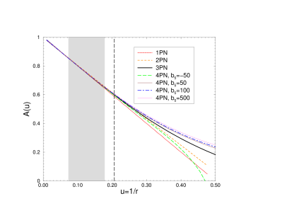
Figure 1: The potential $A(u)$ is plotted as a function $u=1/r\simeq GM/|{\bf x}_{1}-{\bf x}_{2}|$ at various PN orders. By varying the 4PN parameter $b_{5}$ we more than cover the behaviour of both the 2nd and 3rd post-Newtonian orders. In all the Figures, for a total mass $M=20M_{\odot}$, the gray-shaded region corresponds to the frequency band $[65,235]$ Hz, centered at 150 Hz, in which the signal-to-noise ratio accumulated for inspirals is more than 80% of the total SNR in the entire LIGO band. The corresponding range in $u$ is $0.07372\leq u\leq 0.1777$ and $r$ is $13.56\geq r\geq 5.63$. The dashed vertical line at $u_{\rm lso}=0.2065$ near the shaded region corresponds to the radial coordinate $r_{\rm lso}=4.84$ at which the system reaches the last stable circular orbit.

V.2 Unknown third post-Newtonian energy flux $\theta$

As mentioned in Sec. II the gravitational energy flux at third post-Newtonian order has one undetermined parameter $\theta$. We also argued in Sec. IV.3 that the magnitude of $\theta$ should be of order 1. Since the flux plays a crucial role in the phasing of the waves it is important to measure the effect of this parameter. In other words what fraction of the signal-to-noise ratio will be lost by setting $\theta=0$ in our templates while in reality $\theta$ is different from zero? Obviously, the answer depends on the extent by which $\theta$ is different from zero. We vary $\theta$ from $-5$ to $+10$ and plot the Newton-normalized flux as a function of the invariant velocity parameter $v$. As in Fig. 1 here too the shaded region corresponds to a frequency band $[65,235]$ Hz around 150 Hz corresponding to the range $0.2719\leq v\leq 0.4174$ when the total mass $M=20M_{\odot}$ (as assumed in Fig. 1). The dashed vertical line is of course the “velocity” at the last stable orbit $v_{\rm lso}=0.446$ corresponding to two systems of equal mass (independently of the value of the total mass).

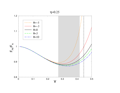
Figure 2: Variation in the (Newton-normalized) energy flux emitted by the system due to the 3PN parameter $\theta$ being different from zero. Clearly, negative values of $\theta$ have a greater effect on the behaviour of the flux as compared to the positive values.

Figure 2 indicates the extent of variation caused by changing the value of $\theta.$ Clearly, negative values of $\theta$ have a larger impact on the flux than positive values. Indeed, $\theta=-5$ leads to much greater variation in the flux than even $\theta=+10.$ The main message from Fig. 2 is that by varying $\theta$ over the range $-5\leq\theta\leq 10$ in our study of faithfulness and effectualness we would in effect take into account the possibility that the real gravitational wave flux be rather different from that assumed in the effective one-body approximation. (Note, however, that the differences within the most relevant shaded region are only $\sim\pm 10\%$.) The variation in $\theta$ we consider is far greater than the variation of $\pm 2$ in the parameter $\hat{\theta}$ considered in Ref. BCV02 . Note that $\hat{\theta}$ is related to our $\theta$ via

$$\hat{\theta}\equiv\theta+\frac{1987}{1320}\,.$$ (56)

Indeed our range corresponds to $-3.49\leq\hat{\theta}\leq 11.5$.

V.3 Flexibility parameter $c_{P}$

In Fig. 3 we plot the standard P-approximant flux at 3PN order in the equal mass case (i.e., $\eta=0.25$, solid line). In the notation introduced in Sec. IV.2 this curve corresponds to $c_{P}=0.$ The effect of changing the location of the pole is shown by plotting the energy flux for four values of the parameter $c_{P}$. We note that the curves change monotonically as the value of $c_{P}$ is changed, moving to the right for negative values of $c_{P}$ and to the left for positive values. We have changed the location of the pole by rougly 50% on either side of its nominal value. As mentioned before this amounts to varying the light ring value of $v$ in the range $0.4605\leq v_{\text{light ring}}\leq 1.3814$. No calculation we are aware of suggests a larger variation in the location of the pole than considered here. The curves do show a rather large variety indicating that the location of the pole is a priori as important as the other two parameters discussed before.

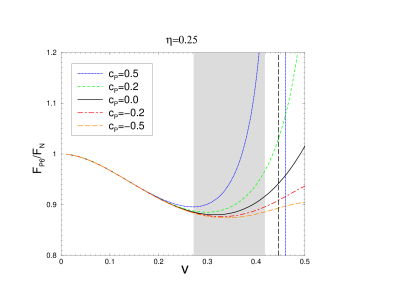
Figure 3: The (Newton-normalized) energy flux is plotted for different locations of the pole parametrised by $c_{P}.$ We vary the location of the pole by about 50% on either side of its nominal value predicted by the second post-Newtonian binding energy. The range of $c_{P}$ is perhaps far greater than what one could expect on physical grounds and causes a great variation in the flux function. Note that for $c_{P}=0.5$ the pole is moved to $v_{\rm pole}=0.4605$ which is near but still beyond the LSO.

VI The span of the 3PN EOB bank: Overlap of fiducial template with flexed waveform

VI.1 Faithfulness and effectualness

The ultimate tool for testing the robustness is of course the overlap of template waveforms with flexed waveforms. Given a fiducial template $T(t;p_{k})$ and a flexed signal $S(t;p_{l},\pi_{a})$ their overlap ${\cal O}$ is defined as

$${\cal O}(T,S)\equiv\frac{\langle T\,,\,S\rangle}{\sqrt{\langle T\,,\,T\rangle\langle S\,,\,S\rangle}}\,,$$ (57)

where the scalar product is defined as usual by the Wiener formula

$$\langle X,Y\rangle\equiv 2\int_{0}^{\infty}\frac{df}{S_{h}(f)}\left[\tilde{X}(f)\tilde{Y}^{*}(f)+\tilde{X}^{*}(f)\tilde{Y}(f)\right].$$ (58)

Here $\tilde{a}$ denotes the Fourier transform of function $a(t)$, that is, $\tilde{a}(f)=\int_{-\infty}^{\infty}a(t)\exp(-2\pi ift)dt,$ $a^{*}(f)$ denotes complex conjugation of $a(f)$ and $S_{h}(f)$ is the (one-sided) noise spectral density of the detector. In computing overlaps we use the initial LIGO noise spectral density of Ref. DIS3 given by:

$$S_{h}(f)=1.44\times 10^{-46}\left[\left(\frac{4.64f}{f_{k}}\right)^{-56}+\left(\frac{f}{f_{k}}\right)^{-4.52}+3.25+2\left(\frac{f}{f_{k}}\right)^{2}\right]{\rm Hz}^{-1}\,,$$ (59)

where $f_{k}=150$ Hz. Since the noise curve rises very steeply at low frequencies the lower limit of the integral in Eq. (58) does not have to be zero. It suffices to choose a lower limit of 40 Hz so as not to lose more than 1% of the overlap for binaries with total mass $M\simeq 50M_{\odot}.$

Faithfulness $\cal F$ is defined as the overlap maximized only over the extrinsic parameters of the template, which in our case are simply a reference time $t_{\rm ref}$ at which the template waveform reaches a certain frequency (say 40 Hz) and the phase $\phi_{\rm ref}$ of the signal at that time:

$${\cal F}=\max_{t_{\rm ref},\phi_{\rm ref}}|{\cal O}(T,S)|.$$ (60)

Effectualness $\cal E$ is defined as the overlap maximized over not only the extrinsic parameters but all the intrinsic parameters as well, which in our case are the two masses $m_{1}$ and $m_{2}$ of the binary:

$${\cal E}=\max_{t_{\rm ref},\phi_{\rm ref},m_{1},m_{2}}|{\cal O}(T,S)|.$$ (61)

VI.2 Matched filtering and signal-to-noise ratio

In searching for signals of known shape, such as chirping radiation from black hole binaries, one employs the method of matched filtering. For signals of known pattern, matched filtering is, in Gaussian noise background, a statistically optimum strategy in which a data analyst computes the cross-correlation of the template waveform $T(t)$ with the detector output $X(t).$ The analyst will not know before hand when the signal arrives or what its parameters are. Therefore, it is necessary to take several copies of the template corresponding to different parameter values $p_{k}$ and compute the correlation of each of those templates with the detector output at different time-steps $t_{0},t_{1},\ldots,t_{k},\ldots\,$. If detector output contains a sufficiently strong signal resembling one of the template waveforms then the cross-correlation will exceed the rms value of the correlation by a large amount, thereby generating a trigger for the analyst. It is well-known that the signal-to-noise ratio $\rho$ of a template $T$ with the detector output that contains a signal $S$ of known shape is given by

$$\rho\equiv\frac{s}{\overline{n}}=\frac{|\langle T,S\rangle|}{\langle T,T\rangle^{1/2}}=|{\cal O}(T,S)|\langle S,S\rangle^{1/2}.$$ (62)

Here $\langle S,S\rangle^{1/2}$ is the signal-to-noise ratio which would be achievable by matched filtering if the detector output were correlated with the exact replica of the signal hidden in the noise modulo the amplitude which is irrelevant. The above equation tells us that when we do not know the exact shape of the signal, the signal-to-noise ratio gets degraded and only a fraction equal to the overlap of the template used in the search with the exact signal expected to be present in the detector output is what is recoverable. Thus, while matched filtering is an excellent technique in detecting signals buried in noise, dephasing of the template relative to the signal can quickly degrade the quality of the output. This can be readily seen from Eq. (58) where the Fourier amplitudes of the template and the signal are multiplied together before being integrated over the frequency. These amplitudes coherently add up only when the phase of the template coincides with that of the signal at all points in the frequency space. Even a small initial difference in phase can accumulate and kill the integral since the signals last for a large number of cycles—more than 60 cycles for $(10M_{\odot}$,$10M_{\odot})$ black hole binaries and up to 1000 for NS-NS binaries in the sensitivity band of the LIGO interferometers. This is the motivation for building template waveforms that are as close to the true general relativistic signal as possible. Note, however, that the weighting of the overlap integral Eq. (58) by the inverse of the noise spectral density means that not all cycles in the signal and the template, are equally important. Ref. DIS2 introduced the concept of “useful cycles” as a measure of the effective number of cycles which dominate the overlap integral. For instance in the case of a $(10M_{\odot},10M_{\odot})$ system the number of useful cycles is $\simeq 7.6$. This means that it is crucial to model the phasing of the signal during the $\sim 8$ cycles around the peak of the SNR logarithmic frequency-distribution i.e. around $f_{P}\simeq 165$Hz, but that a less accurate model of phasing for the other cycles may be acceptable.

VI.3 Span of a template bank

Stringent as it may sound, matched filtering is not totally restrictive when dealing with a template bank rather than a single template. To explain how a template bank is not as restrictive as a single template we introduce the notion of span of a template bank. In the geometrical language of signal analysis BSD96 templates can be thought of as vectors—one vector for every set of values of the parameters $p_{k}.$ If the signal depends on $K$ parameters then the set of all vectors run over a $K$-dimensional manifold. Equation (58) serves as a scalar product between different vectors and induces a natural metric $g_{km}$ on the template-manifold with the parameters serving as natural coordinates:

$$g_{km}\equiv\langle T_{k}\,,T_{m}\rangle,\ \ T_{k}\equiv\frac{\partial T}{\partial p_{k}}.$$ (63)

Though each template is itself a vector in the vector space of all detector outputs, the set of all templates do not form a vector space. Therefore, when dealing with the problem of constructing a bank of templates one is really working with only a subspace of the vector space. Moreover, one does not work with the full template space either but, like in quantum mechanics, with the set of rays, i.e. the set of vectors modulo their lengths, which can be realized as the set of normalized vectors. In other words, we work on the unit sphere in the initial vector space. When considering a submanifold on this sphere which is not the intersection of a linear space with the unit sphere the metric $g_{km}$ gives only a local approximation to the vector product of the larger space, but it does not endow the finite-dimensional submanifold with the correct projection of the metric structure of the larger space.

In our search for gravitational-wave signals we choose a grid of templates on the template-manifold. If the templates are an exact replica of the expected signal then the density of the grid points is so chosen that no signal vector on the manifold has an overlap with the “nearest” grid point smaller than a certain fraction called the minimal match MM SD91 ; Owen96 , typically chosen to be either $\text{MM}=0.965$ or possibly $\text{MM}=0.95$:

$$\max_{\text{ Template bank}}|{\cal O}(T,S)|\geq\text{MM}.$$ (64)

Table 2: Robustness of 3PN EOB model with respect to parameters $b_{5}$, $\theta$, $\zeta_{2}$ and $c_{P}$. We give the faithfulness $\cal F$, effectualness $\cal E$, and the total mass $M^{\prime}$ and symmetric-mass ratio $\eta^{\prime}$ that maximize the overlap while finding effectualness. We vary each parameter in the nominal range but also quote extreme values of the parameters up to which an overlap of 95% or greater is obtained. Some parameters, for example $b_{5}$ will be bounded either from below or above since the physical quantity it participates in may be irregular for such values thereby affecting gravitational-wave phasing.

System $\rightarrow$	$(10M_{\odot},10M_{\odot})$			$(15M_{\odot},15M_{\odot})$
parameter $\downarrow$	${\cal F}$	${\cal E}$	$(M^{\prime},\eta^{\prime})$	${\cal F}$	${\cal E}$	$(M^{\prime},\eta^{\prime})$
$b_{5}=-50$	0.9754	0.9944	(20.25, 0.2479)	0.9728	0.9953	(30.41, 0.2494)
$b_{5}=+50$	0.9431	0.9850	(19.76, 0.2499)	0.9448	0.9943	(29.25, 0.2499)
$b_{5}=+190$	0.8566	0.9663	(19.61, 0.2500)	0.8855	0.9829	(28.92, 0.2500)
$b_{5}=+250$	0.8359	0.9633	(19.63, 0.2485)	0.8476	0.9766	(28.54, 0.2500)
$b_{5}=+300$	0.8014	0.9558	(19.48, 0.2500)	0.8363	0.9753	(28.46, 0.2500)
$b_{5}=+500$	0.7849	0.9498	(19.46, 0.2499)	0.8181	0.9694	(28.46, 0.2499)
$c_{P}=-0.2$	0.9988	0.9999	(19.97, 0.2500)	0.9993	0.9998	(29.96, 0.2500)
$c_{P}=+0.2$	0.9941	0.9989	(20.17, 0.2469)	0.9975	0.9999	(30.31, 0.2469)
$\theta=-5$	0.9358	0.9949	(20.27, 0.2500)	0.9642	0.9971	(30.77, 0.2497)
$\theta=+10$	0.9946	0.9982	(19.97, 0.2500)	0.9964	0.9999	(29.86, 0.2498)
$\zeta_{2}=-2$	0.9999	1.0000	(20.01, 0.2497)	0.9998	0.9998	(30.02, 0.2493)
$\zeta_{2}=+2$	0.9999	1.0000	(20.01, 0.2500)	0.9998	0.9999	(30.08, 0.2490)

The above inequality will be satisfied not only for signal vectors on the template manifold but also vectors that are off the manifold but close to it. In other words, the template bank obtains minimal match for all signals located in an infinite dimensional “slab” around the $K$-dimensional template manifold but sufficiently close to it. This “slab” defines the span of the considered template bank, say ${\cal S}[T,{\rm MM}]$. Here, for simplicity we introduce one flexibility parameter at a time and explore successively the “slab” along the directions defined by each extra parameter. It therefore suffices to consider only those signals that live in a $(K+1)$-dimensional space around the template manifold, which particular $K+1$, depending on the flexibility parameter in question. The span ${\cal S}[T,{{\rm MM}}]$ of a template bank along a given flexibility direction is then defined as the maximum domain in the corresponding $(K+1)$-dimensional space within which the template bank $T$ obtains a given minimal match MM. In this work we estimate this domain by computing the range of the flexibility parameters within which the minimal match is achieved between the fiducial template and flexed waveforms.

When the template is not a true representation of the signal, the signal vectors run over a manifold that does not exactly coincide with the template manifold. What is required for signal detection is that the span of the template bank includes the signal-manifold. Of course, if the minimal match is sufficiently small then any template bank would span the signal-manifold. Successful signal detection, without undue loss of signals, requires the signal-manifold to be a submanifold of ${\cal S}[T,0.95]$ (i.e., 95% minimal match) or, better, of ${\cal S}[T,0.965]$ (i.e., 96.5% minimal match).

Finally, let us note that while the span is defined with respect to a continuum of template bank in reality we will have to be content with a finite lattice of templates. Therefore, it is not guaranteed that the (maximum of the) overlap of a finite template bank with an arbitrary flexed signal within the span ${\cal S}[T,\ 0.965]$ will be greater than 0.965. If the template lattice is chosen such that the minimal match is at least 0.965 then the maximum overlap reached within the span ${\cal S}[T,\ 0.965]$ of the template bank might be reduced to $0.965^{2}\simeq 0.93.$ So the actual loss in the event rate might be $1-(0.965^{2})^{3}\simeq 20\%.$

VI.4 Span of third post-Newtonian EOB template bank

The main conclusion of this study is that the standard 3PN EOB template bank without any additional parameter, spans the extensions separately implied by the seven flexibility parameters that account for the unmodelled effects in the EOB formalism affecting both the dynamics and radiation flux. This is demonstrated in Tables 2 and 3 where we have considered two archetypal binaries expected to be observed by initial interferometers—the first consisting of a pair of $10M_{\odot}$ black holes and the second consisting of two $15M_{\odot}$ black holes. In Table 2 we have explored the faithfulness and effectualness of the 3PN EOB template bank (our fiducial template) with respect to the four important flexibility parameters $b_{5},$ $c_{P},$ $\theta$, and $\zeta_{2}$ and in Table 3 the same, but for the less important flexibility parameters $f_{\rm NonAdiab},$ $f_{\rm NonCirc},$ and $f_{\rm transition}.$

First, we discuss the results obtained by varying the parameters over the range in which they are expected to lie. Clearly, the 4PN parameter $b_{5}$ has the strongest influence followed by the parameters $c_{P},\theta$ and $\zeta_{2}.$ Indeed, the faithfulness is not always larger than the fiducial minimal match of 0.965 when these parameters take values over the range in which they are expected to vary. However, for $(15M_{\odot},15M_{\odot})$ systems the effectualness does easily meet the usual requirement ${\cal E}>0.965$ for all values of $b_{5}$ [including $b_{5}>500$, in view of the fact, visible on Fig. 1, that $A(u;b_{5})$ monotonically reaches a smooth limit as $b_{5}\rightarrow+\infty$]. In the case of $(10M_{\odot},10M_{\odot})$ systems the situation is a bit more involved: (1) when $b_{5}\lesssim 200$, the usual requirements on effectualness is met, but (2) when $b_{5}>200$, the effectualness drops slightly below $0.965$. However, for the “plausible” value $b_{5}=250$ (see Sec. IV above) the overlap is still larger than $0.963$, and even for $b_{5}=500$ (and probably for any larger $b_{5}$ for the reason mentioned above) the overlap is still as large as $0.95$. Note also that, in many cases, faithfulness is itself larger than the minimal match and effectualness is close to 1.

In view of this special sensitivity to $b_{5}$, we explored in detail the $b_{5}$-dependence of overlaps and found a simple modification of the standard 3PN EOB templates that allows for meeting the desired requirement ${\cal E}>0.965$ for all values of $b_{5}$. If one constructs a fiducial template bank by using as EOB potential the “$b_{5}$-flexed” function $A_{50}(u)\equiv A_{\text{4PN}}(u;b_{5}=50)$ [instead of $A_{\text{3PN}}(u)$], we have found that it leads to effectualness larger than 0.965 in all cases [and in particular for the $(10M_{\odot},10M_{\odot})$ system and $-50\leq b_{5}\leq 250$]. Furthermore, as illustrated in Table 4, the span of this new fiducial template bank now extends over all the values of $b_{5}$: $-50\leq b_{5}\leq 2000$. In the case of the less important parameters $f_{\rm NonAdiab},$ $f_{\rm NonCirc},$ and $f_{\rm transition},$ we observe that the faithfulness is itself larger than our minimal match except when $f_{\rm transition}=1$ for the $(15M_{\odot},15M_{\odot})$ system.

As mentioned in Sec. IV we have also explored robustness beyond the range in which the flexibility parameters are expected to lie and yet achieve the required effectualness. In Table 4 we summarize the range over which the different parameters are expected to vary together with the range over which they can be varied yet maintaining an effectualness of 0.965. This table shows that the span of the 3PN EOB bank of templates (or for that matter, the $b_{5}=50$-flexed 3PN one) in the other flexibility directions extend well beyond the expected plausible ranges.

VI.5 How could the match be good when the flux functions look so very different?

In Sec. V we noted that the behaviour of the energy flux $F_{P_{n}}(v)/F_{N}(v)$ could be significantly different from their usual behaviour when the flexibility parameters are set to extreme values in their expected range. When the flux is so different how is it still possible to achieve good effectualness?

The answer lies in several aspects of the problem: First, one should note that, after factorisation of the crucial “quadrupolar flux” $\propto v^{10}$, the changes in the Newton-normalized flux are less than $10\%$. Second, one should remember that for the massive binaries considered here, the number of “useful” gravitational-wave cycles DIS2 corresponding roughly to shaded regions in Figs. 2 and 3 is quite moderate ($\lesssim 8$). Third, one should note that one of the crucial things affected by the flux is the total chirp time, or the duration, of the waveform. For instance, if the flux increases more rapidly when one of the flexibility parameters is nonzero, as in the case of $\theta=-5,$ then the system loses energy more rapidly and therefore the waveform lasts shorter. However, this shortening of the waveform can also be achieved by making the binary heavier (or lengthened by making asymmetric binaries of the same total mass or simply lighter binaries). Recall that the effectualness is obtained by maximizing the overlap over both the extrinsic and intrinsic parameters. Thus, in the process of maximization one can absorb a change in time-scale by choosing a binary of different total mass and mass ratio. This explanation is borne out by a comparison of the trend of the curves in Figs. 1, 2 and 3 with the corresponding rows in Table 2. For instance, effectualness for $\theta>0$ (smaller flux at a given $v$ than when $\theta=0$) requires a system of total mass lighter than the original system while for $c_{P}>0$ (greater flux at a given $v$ than when $c_{P}=0$) one requires a heavier system than the original one.

A final comment: The insensitivity of the effectualness to the location of the pole can be interpreted to mean that the factorisation by the pole is not as crucial an element of the gravitational-wave flux resummation as perceived in DIS1 . This suggests that it would be interesting to study the performance of templates which do not use such a factorisation of the flux function. We leave this study to future work.

Table 3: Robustness of 3PN EOB model with respect to parameters ${f}_{\rm NonAdiab}$, ${f}_{\rm NonCirc}$, and ${f}_{\rm transition}$. We give the faithfulness $\cal F$, effectualness $\cal E$, and the total mass $M^{\prime}$ and symmetric-mass ratio $\eta^{\prime}$ that maximize the overlap while finding effectualness. We vary each parameter in the nominal range but also quote extreme values of the parameters up to which an overlap of 95% or greater is obtained.

System $\rightarrow$	$(10M_{\odot},10M_{\odot})$			$(15M_{\odot},15M_{\odot})$
Parameter $\downarrow$	${\cal F}$	${\cal E}$	$(M^{\prime},\eta^{\prime})$	${\cal F}$	${\cal E}$	$(M^{\prime},\eta^{\prime})$
${f}_{\rm NonAdiab}=-1.0$	0.9976	1.0000	(20.04, 0.2491)	0.9967	1.0000	(30.11, 0.2486)
${f}_{\rm NonAdiab}=+1.0$	0.9979	0.9999	(20.00, 0.2500)	0.9964	0.9999	(30.01, 0.2496)
${f}_{\rm NonCirc}=-1.0$	0.9998	0.9998	(20.09, 0.2473)	0.9997	0.9999	(30.02, 0.2500)
${f}_{\rm NonCirc}=+1.0$	0.9998	0.9999	(20.10, 0.2472)	0.9996	1.0000	(30.04, 0.2500)
${f}_{\rm transition}=0.5$	1.0000	1.0000	(20.00, 0.2500)	0.9967	0.9994	(30.03, 0.2498)
${f}_{\rm transition}=1.0$	0.9877	0.9878	(20.01, 0.2500)	0.9531	0.9606	(30.26, 0.2498)

VI.6 Systematic versus statistical errors in the estimation of parameters

Together with the value of the effectualness, the tables also show the template parameters that obtain the maximized overlaps. A quick inspection reveals that the symmetric mass ratio $\eta$ of the template that obtained the maximum match is either equal to the actual value of 1/4 or when different from 1/4 the fractional difference is less than 0.1%. This is probably explained by the following: We study templates as functions of $m_{1}$ and $m_{2}$. But the function $T(m_{1},m_{2})$ is invariant under the permutation $m_{1}\leftrightarrow m_{2}$ and therefore the overlap ${\cal O}(m_{1},m_{2})=\langle T(m_{1},m_{2}),S\rangle$ always reaches an extremum (along the lines $m_{1}+m_{2}=\text{constant}$) at $m_{1}=m_{2}$, i.e. at $\eta=1/4$. If these extrema are all maxima (as a function of the ratio $m_{1}/m_{2}$, for a fixed value of $m_{1}+m_{2}$), the real maximum of the overlap must lie somewhere along the “ridge” $m_{1}=m_{2}$. Note, however, that there might as well be domains of parameter space where the overlap ${\cal O}(m_{1},m_{2})$ reaches a minimum along the ridge at $m_{1}=m_{2}$ (at fixed mass scale $m_{1}+m_{2}=\text{constant}$). The total mass is different from the true total mass at worst by about 1.5%. These percentages, of course, do not give us a measure of the accuracy of estimation of the parameters, rather they tell us the extent of bias induced in the estimation. Since our template bank contains waveforms that are not exactly the same as the “true” signals, the parameters that maximize the overlap are different from the real values meaning there is a systematic error in the estimation of parameters and the percentages we have quoted are upper limits on the systematics.

The statistical errors in the estimation of the intrinsic parameters $m_{1},m_{2}$ are determined by the shape of the level contours of the overlap function between the template $T(m_{1},m_{2})$ and the signal, that we assume here to be part of the template bank: $S=T(m^{0}_{1},m^{0}_{2})$. For high signal-to-noise ratio this shape is an ellipse (the error ellipse) which is determined by the information matrix, i.e.  the metric Eq. (63). We have confirmed that even for the massive binary systems that we consider, these error contours are qualitatively well described by the analytical results of PoissonAndWill , i.e.  that, when represented in the $({\cal M},\eta)$-plane, where ${\cal M}=\eta^{3/5}M$ is the chirp mass, they are highly elongated ellipses with major axis roughly along the $\eta$-direction and minor axis along the ${\cal M}$-direction. When represented in the $(m_{1},m_{2})$-plane these error contours have the shape of thin crescents orthogonal to the diagonal $m_{1}=m_{2}$. A bad consequence of this fact is that there can be a large statistical error in the determination of $\eta$ PoissonAndWill , and therefore correspondingly large statistical errors in the determination of the individual masses. Only the combination ${\cal M}=\eta^{3/5}M$ might be reasonably free of statistical errors. A more detailed analysis is needed to assess the total errors combining systematic and statistical effects.

We note in passing that a useful consequence of the highly elongated structure of the overlap contours is to allow a fast first-cut data analysis based on the lower-dimensional template bank defined by fixing $\eta$, e.g. to $1/4$, and varying only $M=m_{1}+m_{2}$. The choice $\eta=1/4$ would be sufficient to cover systems in a large domain of mass space around the diagonal $m_{1}=m_{2}$. It can then be complemented by considering a few other simple values of $\eta$. Each such lower-dimensional (approximate) template bank (corresponding to some value of $\eta$) finally depends on only one universal function of one variable, the scaled phasing function $\phi_{\eta}(\hat{t})$, obtained by integrating, once for all, the EOB equations of motion expressed in terms of scaled variables $\hat{t}=t/M,\,r\simeq|{\bf x}_{1}-{\bf x}_{2}|/GM$, for a particular $\eta,$ extending to EOB the idea of mother templates for the post-Newtonian model BSS00 . The bank of templates is then built from the shifted and scaled function $\phi_{\eta}((t-t_{0})/M)$. This fact should simplify further the filter bank construction similar to the case of Newtonian signals which were expressible in terms of the universal function $\phi_{N}(\hat{t})\propto-(-\hat{t})^{5/8}$. Indeed, the fact that this must be so is implicit in the nature of the template bank constructed by several authors (cf. second reference in Owen96 and Ref.BSS94 ) who find that a small range of $\eta$ is needed for a large range of the total mass.

Table 4: The natural range for the flexibility parameters expected on physical grounds is shown together with the actual span for which the effectualness is greater than 0.965 for equal mass binaries of total mass 20$M_{\odot}$ and $30M_{\odot}$. As discussed in the text the span in the $b_{5}$-direction refers to a bank of templates constructed with slightly modified EOB potential: $A_{50}(u)$.

Range/Span	$b_{5}$	$c_{P}$	$\theta$	$\zeta_{2}$	$f_{\rm NonAdiab}$	$f_{\rm NonCirc}$	$f_{\rm transition}$
Expected Range	$[0,250]$	$[-0.2,0.2]$	$[-5,10]$	$[-2,2]$	$[-1,1]$	$[-1,1]$	$[0,0.5]$
Span ${\cal S}(T,0.965)$	$[-50,2000]^{\*}$	$[-0.5,0.5]$	$[-5,>\!\!1000]$	$[-5,100]$	$[-20,15]$	$[-50,50]$	$[0,1]$

VII Conclusions

In this study we have explored the robustness of 3PN EOB templates. We introduced seven flexibility parameters that affect the two-body dynamics and radiation emission and varied each of them separately over a range that can be reasonably considered to be large enough to encompass unknown and unmodelled PN effects. The parameters introduced are: (a) a 4PN parameter $b_{5}$ that alters the two-body effective metric and the EOB potential $A(u)$. We conducted a special study of the structure of 4PN contributions to the Hamiltonian to estimate the plausible range of the parameter $b_{5}$ measuring them ($-50\leq{b_{5}}\leq 250$). (b) the unknown 3PN parameter $\theta$ affecting the nature of the energy flux emitted by the system ($-5\leq\theta\leq 10$). (c) a parameter $\zeta_{2}$ that changes ${\cal O}({\bf p}^{2}p_{r}^{2})$ terms in the two-body Hamiltonian ($-2\leq{\zeta_{2}}\leq+2$). (d) location of the pole in the energy flux controlled by a parameter $c_{P}$. (e) and three parameters $f_{\rm NonAdiab}$, $f_{\rm NonCirc}$, and $f_{\rm transition}$, that are varied so as to inflict at least a factor two change in the modelling of non-adiabatic effects, non-circular effects and the transition from inspiral to plunge, respectively.

We then compared the faithfulness and effectualness of standard fiducial EOB templates (that is, EOB templates in which all the above parameters are set equal to zero) with the flexed signals obtained by switching on the flexibility parameters one at a time. Based on the study conducted in this work we find that the third post-Newtonian EOB templates lead to effectualness larger than 96.3% in all cases (when $b_{5}\leq 250$). For the $(10M_{\odot},10M_{\odot})$ systems, and $b_{5}$ larger than 190 the effectualness drops below the usual requirement ${\cal E}>0.965$, though it remains very close to it, being larger than 0.96. (Even when $b_{5}$ gets very large the effectualness never drops below 0.95.)

There are two ways of improving this situation linked to the special sensitivity to $b_{5}$. One way is to augument the standard 3PN bank of templates [based on $A_{\text{3PN}}(u)$] by (when it is needed) a second bank of templates, based on $A_{100}(u)\equiv A_{\text{4PN}}(u;b_{5}=100)$. We have checked that this “doubled” bank of templates allows one to span all values of $b_{5}$ with overlaps better than 0.985. A second way (which minimizes the total number of templates needed) is to work in all cases with only one specific $b_{5}$-flexed bank of templates [namely the one based on the “intermediate” EOB potential $A_{50}(u)\equiv A_{\text{4PN}}(u;b_{5}=50)$]. The remarkable agreement between numerical and analytical descriptions of circular orbits near the LSO DGG02 ; B02a , suggests that it might be possible soon to use numerical simulations to map in detail the EOB potential $A(u)$ near the LSO. Hopefully this might lead to a numerical estimate of the value of $b_{5}$ thereby sharpening the preferred choice of bank of templates.

There is a caveat in the current evaluation which we must bear in mind namely that we vary the flexibility parameters only one at a time. It is possible that the actual physical signal has more than one of the flexibility parameters non-zero. In that case our fiducial templates might not be able to achieve the desired span. This is because the ‘shifts’ in the fiducial template parameters needed to separately correct for the various non-zero flexibility parameters might be in different ‘directions’. An attempt to define a rather phenomenological signal was the main focus of Ref. BCV02 . In this paper, we have focussed on a different (minimalistic) attitude and have not looked into these matters. We intend to address this issue in a future work.

To conclude: the 3PN EOB templates (possibly suitably $b_{5}$-flexed) are good models to use for black hole binary searches in the interferometer gravitational-wave data because their “span” in signal space seems large enough to encompass most of the plausible modifications one can think of making in the current EOB framework. Moreover, as we emphasized, the highly elongated shape of overlap contours in the $(M,\eta)$-plane suggests the interesting possibility to drastically reduce the number of EOB templates by using a small number of universal phasing functions $\phi_{{\eta}_{i}}(\hat{t})$ with a small discrete set of values of $\eta$ prominently including $\eta=1/4$.

- (1) L. P. Grishchuk, V. M. Lipunov, K. A. Postnov, M. E. Prokhorov, and B. S. Sathyaprakash, Phys. Usp. 44, 1 (2001); Usp. Fiz. Nauk 171, 3 (2001).
- (2) A. Buonanno, Y. Chen, and M. Vallisneri, Detection template families for gravitational waves from the final stages of binary-black-hole inspirals. I. Nonspinning case, Phys. Rev. D (2002) (To Appear); gr-qc/0205122.
- (3) A. Buonanno and T. Damour, Phys. Rev. D 59, 084006 (1999).
- (4) A. Buonanno and T. Damour, Phys. Rev. D 62, 064015 (2000).
- (5) T. Damour, P. Jaranowski, and G. Schäfer, Phys. Rev. D 62, 084011 (2000).
- (6) T. Damour, Phys. Rev. D 64, 124013 (2002).
- (7) T. Damour, B. R. Iyer, and B. S. Sathyaprakash, Phys. Rev. D 63, 044023 (2001).
- (8) E. Gourgoulhon, P. Grandclément, S. Bonazzola, Phys. Rev. D 65, 044020 (2002); P. Grandclément, E. Gourgoulhon, S. Bonazzola, Phys. Rev. D 65, 044021 (2002).
- (9) T. Damour, E. Gourgoulhon, and P. Grandclément, Phys. Rev. D 66, 024007 (2002).
- (10) L. Blanchet, Phys. Rev. D 65, 124009 (2002).
- (11) T. Damour, B. R. Iyer, and B. S. Sathyaprakash, Phys. Rev. D 57, 885 (1998).
- (12) C. Cutler et al., Phys. Rev. Lett. 70, 2984 (1993).
- (13) P. Jaranowski and G. Schäfer, Phys. Rev. D 57, 7274 (1998); 60, 124003 (1999).
- (14) T. Damour, P. Jaranowski, and G. Schäfer, Phys. Rev. D 62, 044024 (2000); 62, 021501(R) (2000) [Erratum: 63, 029903(E) (2001)]; 63, 044021 (2001).
- (15) L. Blanchet and G. Faye, Phys. Lett. A 271, 58 (2000); Phys. Rev. D 63, 062005 (2000).
- (16) L. Blanchet and G. Faye, J. Math. Phys. 41, 7675 (2000); 42, 4391 (2001).
- (17) V. C. de Andrade, L. Blanchet, and G. Faye, Class. Quantum Grav. 18, 753 (2001).
- (18) L. Blanchet and B. R. Iyer, Class. Quantum Grav. 20, 755 (2003)
- (19) T. Damour, P. Jaranowski, and G. Schäfer, Phys. Lett. B 513, 147 (2001).
- (20) L. Blanchet and T. Damour, Phil. Trans. R. Soc. London A 320, 379 (1986); L. Blanchet, Proc. R. Soc. Lond. A 409, 383 (1987); L. Blanchet and T. Damour, Phys. Rev. D 37, 1410 (1988); Ann. Inst. H. Poincaré (Phys. Théorique) 50, 377 (1989); T. Damour and B. R. Iyer, Ann. Inst. H. Poincaré (Phys. Théorique) 54, 115 (1991); Phys. Rev. D 43, 3259 (1991); L. Blanchet and T. Damour, Phys. Rev. D 46, 4304 (1992); L. Blanchet, Class. Quantum Grav. 15, 1971 (1998).
- (21) L. Blanchet, T. Damour, B. R. Iyer, C. M. Will, and A. G. Wiseman, Phys. Rev. Lett. 74, 3515 (1995); L. Blanchet, T. Damour, and B. R. Iyer, Phys. Rev. D 51, 5360 (1995); C. M. Will and A. G. Wiseman, Phys. Rev. D 54, 4813 (1996); L. Blanchet, B. R. Iyer, C. M. Will, and A. G. Wiseman, Class. Quantum Grav. 13, 575, (1996); L. Blanchet, Phys. Rev. D 54, 1417 (1996).
- (22) L. Blanchet, Class. Quantum Grav. 15, 113 (1998).
- (23) L. Blanchet, G. Faye, B. R. Iyer, and B. Joguet, Phys. Rev. D 65, 061501(R) (2002).
- (24) L. Blanchet, B. R. Iyer, and B. Joguet, Phys. Rev. D 65, 064005 (2002).
- (25) T. Damour, B. R. Iyer, and B. S. Sathyaprakash, Phys. Rev. D 66, 027502 (2002).
- (26) L. Blanchet, in Proceedings of the 25th Johns Hopkins Workshop, Eds. I. Ciufolini and L. Lusanna; gr-qc/0207037.
- (27) L. Blanchet and B. R. Iyer, work in progress.
- (28) R. Balasubramanian, B. S. Sathyaprakash, and S. V. Dhurandhar, Phys. Rev. D 53, 3033 (1996).
- (29) B. S. Sathyaprakash and S. V. Dhurandhar, Phys. Rev. D 44, 3819 (1991).
- (30) B. J. Owen, Phys. Rev. D 53, 6749 (1996); B. J. Owen and B. S. Sathyaprakash, Phys. Rev. D 60, 022002 (1999).
- (31) T. Damour, B. R. Iyer, and B. S. Sathyaprakash, Phys. Rev. D 62, 084036 (2000).
- (32) E. Poisson and C. M. Will, Phys. Rev. D 52, 848 (1995).
- (33) B. S. Sathyaprakash, Class. Quant. Grav. 17, L157 (2000).
- (34) B. S. Sathyaprakash, Phys. Rev. D 50, R7111 (1994).