Alberta–Thy 17-02
Capture and Critical Scattering of a Long Cosmic String by a Rotating Black Hole

Abstract

The capture of a straight, infinitely long cosmic string by a rotating black hole with rotation parameter $a$ is considered. We assume that a string is moving with velocity $v$ and that initially the string is parallel to the axis of rotation of the black hole and has the impact parameter $b$. The string can be either scattered or captured by the black hole. We demonstrate that there exists a critical value of the impact parameter $b_{c}(v,a)$ which separates these two regimes. Using numerical simulations we obtain the critical impact parameter curve for different values of the rotation parameter $a$. We show that for the prograde motion of the string this curve lies below the curve for the retrograde motion. Moreover, for ultrarelativistic strings moving in the prograde direction and nearly extremal black holes the critical impact parameter curve is found to be a multiply valued function of $v$. We obtain real time profiles of the scattered strings in the regime close to the critical. We also study critical scattering and capture of strings by the rotating black hole in the relativistic and ultrarelativistic regime and especially such relativistic effects as coil formation and wrapping effect.

¹Theoretical Physics Institute, Department of Physics,  University of Alberta,
Edmonton, Canada T6G 2J1

1 Introduction

Cosmic strings are topologically stable one-dimensional objects which are predicted by unified theories and can be created during a phase transition in the early Universe [1]. Recent measurements of CMB anisotropy gave certain restrictions on the models of cosmic string formation but do not exclude their existence. The analysis shows that a mixture of inflation and topological defects is consistent with current CMB data [2, 3, 4, 5, 6].

When a cosmic string in its motion passes close to a black hole it can be captured. In this paper we study this phenomenon. We consider the string to be a test object moving in the background gravitational field of a rotating black hole. Test string approximation can be justified since the dimensionless parameter $\mu^{*}=G\mu/c^{2}$ ($\mu$ is the string mass per a unit length) is very small. For GUT energy strings $\mu_{GUT}^{*}\sim 10^{-6}$ and for EW energy scale $\mu^{*}_{EW}\sim 10^{-34}$. The emission of gravitational waves by the string, which might be of astrophysical interest, affects the string motion only in the order $\sim{\mu^{*}}^{2}$. This effect can be considered by using the perturbation methods. But first one must solve the equations of motion for the test string. This problem by itself is quite complicated because the equations are non-linear. If a string remains far from the black hole, one can linearize the string equations of motion. The solution of the linearized equations in the black hole spacetime was obtained and studied in [8, 9, 10, 11]. For the scattering at smaller impact parameters, and especially for the string capture non-linear effects are very important and the problem is to be treated numerically. The string scattering and capture by a non-rotating black hole was studied in [12, 13]. One might expect that in the most of the astrophysically interesting cases (such as a stellar mass black hole in a binary system or massive and supermassive black holes in the center of galaxies and quasars) the black hole is rotating or even to be close to extremally rotating. String scattering by a rotating black hole (including the non-linear regime) was discussed in our previous paper [11]. We demonstrated that as a result of scattering of an initially infinitely long straight string moving with velocity $v$ and an impact parameter $b$ the string, after passing the black hole, keeps moving with the same velocity, while the central part of the string moves in a new plane with a different impact parameter. The region of this ‘new phase’ expands as the kink-like transition layers connecting the ‘new’ and ‘old’ phases propagate with the velocity of light away from the center of the string. We studied the string scattering data, i.e., the change of the impact parameter and the width of the transition layers as a function of $v$ and $b$. We showed that for large $b$ the effects of the rotation are negligibly small and one can use a weak field approximation in this regime. For strings coming closer to the black hole the effect of rotation becomes more profound. We used numerical simulations to obtain the string scattering data in different regimes of scattering and the real time profiles of the strings.

In this paper we continue studying an interaction of a long cosmic string with a rotating black hole. Now we focus our attention on the capture and scattering in the special regime close to the capture. We consider a black hole of mass $M$ and angular momentum $J=aM$. We assume that initially a straight infinitely long cosmic string is parallel to the axis of rotation of the black hole, and it is moving with velocity $v$ and impact parameter $b$. For a rotating black hole we distinguish two principal type of motion. If the angular momentum of the black hole coincides with the direction of the angular momentum of the string the motion is called a prograde motion. In the opposite case it is called a retrograde motion. The initial setup of the cosmic string is schematically shown on figure 1. For large impact parameters, $b\gg M$, the string after coming to the black hole moves further and escapes to infinity. The capture occurs when the central part of the string comes close to the black hole and eventually crosses the event horizon. By central part we will always understand the part of the string close to the $Z=0$ symmetry plane.

For a given velocity $v$ there exist a critical value of the impact parameter, $b_{c}(v,a)$, which separates capture and scattering regimes. As we shall show, scattering of the string with the impact parameter slightly greater than $b_{c}(v,a)$ has a number of interesting features. We call this regime critical scattering. The second aim of this paper is to study this regime.

The paper is organized as follows. We remind the string equation of motion in section 2. In this section we also discuss the initial data for our problem. String capture and critical impact parameter curves are discussed in section 3. In section 4 for we present the real time profiles for critical string scattering and discuss the form of these profiles at the late time regime. The effect of coil formation for the relativistic strings is considered in section 5. In this section we present the results of the numerical simulations for the coil formation regions and compare them with an analytical solution for the weak field scattering. The last section 6 contains general discussion and further remarks.

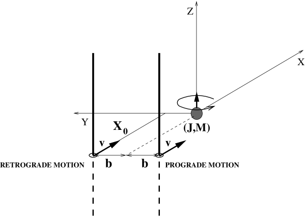
Figure 1: Initial setup for prograde and retrograde string motion. The part of the string depicted by the dashed line lies below the $X$-$Y$ plane.

2 String equation of motion

We consider long string motion in the Kerr spacetime with metric

$$ds^{2}=-(1-\frac{2Mr}{\Sigma})d\tilde{v}^{2}+2d\tilde{v}dr-\frac{4aMr\sin^{2}{\theta}}{\Sigma}d\tilde{v}d\tilde{\phi}-a\sin^{2}{\theta}drd\tilde{\phi}$$

$$+\Sigma d\theta^{2}+\frac{A\sin^{2}{\theta}}{\Sigma}d\tilde{\phi}^{2}\,.$$ (2.1)

Here

$$\Sigma=r^{2}+a^{2}\cos^{2}{\theta}\,,\hskip 14.22636pt\Delta=r^{2}-2Mr+a^{2}\,,$$

$$A=(r^{2}+a^{2})^{2}-a^{2}\Delta^{2}\sin^{2}{\theta}\ .$$ (2.2)

We use the so called Kerr (in-going) coordinates $(\tilde{v},r,\theta,\tilde{\phi})$ which are related to the standard Boyer-Lindquist coordinates $(t,r,\theta,\phi)$ as follows

$$\tilde{v}=t+r+M\ln|{\Delta\over 4M^{2}}|+\frac{M^{2}}{\sqrt{M^{2}-a^{2}}}\ln\left|\frac{r-M-\sqrt{M^{2}-a^{2}}}{r-M+\sqrt{M^{2}-a^{2}}}\right|+M\,,$$

$$\tilde{\phi}=\phi+\frac{a}{2\sqrt{M^{2}-a^{2}}}\ln\left|\frac{r-M-\sqrt{M^{2}-a^{2}}}{r-M+\sqrt{M^{2}-a^{2}}}\right|\ .$$ (2.3)

The string worldsheet $X(\zeta^{A})$ ($\zeta^{A}$, $A=0,1$) obeys the following equations

$$\Box{\cal X}^{\mu}+h^{AB}\Gamma^{\mu}_{\alpha\beta}{\cal X}^{\alpha}_{,A}{\cal X}^{\beta}_{,B}=0\,,$$ (2.4)

$$\gamma_{AB}-{1\over 2}h_{AB}h^{CD}\gamma_{CD}=0\,,$$ (2.5)

where

$$\Box={1\over\sqrt{-h}}\partial_{A}(\sqrt{-h}h^{AB}\partial_{B})\,.$$ (2.6)

The first of these equations is the dynamical equation for string motion, while the second one plays the role of constraints. These equations provide an extremum to the Nambu-Goto action (taken in the Polyakov form)

$$I[{\cal X}^{\mu},h_{AB}]=-{\mu\over 2}\,\int d^{2}\zeta\sqrt{-h}h^{AB}\gamma_{AB}\,.$$ (2.7)

We use units in which $G=c=1$, and the sign conventions of [14]. In (2.7) $h_{AB}$ is the auxiliary metric with determinant $h$.

We fix internal coordinate freedom by using the gauge in which $h_{AB}$ is conformal to the flat two-dimensional metric $\eta_{AB}=\mbox{diag}(-1,1)$. In this gauge the equations of motion for the string have the form

$$\Box_{0}{\cal X}^{\mu}+\Gamma^{\mu}_{\alpha\beta}\,{\cal X}^{\alpha}_{,A}\,{\cal X}^{\beta}_{,B}\,\eta^{AB}\,=0\,,$$ (2.8)

and the constraints are

$$\gamma_{01}=g_{\mu\nu}\frac{\partial{\cal X}^{\mu}}{\partial\tau}\frac{\partial{\cal X}^{\nu}}{\partial\sigma}=0\ ,$$ (2.9)

$$\gamma_{00}+\gamma_{11}=g_{\mu\nu}\left(\frac{\partial{\cal X}^{\mu}}{\partial\tau}\frac{\partial{\cal X}^{\nu}}{\partial\tau}+\frac{\partial{\cal X}^{\mu}}{\partial\sigma}\frac{\partial{\cal X}^{\nu}}{\partial\sigma}\right)\ =0\ .$$ (2.10)

Here, $\tau\equiv\zeta^{0}$, $\sigma\equiv\zeta^{1}$ and $\Box_{0}=-\partial^{2}_{\tau}+\partial^{2}_{\sigma}$.

It is easy to check that a solution for a straight string moving in a flat spacetime can be written as follows

$${\cal X}^{\mu}={\cal X}_{0}^{\mu}(\tau,\sigma)\equiv(\tau\cosh\beta,\tau\sinh\beta+X_{0},b,\sigma)\,,$$ (2.11)

$$h_{AB}=\eta_{AB}\equiv\mbox{diag}(-1,1)\,.$$ (2.12)

This solution describes a straight string oriented along the $Z$-axis which moves in the $X$-direction with constant velocity $v=\tanh\beta$. Initially, at ${\tau}_{0}=0$, the string is found at ${\cal X}^{\mu}(0,\sigma)=(0,X_{0},b,\sigma)$. We call $b$ an impact parameter. In our simulations we choose $b$ to be positive and $X_{0}$ to be large and negative.

To study string scattering and capture by the black hole we use numerical simulation. The general scheme is described in details in [11]. However, the simulation of critical scattering is computationally more involved and the adaptive mesh refinement algorithm has been improved. In our simulation we alter the grid density according to a truncation error estimate. If the error estimate in certain region of the grid lies above a prescribed threshold the calculation is restarted from a last stored state with the grid in the region (and its neighborhood) appropriately refined. Similarly, if the truncation error in some region of the grid is much smaller than the threshold the grid in that region is coarsened (this time, of course, it is not necessary to restart the calculation).

Here we just make some general remarks concerning the calculations. We assume that initially the string is very far away from the black hole where the spacetime is practically flat. We use the solution (2.11)) in this region. When the string comes closer to the black hole the gravitational field of the latter modifies its motion. When the distance $r$ from the black hole is much larger than the gravitational radius, $r>>M$, the gravitational field is still weak. One can linearize the string equations and obtain linear equations describing the string motion. It is possible to show (see [11]) that in this regime the effects connected with the rotation of the black hole can be neglected with respect to the Newtonian corrections. By solving the weak field equations one determines the string evolution in the weak field region. This solution is used to obtain initial data for numerical simulations. It also can be used to get the boundary conditions at “numerical ends” of the string. During the simulations the dynamical equations are numerically solved while the constraint equations are used as an additional check of the accuracy of the calculations.

3 String capture and critical impact parameter

Two outcomes are possible for the string evolution—scattering and capture. Capture occurs when a part of the string enters the event horizon of the black hole located at

$$r=M+\sqrt{M^{2}-a^{2}}\,.$$ (3.1)

Since the Kerr in-going coordinates are regular at the event horizon we can trace the string evolution both in the black hole exterior and interior. For our study of the string capture we stop our calculations as soon as part of the string crosses the horizon. The value of $b_{c}(v,a)$ is determined as follows. For each fixed velocity $v$ and angular momentum $a$ we start the search with two values of $b$—one for which the string is captured and one for which it escapes. Then we use bisection method to bracket the critical impact parameter. The results of these calculations are presented at figure 2. The error bars are smaller than the data markers so they are not shown.

Figure 2: Critical impact parameter $b_{c}$ as a function of the string’s initial velocity $v$

This plot contains the critical impact parameter curves for 9 different values of the rotation parameter $a$ from $a=-M$ to $a=M$. The signs are chosen so that a negative value of $a$ corresponds to a retrograde motion of the string and positive value to a prograde one. The lower the value of $a$ the higher is the position of the critical impact parameter curves in the $(v,b_{c})$–plane. This feature is easily explained by the dragging into rotation effect. Indeed, for the retrograde motion the dragging effect slows down the string’s motion. The string spends more time in the strong attractive field of the black hole and hence it can be captured easier. In order to escape the capture the string must be moving with larger impact parameter. Thus the critical impact parameter is larger that for a non-rotating black hole. For the prograde motion the effect is opposite.

Numerical calculations were done for $v/c>0.12$. For smaller velocity the impact parameter becomes large and computational time grows. On the other hand, for large impact parameters the main part of the time evolution of the string occurs in the weak field region. One can use this to estimate the critical impact parameter for low velocity motion. It was done by Don Page [9]. He proposed the following approximation for the critical impact parameter

$$b_{c}/M=\left(\sqrt{\frac{\pi}{2v}}-\sqrt{\frac{\pi}{2}}\right)-\frac{64}{15}\,(1-v)+3\sqrt{3}\,.$$ (3.2)

This function is shown in figure 2 by a solid line. One can see that it gives quite good approximation for a non-rotating black hole. For rotating black holes this line gives good approximation for small $v$ since for large impact parameters the rotation plays less important role.

It is instructive to compare the string scattering with the scattering of particles. In particular, in the ultrarelativistic limit $v/c\to\infty$ the critical impact parameter for the string coincides with the critical impact parameter for photons. The only exception is a case of prograde scattering by a nearly extreme black hole. Complicated structure of the critical impact parameter curve for this case is connected with the features of the near critical scattering which we discuss later. The capture parameter for particles in the the ultrarelativistic limit is (see e.g. [15])

$$b^{part}_{c}/M=8\cos^{3}\left[\frac{1}{3}(\pi-\arccos a)\right]+a\,.$$ (3.3)

The value of $b^{part}_{c}$ for $a/M=0,\pm 0.25,\pm 0.5,\pm 0.75,\pm 1$ is shown by stars on figure 2 on the vertical line at $v/c=1$. These points are very close to those belonging to an ultrarelativistic string. The only exception is a region of $a/M$ close to 1.

Figure 3: Critical impact parameter $b_{c}$ and its fitted approximation $b^{fit}_{c}$ as functions of the string’s initial velocity $v$ for different values of the rotation parameter $a/M$.

The Page’s approximation for critical impact parameter curves can be generalized to the case of a rotating black hole. We can write the corresponding ansatz in the form

$$b^{fit}_{c}/M=\left(\sqrt{\frac{\pi}{2v}}-\sqrt{\frac{\pi}{2}}\right)-(b_{0}+b_{1}\,a+b_{2}\,a^{2})\,(1-v)+b^{part}_{c}/M\,.$$ (3.4)

The best fit for numerically calculated critical impact parameter curves gives the following values of the fitting parameters $b_{i}$

$$b_{0}=4.40\,,\hskip 28.45274ptb_{1}=-1.55\,,\hskip 28.45274ptb_{2}=-0.53\,.$$ (3.5)

Figure 3 shows the result of the fitting for different values of $a/M=0,\pm 0.25,\pm 0.5,\pm 0.75,-1$. (We exclude $a/M=1$ because of the peculiar behavior of the critical impact parameter curve for this case.) It is easy to see that continuous curves representing $b^{fit}_{c}$ given by (3.4)–(3.5) are in a good agreement with the numerical data shown by shaped points.

Figure 4: Capture curve for a prograde scattering of a relativistic cosmic string by a rapidly rotating black hole.

Let us discuss an additional new feature in the critical impact curves which occurs for highly relativistic prograde scattering by rapidly rotating black holes. Plot for $a/M=1.0$ presented in figure 2 shows that in this regime $b_{c}(v,a)$ becomes a multiply valued function of $v$. We studied numerically this regime. Figure 4 shows the corresponding region in more details. It contains plots of $b_{c}(v,a)$ near $v/c=1$ for two values of the rotation parameter—$a/M=0.9$ and $a/M=1.0$. Besides the main branch curve (marked by ‘$+$’ for $a/M=0.9$ and by ‘$\circ$’ for $a/M=1.0$) there also exists an additional branch (marked by ‘$\ast$’ for $a/M=0.9$ and by ‘$\times$’ for $a/M=1.0$). We performed calculations up to $v/c=0.9995$ which corresponds to the gamma-factor $\gamma\approx 30$. For greater values of $\gamma$ our program does not allow to obtain the solution with the required accuracy.

For given velocity $v$ lying just below the main branch the string is captured. But if the value of impact parameter lies inside the closed loop, the string is again able to escape to infinity. We call this peculiar behavior of near-critical strings the escape phenomenon. At first glance this behavior looks quite strange. We discuss the mechanism which makes these types of motion possible in the next section.

4 Near critical scattering

4.1 Real time string profiles for near critical scattering

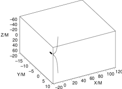
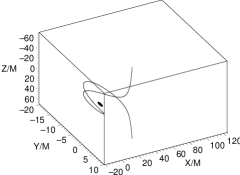
(a) T/M=0	(b) T/M=21.88
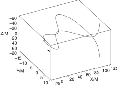
(c) T/M=41.31	(d) T/M=60.51

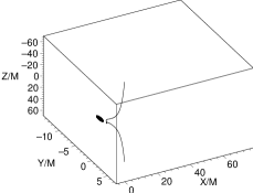
Figure 5: Real time profiles of the cosmic string: $v/c=0.995$, $a/M=1$ and $b/M=2.9$.

(a) T/M=0	(b) T/M=27.25
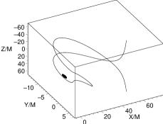
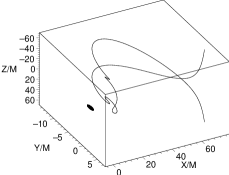
(c) T/M=44.76	(d) T/M=63.30

Figure 6: Real time profiles of the cosmic string: $v/c=0.995$, $a/M=1$ and $b/M=2.55$.

(a) T/M=15.13	(b) T/M=30.19
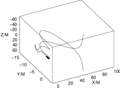
(c) T/M=40.10	(d) T/M=48.57
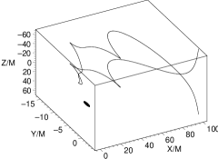
(e) T/M=58.87	(f) T/M=95.65

Figure 7: Real time profiles of the cosmic string: $v/c=0.995$, $a/M=1$ and $b/M=2.4125$.

As we saw in the previous section the critical impact parameter curve is more complicated in the ultrarelativistic regime for a rapidly rotating black hole. This can be better understood from the way the string is scattered in the critical regime. Figures 6–7 illustrate this. Each of the figures contains a set of snapshots made at some moment of coordinate time $T$. We call such a snapshot a real time profile. The time is given in units of $GM/c^{3}$. $T=0$ corresponds to the moment when the parts of the string located far from the black hole (where the spacetime is practically flat) pass the $X=0$ plane. The black hole event horizon is depicted as a black spot. It should be noted that the scales along different axes are different. That is the reason why instead of a round circle the spot representing the black hole event horizon looks like an ellipse.

There are two basic modes how a string can escape. In the ”standard” mode the string passes the black hole with its the center partially wrapped around it (figure 6, (a)–(b)). As the rest of the string escapes the central part unwraps and the string escapes to infinity (figure 6, (c)–(d)). As we lower the impact parameter the central part wraps more around the black hole and ultimately it does not have enough time to unwrap and it gets captured. However, if we lower the impact parameter under a certain value the string can escape again. Now the mechanism is different. In this ”alternative” mode the string wraps around the black hole as in the ”standard” mode (figure 6, (a)–(b)) but this time instead of unwrapping the black hole slips through the open coil (figure 6, (c)–(d)). For even smaller values of the impact parameter this mechanism breaks down eventually and the string is captured again. Although it is possible that there exists another ”island of escape” below the lowest branch of the critical impact parameter curve we did not observe it in our simulations.

To have a better picture of the two different escape modes we created 3 MAPLE animations, each corresponding to one of the figures 6–7. These can be found at the URL http://www.phys.ualberta.ca/~frolov/CSBH. Note that the animations show only the central part of the string. In the animations the rate of time is “slowed down” when the string is close to the black hole in order to make the details of the string behavior more clear. For this reason it seams that the string starts moving more rapidly when all its parts leave the proximity of the black hole.

Interesting features of the string structure are connected with wrapping effect, that is, when the central part of the string rotates around the black hole at the angle greater than $2\pi$. Such wrapping type of motion is characteristic for the motion of the ultrarelativistic particles in the regime close to capture. The tension of the string makes this effect less profound. One can expect that for highly ultrarelativistic motion it occurs even for a non-rotating black hole. We do not see this effect in our simulations since we can not perform sufficiently accurate calculations for ultrarelativistic velocities beyond $\beta\approx 4.0$. The dragging on effect connected with the rotation of the black hole makes this effect more profound. Figure 7 shows real time profiles for the string which ”wraps” around the black hole. It is interesting that during this process sharp spikes are formed in the string profiles.

4.2 Late time scattering data

For near critical scattering the central part of the string spends some time in the vicinity of the black hole while the further located parts of the string keep moving forward. After the central part of the string leaves the black hole vicinity the string as a whole is moving away from the black hole with the central part excitations propagating along the string. The combination of these effects results in quite a rich structure of the late time string profiles. Figures 9-11 illustrate this.

(a)	(b)
(c)	(d)

Figure 8: Late time profiles of the cosmic string: $v/c=0.995$, $a/M=1$ and $b/M=2.9$, $T/M=7446.47$.

(a)	(b)
(c)	(d)

Figure 9: Late time profiles of the cosmic string: $v/c=0.995$, $a/M=1$ and $b/M=2.55$, $T/M=7448.56$.

(a)	(b)
(c)	(d)

Figure 10: Late time profiles of the cosmic string: $v/c=0.995$, $a/M=1$ and $b/M=2.4125$, $T/M=4991.53$.

(a)	(b)
(c)	(d)

Figure 11: Late time profiles of the cosmic string: $v/c=0.995$, $a/M=0$ and $b/M=5.17$, $T/M=5209.56$.

Each of these figures consists of four plots. They demonstrate the form of the string some time after it passes close to the black hole. The black hole left behind the string is not shown. We show only that part of the string near the center which contains interesting details. The strings depicted on the figures 9–11 differ only by their initial impact parameter $b$. They are scattered by an extremal black hole in the prograde direction. For comparison figure 11 shows the late time profiles of a critically scattered string by a Schwarzschild black hole. Plots (a) show the real time 3-dimensional space profile of the string, while plots (b), (c), and (d) show 2-dimensional projections onto the planes $X$-$Y$, $Y$-$Z$, and $X$-$Z$, respectively. One can easily observe that at this relatively late time when the interaction with the black hole becomes weak the part of the string close to the center looks practically as a segment of a straight line. This property is also characteristic for a generic (non-critical) string scattering. Namely, it was demonstrated that for this case as a result of scattering the central part of the string ‘shifts’ into the $Y$-direction and a new ‘phase’ is formed. This new phase is that region of the string which is moving in the plane parallel to the initial one, but is displaced by some value $\Delta Y$ in the $Y$-direction. The length of the string segment in the new phase grows with the velocity of light, the transition layers being kink-like profiles. It is remarkable that a similar picture is valid also in the critical regime, as one can see by comparing plots (c) at figures 9–11. An important new feature is the possibility that the points with maximum shift in $Y$ direction may be located not at the center of the string, but slightly aside. Figure 9 (c) shows that there are two such points located symmetrically with respect to the center.

The $X$-$Z$–profiles (plots (d) at figures 9-11) are also quite regular and resemble similar profiles for a non-critical scattering. On the contrary, the $X$-$Y$–profiles (plots (b) at figures 9-11) are rich of details. The spikes in the string shape are most profound in this projection. All these details are connected with a simple fact that the central part of the string spends considerable time moving near the black hole, while the other parts of the string are moving away practically with the velocity of light. The profiles are sharper for the strings scattered by a rotating black holes. One can expect that by fine tuning the impact parameter one might be able to obtain string configurations which remain ‘glued’ to the vicinity of the black hole for arbitrary long time. But one can also expect that such solutions are very unstable, so that a tiny change of the impact parameter either results in the capture of the string or in its earlier escape. This situation is similar to the one discussed in [16]. The paper demonstrated that axially symmetric motion of a circular string in the gravitational field of Schwarzschild black hole is chaotic. One can make a conjecture that the near-critical scattering of the cosmic string is also chaotic.

5 Coil formation

(a)	(b)
(c)	(d)
(e)	(f)

Figure 12: Coil formation regions for prograde and retrograde scattering of the string.

There exists a special regime of the string scattering when after passing nearby a black hole the string forms a coil. A coil arises when the function $Z(\tau,\sigma)$ looses its property to be a monotonous function of $\sigma$ at fixed $\tau_{0}$. In this case there exist two different values $\sigma_{0}$ and $-\sigma_{0}$ for which the value of $Z$ is zero, $Z(\tau_{0},\sigma_{0})=Z(\tau_{0},-\sigma_{0})=0$. Since all other coordinates are symmetric functions of $\sigma$, the point $(\tau_{0},\pm\sigma_{0})$ is in fact a point of the string self intersection. A coil exists for some finite time interval from $\tau_{i}$ till $\tau_{f}$. At the end points of this interval $\partial_{\sigma}Z|_{\sigma=0}=0$.

It should be emphasized that, because of the interconnection effect, for most of the string models any self-crossing of the string results in the formation of a loop. After this, the loop moves independently from the remaining part of the string. In our simulations we did not include this effect. For this reason, such details as a coil size and structure may not represent the real properties of the string after its self-intersection. On the other hand, before the intersection occurs the numerical simulation describes the correct picture. That is why we focus our attention on the form of the coil formation curve. This is a curve (or surface) in the space of parameters which separates the region without coils from the region with coils. The structure of the coil formation curve does not depend on the details of the loop formation process.

Figure 12 shows the regions of coil formation for different values of the rotation parameter $a$. This region lies below the coil formation curves shown in the pictures. From below this region is restricted by the critical impact parameter curve. For a point lying exactly on the coil formation curve one has $\tau_{i}=\tau_{f}=\tau_{*}$. It means that $\partial_{\sigma}Z|_{\sigma=0}$ has a local minimum at this point as a function of $\tau$ and hence

$$\partial_{\sigma}Z|_{(\sigma=0,\tau=\tau_{*})}=\partial_{\tau}\partial_{\sigma}Z|_{(\sigma=0,\tau=\tau_{*})}=0\,.$$ (5.1)

The plots presented in figure 12 demonstrate that the formation of coils occurs when a string moves with relativistic velocity. For the prograde motion the coil formation starts at $v/c\approx 0.6$ (see figure 12, (c) and (d)). For the retrograde motion the corresponding velocity is higher and reaches $v/c\approx 0.8$ for the extremally rotating black hole (see figure 12 (e) and (f)).

It is instructive to compare these results with the condition of the coil formation in the weak field approximation. In order to do this we need to solve the weak field equations (see [8]). We first solve these equations for the case when a straight string at some initial moment of time $\tau=0$ is located at $X=X_{0}$, where $X_{0}$ is a large distance of the string from the black hole. We obtain a unique solution of perturbed equations by assuming that the deflection of the string from the straight line vanishes at $\tau=0$. The problem can be solved analytically but the result is given by rather long expressions, so we do not reproduce it here. Instead, we consider a limit when $X_{0}\to-\infty$. To calculate the limit it is convenient to choose $X_{0}=(\tilde{\tau}-\tau)\sinh\beta$ and, while keeping $\tilde{\tau}$ finite, to send $\tau\to\infty$. The physical interpretation of the new time-like parameter $\tilde{\tau}$ is quite simple—at $\tilde{\tau}=0$ the string crosses the $X=0$ plane.

Omitting the terms vanishing in this limit we obtain

$$Z=\sigma+M\cosh\beta\ln\left(\frac{A_{-}B_{-}}{A_{+}B_{+}}\right)\,,$$ (5.2)

$$Y=b-M\sinh\beta\left[\arctan\left(\frac{b^{2}+\tilde{\tau}(\tilde{\tau}+\sigma)\sinh^{2}\beta}{b\sinh\beta\sqrt{{\tilde{\tau}}^{2}\sinh^{2}\beta+b^{2}+\sigma^{2}}}\right)+\right.$$

$$+\arctan\left(\frac{b^{2}+\tilde{\tau}(\tilde{\tau}-\sigma)\sinh^{2}\beta}{b\sinh\beta\sqrt{{\tilde{\tau}}^{2}\sinh^{2}\beta+b^{2}+\sigma^{2}}}\right)+$$

$$+\left.\arctan\left(\frac{(\tilde{\tau}+\sigma)\sinh\beta}{b\cosh\beta}\right)+\arctan\left(\frac{(\tilde{\tau}-\sigma)\sinh\beta}{b\cosh\beta}\right)\right]\,,$$ (5.3)

$$X=\tilde{\tau}\sinh\beta\,,$$ (5.4)

$$T=\tilde{\tau}\cosh\beta+M\ln\left(4\frac{B_{-}B_{+}}{A_{-}A_{+}}\right)+2M\ln(\tau\cosh^{2}\beta)\,,$$ (5.5)

with

$$A_{\pm}=b^{2}\cosh^{2}\beta+(\tilde{\tau}\pm\sigma)^{2}\sinh^{2}\beta\,,$$ (5.6)

$$B_{\pm}=\cosh\beta\sqrt{{\tilde{\tau}}^{2}\sinh^{2}\beta+b^{2}+\sigma^{2}}+\tilde{\tau}\sinh^{2}\beta\pm\sigma\,.$$ (5.7)

The divergent term $2M\ln(\tau\cosh^{2}\beta)$ in the expression for $T$ arises because the gravitational field at infinity falls down not rapidly enough.

It is easy to check that $Z$ is an antisymmetric function of $\sigma$, so that for example $Z_{,\sigma\sigma}|_{\sigma=0}=0$. To obtain the condition of the coil formation one needs first to calculate the derivatives $Z_{,\sigma}$ and $Z_{,\sigma\tilde{\tau}}$, and then solve the equations

$$Z_{,\sigma}|_{\sigma=0}=0\,,$$ (5.8)

$$Z_{,\sigma\tilde{\tau}}|_{\sigma=0}=0\,,$$ (5.9)

in order to determine $\tau_{*}$ and $b$ as functions of rapidity $\beta$. By calculating the derivatives we obtain

$$Z_{,\sigma}|_{\sigma=0}=1-2M\cosh\beta\left(\frac{1}{\rho\cosh\beta+\tilde{\tau}\sinh^{2}\beta}+\frac{2\tilde{\tau}\sinh^{2}\beta}{{\tilde{\tau}}^{2}\sinh^{2}\beta+b^{2}\cosh^{2}\beta}\right)\,,$$ (5.10)

$$Z_{,\sigma\tilde{\tau}}|_{\sigma=0}=2M\cosh\beta\sinh^{2}\beta\left(\frac{\tilde{\tau}\cosh\beta+\rho}{(\rho\cosh\beta+\tilde{\tau}\sinh^{2}\beta)^{2}\rho}-\frac{2(b^{2}\cosh^{2}\beta-{\tilde{\tau}}^{2}\sinh^{2}\beta)}{({\tilde{\tau}}^{2}\sinh^{2}\beta+b^{2}\cosh^{2}\beta)^{2}}\right)\,,$$ (5.11)

where

$$\rho=\sqrt{{\tilde{\tau}}^{2}\sinh^{2}\beta+b^{2}}\,.$$ (5.12)

We use MAPLE to make all the above computations and to solve equations (5.8)–(5.9). The solution is

$$b=2M\cosh\beta\,,\hskip 28.45274pt\tau_{*}=2M\cosh\beta\,.$$ (5.13)

The relation $b=2M\cosh\beta$ determines a coil formation curve. This result coincides with the one obtained earlier in [13] as a condition for coil formation for the ultrarelativistic ($\beta\to\infty$) motion of the string.

For comparison, we show the coil formation curves for a non-rotating black hole in figure 12 (a) as calculated by using the weak field approximation. The corresponding curve lies below the exact one. One can conclude that the strong field effects help the coil formation process.

6 Discussions

In this paper we described the results of study of capture of a long cosmic string by a rotating black hole and its critical scattering. Since both problems are very non-linear, we use numerical simulations. For capture and critical scattering of the string the effects connected with the rotation of the black hole are very profound. Partially it is connected with the fact that the dragging into rotation effect increases the velocity of the central part of the string (as seen by an external observer) for prograde scattering and decreases it for the retrograde scattering. Because it is easier to catch a slower moving object the critical impact parameter $b_{c}(v,a)$ is greater for retrograde motion than for the prograde one. We calculated the critical impact parameter as a function of velocity of the string and angular momentum of the black hole. These plots have interesting features for $v$ and $a/M$ close to 1. In this regime the central part of the string can spend a considerable amount of time moving in the black hole vicinity before it gets captured or escapes. This makes such a regime of critical scattering highly complicated. Since the system is non-linear, and there are two qualitatively different final states (capture and scattering) one can expect elements of chaotic behavior in this case. Such a chaotic behavior occurs for example in the axisymmetric case when a circular loop of a cosmic string moves in the Schwarzschild black hole metric [16].

One can also make the following observation. The internal geometry on the world-sheet of the string is described by a time dependent 2-dimensional metric. When the string crosses the event horizon of the bulk black hole, a region on the string surface is formed from where it is impossible to communicate with the parts of the string which are outside the bulk black hole event horizon. In other words, a two-dimensional black hole is created. The degrees of freedom living on the string surface, e.g. transverse string perturbations, propagate in this 2-dimensional spacetime with a 2-D black hole in it [17, 18]. From this ‘2-D point of view’ the scattering of the string with the critical impact parameter is an event at the threshold of the 2-D black hole formation. One can make a conjecture that a formation of a 2-D stringy hole obeys the scaling laws similar to the universal scaling laws numerically discovered by Choptuik [19] in the general theory of relativity. A similar effects for a world domain interacting with a black hole was discussed in [20, 21].

Acknowledgments:  This work was partly supported by the Natural Sciences and Engineering Research Council of Canada. One of the authors (V.F.) is grateful to the Killam Trust for its financial support. M.S. thanks FS Chia PhD Scholarship. The authors are grateful to Don Page for various stimulating discussions.

References

- [1] Vilenkin, A. and Shellard, E.P.S. Cosmic strings and other topological defects. (Cambridge Univ. Press, Cambridge) (1994).
- [2] Pogosian, L. and Vachaspati, T. Phys. Rev. D60, 083504 (1999).
- [3] Contaldi, C.R. E-print astro-ph/0005115 (2000).
- [4] Simatos, N. and Perivolaropoulos, L. Phys. Rev. D63, 025018 (2001).
- [5] Landriau, M. and Shellard, E. P. S. E-print astro-ph/0208540 (2002).
- [6] Bouchet, F.R., Peter, P., Riazuelo, A. and Sakellariadou, M. Phys. Rev. D65, 021301 (2002).
- [7] Garfinkle, D. and Will, C. Phys. Rev. D35, 1124 (1987).
- [8] De Villiers, J.P. and Frolov, V.P. Phys. Rev. D58, 105018(8) (1998).
- [9] Page, D.N. Phys. Rev. D58, 105026(13) (1998).
- [10] Page, D.N. Phys.Rev. D60, 023510 (1999).
- [11] Snajdr, M., Frolov, V.P. and De Villiers, J.P. Class. Quant. Gravity 19, 5987 (2002)
- [12] De Villiers, J.P. and Frolov, V.P. Int. J. Mod. Phys. D7 No. 6 (1998) 957-967.
- [13] De Villiers, J.P. and Frolov, V.P. Class. Quant. Gravity 16, 2403 (1999).
- [14] Misner, C.W., Thorne, K.S. and Wheeler, J.A. Gravitation (W.H. Freeman, San Francisco, 1973).
- [15] Frolov, V.P. and Novikov, I.D. Black Hole Physics: Basic Concepts and New Developments, Kluwer Acad. Publ., 1998.
- [16] Frolov, A.V. and Larsen, A.L. Class.Quant.Grav. 16 3717 (1999).
- [17] Frolov, V.P. and Larsen, A.L. Nucl.Phys. B449 149 (1995).
- [18] Frolov, V.P., Hendy, S. and Larsen, A.L. Phys.Rev. D54 5093 (1996).
- [19] Choptuik, M.W. Phys. Rev. Lett. 70, 9 (1993).
- [20] Christensen, M., Frolov, V.P. and Larsen A.L. Phys.Rev. D58 085008 (1998).
- [21] Frolov, V.P., Larsen, A.L. and Christensen, M. Phys.Rev. D59 125008 (1999).