Inflation and Oscillations of Universe in 4D Dilatonic Gravity

Abstract

We investigate the inflation of Universe in a model of four dimensional dilatonic gravity with a massive dilaton field $\Phi$. The dilaton plays simultaneously the roles of an inflation field and a quintessence field. It yields a sequential hyper-inflation with a graceful exit to asymptotic de Sitter space-time, which is an attractor, and is approached as $\exp(-\sqrt{3\Lambda^{obs}}\,ct/2)$. The time duration of the inflation is reciprocal to the the mass of the dilaton: $\Delta t_{infl}\sim m_{{}_{\Phi}}^{-1}$. The typical number of e-folds in the simplest model of this type is shown to be realistic without fine tuning.

PACS number(s): 04.50.+h, 04.40.Nr, 04.62.+v

I Introduction

We consider a specific 4D-dilatonic model of gravity (4D-DG) with a gravi-dilaton action F00 ; F02 :

$${\cal A}_{g,\Phi}=-{\frac{c}{2\kappa}}\int d^{4}x\sqrt{|{\bf g}|}\bigl{(}\Phi R+2\Lambda^{obs}\,U(\Phi)\bigr{)},$$ (1)

where $\kappa=8\pi G_{N}/c^{2}$ is the Einstein constant and $\Lambda^{obs}$ is the observed value of the cosmological constant. In our model we have only one unknown function – the cosmological potential $U(\Phi)$ – which has to be chosen to comply with all gravitational experiments and observations in laboratory experiments, in star systems, in astrophysics and cosmology. In addition it has to solve the inverse cosmological problem, namely, to determine $U(\Phi)$ that reproduces the time evolution of the scale parameter $a(t)$ in accordance with the Robertson-Walker (RW) model of Universe F00 ; F02 ). Further on we use cosmological units, in which the cosmological constant $\Lambda^{obs}$ equals one F00 ; F02 .

The dilaton field $\Phi$ is a quantity, reciprocal to the dimensionless gravitational factor $g$:   $\Phi=1/g$. As usual in our scalar-tensor theory of gravity of Brans-Dicke type, instead of the Newton gravitational constant $G_{N}$, we define the variable gravitational factor $G_{eff}(x)=G_{N}\,g(x)$ as a function of space-time coordinates $x=\{ct,{\bf x}\}$.

There exist different reasons for considering this model. For example, it appears in the five-dimensional Kaluza-Klein model, or, it can be produced in the low energy limit of string theory, by ignoring (yet unobserved) possible higher dimensions. (See for details and for references F02 .) The most physically relevant motivation for the use of a model with action (1) at present can be find in the attempts to develop a quantum version of Einstein gravity in four dimensional space-time QNLG .

Recently, a very promising discovery of the existence of a consistent quantum gravity in four dimensional space-time was made by Reuter Reuter . It confirms an early prediction by Weinberg that Einstein gravity in four dimensions may be ”asymptotically safe”, because of the existence of a fixed point of the renormalization-group equations, similar to the one in $2+\varepsilon$ dimensions Weinberg79 . Indeed, by making use of suitable Einstein-Hibert truncation, i.e., using action (1) with $\Phi=1$ and $U(\Phi)=1$ it has been proven that the four-dimensional possesses an ultra-violet fixed point and is asymptotically free. Then, as a result of the renormalization, one obtains a running gravitational constant $G$ and a cosmological constant $\Lambda$. In the case of quantum electrodynamics we have running electric charges, due to the cloud of virtual photons. In quantum gravity, a test body would be surrounded by a cloud of virtual gravitons. In contrast to electrodynamics though, the gravity is universal attractive and the effective mass of the body, as seen by a distant observer, is larger than it would be in absence of quantum effects. Hence, in quantum gravity we have an anti-screening effect, which entails the Newton constant and the cosmological constant becoming scale dependent quantities. As a result of the general relativistic invariance they become functions of space-time points.

We prefer to describe the above phenomena using the dilaton field $\Phi$ in action (1). This field encapsulates the space-time dependence of the corresponding parameters. The use of a cosmological potential $U(\Phi)$ of general form is known to be equivalent to the nonlinear gravity (NLG), described by a nonlinear (with respect to the space-time scalar curvature $R$) Hilbert-Einstein Lagrangian $L(R)$ in the action. (See F02 ; NLG for more details and for references.) At present, the form of this Lagrangian is complete unknown. The renorm-group analysis of the nonlinear terms in Reuter approach is still an open problem. It is clear that, in general, all coefficients in the different terms of the Taylor (or Laurent) series expansion of the function $L(R)$ will become running constants, as a result of quantum effects.

As shown in F00 ; F02 , the use of the cosmological potential $U(\Phi)$, as an alternative description of these nonlinear terms, is extremely useful. Indeed, one is able to formulate simple and clear physical requirements for this potential. For example, to have an unique physical de Sitter (classical) vacuum (dSV) in the theory, the function $U(\Phi)$ must have an unique positive minimum for positive values of the dilaton field $\Phi$. To avoid the non-physical negative values of the dilation field $\Phi$, the potential must increase to infinity for $\Phi\to+0$, etc. (See F02 .)

Here we use the simplest one-parameter potential:

$$U(\Phi)=\Phi^{2}+W(\Phi)=\Phi^{2}+{3\over{16}}p^{-2}_{{}_{\Phi}}\left(\Phi-{1\over\Phi}\right)^{2}\,$$ (2)

with such properties. The parameter $p_{{}_{\Phi}}$ is the dimensionless Compton length of the dilaton in cosmological units, defined by the equation $p^{2}_{{}_{\Phi}}=\Lambda^{obs}\,l_{{}_{\Phi}}^{2}$, where $l_{{}_{\Phi}}={\hbar\over{cm_{{}_{\Phi}}}}$ is the usual Compton length of the dilaton, and $m_{{}_{\Phi}}$ is the mass of the dilaton. To comply with all known facts in gravitational physics, astrophysics and cosmology the dilaton mass must obey the constraint equation $m_{{}_{\Phi}}>10^{-3}\rm eV$. This yields an extremely small value of the dimensionless parameter $p_{{}_{\Phi}}<10^{-30}$ F00 ; F02 .

The cosmological potential (2) corresponds to a non-polynomial Lagrangian for the equivalent NLG: $L(R;p_{{}_{\Phi}})\sim-f(R;p_{{}_{\Phi}})$. It is described in parametric form by the equations: $R={3\over{4}}p^{-2}_{{}_{\Phi}}\left({1/\Phi^{3}}-\Phi\right)-4\Phi$ and $f={3\over{8}}p^{-2}_{{}_{\Phi}}\left({3/\Phi^{2}}-\Phi^{2}-2\right)-2\Phi^{2}$, $\Phi\in(0,\infty)$. One can see that the physical branch of the function $f(R;p_{{}_{\Phi}})$ has a Taylor series expansion

$$f(R;p_{{}_{\Phi}})=R+2+1/3\,(R+4)(R+8)\,p_{{}_{\Phi}}^{2}+{\cal O}(p_{{}_{\Phi}}^{4})$$

and goes to the linear Einstein-Hilbert one $f(R;p_{{}_{\Phi}})\to R+2$ (in cosmological units) in the limit $p_{{}_{\Phi}}\to 0$, i.e., when $m_{{}_{\Phi}}\to\infty$. Hence, in this sense, our 4D-DG has the GR as a limiting case.

As seen in Fig. 1, for values of the scalar curvature $|R|\ll 1$ our model behaves like GR with standard Newton constant $G_{N}$. For $R\ll-1$ it behaves like GR with smaller effective gravitational constant, and for $R\gg 1$ – like GR with bigger effective gravitational constant:

$$G_{eff}|_{{}_{R\ll\!-1}}<G_{eff}|_{{}_{|R|\ll\!1}}\approx G_{N}<G_{eff}|_{{}_{R\gg\!1}}.$$

Figure 1:   The form of the function $f(R;p_{{}_{\Phi}})$ in the equivalent nonlinear gravity for different values of the parameter $p_{{}_{\Phi}}=1/10,1/20,1/30,...,0$.          

In the general case, one must consider a 4D-DG model with a matter sector and a gravi-dilaton sector. The investigation of the effect of the presence of matter in Reuter approach to quantum gravity was started in Percacci . Some general properties of 4D-DG model with matter were derived in F02 . In the present article we shell ignore the influence of matter for simplicity. Its presence yields a new important phenomena, which we intend to describe in a separate article.

II The Basic Equations for Robertson-Walker (RW) Universe in the 4D-Dilatonic Gravity

Consider RW adiabatic homogeneous isotropic Universe with

$$ds^{2}_{RW}=dt^{2}-a^{2}(t)dl^{2}_{k},$$

where $dl^{2}_{k}={\frac{dl^{2}}{1-kl^{2}}+l^{2}(d\theta^{2}+\sin^{2}\theta)d\varphi^{2}}$ (for $k=-1,0,1$). In our cosmological units the time $t$, and the scale parameter of Universe $a(t)$ are dimensionless.

For a free of matter Universe we obtain the following basic dynamical equations, governing the time evolution of the 4D-DG-RW model:

$${\frac{\ddot{a}}{a}}+{\frac{\dot{a}^{2}}{a^{2}}}+{\frac{k}{a^{2}}}={\frac{1}{3}}\,U_{{,_{\Phi}}}(\Phi),$$

$${\frac{\dot{a}}{a}}\dot{\Phi}+\Phi\left({\frac{\dot{a}^{2}}{a^{2}}}+{\frac{k}{a^{2}}}\right)={\frac{1}{3}}U(\Phi).$$ (3)

The dynamical equation for the dilaton $\Phi$ is

$$\ddot{\Phi}+3{\frac{\dot{a}}{a}}\dot{\Phi}+V_{,_{\Phi}}(\Phi)=0$$ (4)

and

$$V(\Phi)={1\over 2}\,p^{-2}_{{}_{\Phi}}\left(\Phi+{1\over\Phi}-2\right)$$ (5)

is the dilatonic potential F02 .

II.1 First Normal Form of the Dynamical Equations

Introducing a new regularizing variable $\tau$ by $dt=Hd\tau$ and the notations $x_{1}:=H^{2}\geq 0$, $x_{2}:=\Phi>0$, $x_{3}:=\ln a$ (where $H=\dot{a}/a$ is the Hubble parameter) we can rewrite the basic system (3) in standard normal form:

$${\frac{d}{d\tau}}{\bf x}={\bf f(x)}\,,$$ (6)

where ${\bf x},{\bf f}\in{\cal R}^{(3)}$ are three-dimensional vector-columns with components $\{x_{1},x_{2},x_{3}\}$ and $\{f_{1},f_{2},f_{3}\}$, respectively, and

$$f_{1}=4x_{1}\left(Z_{1}(x_{2})-x_{1}-ke^{-2x_{3}}/2\right),\hskip 31.2982pt$$

$$f_{2}=x_{2}\left(Z_{2}(x_{2})-x_{1}-ke^{-2x_{3}}\right),\hskip 46.94687pt$$

$$f_{3}=x_{1}.\hskip 152.22241pt$$ (7)

Here the quantities

$$Z_{1}(\Phi)={\frac{1}{6}}U{\!,_{\Phi}}(\Phi)=Z_{2}(\Phi)+{\frac{1}{4}}V_{\!,_{\Phi}}/\Phi,$$

$$Z_{2}(\Phi)={\frac{1}{3}}U(\Phi)/\Phi={\frac{1}{3}}\Phi+{\frac{1}{3}}W/\Phi.\hskip 11.38092pt$$ (8)

are regarded as functions of $x_{2}=\Phi$.

Now one can derive another important relation of a pseudo-energetic type by using Eq. (4). The qualitative dynamics of its solutions is determined by the function

$$\eta={1\over 2}\dot{\Phi}^{2}+V(\Phi).$$ (9)

This function plays the role of a (non conserved) energy-like function for the dilaton field $\Phi$ in the 4D-DG-RW Universe and obeys the equation

$${d\over{d\tau}}\eta=-3\left({d\over{d\tau}}\Phi\right)^{2}\leq 0.$$ (10)

As seen from this equation, the quantity $\eta$ defines a Lyapunov function in a generalized sense in our model of Universe, filled only with vacuum energy. In this case the parameter $\eta(\tau)$ is a monotonically decreasing function of the time $\tau$. One can show, that the same relations are valid for the case of ultra relativistic matter, when the trace of energy-momentum tensor equals zero and the function $\eta$ is a Lyapunov function for the corresponding generalization of the normal system of ordinary differential equations (6) F02 .

All solutions to the system (6) must cross the surfaces of level $\eta=const$ of this function and go into its interior. The form of this two-sheeted surfaces is described explicitly by the equation:

$$H={1\over\Phi}\sqrt{\eta\!-\!V\!+\!\Phi\Delta\pm\sqrt{\left(\eta\!-\!V\right)\left(\eta\!-\!V\!+\!2\Phi\Delta\right)}}.$$ (11)

Here $\Delta={1\over 3}U-k{\Phi\over{a^{2}}}$. A typical geometrical form of a level-surface of the function $\eta$ in absence of matter for the simple potential $V=V(\Phi)$ (5) is shown in Fig. 2 – for $k=1$, and in Fig. 3 – for $k=-1$. For $k=0$ the function (11) does not depend on the scale factor $a$ and the corresponding surface is a simple cylinder.

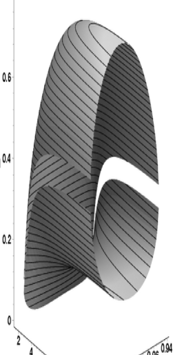
Figure 2:   Level surface of the Lyapunov function $\eta$ – Eq. (9) for the potential $V(\Phi)$ – Eq. (2) and $k=+1$.          

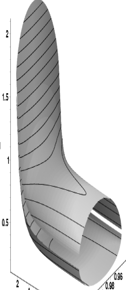
Figure 3:   Level surface of the Lyapunov function $\eta$ – Eq. (9) for the potential $V(\Phi)$ – Eq. (2) and $k=-1$.          

One can see two main specific features of the behavior of this surface:

1) At small values of the RW scale factor $a\sim 0$ the form of the Lyapunov surface depends strongly on the sign of 3-space scalar curvature: For $k=+1$ we have a semi-infinite curved cylinder with a closed bottom, which goes down to values $H=0$ in ”vertical” direction. In contrast, for $k=-1$ we have on both sides an infinite curved cylinder which goes up to values $H=\infty$ in ”vertical” direction. At the end, for $k=0$ we have a simple straight ”horizontal” cylinder.

2) For all values $k=0,\pm 1$ and $a\to\infty$ we have infinitely long “horizontal” tube along the $a$-axes. The solutions that enter the inner part of the $\{a,\Phi,H\}$-space through the Lyapunov surface, in this area go to de Sitter asymptotic regime winding around the axis of the tube and approaching it for $t\to\infty$.

The analytical behavior of the solutions in the completely different regimes at $a\sim 0$, and at $a\gg 1$, as well as the transition of given solution to asymptotically de Sitter regime will be described below in more detail.

II.2 Second Normal Form of the Dynamical Equations

We need one more normal form of the dynamical equations to study the behavior of their solutions for $x_{1},x_{2}\to\infty$. The standard techniques for investigation of the solutions in this limit show that the infinite point is a complex singular point, and one has to use the so called $\sigma$-process Arnold to split this singular point into elementary ones. This dictates the following change of variables:

$$x_{1}={\frac{3}{16}}p_{{}_{\Phi}}^{-2}z^{-4}g^{-4},\,\,\,x_{2}=g^{-1},\,\,\,t={\frac{4}{\sqrt{3}}}\,p_{{}_{\Phi}}\Theta\,,$$ (12)

which transforms the equations (6) with right hand sides (7) into a new system:

$$g^{\prime}=g\,{\cal D},\,\,\,z^{\prime}=z{\cal Z},\,\,\,\Theta^{\prime}=z^{2}g^{2}$$ (13)

where the prime denotes differentiation with respect to the variable $x_{3}$ and

$${\cal D}(g,z,a;p_{{}_{\Phi}}^{2},k) = 1-{\frac{1}{3}}z^{4}g^{5}w(g)$$

$$- \left(\!{\frac{4p_{{}_{\Phi}}}{3}}\!\right)^{\!2}\!\!g^{3}z^{4}\!\left(\!1\!-\!3g{\frac{k}{a^{2}}}\!\right)\!$$

$$= {\cal D}_{0}(g,z)\!+\!{\cal O}_{2}(p_{{}_{\Phi}}^{2})$$

$${\cal Z}(g,z,a;p_{{}_{\Phi}}^{2},k) = {\frac{1}{4}}z^{4}g^{7}v{,_{g}}(g)$$ (14)

$$- \!{\frac{3}{2}}\left(\!{\frac{4p_{{}_{\Phi}}}{3}}\!\right)^{\!2}\!g^{4}z^{4}\!\left({\frac{k}{a^{2}}}\!\right)\!$$

$$= \!{\cal Z}_{0}(g,z)\!+\!{\cal O}_{2}(p_{{}_{\Phi}}^{2})\,.$$

Here we have introduced the functions $v(g)\!=\!{\frac{16}{3}}p_{{}_{\Phi}}^{2}\!V({\frac{1}{g}})$ and $w(g)\!=\!{\frac{16}{3}}p_{{}_{\Phi}}^{2}\!W({\frac{1}{g}})$ which do not depend on the parameter $p_{{}_{\Phi}}$ and are simply related: $w=3/2g^{-2}\int_{1}^{g}g^{3}dv$. The functions ${\cal D}$ and ${\cal Z}$ are defined according to the formulae

$${\cal D}={\frac{d(\ln g)}{d(\ln a)}}\,,\quad{\cal Z}={\frac{d(\ln z)}{d(\ln a)}}\,.$$ (15)

The representation (14) shows that one can develop a simple perturbation theory for the highly nonlinear system (13) using the extremely small parameter $p_{{}_{\Phi}}^{2}$ as a perturbation parameter.

From the dynamical equations (6), (7) and (13), one easily obtains the following contour-integral representation for the number of e-folds ${\cal N}$ and for the elapsed time $\Delta t_{\cal N}={\frac{4}{\sqrt{3}}}\,p_{{}_{\Phi}}\Theta_{\cal N}$:

$${\cal N}(p_{{}_{\Phi}}^{2},k)\!=\!\int_{\tau_{in}}^{\tau_{fin}}\limits H^{2}(\tau)d\tau\!=\!\!\int_{{\cal C}_{in}^{fin}}\limits\!{\frac{dg/g}{{\cal D}(g,z,a;p_{{}_{\Phi}}^{2},k)}},$$ (16)

and

$$\Theta_{\cal{}_{N}}(p_{{}_{\Phi}}^{2},k)=\int_{{\cal C}_{in}^{fin}}\limits\!{\frac{z^{2}g\,dg}{{\cal D}(g,z,a;p_{{}_{\Phi}}^{2},k)}}.$$ (17)

Here, a start from some initial (in) state of the 4D-DG-RW Universe, followed by a motion along the contour ${\cal C}_{in}^{fin}$ (determined by corresponding solution of system (13)), and an end at some final (fin) state, are assumed.

III General Properties of the Solutions in the 4D-DG RW Universe

III.0.1 Properties of the Solutions in a Vicinity of dSV

Let us first consider the simplest case when $k=0$. The system (6) in this case splits into a single equation for $x_{3}$, which is solved by the monotonic function $x_{3}(\tau)=x_{3}^{0}+\int_{\tau_{0}}^{\tau}x_{1}(\tau)d\tau$, and the independent of $x_{3}$ system

$${\frac{d}{d\tau}}{x_{1}}=4x_{1}\left(Z_{1}(x_{2})-x_{1}\right),$$

$${\frac{d}{d\tau}}{x_{2}}=\,\,x_{2}\left(Z_{2}(x_{2})-x_{1}\right).\hskip 0.0pt$$ (18)

Now it is clear that the curves $\hat{x}_{1}=Z_{1}(\hat{x}_{2})$ and $\check{x}_{1}=Z_{2}(\check{x}_{2})$ are the zero-isoclinic lines for the solutions of (18). These curves describe the points of local extrema of the functions $x_{1}(\tau)$ and $x_{2}(\tau)$, respectively, in the domain $x_{1,2}>0$. Because of the condition $U(\Phi)>0$ and the existence of a unique minimum of the cosmological potential, these lines have a unique intersection point – a de Sitter vacuum (dSV) state F02 with $\bar{x}_{1}=1/3$, $\bar{x}_{2}=1$. This singular point represents the standard de Sitter solution, which in usual variables reads

$$\bar{H}=1/\sqrt{3},\,\,\,\bar{\Phi}=1,\,\,\,a(t)=a_{0}\exp(t/\sqrt{3}).$$ (19)

One can see the typical behavior of the solutions of the system (18) in the domain $x_{1,2}>0$, together with the curves $Z[1]:=\{\hat{x}_{1}=Z_{1}(\hat{x}_{2})\}$, and $Z[2]:=\{\check{x}_{1}=Z_{2}(\check{x}_{2})\}$, in Fig.4, where the corresponding phase portrait is shown for the case of the potentials (2) and $p_{{}_{\Phi}}=1/4$.

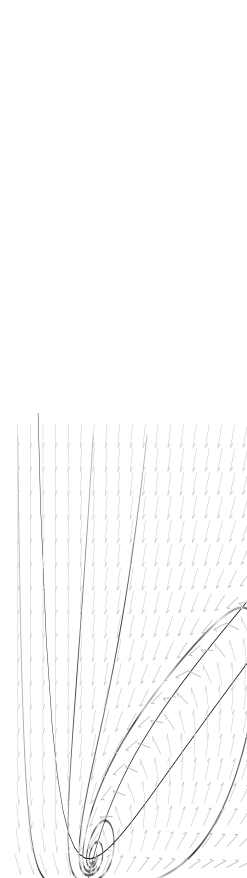
Figure 4:   A typical phase portrait of the system (18). The parts of solutions with the same color are covered by the Universe for equal $\tau$-intervals.          

Consider the solutions of the system (18) of the form $x_{1,2}(\tau)=\bar{x}_{1,2}+\delta x_{1,2}(\tau)$ that are close to dSV, i.e., with $|\delta x_{1,2}(\tau)|\ll 1$. Using the relations

$$V(1)=0,\,\,\,V{\!,_{\Phi}}(1)=0,\,\,\,V{\!,_{\Phi\Phi}}(1)=p^{-2}_{{}_{\Phi}};\hskip 28.45274pt$$

$$U(1)=1,\,\,\,U{\!,_{\Phi}}(1)=2,\,\,\,U{\!,_{\Phi\Phi}}(1)=2\left(1+{3\over 4}p^{-2}_{{}_{\Phi}}\right)\,,$$ (20)

which describe the general properties of de Sitter vacuum state (with $\bar{\Phi}=1$) in 4D-DG F02 , one obtains in linear approximation

$$\delta x_{1}(t)=\delta x_{1}^{0}\,\exp\!\left({-{\frac{\sqrt{3}}{2}}t}\right)\cos\left(\omega_{{}_{\Phi}}t\right),\hskip 39.83368pt$$

$$\delta x_{2}(t)\!=\!{\frac{3}{2}}{\frac{p_{{}_{\Phi}}\delta x_{1}^{0}}{\sqrt{p_{{}_{\Phi}}^{2}\!+\!{\frac{3}{4}}}}}\exp\!\left(\!{-{\frac{\sqrt{3}}{2}}t}\!\right)\!\cos\left(\omega_{{}_{\Phi}}t\!-\!\psi_{{}_{\Phi}}\right)$$

$$\delta x_{3}(t)\!=\!\delta x_{3}^{0}\!+\!\sqrt{3}p_{{}_{\Phi}}\delta x_{1}^{0}\exp\!\left(\!{-{\frac{\sqrt{3}}{2}}t}\!\right)\!\times\hskip 34.14322pt$$

$$\bigl{(}\cos\left(\omega_{{}_{\Phi}}t\!-\!\psi_{a}\right)-\cos\left(\psi_{a}\right)\bigr{)}\,,$$ (21)

where

$$\omega_{{}_{\Phi}}=\sqrt{p_{{}_{\Phi}}^{-2}-3/4}\,,\hskip 42.67912pt$$

$$\tan\psi_{{}_{\Phi}}={\frac{2\sqrt{3}}{5}}\,\omega_{{}_{\Phi}},\,\,\,\tan\psi_{a}=-{\frac{2\sqrt{3}}{3}}\,\omega_{{}_{\Phi}},$$ (22)

$\delta x_{1}^{0}=\delta x_{1}(0)$ is the small initial amplitude of $\delta x_{1}(t)$, and the solution for the deviation $\delta x_{3}(t)$ has been added for completeness and for later use.

The frequency $\omega_{{}_{\Phi}}$ is a real and positive number if $p_{{}_{\Phi}}<2/\sqrt{3}$. According to the estimate $p_{{}_{\Phi}}<10^{-30}$, in 4D-DG we have $\omega_{{}_{\Phi}}\geq 10^{30}$ in cosmological units, or $\omega_{{}_{\Phi}}\geq 10^{3}\,{\rm GHz}$ in usual units, and $\psi_{{}_{\Phi}}\approx\pi/2\approx-\psi_{a}$.

Thus, we see that the de Sitter vacuum is a stable focus in the phase portrait of the system (18). For $k=0$ all solutions of this system that lie in a small enough vicinity of dSV oscillate with an ultra-high frequency $\omega_{{}_{\Phi}}$ (22), and approach dSV in the limit $t\to\infty$.

One can generalize this statement for the case of arbitrary $k=0,\pm 1$ F02 . This turns out to be true even in the presence of nonzero matter energy-density terms. Then we see that one important general prediction for the 4D-DG-RW Universe is the existence of ultra-high dilatonic oscillations with frequency $\omega_{\Phi}$ (22) in 3-spaces with any curvature and in the presence of any kind of normal matter F02 .

If $p_{{}_{\Phi}}\geq 2/\sqrt{3}$, i.e., if $m_{{}_{\Phi}}\sim 10^{-33}\,{\rm eV}$ (as in inflation models with a slow-rolling scalar field and in quintessence models C ; inflation ; Q ), the above ultra-high dilatonic oscillations do not exist in the 4D-DG-RW Universe. In this case, the frequency $\omega_{{}_{\Phi}}$ becomes imaginary and, instead of a stable focus, we have an unstable saddle point in the phase portrait of the system (18). Such a situation was considered first in Starobinsky80 in a different model of nonlinear gravity based on a quadratic with respect to scalar curvature $R$ gravitational Lagrangian, but with some additional terms that originate from quantum fluctuations in curved space-time QNLG . These additional terms are related to the Weyl conformal curvature and therefore vanish in the case of RW metric, but yield an essentially different theory in other cases. Therefore, for RW Universe the model described in Starobinsky80 is equivalent to 4D-DG with a quadratic in the field $\Phi$ cosmological potential. Such a potential is non-physical, because it admits negative values of the dilaton field $\Phi$, i.e., of the gravitational constant.

An immediate consequence of the above consideration is the existence of ultra-high frequency oscillations of the effective gravitational factor $G_{eff}=G_{{}_{N}}/\Phi$, accompanied with an extremely slow exponential decrease of its amplitude $\sim\exp\left(-{\frac{1}{2}}\sqrt{3\Lambda^{obs}}\,ct\right)$ (in usual units). One obtains $\bar{H}^{2}/H^{2}_{0}=\Omega_{\Lambda}$ and $\delta H^{2}_{0}={\frac{1}{3}}{\frac{1-\Omega_{\Lambda}}{\Omega_{\Lambda}}}$. Hence, at the present epoch with $\Omega_{\Lambda}\approx{\frac{2}{3}}$, we have $\delta x_{1}^{0}\approx{\frac{1}{6}}$. Then the second equation of the system (21) gives

$$g(t)\approx 1-p_{{}_{\Phi}}{\frac{\sqrt{3}}{2}}\exp\!\left({-{\frac{\sqrt{3}}{2}}t}\right)\cos\left(\omega_{{}_{\Phi}}t-\psi_{{}_{\Phi}}\right)\,,$$ (23)

where we have introduced a dimensionless gravitational factor, $g(t)={{G_{eff}(t)}/{G_{{}_{N}}}}=1/\Phi(t)$.

Because of the extremely small amplitude $\!p_{{}_{\Phi}}\!\leq\!10^{-30}$, these variations are beyond the possibilities of present-day experimental techniques.

In contrast, the oscillations of the Hubble parameter $H$ have a relatively big amplitude $\delta H_{0}=\sqrt{\delta x_{0}}\approx 0.4$, and the same huge frequency $\omega_{{}_{\Phi}}$, as the oscillations of gravitational factor. It is very interesting to find possible observational consequences of such a phenomenon.

High frequency oscillations of the effective gravitational factor were considered first in the context of Brans-Dicke field with a BD parameter $\omega>1$ in Steinhardt . These oscillations were induced by an independent inflation field, but the analysis of the existing astrophysical and cosmological limits on the oscillations of $G_{eff}(t)$ is applicable to our 4D-DG model as well. The conclusion in Steinhardt is that the oscillations in the considered frequency-amplitude range, being proportional to $\dot{g}/(gH)$, do not affect the Earth-surface laboratory measurements, Solar System gravitational experiments, stellar evolution, and nucleosynthesis, but can produce significant cosmological effects because the frequency is very large and the Hubble parameter is small (in usual units). It can be seen explicitly from Eq. (21) that this is precisely what happens in 4D-DG, although in it the oscillations are self-induced.

As stressed in Steinhardt , despite the fact that the variations of the type (23) have extremely small amplitudes, they can produce significant cosmological effects because of the nonlinear character of gravity. In the case of free of matter Universe the 4D-DG version of the formula, analogous to the one in the first of references Steinhardt , is

$$H={\frac{1}{2}}{\frac{\dot{g}}{g}}\pm\sqrt{{\frac{1}{4}}\left({\frac{\dot{g}}{g}}\right)^{2}+{\frac{1}{3}}gU-{\frac{k}{a^{2}}}}\,.$$ (24)

Being a direct consequence of Eq. (3), this formula shows that, after averaging of the oscillations, the term ${{\dot{g}}/g}$ has a non-vanishing contribution because it enters the Hubble parameter (24) in a nonlinear manner. A more detailed mathematical treatment of this new phenomenon in 4D-DG is needed to derive reliable conclusions. The standard averaging techniques for differential equations with fast oscillating solutions and slowly developing modes seem to be the most natural mathematical method for this purpose, but the applications of these techniques to 4D-DG lie beyond the scope of the present article.

IV Inflation in 4D-DG-RW Universe

Having in mind that: 1) the essence of the inflation is a fast and huge re-scaling of the Universe C ; inflation , and 2) the dilaton is the scalar field determining the scales in Universe, it seems natural to relate these two fundamental physical notions instead of inventing some specific “inflation field”. In this section we show that our 4D-DG model indeed offers such a possibility.

IV.1 The Phase-Space Domain of Inflation

As seen from the phase portraits in Fig. 4–5, for values $H\geq H_{crit}$ and $\Phi\geq\Phi_{crit}$, the ultra-high-frequency-oscillations do not exist. The evolution of the Universe in this domain of the phase space of the system (3) reduces to some kind of monotonic expansion, according to the equation ${\frac{d}{d\tau}}x_{3}=H^{2}>0$. We call this expansion an inflation. As we shall see, it indeed has all needed properties to be considered as an inflation phenomenon.

The transition from inflation to high-frequency oscillations is a nonlinear phenomenon, and we will describe it in the present article very briefly. Here our goal is to have some approximate criteria for determining the end of the inflation. It is needed for evaluation of the basic quantities that describe the inflation.

As seen from Eq. (21), the amplitude, $\delta\Phi_{0}$, of the oscillations of $\Phi$ is extremely small compared with the amplitude $\delta H^{2}$ of the oscillations of $H^{2}$:   $\delta\Phi_{0}\lesssim{\frac{3}{2}}p_{{}_{\Phi}}/\sqrt{p_{{}_{\Phi}}^{2}+{\frac{3}{4}}}\,\delta H_{0}^{2}$. An obvious estimate for the amplitude $\delta H_{0}^{2}$ is $\delta H_{0}^{2}\leq 1/3\,(=\bar{H}^{2})$. Then, for $p_{{}_{\Phi}}\leq 2/\sqrt{3}$ (which is the condition for existence of oscillations), we obtain $\delta\Phi_{0}\lesssim\delta H_{0}^{2}\lesssim 1/3$. The last estimate is indeed very crude for the physical model at hand, in which $p_{{}_{\Phi}}\leq 10^{-30}$. This consideration produces the constraint $H_{crit}\lesssim\sqrt{2/3}$ and $\Phi_{crit}\lesssim 4/3$, but, taking into account the extremely small value of $p_{{}_{\Phi}}$, we will use for simplicity the very crude estimate $H_{crit},\Phi_{crit}\sim 1$.

Now it becomes clear that the study of the inflation requires considering big values of the variables $x_{1,2}$, i.e., using the second normal form (13) of the dynamical equations.

IV.2 The Behavior of the Solutions Near the Beginning

IV.2.1 The Case $k=0$

Let us consider first the case $k=0$. From Eq. (13) one obtains the simple first order equation

$${\frac{dz}{dg}}={\frac{z^{5}g^{6}}{4}}{\frac{v_{,_{g}}(g)}{{\cal D}(g,z;p_{{}_{\Phi}}^{2})}}$$ (25)

with

$${\cal D}(g,z;p_{{}_{\Phi}}^{2})=1-{\frac{1}{3}}z^{4}g^{5}u(g)=\hskip 85.35826pt$$

$$1\!-\!{\frac{1}{3}}z^{4}g^{5}w(g)\!-\!\left(\!{\frac{4p_{{}_{\Phi}}}{3}}\!\right)^{\!2}\!\!g^{3}z^{4}\!=\!{\cal D}_{0}(g,z)\!+\!{\cal O}_{2}(p_{{}_{\Phi}}^{2}),\,\,\,\,$$ (26)

where $u(g)={\frac{16}{3}}p_{{}_{\Phi}}^{2}U(1/g)$.

One can easily prove that the solutions of Eq. (18) have important general properties for small values of $g$. For the potentials (5) we obtain

$${\cal Z}_{0}(g,z)=-{\frac{2z^{4}}{3}}g^{5}\left(1-g^{2}\right)$$ (27)

and

$${\cal D}_{0}(g,z)\!=\!1\!-\!{\frac{z^{4}}{3}}g^{3}\left(1-g^{2}\right)^{2}.$$ (28)

Hence, $\lim_{g\to 0}{\cal D}_{0}(g,z)=1$. Then, taking into account the leading terms, we obtain from Eq. (13), (15), (17), (25), and (26) the following results in the limit $g\to 0$:

$$a(g)\sim g,\hskip 147.95424pt$$

$$z(g)\!=\!z_{0}\!-{\frac{2}{15}}\,z_{0}^{5}g^{5}+{\cal O}(g^{6}),\hskip 65.44142pt$$

$$t(g)\!=\!{\frac{2p_{{}_{\Phi}}}{\sqrt{3}}}z_{0}^{2}g^{2}\!+\!{\cal O}(g^{3}).\hskip 86.78099pt$$ (29)

When solved with respect to the time $t$, these formulae give

$$a(t)\sim\left({\frac{t}{p_{{}_{\Phi}}}}\right)^{1/2}\!\!,\,\,\,g(t)={\frac{1}{z_{0}}}\left({\frac{\sqrt{3}}{2p_{{}_{\Phi}}}}t\right)^{1/2}\!\!+{\cal O}(t),$$

$$z(t)=z_{0}-{\frac{2}{15}}\left(\!{\frac{\sqrt{3}}{2p_{{}_{\Phi}}}}t\!\right)^{5/2}+{\cal O}(t^{3}).\,\,\,$$ (30)

IV.2.2 The Case $k=\pm 1$

Now, the equations (13) do not split into a two-dimensional subsystem and an independent differential equation and must be considered as a true three-dimensional system. The expansion of its solutions in a Taylor series with respect to the variable $a$ is

$$g(a)=g_{1}\,a+{\cal O}(a^{2}),\hskip 59.75095pt$$

$$z(a)=z_{0}-{\frac{4}{3}}\,k\,p_{{}_{\Phi}}^{2}\,g_{1}^{4}\,a^{2}+{\cal O}(a^{3}),\,\,\,$$

$$t(a)={\frac{2}{\sqrt{3}}}\,p_{{}_{\Phi}}\,z_{0}^{2}\,g_{1}^{2}\,a^{2}+{\cal O}(a^{3}),\hskip 17.07182pt$$ (31)

with an arbitrary constants $g_{1}$ and $z_{0}$. When solved with respect to the time $t$, these formulae give

$$a(t)=z_{0}^{-1}g_{1}^{-1}\left({\frac{\sqrt{3}}{2p_{{}_{\Phi}}}}t\right)^{1/2}+{\cal O}(t)\hskip 14.22636pt$$

$$g(t)=z_{0}^{-1}\left({\frac{\sqrt{3}}{2p_{{}_{\Phi}}}}t\right)^{1/2}+{\cal O}(t)\hskip 28.45274pt$$

$$z(t)=z_{0}-k\left({\frac{g_{1}}{z_{0}}}\right)^{2}{\frac{2p_{{}_{\Phi}}}{\sqrt{3}}}t+{\cal O}(t^{3/2}).$$ (32)

We see, that the value of the sign $k=0,\pm 1$ of the 3-space curvature influences only the form of the functions $z(t)$ and $z(a)$ for small values of the time $t$, and of the scale parameter $a$, respectively. These differences in the behavior of the functions $z(t)$ and $z(a)$ for different values of the parameter $k$ are consistent with the pictures, shown in Fig. 2 and Fig. 3.

IV.2.3 Some General Conclusions

The above formulae (29), (30), (31), and (32) show for any value of parameter $k=0,\pm 1$:

1) the existence of Beginning, i.e., the existence of a time instant $t=0$ at which $a(0)=0$;

2) the asymptotic freedom of gravity, i.e., the zero value of gravity at the Beginning: $g(0)=0$;

3) the finiteness of the time interval needed for reaching nonzero values of $a$ and $g$, starting from the Beginning;

4) the high precision constancy of $z(t)$ at the Beginning for $k=0$ and the dependence of linear term in the Taylor series expansion of the function $z(t)$ for small values of cosmic time $t$ on the sign $k=\pm 1$ of the 3-space curvature.

5) the behavior of the RW scale factor $a(t)$ for small $t$, similar to its behavior in GR in the presence of radiation. Hence, one can conclude that at the Beginning the dilaton plays a role, similar to the role of a radiation.

The asymptotic freedom of gravity at the Beginning in 4D-DG-RW Universe is consistent with the qualitative results in Reuter . It leads to some sort of an initial power-law expansion. The number of e-folds ${\cal N}(t)\to-\infty$ as $t\to+0$ like $\ln t$, since ${\cal N}(t)=\ln a(t)$.

The general conclusion is that the potentials (2), (5) do not help to overcome the initial singularity problem in the free of matter 4D-DG-RW Universe with $k=0,\pm 1$. However, we would like to emphasize that:

1) 4D-DG with the simplest potentials (2), (5) may not be applicable for times smaller then the Planck time $t_{Pl}\sim 10^{-44}\,{\rm sec}$, because it may be a low-energy theory, which ignores some essential quantum corrections in gravi-dilaton sector. (See F02 for derivation of 4D-DG as a low-energy limit of the string model.) But one may expect 4D-DG to be valid after some initial time instant, $t_{in}\sim t_{{}_{\Phi}}=\hbar/(m_{{}_{\Phi}}c^{2})$. If $m_{{}_{\Phi}}\ll M_{Pl}$, we will have $t_{in}\gg t_{Pl}$ and our results for the case under consideration may have a physical meaning, leaving open the initial singularity problem.

2) Another possibility to overcome the initial singularity problem is to introduce some kind of matter in the Universe. The asymptotic freedom of gravity at the Beginning shows that the gravitational attraction goes to zero for small values of the scale parameter $a$. Then, the existence of some amount of usual matter will lead to a positive pressure in the Universe and to corresponding repealing forces, which will not be compensated by gravity at small values of the scale factor $a$. The preliminary numerical investigation showed that for a 4D-DG-RW Universe with normal matter (dust, perfect fluid, and/or radiation) one indeed has a bouncing solutions $a(t)\neq 0$ without initial singularities.

IV.3 The Inflation and the Number of E-Folds

Our general analysis of the solutions for 3D-DG RW model of Universe without matter shows, both analytically and numerically, that its qualitative behavior does not depend essentially on the sign of the 3-space curvature. Therefore, for simplicity, we consider in what follows only the case $k=0$.

According to Eq. (16) and Eq. (14) one can represent the RW scale factor $a(t)$ in the form:

$$a(t)=g(t)\exp(\Delta{\cal N}(t)),$$ (33)

where the re-normalized number of e-folds:

$$\Delta{\cal N}=\int_{{\cal C}_{in}^{fin}}\limits\!{\frac{dg}{g}}\,{\frac{1-{\cal D}(g,z,a;p_{{}_{\Phi}}^{2},k)}{{\cal D}(g,z,a;p_{{}_{\Phi}}^{2},k)}}$$ (34)

is a finite quantity in the entire time interval $t\in[0,\infty)$. Obviously, $\Delta{\cal N}(t^{(i)})\equiv{\cal N}(t^{(i)})$ at the special time instants $t^{(i)}$, $i=0,1,...$, when $g(t)$ reaches its dSV value, i.e., when $g(t^{(i)})=1$, for example, in the limit $t\to\infty$.

The phase portrait of Eq. (25) and the time-dependence of the dimensionless gravitational factor $g(t)$ for the potentials (2), (5) are shown in Fig. 5 and Fig. 6, respectively. From Fig. 6 we see that one can define analytically the time of duration of the initial inflation $\Delta t_{infl}^{(0)}$ as the time spent by Universe from the Beginning to the first time instant $t^{(0)}$, when the gravitational factor $g(t^{(0)})=1$. In addition, we see in Fig. 6 that this time interval is finite and has different values for different solutions of Eq. (25).

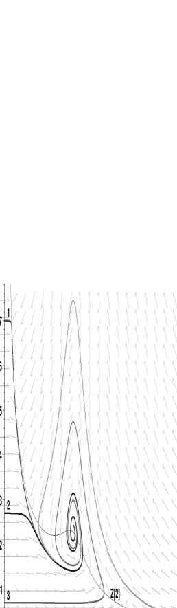
Figure 5:   The phase portrait of Eq. (25). The thin line shows the zero line Z[2] of the denominator ${\cal D}$.          

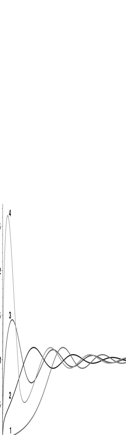
Figure 6:   The dependence of dimensionless gravitational factor g on cosmic time t for solutions of Eq. (25).          

In Fig. 4 and Fig. 5 one can see a new specific feature of 4D-DG: the solutions may enter many times the phase-space domain of inflation and the function $g(t)$ oscillates around its dSV value $\bar{g}=1$ with a variable period. Between two successive maxima of $g(t)$, the squared logarithmic derivative $H^{2}$ of $a(t)$ has its own maxima, just at the already defined time instants $t^{(i)}$. In the vicinity of each maximum of $H^{2}$, the function a(t) increases very fast – like $\exp({\rm const}\times t^{\aleph})$, with ${\rm const}>0$, and parameter $\aleph\geq 2$. Therefore, we call such inflation, which is much faster than the usual exponential de Sitter inflation, a hyper-inflation. Hence, in 4D-DG, we have some sort of successive hyper-inflations in the Universe. For simplicity, we define the time-duration $\Delta t_{infl}^{(i)}=t^{(i)}-t^{(i-1)}$, $i=0,1,...$ (by definition $\Delta t_{infl}^{(0)}=t^{(0)}$) of each of these periods of hyper-inflation as the time period between two successive dSV values of the function $g(t)$, although the hyper-inflation itself takes place only around the maxima of the function $H^{2}(t)$. The corresponding number of e-folds is ${\cal N}_{infl}^{(i)}$. It is clear that ${\cal N}_{infl}^{(i)}$ is a decreasing function of the number $i$. The inflation can be considered as cosmologically significant only if for some short total time period $\Delta t_{infl}^{total}=\sum_{i=0}^{i_{max}}\Delta t_{infl}^{(i)}$, the total number of e-folds ${\cal N}_{infl}^{total}=\sum_{i=0}^{i_{max}}{\cal N}_{infl}^{(i)}$ exceeds some large enough number ${\cal N}$. It is known that one needs to have ${\cal N}\gtrsim 60$ to be able to explain the special-flatness problem, the horizon problem, and the large-scales-smoothness problem in cosmology C .

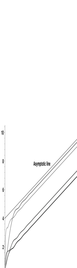
Figure 7:   The dependence of the number of e-folds ${\cal N}$ on the cosmic time $t$ for solutions of Eq. (25). The straight line gives an example of an asymptotic line for some solution.          

Fig. 7 illustrates both the inflation and the asymptotic behavior of the function ${\cal N}(t)$ for $t\to\infty$. The small oscillations of this function are “averaged” by the crude graphical abilities of the drawing device, and for large values of time $t$ we actually can see in Fig. 7 only the limiting de Sitter regime (19), when the averaged function $\langle{\cal N}(t)\rangle\equiv\langle\Delta{\cal N}(t)\rangle$. In this regime, for $t\to\infty$, we have an obvious asymptote of the form  $\langle{\cal N}(t)\rangle\sim\bar{\cal N}+\bar{H}t$ for the averaged with respect to the dilatonic oscillation (21) function $\langle{\cal N}(t)\rangle$. We accept the constant $\bar{\cal N}$ as our final definition of total number of e-folds during inflation:

$$\bar{\cal N}=\lim_{t\to\infty}\left(\langle{\cal N}(t)\rangle-\bar{H}t\right)=\lim_{t\to\infty}\left(\langle\Delta{\cal N}(t)\rangle-\bar{H}t\right).\,\,$$ (35)

It is clear that this integral characteristic describes precisely the number of e-folds due to the true inflation in the 4D-DG-RW model, i.e., during the fast initial expansion of the Universe, as a new physical phenomenon. To obtain this quantity, one obviously must subtract the asymptotic de Sitter expansion from the total function $\langle{\cal N}(t)\rangle$. It can be shown that one has to apply the same definition to the solutions in the general case of arbitrary values of the space-curvature parameter $k$ and physically admissible matter energy densities $\epsilon(a)$, since they have the same asymptotic behavior. Hence, in all cases the solutions with a cosmologically significant inflation must have values $\bar{\cal N}\gtrsim 60$.

As we see in Fig. 7, the total number of e-folds $\bar{\cal N}$ decreases, starting from the solution “4” (with $z_{0}=0.2$) to the solution “3” (with $z_{0}=0.7$) and to the solution “2” (with $z_{0}=2.7$), reaches a minimum ($\approx 1$) for some initial value $z_{0}^{*}$, and then increases for the solution “1” (with $z_{0}=7$), and for solutions with larger values of $z_{0}$. Thus, we see that inflation is a typical behavior for all solutions of Eq. (25), and that most of them have large values of $\bar{\cal N}$. (In Fig. 7, we show only solutions with small values of $\bar{\cal N}$ that are close to its minima.)

The value of the constant $\bar{\cal N}$ depends on the closeness of the given solution to the zero curve $Z[2]$ of the denominator of the integrand in the right-hand side of (16). The equation ${\cal D}=0$ can be explicitly solved. Its solution reads $z=\left({\frac{1}{3}}g^{5}u(g)\right)^{-1/4}$. The corresponding curve is shown both in Fig. 4 and Fig. 5.

The value of the quantity ${\cal N}(t)$ increases essentially each time when the solution approaches this curve. The corresponding increment of ${\cal N}(t)$ remains finite, even if the solution crosses this curve, although in this case the denominator in the integrals (16), or (34), reaches a zero value.

Indeed, taking into account that the points where the solution crosses the curve $Z[2]$ are extreme points of the function $g(z)$, and using the expansion $\Delta z=\left(-{\frac{3}{8}}z{\frac{gv{,_{g}}}{u}}\Delta g\right)^{1/2}+{\cal O}_{1}(\Delta g)$ in a vicinity of such a point, we easily obtain

$$\Delta{\cal N}=z^{-4}g^{-6}u^{-1}\sqrt{-{\frac{6u}{gv{,_{g}}}}\Delta g}+{\cal O}_{1}(\Delta g),$$

$$\Delta t={\frac{4p_{{}_{\Phi}}}{\sqrt{3}}}z^{-2}g^{-4}u^{-1}\sqrt{-{\frac{6u}{gv{,_{g}}}}\Delta g}+{\cal O}_{1}(\Delta g)$$ (36)

for potentials $u(g)$ and $v(g)$ of the most general type. Here the values of the coefficients are taken on the curve ${\cal D}=0$.

Combined with the previous results, this proves that the time intervals of inflation $t_{infl}^{(i)}$ are finite for all values of $i=0,1,\ldots$.

Thus we see that an essential increase in ${\cal N}(t)$ is accumulated when the solution becomes close and parallel to the curve $Z[2]$. This is possible both for big values of $g$ and small values of $z$ (the solution “4”), or for small values of $g$ and big values of $z$ (the solution “1”). All this results in a big value of $\bar{\cal N}$. Only a small fraction of the solutions (like the solutions “2” and “3”) stay all the time relatively far from the line ${\cal D}=0$, and therefore acquire relatively small number of e-folds, $1\lesssim\bar{\cal N}\lesssim 2-3$.

Figure 8:   The dependence of the number of e-folds $\bar{\cal N}$ on the initial value $z_{0}$ of the solutions of Eq. (25).          

The dependence of the number of e-folds on the initial value $z_{0}$ is shown in Fig. 8. Here one can see that the most of the solutions of Eq. (18) have big values of $\bar{\cal N}$. One can reach $\bar{\cal N}\sim 50-100$ for $z_{0}\sim 10-15$, i.e., without any fine tuning. An approximate form of this dependence (at a few percent level of accuracy) for $p_{{}_{\Phi}}=1/250$ is given by the following expression, obtained by a numerical analysis of the solutions of Eq. (18):

$$\bar{\cal N}(z_{0})\approx 2.552\,z_{0}^{-3/10}+0.090\,z_{0}^{8/3}.$$ (37)

Another important numerical observation is the dependence of the relation $\bar{\cal N}(z_{0},p_{{}_{\Phi}})$ on the value of the parameter $p_{{}_{\Phi}}$. As seen in Fig. 9, there is a good convergence of the corresponding family of curves, when $p_{{}_{\Phi}}\to 0$. Having in mind that in the realistic case $p_{{}_{\Phi}}\leq 10^{-30}$, we see that the inflation in 4D-DG is a robust property with respect to variations of the mass of the dilaton. The position of the minimum of the number of e-folds is at $z_{0}\approx 1.6$ and seems to be independent on this mass. The value of the minimum is $\gtrapprox 2.5$ in the limiting case $p_{{}_{\Phi}}\to 0$.

Figure 9:   The dependence of the number of e-folds $\bar{\cal N}$ on the initial value $z_{0}$ of the solutions of Eq. (25). The curves for different values $p_{{}_{\Phi}}=1/50,1/100,1/150,1/200,\,\hbox{and}\,\,\,1/250$ are shown. As seen in Fig.9, for $p_{{}_{\Phi}}\to 0$ the family of curves converges to a limiting curve, which bounds this family from above.          

This qualitative consideration, combined with the structure of the phase portrait shown in Figures 4 and 5, not only explains the universal character of the inflation in 4D-DG, but gives us a better understanding of its basic characteristics. In particular, we see that we do not need fine tuning of the model to describe the inflation as a typical physical phenomenon.

Using Eqs. (16), (17), and (26), we obtain

$${\cal N}_{infl}^{(i)}(p_{{}_{\Phi}}^{2})={\cal N}_{infl}^{(i)}(0)+{\cal O}(p_{{}_{\Phi}}^{2}),\hskip 5.69046pt$$

$$t_{infl}^{(i)}(p_{{}_{\Phi}})={\frac{4}{\sqrt{3}}}p_{{}_{\Phi}}\Theta_{infl}^{(i)}(0)+{\cal O}(p_{{}_{\Phi}}^{3}),$$

where

$${\cal N}_{infl}^{(i)}(0)=\int_{{\cal C}_{in}^{fin}(i)}\limits{\frac{dg/g}{{\cal D}(g,z;0)}},\,\,\,\hbox{and}$$

$$\Theta_{infl}^{(i)}(0)=\int_{{\cal C}_{in}^{fin}(i)}\limits{\frac{z^{2}g\,dg}{{\cal D}(g,z;0)}},\hskip 4.26773pt$$ (38)

are independent of the parameter $p_{{}_{\Phi}}$. Taking into account the extremely small physical value of this parameter, one can conclude that the higher order terms in ${\cal N}_{infl}^{(i)}(p_{{}_{\Phi}}^{2})$ and $\Delta t_{infl}^{(i)}(p_{{}_{\Phi}})$ are not essential. Neglecting them, we actually ignore the contribution of the term $\Phi/3$ in the functions $Z_{1,2}$ (8), or the corresponding term $\Phi^{2}$, in the cosmological potential $U(\Phi)$ (2). It is natural to ignore these terms in the domain of inflation, because they are essential only in a small vicinity of dSV. In the function $W(\Phi)$, we have a term that dominates for $\Phi-1\gg p_{{}_{\Phi}}^{2}$, having a huge coefficient $\sim p_{{}_{\Phi}}^{-2}$. Physically this approximation means that we are neglecting the small pure cosmological constant term in the cosmological potential and preserve only the terms, which are proportional to the mass of the dilaton.

The relation $\Delta t_{infl}^{(i)}(p_{{}_{\Phi}}^{2})\sim{\frac{4}{\sqrt{3}}}p_{{}_{\Phi}}\Theta_{infl}^{(i)}$, written in physical units, reads

$$E_{{}_{\Phi}}\Delta t_{infl}^{(i)}\sim\hbar{\frac{4}{\sqrt{3}}}\Theta_{\cal N}^{(i)}(0).$$ (39)

It resembles some kind of a quantum “uncertainty relation” for the rest energy $E_{{}_{\Phi}}$ of the dilaton and the time of inflation and probably indicates the quantum character of the inflation as a physical phenomenon.

More important for us is the fact that Eq. (39) shows the relationship between the mass of the dilaton, $m_{{}_{\Phi}}$, and the time duration of the inflation. Having large enough mass of the dilaton, we will have small time duration of the inflation. This recovers the real meaning of the mass $m_{{}_{\Phi}}$ as a physical parameter in 4D-DG, and gives possibility to determine it from astrophysical observations as a basic cosmological parameter.

V Concluding Remarks

In this section, we discuss some open problems in 4D-DG.

The main open physical problem at the moment seems to be the precise determination of the dilaton mass. The known restriction on it is too weak. It is convenient to have a dilaton $\Phi$ with mass $m_{{}_{\Phi}}$ in the range $10^{-3}$–$10^{-1}\,{\rm eV}$. In this case, the dilaton will not be able to decay into the other particles of the Standard Model, since they would have greater masses E-F_P . On the other hand, in 4D-DG we do not need such a suppressing mechanism since a direct interaction of the dilaton $\Phi$ with matter of any kind is forbidden by the weak equivalence principle F02 . This gives us the freedom to enlarge significantly the mass of the dilaton without contradiction with the known physical experiments. One of the important conclusions of the present article is that $m_{{}_{\Phi}}$ is related to the time duration of the inflation. One is tempted to try a new speculation – to investigate a 4D-DG with dilaton mass, $m_{{}_{\Phi}}$, in the domain $100\,{\rm GeV}$–$1\,{\rm TeV}$, and dilaton Compton wave length, $l_{{}_{\Phi}}$, between $10^{-18}$ and $10^{-16}\,{\rm cm}$. In this case the time-duration of the inflation, $t_{{}_{\Phi}}$, will be of order of $10^{-28}\,{\rm sec}$; the dimensionless dilaton parameter, $p_{{}_{\Phi}}$, will be about $10^{-45}$, and the ultra-high frequency, $\omega_{{}_{\Phi}}$, of dilatonic oscillations during de Sitter asymptotic regime will be approximately $10^{19}\,{\rm GHz}$. Such new values of the basic dilaton parameters are very far from the Planck scales. They seem to be accessible for the particle accelerators in the near future, and raise new physical problems.

Another open problem is the justification of quantum corrections and the exact form of cosmological potential. More general potentials than (2) where introduced in F02 , and further justification and verification is needed. One must take into account the possible additional corrections in order to obtain a correct physical description in the early Universe.

Important open problems in the development of a general theoretical framework of 4D-DG are the detailed theory of cosmological perturbations, structure formation, and possible consequences of our model for the CMB parameters. The properties of the solutions of the basic equation for linear perturbations $\delta\Phi$ differ essentially from the ones in other cosmological models with one scalar field. This equation yields a strong “clusterization” of the dilaton $\Phi$ at very small distances E-F_P . Actually, the equation for dilaton perturbations shows the existence of ultra-high frequency oscillations, described above, and non-stationary gravi-dilaton waves with length $l_{{}_{\Phi}}\leq 10^{-2}\,{\rm cm}$. Such new phenomena cannot be viewed as a clusterization at astrophysical scales. Thus, their investigation as unusual cosmological perturbations is an independent interesting issue. For example, it is interesting to know whether it is possible to consider these space-time oscillations as a kind of dark matter in the Universe.

A more profound description of the inflation in 4D-DG, both in the absence and in the presence of matter and space-curvature, is needed. It requires correct averaging of dilatonic oscillations.

We intend to present the corresponding results elsewhere.