“Observables” in causal set cosmology

Graham Brightwell , H. Fay Dowker , Raquel S. García , Joe Henson , Rafael D. Sorkin 

In memory of Sonia Stanciu

The “generic” family of classical sequential growth dynamics for causal sets [1] provides cosmological models of causal sets which are a testing ground for ideas about the, as yet unknown, quantum theory. In particular we can investigate how general covariance manifests itself and address the problem of identifying and interpreting covariant “observables” in quantum gravity. The problem becomes, in this setting, that of identifying measurable covariant collections of causal sets, to each of which corresponds the question: “Does the causal set that occurs belong to this collection?” It has for answer the probability measure of the collection. Answerable covariant questions, then, correspond to measurable collections of causal sets which are independent of the labelings of the causal sets. However, what the transition probabilities of the classical sequential growth dynamics provide directly is a measure on the space of labeled causal sets and the physical interpretation of the covariant measurable collections is consequently obscured. We show that there is a physically meaningful characterisation of the class of measurable covariant sets as unions and differences of “stem sets”.

1 Introduction

What are the observables for quantum gravity? The question is often posed but its meaning is clouded by a number of difficulties. One problem is that we do not even know what the observables are in a theory as familiar as flat spacetime non-abelian gauge theory [2]. Another major problem is that the word “observable” is inherited from an interpretation of quantum mechanics — the standard interpretation — in which the subject matter of the theory is not what $\it is$ but what can be $\it observed$. However adequate this may be for laboratory science, it will not do for quantum gravity, and we should rather be seeking what Bell called the “be-ables”. Furthermore, the question is intimately tied to the issue of general covariance, and indeed to the meaning of general covariance itself. It seems that the requirement of general covariance threatens to obscure the physical interpretation of the theory since objects identified mathematically as “covariant” may not look like anything useful for making predictions.

One advantage of the causal set approach to quantum gravity [3, 4, 5] is that it is straightforward enough conceptually that we can address these knotty problems in a productive way. Although we do not yet have a quantum dynamics for causal sets we do have a family of classical stochastic dynamics [1] within which we can investigate issues such as general covariance and the identification of observables completely concretely. The discreteness of causal sets turns out to eliminate many of the technical difficulties that tend to obscure these issues in the continuum. The work described in the current paper is a continuation of that reported in [6], and the main result is a proof of a conjecture made in that paper.

In the next section we summarise the classical sequential growth dynamics for causal sets. In the context of this dynamics, the question we started with, “What are the observables?” is replaced by, “What are the physical questions to which the dynamics provides answers?”. We see that the dynamics provides a probability measure $\mu$ on the sample space of all labeled causal sets as possible histories of the universe (these are cosmological models). Questions that we may ask are of the form: “Does the causal set that actually occurs — i.e. the real one — belong to subset $A$ of the sample space?” where $A$ is a $\mu$-measurable set, and the measure $\mu$ provides the answer: “Yes, with probability $\mu(A)$.” To be generally covariant, the questions, i.e. the subsets of the set of all labeled causal sets, must be independent of labeling. Thus we are led to the identification of the covariant questions as subsets $A$ of the set of all causal sets such that if a certain labeled causal set is an element of $A$, so are all its re-labelings.

This identification is, however, very abstract and what we are seeking, then, is a characterisation of the measurable sets that will be physically useful. In section 3 we describe the result that we will prove, namely that any measurable set of causal sets can be formed by countable set operations on the so-called “stem sets,” to be defined. These stem sets have an accessible physical meaning. Sections 4, 5 and 6 are devoted to proving the theorem and the last section contains a discussion.

2 Classical sequential growth models and the covariant questions

The causal set hypothesis is that the continuum spacetime of general relativity is an approximation to a deeper level of discrete structure which is a past finite partial order or causal set (causet). This is a set endowed with a binary relation $\prec$ such that $(x\prec y)\,{\rm and}\,(y\prec z)\implies(x\prec z)$ (transitivity), $x\not\prec x$ (acyclicity), and all “past-sets” $\left\{x\,|\,x\preceq z\right\}$ are finite. (The condition that all past-sets are finite implies that the partial order is locally finite. In other contexts one would weaken the condition of past finiteness to local finiteness in the definition of a causet, but for present purposes there is no harm in using the stronger condition.) When $x\prec y$ we say that “$x$ is below $y$” or “$y$ is above $x$.” We will be interested in both finite and countably infinite causets.

Although we don’t yet have a quantum dynamics for causal sets, the generic family of classical sequential growth (CSG) dynamics derived in [1] is a good place to begin the search for physical questions, as a warm-up for the quantum theory when we have it.

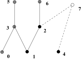
Figure 1: Transition from stage 7 to stage 8 of a particular growth process. Two vertices joined by a line are related, with the lower being to the past of (an ancestor of) the upper one. Only covering relations (“links”) are represented, the rest being implied by transitivity. Points filled with black are to the past of the new element (8) and points filled with grey are spacelike to it.

Each of the dynamical laws in question describes a stochastic birth process in which elements are “born” one by one so that, at stage $n$, it has produced a causet $\tilde{c}_{n}$ of $n$ elements, within which the most recently born element is maximal. If one employs a genealogical language in which “$x\prec{y}$” can be read as “$x$ is an ancestor of $y$”, then the $n^{th}$ element (counting from $0$) must at birth “choose” its ancestors from the elements of $\tilde{c}_{n}$, and for consistency it must choose a subset $s$ with the property that $x\prec{y}\in{s}{\,\implies\,}x{\in}s$. (Every ancestor of one of my ancestors is also my ancestor.) Such a subset $s$ (which is necessarily finite) will be called a stem. The dynamics is then determined fully by giving the transition probabilities governing each such choice of $s\subset\tilde{c}_{n}$.

We can formalize this scheme by introducing for each integer $n=0,1,2,\cdots$ the set $\tilde{\Omega}(n)$ of labeled causets $\tilde{c}_{n}$ whose elements are labeled by integers $0,1,\cdots,n-1$ that record their order of birth. Moreover this labeling $L$ is natural in the sense that $x{\prec}y{\,\implies\,}L(x)<L(y)$. Each birth of a new element occasions one of the allowed transitions from $\tilde{\Omega}(n)$ to $\tilde{\Omega}(n+1)$ and occurs with a specified conditional probability $\tau$.

A specific stochastic dynamics is fixed by giving the $\tau$ for all possible transitions. Under the physically motivated assumptions of “discrete general covariance” and “Bell Causality” the possibilities for the $\tau$ are severely narrowed down and have been largely classified in [1]. The main conclusion is that $\tau$ generically takes the form

$$\tau=\frac{\lambda(\varpi,m)}{\lambda(n,0)}$$ (1)

where, for the potential transition in question, $\varpi$ is the number of ancestors of the new element, $m$ the number of its “parents”, and $n$ the number of elements present before the birth, and where $\lambda(\varpi,m)$ is given by the formula $\sum_{k}{\varpi-m\choose k-m}t_{k}$ with the non-negative real numbers $t_{k}$ being the free parameters or “coupling constants” of the theory.

An alternative intepretation of this dynamical rule is as follows. Each new element chooses some set $s$ of elements from among those already present, a set $s$ being chosen with relative probability $t_{|s|}$: then the new element is placed above $s$ and all ancestors of members of $s$. Setting $t_{k}=t^{k}$, where $t$ is constant, gives the model of “random graph orders” as studied in [7], [8], [9] and [10], for instance. In [1] this special case was called “percolation”. One can thus understand the dynamical rule given by (1) as defining a type of “generalized percolation model”. These models exhaust the “generic” solution family of [1], and they are the only ones we consider in this paper. (We thereby ignore such “exceptional” CSG models as “originary percolation”, not to mention those exceptional solutions which are not even limits of the generalized percolation form.)

There are two simple cases that we can describe completely: if all the $t_{k}$ are zero except $t_{0}$, then we obtain a causet in which no pair of elements is related, while if only $t_{0}$ and $t_{1}$ are non-zero we almost surely obtain a causet which is an infinite union of trees in which every element has infinitely many children. For the present, we rule out these two cases, so we assume that $t_{k}>0$ for some $k\geq 2$, but we do not need to make any other assumptions regarding the coupling constants in the model.

The stochastic dynamics described above gives rise to a notion of probability that is too rich for our purposes, as it assigns a probability as an answer to the question “is element 3 above element 1?”, which is not meaningful for us, as in any particular causet the answer depends on the labeling of the elements. In order to arrive at a definite theory one needs to specify the set of questions that the theory should answer and for each one of them, explain how in principle, the probability of the answer “yes” can be computed.

We will need to proceed in a formal manner. We wish to construct a probability space, which is a triad consisting of: a sample space $\Omega$, a $\sigma$-algebra $\mathcal{R}$ on $\Omega$, and a probability measure $\mu$ with domain $\mathcal{R}$. In relation to the two tasks above, each member $Q$ of $\mathcal{R}$ corresponds to one of the answerable questions and its measure $p=\mu(Q)$ is the answer. (That $\mathcal{R}$ is a $\sigma$-algebra on $\Omega$ means that it is a non-empty family of subsets of $\Omega$ closed under complementation and countable intersection. A probability measure $\mu$ with domain $\mathcal{R}$ is a function that assigns to each member of $\mathcal{R}$ a non-negative real number — its probability — such that $\mu$ is countably additive, with $\mu(\Omega)=1$. Finally, countable additivity means that $\mu(\cup_{n}A_{n})=\sum_{n}\mu(A_{n})$ for any countable collection of mutually disjoint sets in $\mathcal{R}$.)

In the case at hand, the sample space is the set $\tilde{\Omega}\equiv\tilde{\Omega}(\infty)$ of completed labeled causets, these being the infinite causets that would result if the birth process were made to “run to completion”. (We use a tilde to indicate labeling.) The dynamics is then given by a probability measure $\tilde{\mu}$, constructed from the transition probabilities $\tau$, whose domain $\tilde{\mathcal{R}}$ is a $\sigma$-algebra specified as follows. To each finite causet $\tilde{b}\in\tilde{\Omega}(n)$ one can associate the “cylinder set” ${\rm cyl}(\tilde{b})$ comprising all those $\tilde{c}\in\tilde{\Omega}$ whose first $n$ elements (those labeled $0\cdots{n-1}$) form an isomorphic copy of $\tilde{b}$ (with the same labeling); and $\tilde{\mathcal{R}}$ is then the smallest $\sigma$-algebra containing all these cylinder sets. More constructively, $\tilde{\mathcal{R}}$ is the collection of all subsets of $\tilde{\Omega}$ which can be built up from the cylinder sets by a countable process involving countable union, intersection and complementation. The transition probabilities $\tau$ provide us with the probability of each cylinder set ${\rm cyl}(\tilde{b})$, and standard results in probability theory imply that this extends to a probability measure on $\tilde{\mathcal{R}}$.

For future use, we will need in addition to $\tilde{\Omega}$ the corresponding space $\Omega$ of completed unlabeled causets, whose members can also be viewed in an obvious manner as equivalence classes within $\tilde{\Omega}$. We will also need the set of all finite labeled causets $\tilde{\Omega}(\mathbb{N})\equiv\cup_{n\in\mathbb{N}}\tilde{\Omega}(n)$ and its unlabeled counterpart $\Omega(\mathbb{N})=\cup_{n\in\mathbb{N}}\Omega(n)$.

At first hearing, calling a probability measure a dynamical law might sound strange, but in fact, once we have the measure $\tilde{\mu}$ we can say everything of a predictive nature that it is possible to say a priori about the behavior of the causet $\tilde{c}$. For example, one might ask “Will the universe recollapse?” This can be interpreted mathematically as asking whether $\tilde{c}$ will develop a “post”, defined as an element whose ancestors and descendants taken together exhaust the remainder of $\tilde{c}$. Let $A\subset\tilde{\Omega}$ be the set of all completed labeled causets having posts. (One can show that $A\in\tilde{\mathcal{R}}$, so that $\tilde{\mu}(A)$ is defined.) Then our question is equivalent to asking whether $\tilde{c}\in{A}$, and the answer is “yes with probability $\tilde{\mu}(A)$.” It is thus $\tilde{\mu}$ that expresses the “laws of motion” (or better “laws of growth”) that constitute our stochastic dynamics: its domain $\tilde{\mathcal{R}}$ tells us which questions the laws can answer, and its values $\tilde{\mu}(A)$ tell us what the answers are.

In this context, we can see what the expression of general covariance is. In a causet, only the relations between elements have physical significance: the labels on causet elements are considered as physically meaningless. Thus, for a subset of $A\subset\tilde{\Omega}$ to be covariant, it cannot contain any labeled completed causet $\tilde{c}$ without containing at the same time all those $\tilde{c}^{\prime}$ isomorphic to $\tilde{c}$ (i.e. differing only in their labelings). To be measurable as well as covariant, $A$ must also belong to $\tilde{\mathcal{R}}$. Let $\mathcal{R}$ be the collection of all such sets: $A\in\mathcal{R}{\iff}{A}\in\tilde{\mathcal{R}}\ {\rm and}\ \forall\tilde{c}_{1}\simeq\tilde{c}_{2}\in\tilde{\Omega},\tilde{c}_{1}\in{A}\implies\tilde{c}_{2}\in{A}$. It is not hard to see that $\mathcal{R}$ is a sub-$\sigma$-algebra of $\tilde{\mathcal{R}}$, whence the restriction of $\tilde{\mu}$ to $\mathcal{R}$ is a measure $\mu$ on the space $\Omega$ of unlabeled completed causets. (As just defined, an element $A\in\mathcal{R}$ is a subset of $\tilde{\Omega}$. However, because it is re-labeling invariant, it can also be regarded as a subset of $\Omega$.) Any element of $\mathcal{R}$ corresponds to a covariant question to which the dynamics provides the answer in the form of $\mu$.

However, the definition of $\mathcal{R}$ provides no useful information about the physical meaning of these covariant questions. All we know is that an element of $\mathcal{R}$ is formed from the (non-covariant) cylinder sets by doing countably many set operations after which the resulting set must contain all re-labelings of each of its elements. Our purpose now is to provide a construction of $\mathcal{R}$ that is physically useful.

3 The physical questions

Among the questions belonging to $\mathcal{R}$ there are some which do have a clear significance. Let $b\in\Omega(\mathbb{N})$ be a finite unlabeled causet and let ${\rm{stem}}(b)\subset\Omega$ be the “stem set”, ${\rm{stem}}(b)=\left\{c\in\Omega\,|\,c\mbox{ contains a stem isomorphic to }b\right\}$. Thus ${\rm{stem}}(b)$ comprises those unlabeled completed causets with the property that there exists a natural labeling such that the first $n$ elements form a causet isomorphic to $b$. Each stem set ${\rm{stem}}(b)$ — treated as a subset of $\tilde{\Omega}$ — is a countable union of cylinder sets:

$${\rm{stem}}(b)=\bigcup\left\{{\rm cyl}(\tilde{c})\,|\,\tilde{c}\in\Omega({\hbox{\openface N}})\mbox{ and }b\mbox{ is a stem in }\tilde{c}\right\}$$

Therefore the stem sets belong to $\tilde{\mathcal{R}}$ and hence to $\mathcal{R}$. For this particular element of $\mathcal{R}$, the meaning of the corresponding causet question is evident: “Does the causet contain $b$ as a stem?”.

Note on terminology: strictly, “$a$ is a stem in $c$” and “$c$ contains $a$ as a stem” mean that $a$ is a subset of $c$. We will often abuse this terminology and say “$a$ is a stem in $c$” when we mean that $c$ contains a stem isomorphic to $a$. The context should ensure that no confusion arises. For example, we say that causets $a$ and $b$ “have the same stems” when any $d\in\Omega(\mathbb{N})$ is a stem in $a$ if and only if it is a stem in $b$.

Equally evident is the significance of any question built up as a logical combination of stem questions of this sort. To such compound stem questions belong members of $\mathcal{R}$ built up from stem sets ${\rm{stem}}(b)$ using union, intersection and complementation (corresponding to the logical operators ‘or’, ‘and’ and ‘not’, respectively). If all the members of $\mathcal{R}$ were of this type, we would not only have succeeded in characterizing the dynamically meaningful covariant questions at a formal level, but we would have understood their physical significance as well. The following theorem asserts that, to all intents and purposes, this is the case.

Theorem 1

For every CSG dynamics as described in section 2, the family $\cal{S}$ of all stem sets generates the $\sigma$-algebra $\mathcal{R}$ up to sets of measure zero.

This is a little vague so let us work towards formulating a more precise statement. Let $\cal{R}({\cal{S}})$ be the $\sigma$-algebra generated by $\cal{S}$. Since $\cal{S}\subset\cal{R}$ we know that $\cal{R}({\cal{S}})\subset\cal{R}$. Unfortunately the latter inclusion is strict: there exist sets in $\cal{R}$ which are not in $\cal{R}({\cal{S}})$. The following is an example. Let

$$\Gamma=\left\{c\in\Omega\,|\,c\mbox{ contains a maximal element}\right\}$$

and

$$\Gamma_{k}^{n}=\{\tilde{c}\in\tilde{\Omega}:\;\;e(k)\not\prec e(m)\;\;\mbox{for}\;k<m\leq n\}$$

where $e(j)$ is the element of $\tilde{c}$ labeled $j$.

This latter set is a finite union of cylinder sets, since the condition requires the initial stretch of $\tilde{c}$ to be in a particular subset of $\tilde{\Omega}(n)$, and

$$\Gamma=\overset{\infty}{\underset{k=0}{\cup}}\;\overset{\infty}{\underset{n=k\!+\!\!\,1}{\cap}}\,\Gamma_{k}^{n}$$

Therefore $\Gamma\in\tilde{\mathcal{R}}$ and, because the defining condition of $\Gamma$ is manifestly covariant, $\Gamma$ is moreover in $\mathcal{R}$ .

To show that $\Gamma\notin\mathcal{R}(\mathcal{S})$, we argue as follows. If there exist two completed causets $x,y\in\Omega$ such that every stem set $S\in\mathcal{S}$ contains either both $x$ and $y$ or neither, then the same holds for every $A\in\mathcal{R}(\mathcal{S})$. This is because

$$\mathcal{R}^{\prime}\equiv\{A\in\mathcal{R}(\mathcal{S}):\;\;\mbox{either}\;\;x,y\in A\;\;\mbox{or}\;\;x,y\in A^{c}\}$$

is a $\sigma$-algebra and $\mathcal{R}^{\prime}$ contains $\mathcal{S}$ and therefore contains $\mathcal{R}(\mathcal{S})$. Consider now the following two causets: $c_{1}$ is the union of infinitely many unrelated infinite chains (a chain is a totally ordered set) and $c_{2}$ is the union of $c_{1}$ and a single unrelated element (see figure 2). Clearly, $c_{1}\notin\Gamma$, while $c_{2}\in\Gamma$. Now $c_{1}$ and $c_{2}$ cannot be separated by sets in $\mathcal{S}$: if a finite causet is a stem in $c_{1}$ it is also a stem in $c_{2}$ and vice versa. Therefore $\Gamma$, which does separate the two, cannot be in $\mathcal{R}(\mathcal{S})$.

Figure 2: Every stem in causet 1 is also found in causet 2 and vice versa. Since they have the same stems, they cannot be separated by sets in $\mathcal{S}$ nor in $\mathcal{R}(\mathcal{S})$.

In this example, the two causets responsible for the failure of $\cal{R}$ and $\cal{R}({\cal{S}})$ to be equal have the property that they are non-isomorphic but have the same stems. This suggests that the “difference” between the two $\sigma$-algebras is due to such causets, which we call “rogue” causets. A causet $c\in\Omega$ is a rogue if there exists a non-isomorphic causet $c^{\prime}\in\Omega$ such that if $b\in\Omega(n)$ is a stem in $c$ then it is a stem in $c^{\prime}$ and vice versa. Let $\Theta$ be the set of all rogues in $\Omega$.

Now we state two propositions that will easily imply our result.

Proposition 1

$\mu(\Theta)=0$ in any CSG dynamics

Proposition 2

For every set $A\in\mathcal{R}$, there is a set $B\in\mathcal{R}(\mathcal{S})$ such that $A\triangle B\subset\Theta$.

Here $\triangle$ denotes symmetric difference.

The following immediate corollary is a precise version of Theorem 1.

Corollary 1

For every set $A\in\mathcal{R}$, there is a set $B\in\mathcal{R}(\mathcal{S})$ such that, in any CSG dynamics, $\mu(A\triangle B)=0$.

The rest of the paper is devoted to proving the two propositions.

4 Proof of Proposition 1

We begin with a little terminology. An element $x$ of a causet is maximal if there is no $y$ with $x\prec y$ and minimal if there is no $z$ with $z\prec x$. The past of an element $x$ is the set of elements below $x$. A chain of length $k$ in a causet is a sequence $x_{0}\prec\cdots\prec x_{k}$. The level of an element $x$ in a causet is the maximum length of a chain with top element $x$ — so elements at level 0 are exactly minimal elements, and those at level 1 are the non-minimal elements that are above only minimal elements. As causets are past finite, every element has some finite level. Naturally, level $k$ in a causet consists of the elements of level $k$. If $a$ is a causet, $a_{(k)}$ denotes the set of all elements of level less than or equal to $k$.

We shall actually characterize exactly the set of rogues, although this is more than we need.

Let $\Gamma=\left\{c\in\Omega\,|\,c\hbox{ has a level containing infinitely many non-maximal elements}\right\}$. Then we have

Lemma 1

$\Gamma\subset\Theta$.

Proof  Let $a\in\Gamma$. Suppose level 0 in $a$ has infinitely many non-maximal elements. If level 0 in $a$ also contains any non-zero number of maximal elements, let causet $b$ be formed from $a$ by deleting all those level 0 maximal elements. If level 0 in $a$ contains no maximal elements, let $b$ be formed by adding a maximal element to level 0. Then $a\not\simeq b$ and they have the same stems.

Now suppose that level $k$ is the first level in $a$ with infinitely many non-maximal elements, so that all levels below $k$ have finitely many non-maximal elements. As $a_{(k-1)}$, the set of elements at levels below $k$, is finite, there exist an infinite number of non-maximal elements in level $k$ of $A$ which all share the same past — a given subset $c\subset a_{(k-1)}$. If there is any non-zero number of maximal elements in level $k$ of $a$ with past $c$, then let causet $b$ be formed from $a$ by deleting all those elements. If there are no maximal elements in level $k$ of $a$ with past $c$, then let causet $b$ be formed from $a$ by adding a maximal element with past $c$. Then $a\not\simeq c$ and they have the same stems. $\Box$

Lemma 2

$\Theta\subset\Gamma$.

Proof  Consider $a\not\in\Gamma$. Suppose that $b\in\Omega$ has the same stems as $a$. We want to show that $a\simeq b$, which then implies that $a\not\in\Theta$.

The plan is to construct partial isomorphisms between $a_{(k)}$ and $b_{(k)}$ for each $k$, and then show that some subsequence of these partial isomorphisms extends to an isomorphism of the completed causet. Our task is complicated by the possible infinite sets of maximal elements at each level. We deal with these by a process that we have called “Hegelianization”.

A completed causet $a$ is Hegelianized as follows. First one defines an equivalence relation in $a$ by setting $x\sim y$ iff either $x=y$ or they are both maximal, have the same past and there are infinitely many elements with that same past. The Hegelianization of $a$ is then the quotient causet $a^{*}=a/\sim$; since $a\notin\Gamma$, all levels of $a^{*}$ are finite. To each element in $a^{*}$ that is an infinite equivalence class, we attach a flag: note that every unflagged element of $a^{*}$ is a single-element equivalence class $\{x\}$, which we naturally identify with the element $x$ of $a$.

For each $k$, we claim that there is an isomorphism between $a^{*}_{(k)}$ and $b^{*}_{(k)}$ that preserves the flags. In showing this, we may assume that the following hold:
(i) $a^{*}_{(k)}$ contains at least as many flagged elements as $b^{*}_{(k)}$,
(ii) if the two sets contain the same number of flagged elements, then $|a^{*}_{(k)}|\geq|b^{*}_{(k)}|$.
(Otherwise, exchange the roles of $a$ and $b$.)

Let $N=|b^{*}_{(k)}|+1$. Let $c$ be obtained from $a^{*}_{(k)}$ by (a) replacing each flagged element $x$ by $N$ elements $x_{1},\dots,x_{N}$, and (b) for each element $y$ of $a^{*}_{(k)}$ that is maximal in $a^{*}_{(k)}$ but not in $a$, include some element $z_{y}$ above $y$ in $a$, and also all elements in the past of $z_{y}$. So $c$ is a stem in $a$, in which all the newly introduced elements $x_{i}$ are maximal. Hence $c$ is also a stem in $b$, i.e. there is an embedding $\varphi:c\hookrightarrow b$ whose image is a stem in $b$. Note that $\varphi$ preserves levels. So, for any flagged element $x$ of $a^{*}_{(k)}$, all of $\varphi(x_{1}),\dots,\varphi(x_{N})$ are different elements of $b_{(k)}$, so by choice of $N$ at least one of them, say $\varphi(x_{1})$, is in an infinite equivalence class. If $y\in a^{*}_{(k)}$ is not maximal in $a$, then $\varphi(y)<\varphi(z_{y})$, so $\varphi(y)$ is not maximal in $b$.

We now obtain a natural map $\varphi^{*}:a^{*}_{(k)}\hookrightarrow b^{*}_{(k)}$, defined by taking each unflagged element $z\in a^{*}_{(k)}$ to the equivalence class containing $\varphi(z)$, and each flagged element $x$ to the equivalence class containing $\varphi(x_{1})$.

We claim that distinct elements $x$ and $y$ of $a^{*}_{(k)}$ are mapped to distinct elements of $b^{*}_{(k)}$ by $\varphi^{*}$. If neither $x$ nor $y$ is maximal in $a$, then this is immediate since $\varphi(x)\not=\varphi(y)$, and these elements are unflagged in $b$. If $x$ is maximal in $a$ and $y$ is not, then $\varphi^{*}(x)$ is maximal in the image of $\varphi^{*}$ while $\varphi^{*}(y)$ is not. If $x$ and $y$ are both maximal in $a$, but not in the same equivalence class, then either they have different pasts — in which case they are certainly mapped to different elements — or there are only finitely many elements with the same past as $x$ and $y$. In this last case, we have to rule out the possibility that the unflagged elements $x$ and $y$ are mapped to a flagged element of $b^{*}_{(k)}$; this is not possible, since we have shown that distinct flagged elements of $a^{*}_{(k)}$ are mapped to distinct flagged elements of $b^{*}_{(k)}$, and by assumption there are no more flagged elements of $b^{*}_{(k)}$.

This shows that $\varphi^{*}$ is an embedding of $a^{*}_{(k)}$ into $b^{*}_{(k)}$, and furthermore that the two sets have the same number of flagged elements. As $|a^{*}_{(k)}|\geq|b^{*}_{(k)}|$, the map $\varphi^{*}$ is actually an isomorphism. In particular, $|a^{*}_{(k)}|=|b^{*}_{(k)}|$ for each $k$.

Now take a sequence $(\varphi^{*}_{k})$, where $\varphi^{*}_{k}$ is an isomorphism from $a^{*}_{(k)}$ to $b^{*}_{(k)}$. We construct an isomorphism from $a^{*}$ to $b^{*}$ by a standard “compactness” procedure. Note that there are only finitely many 1-1 maps from level 0 of $a^{*}$ to level 0 of $b^{*}$; each $\varphi^{*}_{k}$ induces one of these maps, so one such map occurs infinitely often, say for all $k$ in the infinite set $K_{0}$. Similarly, there is an infinite subset $K_{1}$ of $K_{0}$ such that each $\varphi^{*}_{k}$ for $k\in K_{1}$ induces the same map from level 1 of $a^{*}$ to level 1 of $b^{*}$. We continue in this way for all levels. The isomorphism $\Phi$ is then defined by combining the 1-1 maps obtained at each level: $\Phi$ is clearly order-preserving and a bijection.

Having found an isomorphism from $a^{*}$ to $b^{*}$, it is trivial to extend it to an isomorphism from $a$ to $b$, as required. $\Box$

Corollary 2

$\Theta=\Gamma$.

Lemma 3

$\Theta$ is measurable. Indeed $\Theta\in\mathcal{R}(\mathcal{S}).$

Proof  We show that $\Gamma$ can be constructed countably from the stem sets, which are themselves measurable.

Let $\Gamma_{kl}^{n_{0}\cdots n_{k-1}}$ be defined as the union of finitely many stem sets as follows. Each stem set in the union is defined by a stem which: is a finite causet with $n_{i}$ elements in level $i,\;i=0,\cdots,k-1$, $l$ elements in level $k$ and $m\leq l$ elements in level $k+1$, ordered in such a way that all the elements in levels $i\leq k$ are non-maximal. There are only finitely many such stems and the union is over all corresponding stem sets.

Define $\Gamma_{kl}$ to be the union of these over $n_{i}$, $i=0,\cdots,k-1$ for fixed $k$ and $l$:

$$\Gamma_{kl}=\overset{\infty}{\underset{n_{k\!-\!\!\,1}=1}{\cup}}\cdots\overset{\infty}{\underset{n_{0}=1}{\cup}}\,\Gamma_{k}^{n_{0}\cdots n_{k-1}}\ .$$

This is the set of all causets with at least $l$ non-maximal points at level $k$. Then, taking the intersection over $l$ and finally the union over $k$ we see that

$$\Gamma=\,\overset{\infty}{\underset{k=0}{\cup}}\,\overset{\infty}{\underset{l=0}{\cap}}\,\Gamma_{kl}\ .$$

$\Box$

Lemma 4

In the CSG dynamics with $t_{k}\neq 0$ for some $k>1$, a causet containing an infinite level almost surely does not occur.

Proof  As we have already seen, a causet contains an infinite level if and only it if contains an infinite antichain (an antichain is a totally unordered set) all of whose elements share the same past.

Fix any labeled stem $\tilde{c}$, and let $n_{0}$ be the largest label in $\tilde{c}$; we show that there are almost surely only finitely many elements of the causet with past $\tilde{c}$. It is enough to show that the expected number of elements with past equal to $\tilde{c}$ is finite (this is exactly the Borel-Cantelli Lemma). The expected number of elements with past $\tilde{c}$ is the sum, over $n>n_{0}$, of the probability that $e(n)$, the element labeled $n$, has past $\tilde{c}$.

Recall that this probability is

$$\tau_{n}=\frac{\sum_{l=m}^{\varpi}\binom{\varpi-m}{l-m}t_{l}}{\sum_{j=0}^{n}\binom{n}{j}t_{j}}$$ (2)

where $\varpi$ is the number of elements in $\tilde{c}$ and $m$ the number of maximal elements in $\tilde{c}$. Therefore the expected number of elements with past $\tilde{c}$ is

$$\sum_{n=n_{0}+1}^{\infty}\tau_{n}=\sum_{l=m}^{\varpi}\binom{\varpi-m}{l-m}t_{l}\sum_{n=n_{0}+1}^{\infty}\frac{1}{\sum_{j=0}^{n}\binom{n}{j}t_{j}}.$$

Because there is some $j\geq 2$ with $t_{j}>0$, the terms in the last sum above are bounded above by those in the convergent series $\sum 1/\binom{n}{j}t_{j}$. Hence the sum is finite, and the expectation is finite, as required. $\Box$

Since $\Theta$ is a subset of the set of causets with an infinite level we have:

Corollary 3

$\Theta$ has measure zero.

This is our proposition 1.

5 Some results in measure theory

In order to prove proposition 2 it will be necessary to be a little more formal than we have been heretofore. In this section we collect some relevant definitions and results from measure theory. For the most part, we follow the terminology of Mackey [11].

Recall that a $\sigma$-algebra $\mathcal{R}$ on a set $X$ is a non-empty family of subsets of $X$ closed under complementation and countable union; that is, $\mathcal{R}$ must satisfy: (i) if $A\in\mathcal{R}$ then $A^{c}\in\mathcal{R}$, and (ii) if $A_{n}\in\mathcal{R}$ for every $A_{n}$ in a countable family, then $\bigcup_{n}A_{n}\in\mathcal{R}$. By a Borel space we will mean a pair $(X,\mathcal{R})$ where $X$ is a set and $\mathcal{R}$ is a $\sigma$-algebra on $X$. The members of $\mathcal{R}$ will be called measurable subsets or Borel subsets.

For any family $\mathcal{F}$ of subsets of $X$, the $\sigma$-algebra generated by $\mathcal{F}$, denoted $\mathcal{R}(\mathcal{F})$, is the smallest $\sigma$-algebra that includes every member of $\mathcal{F}$. If $\mathcal{F}$ is a family of subsets of $X$ and $A$ an arbitrary subset of $X$, we write $\mathcal{F}\cap A$ to denote the family $\left\{F\cap A\,|\,F\in\mathcal{F}\right\}$ of subsets of $A$. If $\mathcal{F}$ is a $\sigma$-algebra, then so also is $\mathcal{F}\cap A$. If $(X,\mathcal{R})$ is a Borel space and $A$ is an element of $\mathcal{R}$, then we call the pair $(A,\mathcal{R}\cap A)$ a Borel subspace of $(X,\mathcal{R})$. (We emphasize that according to this definition, only a measurable subset $A$ yields a Borel subspace.)

Given two Borel spaces $(X,\mathcal{R})$ and $(X^{\prime},\mathcal{R}^{\prime})$, a map $f:X\rightarrow X^{\prime}$ is said to be a Borel map if for each $A\in\mathcal{R}^{\prime}$, the set $f^{-1}(A)$ is in $\mathcal{R}$. For any equivalence relation in a Borel space $(X,\mathcal{R})$, a $\sigma$-algebra $\mathcal{R}^{\prime}$ is induced in the space $X^{\prime}$ of equivalence classes by requiring the projection $p:X\rightarrow X^{\prime}$ to be a Borel map. Concretely, $\mathcal{R}^{\prime}$ is the family of subsets $A^{\prime}\subset X^{\prime}$ such that $p^{-1}(A^{\prime})\in\mathcal{R}$. The derived Borel space $(X^{\prime},\mathcal{R}^{\prime})$ is called a quotient of $(X,\mathcal{R})$. A quotient of a Borel subspace of a Borel space $(X,\mathcal{R})$ is called a Borel subquotient of $(X,\mathcal{R})$.

Lemma 5

Let $A\subset X$ be a measurable subset in the Borel space $(X,\mathcal{R})$. Then $\mathcal{R}(\mathcal{F}\cap A)=\mathcal{R}(\mathcal{F})\cap A$.

This is intuitively obvious because intersecting with $A$ preserves complement and countable union. A proof is given in [12], page 132.

A family $\mathcal{F}$ of measurable subsets of $X$ is said to separate a Borel space $(X,\mathcal{R})$ (or to be a separating family for $(X,\mathcal{R})$) if for every two points $x$, $y\in X$, there exists a set $U\in\mathcal{F}$ with $x\in U$ and $y\notin U$.

Naturally associated with any topological space $X$, is the $\sigma$-algebra generated by the family of open (or equivalently closed) subsets of $X$. This is called the topological $\sigma$-algebra of $X$.

A topological space $X$ is separable if it contains a countable dense subset $D$. (When $X$ is a metric space, this signifies that every open ball in $X$ contains a point of $D$.) A Polish space is a separable complete metric space.

We are now in a position to state a key theorem we will use in proving Proposition 2.

Theorem 2

In a Borel subquotient of a Polish space, any countable separating family is also a generating family.

Proof  Combine the second theorem on page 74 of [11] with the corollary on page 73, bearing in mind the definition of a standard Borel space as a Borel subspace of a Polish space. $\Box$

6 Proof of Proposition 2

We now place the spaces and measures of our causal set stochastic process within this formal framework. Let $\mathcal{C}$ be the family of cylinder sets in $\tilde{\Omega}$. It is countable, since its members are in one-to-one correspondence with the collection of finite labeled causets. Each particular choice of CSG dynamics assigns a probability to each set in $\mathcal{C}$. Standard techniques then assure us that this assignment extends in a unique way to a probability measure $\tilde{\mu}$ in the Borel space $(\tilde{\Omega},\tilde{\mathcal{R}})$, where as before $\tilde{\mathcal{R}}=\mathcal{R}(\mathcal{C})$ is the $\sigma$-algebra generated by $\mathcal{C}$.

Lemma 6

There is a metric on $\tilde{\Omega}$ with respect to which $\tilde{\Omega}$ is a Polish space whose topological $\sigma$-algebra is $\tilde{\mathcal{R}}$.

Proof  For each pair of completed labeled causets $\tilde{a}$, $\tilde{b}\in\tilde{\Omega}$, we set:

$$d(\tilde{a},\tilde{b})=1/2^{n},$$ (3)

where $n$ is the largest integer for which $\tilde{a}_{(n)}=\tilde{b}_{(n)}$. It is easy to verify that this gives a metric on $\tilde{\Omega}$. The maximum distance between two causets is $1/2$ and occurs when their initial two elements already form distinct partial orders. Note also that the open balls in this metric are exactly the cylinder sets.

One can readily verify that the metric space $(\tilde{\Omega},d)$ given by (3) is complete. To see that it is separable we find a countable dense set in $\tilde{\Omega}$. Associate with each finite causet $\tilde{a}\in\tilde{\Omega}(n)$, the completed causet which results from adding an infinite chain to the future of the last element in $\tilde{a}$. It is then clear that for any causet $\tilde{c}\in\tilde{\Omega}$ such a ‘chain-tailed’ causet can be found arbitrarily close to $\tilde{c}$. Therefore $\tilde{\Omega}$ is a Polish space with respect to the metric $d$.

The family of open balls about the points in this countable dense set is exactly the family of cylinder sets, and therefore the topological $\sigma$-algebra coincides with $\tilde{\mathcal{R}}$, as required. $\Box$

Recall that we have defined $\mathcal{R}$ as the subalgebra of all label-invariant Borel sets in $\tilde{\mathcal{R}}$ and that one can also think of $\mathcal{R}$ as a $\sigma$-algebra in the space of unlabeled causets $\Omega$.

Consider the equivalence relation of isomorphism on the set $\tilde{\Omega}$ of labeled causets. The set of equivalence classes is in 1-1 correspondence with the set $\Omega$ of unlabeled completed causets. Let $p:\tilde{\Omega}\rightarrow\Omega$ be the projection, which assigns to each labeled causet $\tilde{c}$ the class $[\tilde{c}]$ of all its possible labelings, corresponding to the unlabeled causet $c$. Sets of the form $p^{-1}(A)$ are label-invariant subsets of $\tilde{\Omega}$; to say that this set is in $\tilde{\mathcal{R}}$ (or in $\mathcal{R}$) is equivalent to saying that the corresponding set $A$ of unlabeled causets is in $\mathcal{R}$. Therefore $(\Omega,\mathcal{R})$ is a quotient of $(\tilde{\Omega},\tilde{\mathcal{R}})$.

Furthermore the measure $\tilde{\mu}$ on $(\tilde{\Omega},\tilde{\mathcal{R}})$ restricts to a measure $\mu$ on $\mathcal{R}$, which we can define within either interpretation of $\mathcal{R}$. Viewing $\mathcal{R}$ as a subalgebra of $\tilde{\mathcal{R}}$ in $\tilde{\Omega}$, we have $\mu=\tilde{\mu}_{|\mathcal{R}}$. While viewing $\mathcal{R}$ as the quotient of $\tilde{\mathcal{R}}$ in $\Omega$, we have $\mu=\tilde{\mu}\circ p^{-1}$.

Define $\tilde{\Omega}_{0}=\tilde{\Omega}\setminus\tilde{\Theta}$ and let $\tilde{\mathcal{R}}_{0}=\tilde{\mathcal{R}}\cap\tilde{\Omega}_{0}$ be the induced $\sigma$-algebra in $\tilde{\Omega}_{0}$. Then $(\tilde{\Omega}_{0},\tilde{\mathcal{R}}_{0})$ is a Borel subspace of $(\tilde{\Omega},\tilde{\mathcal{R}})$ (it follows from Lemma 3 that $\tilde{\Omega}_{0}$ is a Borel subset of $\tilde{\Omega}$). Similarly let $\Omega_{0}=\Omega\setminus\Theta$ and $\mathcal{R}_{0}=\mathcal{R}\cap\Omega_{0}$ Then $(\Omega_{0},\mathcal{R}_{0})$ is a Borel subspace of $(\Omega,\mathcal{R})$.

Lemma 7

The Borel space $(\Omega_{0},\mathcal{R}_{0})$ is a Borel subquotient of $(\tilde{\Omega},\tilde{\mathcal{R}})$.

Proof  We have already seen that $(\tilde{\Omega}_{0},\tilde{\mathcal{R}}_{0})$ is a Borel subspace of $(\tilde{\Omega},\tilde{\mathcal{R}})$. We will show that the Borel space $(\Omega_{0},\mathcal{R}_{0})$ is a quotient of $(\tilde{\Omega}_{0},\tilde{\mathcal{R}}_{0})$ by the projection $p$ into isomorphism classes. By definition, a set $A$ is in $\mathcal{R}_{0}$ if and only if $A\in\mathcal{R}$ and $A\subset\Omega_{0}$. Since $(\Omega,\mathcal{R})$ is the $p$ quotient of $(\tilde{\Omega},\tilde{\mathcal{R}})$, this is equivalent to saying that $p^{-1}(A)\in\tilde{\mathcal{R}}$ and $p^{-1}(A)\subset\tilde{\Omega}_{0}$. But this is precisely the statement that $p^{-1}(A)$ is in $\tilde{\mathcal{R}}_{0}$. $\Box$

Lemma 8

The countable family $\mathcal{S}_{0}=\mathcal{S}\cap\Omega_{0}$ of (‘rogue-free’) stem sets separates $\Omega_{0}$.

Proof  Consider two distinct causets $x$, $y\in\Omega_{0}$. There must be a stem in $x$ but not in $y$ or vice versa, for otherwise $x$ and $y$ would be in the set $\Theta$ of rogues. Assume then without loss of generality that the finite causet $a$ is present as a stem in $x$ but not in $y$. Then the rogue-free stem set $S_{0}(a)=S(a)\cap\Omega_{0}$ has $x\in S_{0}(a)$ and $y\notin S_{0}(a)$ as required. $\Box$

Applying then Theorem 2, we conclude that $\mathcal{S}_{0}$ generates $\mathcal{R}_{0}$. We now show that any $A\in\mathcal{R}$ can be written as a disjoint union of a set in $\mathcal{R}(\mathcal{S})$ and a set of rogues. Consider the decomposition of $A$ as a disjoint union $(A\cap\Omega_{0})\cup(A\cap\Theta)$. Since the first set is in $\mathcal{R}_{0}$, it suffices to establish that $\mathcal{R}_{0}=\mathcal{R}(\mathcal{S})\cap\Omega_{0}$, which is tantamount to the following result.

Lemma 9

The Borel space $(\Omega_{0},\mathcal{R}_{0})$ is a Borel subspace of $(\Omega,\mathcal{R}(\mathcal{S}))$.

Proof  We know that $\mathcal{R}_{0}=\mathcal{R}(\mathcal{S}_{0})$ and $\mathcal{S}_{0}=\mathcal{S}\cap\Omega_{0}$. The result follows from Lemma 5. $\Box$

In particular we have $\mathcal{R}_{0}\subset\mathcal{R}(\mathcal{S})$, so that for every $A\in\mathcal{R}$, there is a $B\in\mathcal{R}(\mathcal{S})$ such that $A\cap\Omega_{0}=B$. Hence, $A=B\cup A_{r}$, with $B\in\mathcal{R}(\mathcal{S})$ and $A_{r}\subset\Theta$. It follows that $A\triangle B=A_{r}\in\Theta$.

This completes the proof of Proposition 2.

7 Discussion

We explicitly excluded two cases of CSG models from consideration in the body of the paper: namely that where $t_{0}$ is the only non-zero coupling constant and that where $t_{0}$ and $t_{1}$ only are non-zero. The former produces an infinite antichain (the dust universe) and the latter almost surely produces an infinite union of trees in which each element has infinitely many children (the infinite infinite tree). These models are not “generic” in the sense of the Rideout-Sorkin paper (since many transition probabilities vanish). But nevertheless our theorem covers both models because they are deterministic, and any deterministic model trivially satisfies our main theorem.

Proof  We want to prove Corollary 1 in the case when there exists a causet c such that for any $A\in\mathcal{R}$, $\mu(A)=1$ if $c\in A$ and $\mu(A)=0$ if $c\not\in A$. If $c\in A$ we choose $B=\Omega$ and if $c\not\in A$ we choose $B$ to be the empty set. And in both cases $\mu(A\triangle B)=0$. $\Box$

Our theorem doesn’t automatically cover the other non-generic CSG models, i.e. those not in the generalized percolation family. We conjecture that (as for the generalized percolation family) all of these either are deterministic or preclude infinite antichains, whence the rogues would be of measure zero for them. This would extend our results to the general case.

We have concentrated, in this paper, on the consequences of general covariance as it affects the choice of physically meaningful questions. In fact another form of general covariance has already been imposed, in the derivation of the relevant CSG models themselves. Rideout and Sorkin constrain the models to those for which the probability of a cylinder set depends only on the unlabeled version of the stem which defines it and not on the labeling or order of birth. That constraint is somewhat analogous to the invariance of the action of a gauge field under gauge transformations. However, because there is nothing physical about a cylinder set itself, it might be objected that this is an attempt to impose a physical condition on an unphysical object. Might it be possible to consider dynamical models in more generality, constructing a measure on $\Omega$ and then imposing general covariance (and Bell causality for that matter) directly on the measure, in other words to find a dynamics that is fundamentally label free? Would that lead to a physical measure different to the one we have obtained here? We do not know.

Another question is whether we should treat all isomorphisms (relabelings) as pure gauge, as we have done here, or restrict them in some way, to those which affect only a finite subset of elements or those which can map each point onto only a finite subset of other points (finite orbits), for example. One might worry that treating all relabelings as pure gauge would force us to make the energy vanish and/or lose all information about its value, because it is the analog of treating all diffeomorphisms (diffeos) as pure gauge, including asymptotic translations, etc. However, we argue against this concern in two ways.

Firstly, in the context of continuum gravity, say, (or even in Special Relativity with the metric as background), it is not true that we get conserved quantities from diffeos. Rather, in a spacetime setting, we get them from variations of the fields which are equivalent to a diffeo near the final boundary, but globally are not induced by any diffeo whatsoever (cf “partial diffeos”) [13].

Secondly, in terms of “physical observables” we can ask whether declaring asymptotic Poincaré transformations to be pure gauge would not force the total energy etc to vanish. The answer is ‘yes’ if we require the state vector to be annihilated by gauge generators, but this is too strong. What we really should do is just limit the “physical observables” to commute with the gauge generators. This still leaves exactly what it should, namely the invariant mass and the magnitude of the “spin”.

The equivalent procedure has not been worked out for quantum measure theory [14] but we strongly suspect that it corresponds precisely to just restricting the measure to diffeo-invariant sets of histories (without demanding that the measure itself be invariant – except in a cosmological setting where the entire past is included, rather than being encapsulated in an initial condition). This would then be exactly analogous to what we have done in the present paper for the classical measure.

References

- [1] D. P. Rideout and R. D. Sorkin, Phys. Rev. D61, 024002 (2000), gr-qc/9904062.
- [2] D. Beckman, D. Gottesman, A. Kitaev, and J. Preskill, Phys. Rev. D65, 065022 (2002), hep-th/0110205.
- [3] L. Bombelli, J.-H. Lee, D. Meyer, and R. Sorkin, Phys. Rev. Lett. 59, 521 (1987).
- [4] R. D. Sorkin, First steps with causal sets, in Proceedings of the ninth Italian Conference on General Relativity and Gravitational Physics, Capri, Italy, September 1990, edited by R. Cianci et al., pp. 68–90, World Scientific, Singapore, 1991.
- [5] R. D. Sorkin, Space-time and causal sets, in Relativity and Gravitation: Classical and Quantum, Proceedings of the SILARG VII Conference, Cocoyoc, Mexico, December 1990, edited by J. C. D’Olivo et al., pp. 150–173, World Scientific, Singapore, 1991.
- [6] G. Brightwell, H. F. Dowker, R. S. Garcia, J. Henson, and R. D. Sorkin, General covariance and the ‘problem of time’ in a discrete cosmology, in Correlations: Proceedings of the ANPA 23 conference, August 16-21, 2001, Cambridge, England, edited by K. Bowden, pp. 1–17, Alternative Natural Philosophy Association, 2002, gr-qc/0202097.
- [7] A. Barak and P. Erdős, SIAM J. Algebraic and Disc. Meths. 5, 508 (1984).
- [8] M. Albert and A. Frieze, Order 6, 19 (1989).
- [9] N. Alon, B. Bollobás, G. Brightwell, and S. Janson, Ann. Appl. Probab. 4, 108 (1994).
- [10] B. Bollobás and G. Brightwell, SIAM J. Discrete Math. 10, 318 (1997).
- [11] G. Mackey, Theory of Unitary Group Representations (University of Chicago Press, Chicago, 1976).
- [12] P. Billingsley, Probability and measure (Wiley, 1986).
- [13] R. D. Sorkin, Conserved quantities as action variations, in Mathematics and General Relativity: Proceedings of the AMS-IMS-SIAM Conference, Santa Cruz, CA, USA, Jun 1986, edited by J. A. Isenberg, American Mathematical Society, Providence, RI, 1988.
- [14] R. D. Sorkin, Quantum measure theory and its interpretation, in Quantum Classical Correspondence: Proceedings of 4th Drexel Symposium on Quantum Nonintegrability, September 8-11 1994, Philadelphia, PA, edited by D. Feng and B.-L. Hu, pp. 229–251, International Press, Cambridge, Mass., 1997, gr-qc/9507057.