Regional Averaging and Scaling
in Relativistic Cosmology

Abstract

Averaged inhomogeneous cosmologies lie at the forefront of interest, since cosmological parameters such as the rate of expansion or the mass density are to be considered as volume–averaged quantities and only these can be compared with observations. For this reason the relevant parameters are intrinsically scale–dependent and one wishes to control this dependence without restricting the cosmological model by unphysical assumptions. In the latter respect we contrast our way to approach the averaging problem in relativistic cosmology with shortcomings of averaged Newtonian models. Explicitly, we investigate the scale–dependence of Eulerian volume averages of scalar functions on Riemannian three–manifolds. We propose a complementary view of a Lagrangian smoothing of (tensorial) variables as opposed to their Eulerian averaging on spatial domains. This programme is realized with the help of a global Ricci deformation flow for the metric. We explain rigorously the origin of the Ricci flow which, on heuristic grounds, has already been suggested as a possible candidate for smoothing the initial data set for cosmological spacetimes. The smoothing of geometry implies a renormalization of averaged spatial variables. We discuss the results in terms of effective cosmological parameters that would be assigned to the smoothed cosmological spacetime. In particular, we find that the on the smoothed spatial domain $\overline{\cal B}$ evaluated cosmological parameters obey $\overline{\Omega}_{\overline{\cal B}}^{m}+\overline{\Omega}_{\overline{\cal B}}^{R}+\overline{\Omega}_{\overline{\cal B}}^{\Lambda}+\overline{\Omega}_{\overline{\cal B}}^{\cal Q}=1$, where $\overline{\Omega}_{\overline{\cal B}}^{m}$, $\overline{\Omega}_{\overline{\cal B}}^{R}$ and $\overline{\Omega}_{\overline{\cal B}}^{\Lambda}$ correspond to the standard Friedmannian parameters, while $\overline{\Omega}_{\overline{\cal B}}^{\cal Q}$ is a remnant of cosmic variance of expansion and shear fluctuations on the averaging domain. All these parameters are ‘dressed’ after smoothing–out the geometrical fluctuations, and we give the relations of the ‘dressed’ to the ‘bare’ parameters. While the former provide the framework of interpreting observations with a “Friedmannian bias”, the latter determine the actual cosmological model.

Introduction

Research on cosmological spacetimes has been in the realm of general relativity for a long time, establishing the standard cosmological models that are based on homogeneous (and mostly isotropic) solutions of Einstein’s laws of gravity for a continuous fluid. Spatially homogeneous spacetimes are understood to a high degree, and cosmologies based upon them certainly lie in a well–charted terrain. The difficulties or better challenges arise, if we want to respect the actually present inhomogeneities in the Universe. Newtonian continuum mechanics appears to be a simpler theory to model the inhomogeneous Universe, usually restricted to the matter dominated epoch on subhorizon scales. Indeed, most contemporary efforts for the modelling of inhomogeneities are based on Newtonian cosmological models. There is, however, a drawback: Newtonian continuum mechanics of a self–gravitating fluid is not a proper theory per se [20], but has to be setup with suitable boundary conditions; for the cosmological modelling it is practically restricted to setting up the physical variables relative to a homogeneous background, while the (inhomogeneous) deviations thereof have to be subjected to periodic boundary conditions. Even though we may accept periodic boundary conditions as a necessary cornerstone of a Newtonian model – hence, we view the Universe as a caleidoscope of ever–repeating self–similar boxes that are supposed to supply a ‘fair sample’ – the introduction of a global reference background is essential to do so. This may be illustrated as follows. Consider Poisson’s equation for the Newtonian gravitational potential. This potential cannot be periodic as a whole (e.g. for a homogeneous background it grows quadratically with distance from an origin). Moreover, solutions of Poisson’s equation are only unique, if the spatial average of the source vanishes. Both requirements, periodicity and uniqueness, can be accomplished only for fields defined as inhomogeneous deviations from a given reference background, e.g. the standard FLRW models (for details compare [9]). Note that most currently employed models including numerical N–body simulations rest on these assumptions. These “forcing conditions” must be considered a drawback for the following reason: we may consider the spatially averaged variables as replacing the former homogeneous variables, e.g., the volume–averaged rate of expansion measuring the Hubble law on a given averaging scale. This (effective) expansion rate does not obey the Friedmann equations of the standard cosmological models, but the true equation features an additional source term due to kinematical fluctuations [9]. As was first pointed out by Ellis [22], this so–called “backreaction effect” is a result of the nonlinearity of the basic system of equations, if general relativity or Newtonian theory, lying at the heart of the problem how we could compare and match the FLRW standard model of cosmology with an averaged inhomogeneous model [24]. It is here, were the restriction of using a Newtonian model becomes evident: this extra source term is a full divergence of a vector field and, hence, consistently vanishes on the periodic boundary. It is, however, not a full (three–dimensional) divergence on non–Euclidean spaces (see [6] for a discussion of this point). Hence, although it is commonly agreed that observables like Hubble’s “constant” or the mass density depend on the surveyed volume of space and must be intrinsically scale–dependent, the Newtonian models have to introduce a “largest scale” where these observables assume a constant value that is determined by the homogeneous standard cosmology and, consequently, by initial conditions given on the largest scale only. By construction an averaged Newtonian model features the characteristics of the standard homogeneous models. According to what has been said above, this scale appears artificial and we may not have such a scale where the averaged inhomogeneous model can be identified with or approximated for all times by the standard model. In other words, we may not find a global frame comoving with a standard Hubble flow and at the same time providing the evolution on average. As an example we point out that the Newtonian curvature parameter is determined by the initial data on the periodicity scale (e.g., a flat Einstein–de Sitter cosmology remains so during the evolution), while in general relativity the averaged scalar curvature is coupled to the backreaction of the inhomogeneities [6]. Since the dynamical evolution of the curvature parameter on scales smaller than the periodicity scale strongly depends on the inhomogeneities (see [10] for a quantitative investigation), we can expect that a generic averaged cosmology will not keep the global average curvature at this initial value; it will, like any other variable, change in the coarse of evolution (for further discussion see [8]). It should be remarked here that very often the argument is advanced that the backreaction term is negligible, because it is numerically small. On sufficiently large scales the latter is supported by some of the following investigations: [25], [2], [3], [40], [26], [36], [39], [10]. Still, a small perturbation can (and as shown in [10]) will drive the dynamical system for the averaged fields into another “basin of attraction” implying drastic changes of the volume–averaged cosmological parameters although the backreaction term is numerically small.

This “kinematical backreaction” representing, roughly speaking, the influence of fluctuations in the matter fields on the effective (spatially averaged) dynamical properties of a spatial region in the Universe, does not comprise the whole story. Even if we take the influence of fluctuations on the averaged variables into account, these variables themselves still depend on the bumpy geometry of the inhomogeneous averaging region. It turns out that this problem is quite subtle and lies at the heart of any interpretation of observables in terms of a cosmological model: observed average characteristics of a surveyed region are, by lack of better standards, taken as averages on a Euclidean (or constant curvature) space section. Any matter averaging program in relativistic cosmology is not complete unless we also devise a way to interprete the averages on an averaged geometry. The latter, however, is a tensorial entity for which unique procedures of averaging are not at hand. In the present paper we especially address this problem and propose a Lagrangian smoothing of tensorial variables as opposed to their Eulerian averaging. The present investigation will reveal a further shortcoming of Newtonian cosmology: curvature fluctuations turn out to be crucial and may even outperform the effect of kinematical fluctuations quantitatively.

In summary we can state the following headline of our investigation of the averaging problem: since averaged scalar characteristics form an important set of parameters that respectively constrain or are determined by observations, it is a highly relevant task to develop a theoretical framework for averaging and scaling within which the currently collected datasets can be analyzed reliably and free of unphysical model assumptions. Newtonian models are, due to their very architecture, not free of such assumptions. In light of this the modelling of cosmologies has to be lifted back on the stage of general relativity, leaving behind the Newtonian “toy universe models”, which were helpful to understand basic properties of the formation of structure, but have reached a dead end where the Euclidean periodic box is taken for real and every observational data “fitted” to its parameters. Fortunately, the structure of the basic equations that govern the averages of observables in general relativity is so close to their Newtonian counterparts, that it is evident to better work in the relativistic framework (compare the formal equivalence of the effective expansion law in Newtonian cosmology [9] with that in general relativity [6]). The challenge that we shall meet here, and the answer that we shall provide, concerns the interpretation of the average characteristics in a regional survey within a smoothed–out cosmological spacetime.

Let us now come to the content of this article and describe our approach before we formalize it. Consider a three–dimensional manifold equipped with a Riemannian metric $(\Sigma,g_{ab})$. On such a hypersurface we may select a simply–connected spatial region and evaluate certain average properties of the physical (scalar) variables on that domain such as, e.g., the volume–averaged density field, or the volume–averaged scalar curvature. These (covariant) average values are functionally dependent on position and the geometry of the chosen domain of averaging. Let us now be more specific and relate the averages to scaling properties of the physical variables. It is then natural to identify the domain with a geodesic ball centred on a given position, and introduce the spatial scale via the geodesic radius of the ball. We may consider the variation of this radius and so explore the scaling properties of average characteristics on the whole manifold. It turns out that this scaling depends on the intrinsic geometry of the hypersurface, and we shall explicitly evaluate this dependence in the neighborhood of the domain of averaging. Averaging regionally at every position chosen in the spatial slice at a fixed averaging scale, we arrive at averaged fields that, upon changing the scale, depend on the accidents of the regional geometry.

We may call this point of view Eulerian – and everybody would first think of this point of view – in the sense that the spatial manifold is explored passively by blowing up the geodesic balls covering larger and larger volumes with a larger amount of material mass. On the contrary, the key idea of our approach consists in demonstrating that a corresponding active averaging procedure can be devised which is Lagrangian: we hold the ball at a fixed (Lagrangian) radius, and deform the dynamical variables (actively) inside the balls such that the deformation corresponds to the smoothing of the fields. The (first) variation with scale of, e.g., the density field or the metric is then mirrored by one–parameter families of successively deformed density fields and metrics. We shall show that this deformation corresponds to a first variation of the metric along the Ricci tensor, known as the Ricci flow. Since this flow has received great attention in the mathematical literature – major contributions are due to Hamilton [27], [28] – we shall so translate the averaging procedure into a well–studied deformation flow, and we shall do it much in the spirit of a renormalization group flow [14], [15], [16], [31]. As is common practice in the literature on the Ricci flow, we adopt the normalization that this flow is globally volume–preserving.

We prefer the Lagrangian point of view also for reasons of the following wider perspective. Suppose that the chosen hypersurface is a member of a given foliation of spacetime and, as an illustration, let the dynamical flow be geodesic. Then, the Einstein dynamics of, e.g., the spatial metric $g_{ab}$ is a first variation (in proper time $t$) of the metric in the direction of the extrinsic curvature tensor $K_{ab}$, $\partial_{t}g_{ab}=-2K_{ab}$. Evaluating the dynamical properties on spatial domains (geodesic balls) with fixed Lagrangian radius amounts to following the motion of the collection of fluid elements inside the ball along their spacetime trajectories, thus keeping the number of fluid elements (and hence their total mass) fixed during the evolution. This program has been carried out for the matter models ‘irrotational dust’, ‘irrotational perfect fluid’ and ‘scalar field’ in [6], [7], [11]. Complementary to this time–evolution picture (in the direction of the extrinsic curvature), we shall here investigate a d‘Alembertian “virtual evolution” (first variation in the direction of the Ricci tensor ${\cal R}_{ab}$ with variation parameter $\beta$), where also in this case the material mass in the domain of averaging is kept constant. Our headline of forthcoming work is to setup a renormalized effective dynamics that includes spatial and temporal variation simultaneously.

1 Averaging and Scaling put into Perspective

Addressing the issue of scaling in the Newtonian framework, one thinks of scaling properties of the dependent and independent variables under a transformation of the spatial Eulerian coordinates of the form $x^{i}\mapsto Lx^{i}$ (and a suitable scaling for the time–variable), where $L$ is the parameter of the scale transformation (see, e.g., [43]). Such a transformation may be used as a dimensional analysis and for the purpose of constructing self–similar solutions of the Euler–Poisson system of equations. In general relativity we cannot have such a naive rescaling structure. Spacetime is a dynamic entity; as we shall see, rescaling of the form $x^{i}\mapsto Lx^{i}$ must be replaced by a point–dependent functional rescaling, otherwise the scaled fields are strictly equivalent to the original fields.

In order to characterize the correct conceptual framework for addressing averaging and scaling properties in relativistic cosmology, let us first remark that in general relativity we basically have one scaling variable related to the unit of distance: we can express the unit of time in terms of the unit of distance using the speed of light. Similarly, we can express the unit of mass through the unit of distance using Newton’s gravitational constant. This remark implies that the scaling properties of Einstein’s equations typically generate a mapping between distinct initial data sets, (in this sense we are basically dealing with a spatial renormalization group transformation). As we shall see below in detail, a rigorous characterization of an averaging procedure in relativistic cosmology is indeed strictly connected to the scaling geometry of the initial data set for Einstein’s equations.

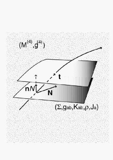
Figure 1: An admissible set of initial data is propagated along the time–like vector field $\mathbf{t}=\mathbf{n}N+\mathbf{N}$, with the lapse function $N$ scaling the unit normal $\mathbf{n}$ at the given point and the shift vector field $\mathbf{N}$. The spacetime geometry is foliated into hypersurfaces $\Sigma$, $(M^{(4)}\simeq\Sigma\times\mathbb{R},g^{(4)})$, on which we study scaling properties of the initial data set.

Thus, it seems appropriate to recall some of the properties of the Arnowitt–Deser–Misner formulation of Einstein’s equations. This essentially exploits the fact that a globally hyperbolic spacetime $(M^{(4)},g^{(4)})$ is diffeomorphic to $\mathbb{R}\times\Sigma$, where $\Sigma$ is a three–dimensional manifold which we assume (for simplicity) to be closed. The explicit diffeomorphism $\varphi:\mathbb{R}\times\Sigma\rightarrow M^{(4)}$ is constructed by defining on $M^{(4)}$ a timelike vector field $\mathbf{t}$ the integral curves of which, $\Phi(t,p)$, define a map $f:\Sigma\rightarrow M^{(4)}$ according to $p\longmapsto f(p)=\Phi(t,p)$, (for each given $t\in\mathbb{R}$). Consider, in such a setting, the dynamics of a self–gravitating distribution of matter. In the ADM formulation, the dynamics of such a distribution and the corresponding spacetime geometry $(M^{(4)}\simeq\Sigma\times\mathbb{R},g^{(4)})$ are described by the evolution of an initial data set:

$$(\;\;\Sigma\;,\;g_{ab}\;,\;K_{ab}\;,\;\varrho\;,\;J_{a}\;\;)$$ (1)

where the Riemannian metric $g_{ab}$ and the triple of tensor fields $(K_{ab},\varrho,J_{a})$, are subjected to the Hamiltonian and divergence constraints:

$${\cal R}+{K}^{2}-K^{a}_{\;\,b}K^{b}_{\;\,a} = 16\pi G\varrho+2\Lambda\;,$$ (2)

$$\nabla_{b}K^{b}_{\;\,a}-\nabla_{a}K = 8\pi GJ_{a}\;,$$ (3)

where $K:=g^{ab}K_{ab}$ is the trace of the extrinsic curvature $K_{ab}$, ${\cal R}:=g^{ab}{\cal R}_{ab}$ is the trace of the intrinsic Ricci curvature of the metric $g_{ab}$, and $\Lambda$ is the cosmological constant. If such a set of admissible data is propagated according to the evolutive part of Einstein’s equations, then the symmetric tensor field $K_{ab}$ can be interpreted as the second fundamental form of the embedding of $(\Sigma,g_{ab})$ in the spacetime $(M^{(4)}\simeq\Sigma\times\mathbb{R},g^{(4)})$ resulting from the evolution of $(\Sigma,g_{ab},K_{ab},\varrho,J_{a})$, whereas $\varrho$ and $J_{a}$ are, respectively, identified with the mass density and the momentum density of the material self–gravitating sources on $(\Sigma,g_{ab})$. Explicitly, the evolution equations associated with the initial data $(\Sigma,g_{ab},K_{ab},\varrho,J_{a})$ are provided (in the absence of stresses, i.e., for a dust matter model) by

$$\frac{\partial g_{ab}}{\partial t}=-2NK_{ab}+{\cal L}_{\vec{N}}g_{ab}\;,$$ (4)

$$\frac{\partial K_{ab}}{\partial t}=-\nabla_{a}\nabla_{b}N+N\left[KK_{ab}+{\cal R}_{ab}-(4\pi G\varrho+\Lambda)g_{ab}\right]+{\cal L}_{\vec{N}}K_{ab}\;,$$ (5)

where $N$ and $\vec{N}$, respectively, denote the lapse function and the shift vector field associated with the mapping $f:\Sigma\rightarrow M^{(4)}$ (i.e., $\vec{t}=N\vec{n}+\vec{N}$, $\vec{n}$ being the future–pointing unit normal to the embedding $\Sigma\hookrightarrow M^{(4)}$ (Fig. 1)).

For the discussion of scaling properties and the averaging procedure associated with an admissible set of initial data $(\Sigma,g_{ab},K_{ab},\varrho,J_{a})$ for a cosmological spacetime $(M^{(4)}\simeq\Sigma\times\mathbb{R},g^{(4)})$ we start by characterizing explicitly a scale–dependent averaging for the empirical mass distribution $\varrho$.

1.1 Interlude: matter seen at different scales

In order to characterize the scale over which we are smoothing the empirical mass distribution $\varrho$, we need to study the distribution $\varrho$ by looking at its average behavior on regional domains (geodesic balls) in $(\Sigma,g_{ab})$ with different centers and radii. The idea is to move from the function $\varrho:\Sigma\rightarrow\mathbb{R}^{+}$ to an associated function, defined on $\Sigma\times\mathbb{R}^{+}$, and which captures some aspect of the behavior of the given $\varrho$ on average, at different scales and locations. The simplest function of this type is provided by the regional volume average:

$$\left\langle\varrho\right\rangle_{B(p;r)}:=\frac{1}{V\left(B(p;r)\right)}\int_{B(p;r)}\varrho\;d\mu_{g},$$ (6)

where $p\in\Sigma$ is a generic point, $d\mu_{g}$ is the Riemannian volume element associated with $(\Sigma,g_{ab})$, and $B(p;r)$ denotes the geodesic ball at center $p$ and radius $r$ in $(\Sigma,g_{ab})$ (Fig. 2), i.e.,

$$B(p;r):=\left\{q\in(\Sigma,g_{ab})\,:d_{g}(p,q)\leq r\,\,\right\},$$ (7)

where $d_{g}(p,q)$ denotes the distance, in $(\Sigma,g_{ab})$, between the point $p$ and $q$. Note that if

$$diam:=\sup\left\{d_{g}(p,q)\,:p,q\in(\Sigma,g_{ab})\right\}$$ (8)

denotes the diameter of $(\Sigma,g_{ab})$, then as $r\rightarrow diam$, we get

$$\left\langle\varrho\right\rangle_{B(p;r)}\longrightarrow\left\langle\varrho\right\rangle_{\Sigma}:=\frac{1}{V(\Sigma)}\int_{\Sigma}\varrho\;d\mu_{g},$$ (9)

at any point

$p\in\Sigma$. Conversely, if $\varrho:\Sigma\rightarrow\mathbb{R}^{+}$ is locally summable, then

$$\lim_{r\rightarrow 0}\,\left\langle\varrho\right\rangle_{B(p;r)}=\varrho(p)\;,$$ (10)

for almost all points $p\in\Sigma$. The passage from $\varrho$ to $\left\langle\varrho\right\rangle_{B(p;r)}$ corresponds to replacing the position–dependent empirical distribution of matter in $B(p;r)$ by a regionally uniform distribution $\left\langle\varrho\right\rangle_{B(p;r)}$ which is constant over the typical scale $r$. Note that for the total (material) mass contained in $B(p;r)$, we get

$$M(B(p;r)):=\int_{B(p;r)}\varrho\;d\mu_{g}=V\left(B(p;r)\right)\left\langle\varrho\right\rangle_{B(p;r)},$$ (11)

and

$$\lim_{r\rightarrow diam}M(B(p;r))=M(\Sigma):=\int_{\Sigma}\varrho\;d\mu_{g},$$ (12)

where $M(\Sigma)$ is the total (material) mass contained in $(\Sigma,g_{ab})$. Our expectations in $\left\langle\varrho\right\rangle_{B(p;r)}$ are motivated by the fact that on Euclidean $3$–space $(\mathbb{R}^{3},\delta_{ab})$, if $\varrho$ is a bounded function, then the regional average $\left\langle\varrho\right\rangle_{B(p;r)}$ is a Lipschitz function on $\mathbb{R}^{3}\times\mathbb{R}^{+}$, endowed with the hyperbolic metric [41]:

$$\frac{dx_{1}^{2}+dx_{2}^{2}+dx_{3}^{2}+dr^{2}}{r^{2}}.$$ (13)

In other words,

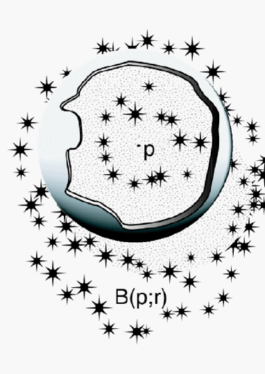
Figure 2: The domain of averaging, centred on a given point $p$, is a (possibly non–convex) simply–connected geodesic ball domain contained in the hypersurface. The diagnostic parameter to explore the manifold is the radius $r$ of the geodesic ball. It is mapped from the “master ball” with Euclidean geometry into the manifold by the exponential mapping. The shape of the ball’s surface reflects the inhomogeneous geometry of the hypersurface at the scale $r$; the ball encloses a portion of the inhomogeneous matter distribution (marked by stars) interacting with the environmental distribution.

$$\left|\left\langle\varrho\right\rangle_{B(p;r)}-\left\langle\varrho\right\rangle_{B(q;r)}\right|\leq C_{0}d_{h}(p,q),$$ (14)

where $C_{0}$ is a constant and $d_{h}(p,q)$ is the (hyperbolic) distance between $p$ and $q$. Thus, the regional averages $\left\langle\varrho\right\rangle_{B(p;r)}$ do not oscillate too wildly as $p$ and $r$ vary, and the replacement of $\varrho$ by $\{\left\langle\varrho\right\rangle_{B(p;r)}\}_{p\in\mathbb{R}^{3}}$ indeed provides an averaging of the original matter distribution over the length scale $r$. It is not obvious that such a nice behavior carries over to the Riemannian manifold $(\Sigma,g_{ab})$. The point is that, even if the regional averages $\{\left\langle\varrho\right\rangle_{B(p;r)}\}_{p\in\Sigma}$ provide a controllable device of smoothing the matter distribution at the given scale $r$ (see: Remark 1), they still depend in a sensible way on the geometry of the typical ball $B(p;r)$ as we vary the averaging radius. In this connection we need to understand how, as we rescale the domain $B(p;r)$, the regional average $\left\langle\varrho\right\rangle_{B(p;r)}$ depends on the underlying geometry of $(\Sigma,g_{ab})$. The reasoning here is slightly delicate, so we go into a few details that require some geometric preliminaries.

Geometrical evolution of geodesic ball domains

Let us denote by

$$\exp_{p}:T_{p}\Sigma\rightarrow\Sigma$$

$$(\vec{v},r)\longmapsto\exp_{p}(r\vec{v})$$ (15)

the exponential mapping at $p\in(\Sigma,g_{ab})$, i.e., the map which to the vector $r\vec{v}\in T_{p}\Sigma\simeq\mathbb{R}^{3}$ associates the point $\exp_{p}(r\vec{v})\in\Sigma$ reached at “time” $r\in\mathbb{R}_{+}$ by the unique geodesic issued at $p\in\Sigma$ with unit speed $\vec{v}\in\mathbb{S}^{2}(1)$ . Let $r>0$ be such that $\exp_{p}$ is defined on the Euclidean ball

$$B_{E}(0,r):=\{y\in T_{p}\Sigma\simeq\mathbb{R}^{3}:|y|\leq r\}$$ (16)

and $\exp_{p}:B_{E}(0,r)\rightarrow B(p,r)\subset\Sigma$ is a diffeomorphism onto its image. The largest radius $r$ for which this is true, as $p$ varies in $\Sigma$, is called the injectivity radius $\mathrm{inj}_{M}$ of $(\Sigma,g_{ab})$ (Fig. 3).

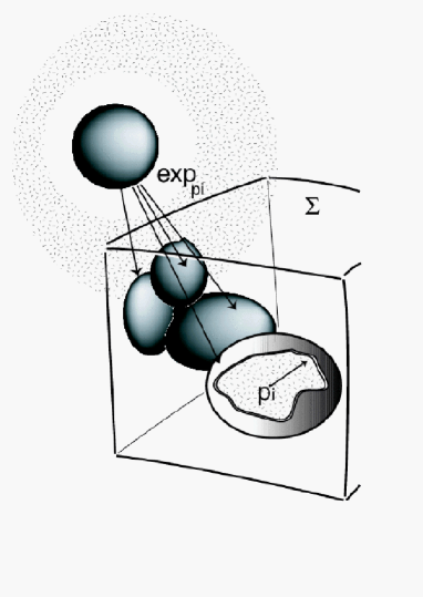
Figure 3: Four ball domains mapped by the exponential mapping from the Lagrangian “master ball” into the Riemannian manifold are shown. Notice that the ball domains may overlap. The possible case in which they lie in topologically disconnected pieces of the manifold is excluded due to our choice of a maximal radius.

Let $B(p;r_{0})$ denote a given geodesic ball of radius $r_{0}<\mathrm{inj}_{M}$, and for vector fields $X$, $Y$, and $Z$, in $(B(p;r),g_{ab})$ let $\mathcal{R}(X,Y)Z=\mathcal{R}_{\;\,bcd}^{a}X^{c}Y^{d}Z^{b}$ $\partial_{a}$ be the corresponding curvature tensor. Since $r:(B(p;r),g_{ab})\rightarrow\mathbb{R}$ is a distance function (i.e., $|\nabla r|\equiv 1$), the geometry of $B(p;r)$ can be described by the following set of equations [38]:

$$(\nabla_{\partial_{r}}S)(X)+S^{2}(X)=-{\cal R}(X,\partial_{r})\partial_{r},$$ (17)

$$({\cal L}_{\partial_{r}}g)(X,Y)=2g(S(X),Y),$$ (18)

$$\nabla_{\partial_{r}}S={\cal L}_{\partial_{r}}S,$$ (19)

where $\partial_{r}=\nabla r$ is the gradient of $r$, ${\cal L}_{\partial_{r}}g$ is the Lie derivative of the 3–metric $g$ in the radial direction $\partial_{r}$, the shape tensor $S=\nabla^{2}r$ is the Hessian of $r$, and $S^{2}(X)$ abbreviates $S^{2}(X)=S^{\alpha}_{\;\,\eta}S^{\eta}_{\;\,\beta}X^{\beta}\partial_{\alpha}$. Such equations follow from the Gauss–Weingarten relations applied to study the $r$–constant slices $U_{r}:=\{\exp_{p}(r\vec{v})\in\Sigma:r=const.\}$, which are the images in $(B(p;r),g_{ab})$ of the standard Euclidean $2$–spheres $\mathbb{S}^{2}(r)\subset T_{p}\Sigma\simeq\mathbb{R}^{3}$. The shape tensor $S_{ab}$ measures how the bidimensional metric $g^{(2)}(X,Y)$ induced on $U_{r}$ by the embedding in $(B(p;r),g_{ab})$ rescales as the radial distance $r$ varies. If we denote by $P_{U}(W):=W-g(W,\partial_{r})\partial_{r}$ the tangential projection of a vector $W\in T_{p}\Sigma$ onto the tangent space $T_{p}U$ to the surface $U_{r}$ at $p$, then together with (17), (18), (19) we also get the tangential curvature equation:

$$P_{U}\left({\cal R}(X,Y)Z\right)=$$

$${\cal G}\left(g^{(2)}(Y,Z)X-g^{(2)}(X,Z)Y\right)-g^{(2)}(S(Y),Z)S(X)-g^{(2)}(S(X),Z)S(Y)\;,$$ (20)

where the vectors $X$ and $Y$ are tangent to $U_{r}$, and where $\cal G$ denotes the Gaussian curvature of $(U_{r},g^{(2)})$. Further properties of the equations (17) and (18) that we need are best seen by using polar geodesic coordinates. Recall that normal exponential coordinates at $p$ are geometrically defined by

$$\exp_{p}^{-1}:B(p;r)\rightarrow T_{p}\Sigma\simeq\mathbb{R}^{3}\;\;\;;\;\;\;q\longmapsto\exp_{p}^{-1}(q)=(y^{i})\;\;,$$ (21)

where $(y^{i})$ are the Cartesian components of the velocity vector $\vec{v}\in$ $T_{p}\Sigma$ characterizing the geodesic segment from $p$ to $q$. Such coordinates are unique up to the chosen identification of $T_{p}\Sigma$ with $\mathbb{R}^{3}$. Since we are dealing with a radial rescaling, for our purposes a suitable identification is the one associated with the use of polar coordinates in $T_{p}\Sigma\simeq\mathbb{R}^{3}$. We therefore introduce an orthonormal frame $\{e_{1},e_{2},e_{3}\}$ in $T_{p}\Sigma$ such that $e_{1}:=\partial_{r}$ and with $\{e_{2},e_{3}\}$ an orthonormal frame on the unit $2$–sphere $\mathbb{S}^{2}(1)\subset T_{p}\Sigma$. We can extend such vector fields radially to the whole $T_{p}\Sigma$; we consider also the dual coframe ${\theta^{2},\theta^{3}}$ associated with ${e_{2},e_{3}}$. The introduction of such a polar coordinate system in $T_{p}\Sigma$ is independent of the metric $g_{ab}$ and thus is ideally suited for discussing geometrically the $r$–scaling properties of $\left\langle\varrho\right\rangle_{B(p;r)}$ (see, however, Remark 2). If we pull–back to $T_{p}\Sigma$ the metric $g$ of $B(p;r)\subset\Sigma$, we get:

$$g=dr^{2}+g(e_{\alpha},e_{\beta})\theta^{\alpha}\theta^{\beta},\;\alpha,\beta=2,3,$$ (22)

where the components $g_{\alpha\beta}:=g(e_{\alpha},e_{\beta})$ $=g^{(2)}(r,\vartheta,\varphi)$ are functions of the polar coordinates $(\vartheta,\varphi)$ in $T_{p}\Sigma\simeq\mathbb{R}^{3}$, associated with the coframe ${\theta^{2},\theta^{3}}$. Note that such a local representation of the metric holds throughout the local chart $(B(p;r),\exp_{p}^{-1})$ and not just at $p$. In Cartesian coordinates in $T_{p}\Sigma\simeq\mathbb{R}^{3}$ one recovers the familiar expression:

$$g_{ab}=\delta_{ab}-\frac{1}{3}\mathcal{R}_{akbl}(p)y^{k}y^{l}+\mathcal{O}\left(|y|^{3}\right)\;.$$ (23)

In polar geodesic coordinates we have $(x^{1}:=r,x^{2}:=\vartheta,x^{3}:=\varphi)$ and $g_{\alpha\beta}^{(2)}=g_{\alpha\beta}$ with $2\leq\alpha,\beta\leq 3$. Thus the equations (17), and (18) take the explicit form:

$$\partial_{r}S_{\;\,\beta}^{\alpha}=-S_{\;\,\eta}^{\alpha}S_{\;\,\beta}^{\eta}-{\cal R}_{\;\,r\beta r}^{\alpha}\;\;;$$ (24)

$$\partial_{r}g_{\alpha\beta}=2S_{\;\,\alpha}^{\eta}g_{\eta\beta}\;\;,$$ (25)

where ${\cal R}_{\;\,r\beta r}^{\alpha}$ denote the radial components of the curvature tensor. According to the tangential Gauss–Codazzi equation (20) we can also write

$$R_{\;\,\mu\beta\nu}^{\alpha}={\cal G}\left(\delta_{\;\,\beta}^{\alpha}g_{\nu\mu}-\delta_{\;\,\nu}^{\alpha}g_{\beta\mu}\right)-S_{\;\,\beta}^{\alpha}S_{\nu\mu}+S_{\;\,\nu}^{\alpha}S_{\beta\mu}\;.$$ (26)

If we introduce the tangential components of the Ricci tensor according to

$${\cal R}_{\;\,\beta}^{\alpha}:=g^{kl}{\cal R}_{\;\,k\beta l}^{\alpha}={\cal R}_{\;\,r\beta r}^{\alpha}+{\cal G}\delta_{\;\,\beta}^{\alpha}-S_{\;\,\beta}^{\alpha}S+S_{\;\,\nu}^{\alpha}S_{\;\,\beta}^{\nu}\;,$$ (27)

then we can rewrite the radial components of the curvature as

$${\cal R}_{\;\,r\beta r}^{\alpha}={\cal R}_{\;\,\beta}^{\alpha}-{\cal G}\delta_{\;\,\beta}^{\alpha}+S_{\;\,\beta}^{\alpha}S-S_{\;\,\nu}^{\alpha}S_{\;\,\beta}^{\nu}\;,$$ (28)

and the first of equations (25) becomes

$$\partial_{r}S_{\;\,\beta}^{\alpha}=-{\cal R}_{\;\,\beta}^{\alpha}+{\cal G}\delta_{\;\,\beta}^{\alpha}-S_{\;\,\beta}^{\alpha}S\;,$$ (29)

where $S:=S_{\;\,\beta}^{\alpha}\delta_{\;\,\beta}^{\alpha}$ is the rate of area expansion of $g^{(2)}(r,\vartheta,\varphi)$. Note that by taking the trace of both equations (25) we get:

$$\partial_{r}S=-S_{\;\,\nu}^{\alpha}S_{\;\,\alpha}^{\nu}-Ric(\partial_{r},\partial_{r})\;,$$ (30)

$$g^{\alpha\beta}\partial_{r}g_{\alpha\beta}=2S\;,$$ (31)

where $Ric(\partial_{r},\partial_{r}):=$ ${\cal R}_{\;\,rir}^{i}$ denotes the $\partial_{r}$ component of the Ricci tensor, (the first equation in (30) is nothing but the Jacobi operator coming from the second variation of the area associated with $g^{(2)}(r,\vartheta,\varphi)$). If we assume that the curvature ${\cal R}(X,Y)Z$ is given, then, by fixing the $(\vartheta,\varphi)$–dependence in the factorized metric (22), we can consider (25) as a system of decoupled ordinary differential equations describing the rescaling of the geometry of $B(p;r)$ in terms of the one–parameter flow of immersions $\mathbb{S}^{2}(r)\mapsto$ $(U_{r},g^{(2)}(r,\vartheta,\varphi))$. Note in particular that the shape tensor matrix $(S_{\;\,\beta}^{\alpha})$ is characterized, from the equation (29), as a functional of the Ricci curvature of the ambient manifold $(\Sigma,g_{ab})$.

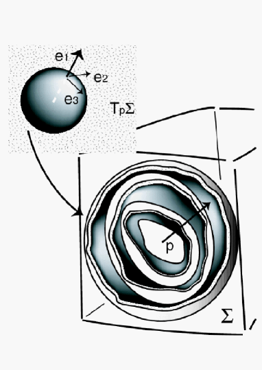
Figure 4: A foliation of the geodesic ball along the radial direction into a family of geodesic balls is shown. The metric on the boundary of the balls factorizes into radial and tangential components due to our choice of the Dreibein $e_{1},e_{2},e_{3}$ in the “master ball”.

Scaling properties of the metric

In such a setting the equation $\partial_{r}g_{\alpha\beta}=2S_{\;\,\alpha}^{\eta}g_{\eta\beta}$ can be interpreted by saying that the metric rescales radially along the (curvature–dependent) shape tensor $S_{\;\,\beta}^{\alpha}$. In order to get a more explicit expression of such a radial rescaling, let us consider, at a fixed $r_{0}$, a one–parameter family of surfaces $(U_{r},g^{(2)}(r,\vartheta,\varphi))$ with parameter $(r-r_{0})\geq 0$ starting at the given surface $(U_{r_{0}},g^{(2)}(r_{0},\vartheta,\varphi))$ and foliating the ball $B(p;r)$ (Fig. 4). In a sufficiently small neighborhood of the initial surface $(U_{r_{0}},g^{(2)}(r_{0},\vartheta,\varphi))$, we can write

$$S_{\;\,\beta}^{\alpha}(r)=S_{\;\,\beta}^{\alpha}(r_{0})+\left[-{\cal R}_{\;\,\beta}^{\alpha}+{\cal G}\delta^{\alpha}_{\;\,\beta}-S^{\alpha}_{\;\,\beta}S\right]_{r_{0}}(r-r_{0})+\mathcal{O}((r-r_{0})^{2})\;.$$ (32)

Inserting such an expression into $\partial_{r}g_{\alpha\beta}=2S_{\;\,\alpha}^{\eta}g_{\eta\beta}$ we get

$$\frac{1}{(r-r_{0})}\left[\partial_{r}g_{\alpha\beta}(r)-\partial_{r}g_{\alpha\beta}(r)|_{r_{0}}\right]=$$

$$-2{\cal R}_{\alpha\beta}(r_{0})+2\left[{\cal G}\delta_{\alpha\beta}-S_{\alpha\beta}S\right]_{r_{0}}+\mathcal{O}((r-r_{0}))\;.$$ (33)

Note that the terms $2\left[{\cal G}\delta_{\alpha\beta}-S_{\alpha\beta}S\right]_{r_{0}}$ only depend on the geometry (intrinsic and extrinsic) of the surface $(U_{r_{0}},g^{(2)}(r_{0},\vartheta,\varphi))$ and represent reaction tangential terms which work against the curvature of the ambient $(\Sigma,g_{ab})$. Thus, one may say that in a sufficiently small neighborhood of the initial surface $(U_{r_{0}},g^{(2)}(r_{0},\vartheta,\varphi))$ the ambient geometry of $(\Sigma,g_{ab})$ forces the metric to rescale radially in the direction of its Ricci tensor. This latter remark will turn out quite useful in understanding the geometric rationale behind the choice of a proper averaging procedure for the geometry of $(\Sigma,g_{ab})$.

Scaling properties of the averaged density field

Guided by such geometrical features of geodesic balls, let us go back to the study of the scaling properties of $\left\langle\varrho\right\rangle_{B(p;r)}$. To this end, for any $r$ and $s$ such that $r+s<{\rm inj}_{\Sigma}$, let us consider the one–parameter family of diffeomorphisms

$$H_{s}:(\Sigma,p)\rightarrow(\Sigma,p)$$

$$q=\exp_{p}[r_{q}(\partial_{r},e_{2},e_{3})]\longmapsto H_{q}(q):=\exp_{p}[(r_{q}+s)(\partial_{r},e_{2},e_{3})]\;,$$ (34)

defined by flowing each point $q\in B(p;r)$ a distance $s$ along the unique radial geodesic segment issued at $p\in\Sigma$ and passing through $q$. Let us remark that, for any $r$ such that $r_{0}\leq r<{\rm inj}_{M}$, we can formally write

$$B(p;r)=H_{(r-r_{0})}B(p;r_{0}).$$ (35)

Thus, in a neighborhood of $B(p;r_{0})$ and for sufficiently small $r$, we get

$$M(B(p;r)):=\int_{B(p;r)}\varrho\;d\mu_{g}=\int_{B(p;r_{0})}H_{(r-r_{0})}^{\ast}(\varrho\;d\mu_{g}),$$ (36)

where $H_{(r-r_{0})}^{\ast}(\varrho d\mu_{g})$ is the Riemannian measure obtained by pulling back ($\varrho\,d\mu_{g}$) under the action of $H_{(r-r_{0})}$. By differentiating (36) with respect to $r$, we have:

$$\frac{d}{dr}M(B(p;r))=\lim_{h\rightarrow 0}\frac{\left[M(B(p;r+h))-M(B(p;r))\right]}{h}$$

$$=\lim_{h\rightarrow 0}\frac{\left[\int_{B(p;r_{0})}H_{(r-r_{0})+h}^{\ast}(\varrho\;d\mu_{g})-\int_{B(p;r_{0})}H_{(r-r_{0})}^{\ast}(\varrho\;d\mu_{g})\right]}{h}\;\;.$$ (37)

Since $H_{(r-r_{0})+h}=H_{(r-r_{0})}\circ H_{h}$, we can write the above expression as:

$$\lim_{h\rightarrow 0}\left[\int_{B(p;r_{0})}\frac{H_{(r-r_{0})}^{\ast}\left[H_{h}^{\ast}(\varrho\;d\mu_{g})-(\varrho\;d\mu_{g})\right]}{h}\right]$$

$$=\lim_{h\rightarrow 0}\left[\int_{B(p;r)}\frac{\left[H_{h}^{\ast}(\varrho\;d\mu_{g})-(\varrho\;d\mu_{g})\right]}{h}\right]\;=\;\int_{B(p;r)}\lim_{h\rightarrow 0}\frac{\left[H_{h}^{\ast}(\varrho\;d\mu_{g})-(\varrho\;d\mu_{g})\right]}{h}\;,$$ (38)

from which it follows that (use ${\cal L}_{\partial_{r}}d\mu_{g}={\rm div}(\partial_{r})d\mu_{g}$ and ${\cal L}_{\partial_{r}}\varrho=d\varrho(\partial_{r})=\frac{\partial}{\partial r}\varrho$):

$$\frac{d}{dr}M(B(p;r))=\int_{B(p;r)}{\cal L}_{\partial_{r}}\varrho\;d\mu_{g}$$

$$=\int_{B(p;r)}\left({\cal L}_{\partial_{r}}\varrho+\varrho{\rm div}(\partial_{r})\right)\;d\mu_{g}\;=\;\int_{B(p;r)}\left(\frac{\partial}{\partial r}\varrho+\frac{1}{2}\varrho g^{ab}\frac{\partial}{\partial r}g_{ab}\right)\;d\mu_{g}\;\;,$$ (39)

where ${\cal L}_{\partial_{r}}$ and ${\rm div}(\partial_{r})$ denote the Lie derivative along the vector field $\partial_{r}$ and its divergence, respectively, and where we have exploited the well–known expression for the Lie derivative of a volume density along $\partial_{r}$:

$$\frac{\partial}{\partial r}\sqrt{g}=\frac{1}{2}\sqrt{g}g^{ab}\frac{\partial}{\partial r}g_{ab}\;\;.$$ (40)

With these preliminary remarks along the way, it is straightforward to compute the total rate of variation with $r$ of the regional average $\left\langle\varrho\right\rangle_{B(p;r)}$, since (1.1) implies:

$$\frac{\partial}{\partial r}\left\langle\varrho\right\rangle_{B(p;r)}=\left\langle\frac{\partial}{\partial r}\varrho\right\rangle_{B(p;r)}$$

$$+\;\frac{1}{2}\left\langle\varrho g^{ab}\frac{\partial}{\partial r}g_{ab}\right\rangle_{B(p;r)}\;-\;\frac{1}{2}\left\langle\varrho\right\rangle_{B(p;r)}\left\langle g^{ab}\frac{\partial}{\partial r}g_{ab}\right\rangle_{B(p;r)}\;,$$ (41)

where $\left\langle f\right\rangle_{B(p;r)}$ denotes the volume average of $f$ over the ball $B(p;r)$. Explicitly, by exploiting (25), we get

$$\frac{\partial}{\partial r}\left\langle\varrho\right\rangle_{B(p;r)}=\left\langle\frac{\partial}{\partial r}\varrho\right\rangle_{B(p;r)}+\left\langle\varrho S\right\rangle_{B(p;r)}-\left\langle\varrho\right\rangle_{B(p;r)}\left\langle S\right\rangle_{B(p;r)}.$$ (42)

Thus, the regional average $\left\langle\varrho\right\rangle_{B(p;r)}$ feels the fluctuations in the geometry as we vary the scale, fluctuations represented by the shape tensor terms

$$\left\langle\varrho S\right\rangle_{B(p;r)}-\left\langle\varrho\right\rangle_{B(p;r)}\left\langle S\right\rangle_{B(p;r)}$$ (43)

governed by the curvature in $B(p;r)$ according to (30), and expressing a geometric non–commutativity between averaging over the ball $B(p;r)$ and rescaling its size (Fig. 5). Since the curvature varies both in the given $B(p;r)$ and when we consider distinct base points $p$, the above remarks indicate that the regional averages $\left\langle\varrho\right\rangle_{B(p;r)}$ are subjected to the accidents of the fluctuating geometry of $(\Sigma,g_{ab})$. In other words, there is no way of obtaining a proper smoothing of $\varrho$ without smoothing out at the same time the geometry of $(\Sigma,g_{ab})$.

Non–commutativity of averaging and scaling

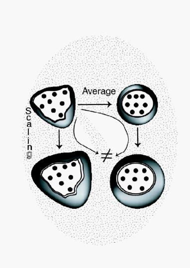
Figure 5: Volume–averaging scalar fields over the geodesic ball, and rescaling the radius of the ball are non–commuting operations. Note that a Lagrangian averaging as well as a rescaling to first order in the radius preserves the material mass content of the ball.

It is straightforward to generalize the foregoing result for any smooth scalar function $\psi$ yielding a rule that summarizes the key result of this subsection.

Proposition 1   (Commutation Rule)

On a Riemannian hypersurface $(\Sigma,g_{ab})$ volume–averaging on a geodesic ball $B(p;r)$ and scaling (directional derivative along the vector field $\frac{\partial}{\partial r}$) of a scalar function $\psi$ are non–commuting operations, as can be expressed by the rule:

$$\frac{\partial}{\partial r}\langle\psi\rangle_{B(p;r)}-\langle\frac{\partial}{\partial r}\psi\rangle_{B(p;r)}=\langle S\psi\rangle_{B(p;r)}-\langle S\rangle_{B(p;r)}\langle\psi\rangle_{B(p;r)}\;;$$

$$S=\frac{1}{\sqrt{g}}\frac{\partial}{\partial r}\sqrt{g}\;\;;\;\;\langle S\rangle_{B(p;r)}=\frac{1}{V(B(p;r))}\frac{\partial}{\partial r}V(B(p;r))\;.$$ (44)

Note that this formula may also be read as follows:

$$\frac{\partial}{\partial r}\langle\psi\rangle_{B(p;r)}+\langle S\rangle_{B(p;r)}\langle\psi\rangle_{B(p;r)}=\langle\frac{\partial}{\partial r}\psi+S\psi\rangle_{B(p;r)}\;.$$ (45)

1.2 Eulerian averaging and Lagrangian smoothing

The use of the exponential mapping in discussing the geometry behind the regional averages $\left\langle\varrho\right\rangle_{B(p;r)}$ makes it clear that we are trying to measure how different the averages $\left\langle\varrho\right\rangle_{B(p;r)}$ are from the standard average over Euclidean balls. In so doing we think of  $\exp_{p}:T_{p}\Sigma\rightarrow\Sigma$ as maps from the fixed space $B_{E}(0,r)$ into the manifold $(\Sigma,g_{ab})$. In this way we are implicitly trying to transfer information from the manifold $(\Sigma,g_{ab})$ into domains of $\mathbb{R}^{3}$ which we would like to be, as far as possible, independent of the accidental geometry of $(\Sigma,g_{ab})$ itself. Indeed, any averaging would be quite difficult to implement, if the reference model varies with the geometry to be averaged. This latter task is only partially accomplished by the exponential mapping, since the domain over which $\exp_{p}:T_{p}\Sigma\rightarrow\Sigma$ is a diffeomorphism depends on $p$ and on the actual geometry of $(\Sigma,g_{ab})$. A suitable alternative is to use harmonic coordinates in the ball $B(p;r)$, a technique which is briefly discussed in Remark 2.

We now go a step further by considering not just the given $(\Sigma,g_{ab})$, but rather a whole family of Riemannian manifolds. To start with let us remark that, if we fix the radius $r_{0}$ of the Euclidean ball $B_{E}(0;r_{0})\subset T_{p}\Sigma$ and consider the family of exponential mappings, $\exp_{(p,\beta)}:T_{p}\Sigma\rightarrow(\Sigma,g_{ab}(\beta))$, associated with a corresponding one–parameter family of Riemannian metrics $g_{ab}(\beta)$, $0\leq\beta<+\infty$, with $g_{ab}(\beta=0)=g_{ab}$, then $B(p;r_{0})$ becomes a functional of the set of Riemannian structures associated with $g_{ab}(\beta)$, $0\leq\beta<+\infty$, i.e.,

$$B(p;r_{0})\longmapsto B_{\beta}(p;r_{0}):=\exp_{(p,\beta)}\left[B_{E}(0;r_{0})\right].$$ (46)

In this way, instead of considering just a given geodesic ball $B(p;r_{0})$, we can consider, as $\beta$ varies, a family of geodesic balls $B_{\beta}(p;r_{0})$, all with the same radius $r_{0}$ but with distinct inner geometries $g_{ab}(\beta)$. Since $B_{\beta=0}(p;r_{0})=B(p;r_{0})$, such balls can be thought of as being obtained from the given one $B(p;r_{0})$ by a smooth continuous deformation of its original geometry. Under such deformation also $\left\langle\varrho\right\rangle_{B(p;r_{0})}$ becomes $\beta-$dependent due to the functional dependence $\left\langle\varrho\right\rangle_{B_{\beta}(p;r_{0})}$.

The elementary but basic observation in order to take proper care of the geometrical fluctuations in $\left\langle\varrho\right\rangle_{B(p;r_{0})}$ is that the right member of (41) has precisely the formal structure of the linearization ( i.e., of the variation) of the functional $\left\langle\varrho\right\rangle_{B(p;r_{0})}$ in the direction of the deformed Riemannian metric $\frac{\partial}{\partial\beta}[g_{ab}(\beta)]$, viz.,

$$\frac{\partial}{\partial\beta}\left\langle\varrho\right\rangle_{B_{\beta}(p;r_{0})}=\left\langle\frac{\partial}{\partial\beta}\varrho\right\rangle_{B_{\beta}(p;r_{0})}$$

$$+\;\frac{1}{2}\left\langle\varrho g^{ab}(\beta)\frac{\partial}{\partial\beta}g_{ab}(\beta)\right\rangle_{B_{\beta}(p;r_{0})}\;-\;\frac{1}{2}\left\langle\varrho\right\rangle_{B_{\beta}(p;r_{0})}\left\langle g^{ab}(\beta)\frac{\partial}{\partial\beta}g_{ab}(\beta)\right\rangle_{B_{\beta}(p;r_{0})}\;,$$ (47)

where the ball $B_{E}(0;r_{0})$ is kept fixed while its image $B(p;r_{0})$ is deformed according to the flow of metrics $g_{ab}(\beta)$, $0\leq\beta\leq\infty$ (Fig. 6).

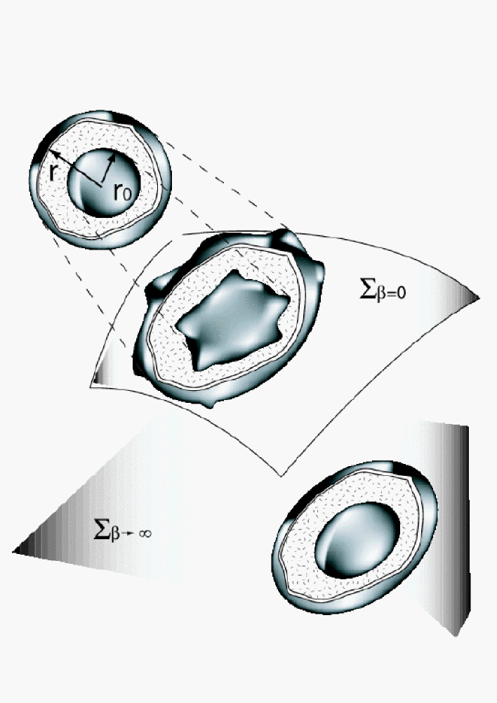
Figure 6: Averaging over geodesic ball domains, while scaling the geodesic radius is conceptually (and formally) equivalent with their Lagrangian deformation for fixed geodesic radius. The transformation of a Lagrangian ball is illustrated with respect to $r-$scaling and $\beta-$deformation.

In a rather obvious sense, (47) represents the active interpretation corresponding to the Eulerian passive view associated with the ball variation $B(p;r_{0})\rightarrow B(p;r)$. In other words, we are here dealing with the (geometrical) Lagrangian point of view of following a fluid domain in its deformation, where the fluid particles here are the points of $B(p;r_{0})$ suitably labelled. This latter remark suggests that in order to optimize the averaging procedure associated with the regional average $\left\langle\varrho\right\rangle_{B(p;r)}$, instead of studying its scaling behavior as $r$ increases, and consequently be subjected to the accidents of the fluctuating geometry of $(B(p;r),g_{ab})$, we may keep fixed the domain $B_{E}(0;r_{0})$ (setting the scale over which we are averaging) and rescale the geometry inside its image $B(p;r_{0})$ under the exponential map, according to a suitable flow of metrics $g_{ab}\rightarrow g_{ab}(\beta)$, $0\leq\beta\leq\infty$. Correspondingly, also the average matter density will be forced to rescale $\langle\varrho\rangle_{B(p;r_{0})}\rightarrow\langle\varrho\rangle_{B_{\beta}(p;r_{0})}(\beta)$, and if we are able to choose the flow $g_{ab}\rightarrow g_{ab}(\beta)$ in such a way that the local inhomogeneities of the original geometry of $(\Sigma,g_{ab})$ are smoothly eliminated, then the regional averages $\left\langle\varrho\right\rangle_{B_{\beta}(p;r_{0})}$ come closer and closer to represent a matter averaging over a homogeneous geometry.

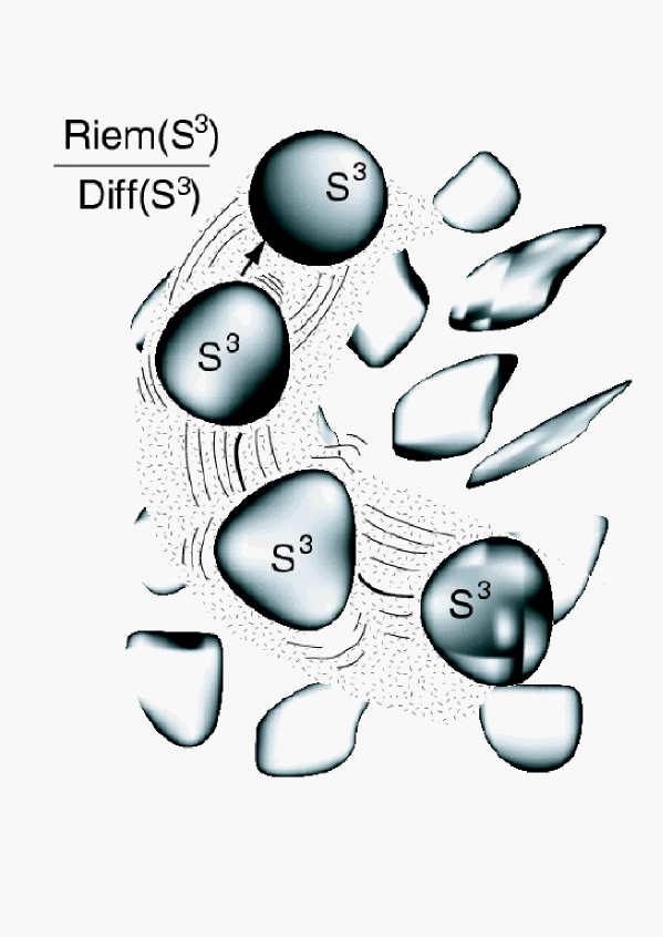
Figure 7: When it is global, the Ricci flow acts in the space of all possible Riemannian geometries by smoothing the geometry in a controllable fashion: here we depict the case of a three–sphere whose maxima of the curvature inhomogeneities are monotonically decreasing. If the original three–sphere has positive Ricci curvature (i.e., is not wildly inhomogeneous), then it undergoes a metamorphosis into the standard round three–sphere. Globally, if large inhomogeneities are initially present, the Ricci flow may experience singularities, the flow solution may feature a bifurcation and consecutive regions may be ‘pinched off’ in the limit where they are smoothed–out. This implies a topology change of regional domains.

According to the $r-$scaling properties of the metric described by (33), a natural candidate for such a Lagrangian flow is the deformation generated by the Ricci tensor of the metric, a deformation flow that is strongly reminiscent of the Ricci flow on a Riemannian manifold $(\Sigma,g_{ab})$[27], [13], [28]:

$$\frac{\partial}{\partial\eta}g_{ab}(\eta)=-2{\cal R}_{ab}(\eta)\;\;\;;\;\;\;g_{ab}(\eta=0)=g_{ab}\;,$$ (48)

studied by Richard Hamilton and his co–workers in connection with an analytic attempt to proving Thurston’s geometrization conjecture. As is well–known, the flow (48) is weakly–parabolic, and it is always solvable for sufficiently small $\eta$. Obviously, it preserves any symmetries of $g_{ab}(\eta=0)=g_{ab}$. (The Ricci flow preserves the isometry group of $(\Sigma,g_{ab})$.) It can be viewed as a “heat equation” diffusing Riemannian curvature [28] (Fig. 7).

Global normalization of the Ricci flow

The flow (48) may be reparametrized $\eta\rightarrow\beta$ by an $\eta$–dependent rescaling and by an $\eta$–dependent homothety $g_{ab}(\eta)\rightarrow\widetilde{g}_{ab}(\beta)$ so as to preserve the total volume of the manifold $(\Sigma,{\widetilde{g}}_{ab}(\beta))=:\Sigma_{\beta}$. For this end one has to introduce a suitably normalized flow:

$$\frac{\partial}{\partial\beta}\widetilde{g}_{ab}(\beta)=-2\widetilde{\cal R}_{ab}(\beta)+\widetilde{A}(\beta)\widetilde{g}_{ab}(\beta)\;\;\;;\;\;\;\widetilde{g}_{ab}(\beta=0)=g_{ab}\;;$$ (49)

the normalization factor $\widetilde{A}(\beta)$ is determined in such a way that the volume of $\Sigma_{\beta}$ associated with the metric $\widetilde{g}_{ab}(\beta)$ does not change under deformation, $\partial/\partial\beta{\widetilde{V}}_{\Sigma_{\beta}}(\beta)=0$. In place of (48) we then get the standard volume–preserving Ricci flow that is usually studied in the mathematical literature [27], [28]:

$$\frac{\partial}{\partial\lambda}\widetilde{g}_{ab}(\beta)=-2\widetilde{\cal R}_{ab}(\beta)+\frac{2}{3}\left\langle\widetilde{\cal R}(\beta)\right\rangle_{\Sigma_{\beta}}\widetilde{g}_{ab}(\beta)\;\;\;;\;\;\;\widetilde{g}_{ab}(\beta=0)=g_{ab}\;\;,$$ (50)

whose global solutions (if attained) are constant curvature metrics:

$$\overline{g}_{ab}:=\lim_{\beta\rightarrow+\infty}\widetilde{g}_{ab}(\beta)\;\;.$$ (51)

Since the normalization factor is spatially constant, it will not enter as a fluctuating quantity in our equations for the regional averages. If we would, e.g., normalize the Ricci flow such that it preserves the global mass, this would not change the statements on regional averages, where we shall require the preservation of the regional mass. We emphasize that such a normalization is a technical choice, mathematically needed in order to be able to compare the distinct regional averagings carried out with respect to balls with different centers. Note that, even if we only wish to smooth the hypersurface $\Sigma_{\beta}$ on regions of (Euclidean) radius $r_{0}$, (i.e., $B_{E}(0;r_{0})$), their representatives $B_{\beta}(p;r_{0})$ are to be considered for distinct centers, say $p_{j}$; in other words, we can average over $B_{\beta}(p_{1};r_{0})$, …, $B_{\beta}(p_{k};r_{0})$, where $\{p_{1},...,p_{k}\}$ is a set of points suitably scattered over the manifold $\Sigma_{\beta}$ (compare Figure 3). As a matter of fact, all our final results factor out the global volume average and refer only to the average with respect to the regional ball. It must also be stressed that, to our knowledge, there is not yet a mathematically correct way for implementing a Ricci flow that just works for an open region (such as a ball) of a $3-$manifold (one needs suitable boundary conditions, on the spherical boundary of the ball, controlling the flow of curvature in and/or out of the ball). Since the total volume is not a physically observable quantity, we take care of working out results which are independent of the volume constraint.

2 Averaging and Scaling put into Practice

2.1 Smoothing the metric

Let us now come to the strategy for the optimal choice of the smoothing flow for the metric $g_{ab}\rightarrow g_{ab}(\beta)$. As outlined in the previous section, when dealing with regional averages, a suitably normalized Ricci flow taking care of the metric comes naturally to the fore.

To set notation, let us again write the volume–preserving Ricci flow equations in the form:

$$\frac{\partial}{\partial\beta}g_{ab}(\beta)=-2\mathcal{R}_{ab}(\beta)+\frac{2}{3}g_{ab}(\beta)\langle\mathcal{R}(\beta)\rangle_{\Sigma_{\beta}}\;\;\;;\;\;\;g_{ab}(\beta=0)=g_{ab}\;\;,$$ (52)

where $0\leq\beta\leq+\infty$ is the deformation parameter. As already stressed, on any compact Riemannian manifold $(\Sigma,g_{ab})$ we have Hamilton’s theorem according to which a local solution to such a flow with $g_{ab}(\beta=0)=g_{ab}$ always exists for $\beta$ sufficiently small [27], [18]; for an introduction to such problematics, with many self–explanatory diagrams, see [14]. The study of the existence and properties of global solutions $g_{ab}\rightarrow g_{ab}(\beta)$, $0\leq\beta<\infty$, is much more difficult to establish, and is an active field of research (see the recent review by R. Hamilton [28], and [12]. In particular, if the initial metric $(\Sigma,g_{ab})$ has positive Ricci curvature, then the solution $g_{ab}\rightarrow g_{ab}(\beta)$ to (52) exists for all $\beta$, and it converges exponentially fast, as $\beta\rightarrow\infty$ to a constant positive sectional curvature metric $(\Sigma,\overline{g}_{ab})$, (forcing $\Sigma$ to be a space form diffeomorphic to the $3-$sphere $\mathbb{S}^{3}$, possibly quotiented by a finite group $\Gamma$ of isometries). Other examples of a global Ricci flow are provided by those flows that evolve from locally homogeneous metrics $(\Sigma,g_{ab})$. In particular, the eight distinct homogeneous geometries existing in dimension $n=3$ have been analyzed in detail resulting in a non–singular global flow [32]; for an example originating from relativity see [15].

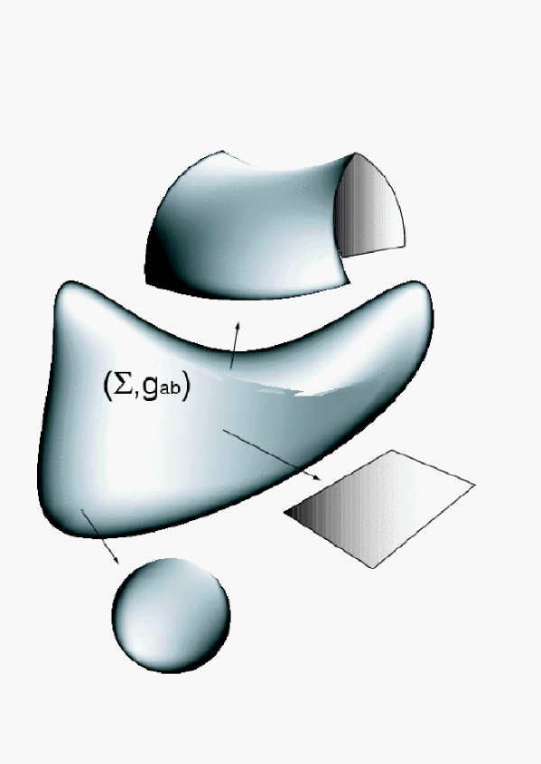
Figure 8: Thurston’s conjecture as viewed by Richard Hamilton is illustrated. The global Ricci flow may have singularities resulting in an effective disconnection of the manifold into “nice” pieces. Thurston’s conjecture assumes that the original manifold can be cut into pieces which themselves have elementary Riemannian structures (associated with the eight “Thurston geometries”). The figure shows three such pieces in a two–dimensional rendering which would correspond to pieces of the three possible FLRW space sections in three dimensions: the $3-$sphere, a piece of a $3-$cylinder, or a piece of a $3-$hyperboloid.

Since, according to Thurston’s geometrization conjecture (Fig. 8), every closed 3–manifold can be decomposed into pieces admitting one of the eight geometric structures mentioned above, it is clear that the global Ricci flow may play a distingushed role in such a conjecture. While such a role clearly motivates the mathematical interest in (52), it also provides a strong argument in favour of (52) as the natural smoothing flow in a regional cosmological averaging procedure. As a matter of fact, the possibility of decomposing a 3–manifold into pieces endowed with a locally homogeneous geometry is particularly appealing to relativistic cosmology, where any such piece may be thought of as representing the regional average of a sufficiently homogeneous portion of the Universe. In such a framework it is suggestive to put the following result by Richard Hamilton into perspective [29] (see also [12]):

Theorem   (Hamilton)

If the closed 3–manifold $(\Sigma,g_{ab})$ admits a non–singular solution $g_{ab}\rightarrow g_{ab}(\beta)$ to (52) for all $0\leq\beta<\infty$, with uniformly bounded sectional curvature, then $(\Sigma,\overline{g}_{ab})$ can be decomposed into pieces admitting one of the following locally homogeneous geometries:

• $(\Sigma,\overline{g}_{ab})$ is a Seifert fibered space.

• $(\Sigma,\overline{g}_{ab})$ is a spherical space form $\mathbb{S}^{3}/\Gamma$.

• $(\Sigma,\overline{g}_{ab})$ is a flat manifold.

• $(\Sigma,\overline{g}_{ab})$ is a constant negative sectional curvature manifold.

• $(\Sigma,\overline{g}_{ab})$ is the union (along incompressible tori) of finite–volume constant negative sectional curvature manifolds and Seifert fibered spaces.

The locally homogeneous geometries $(i)\cdots(v)$ (in particular $(ii)$, $(iii)$, and $(iv)$) are exactly the geometries after which, we believe, the Universe can be regionally modelled after all accidental inhomogeneities are ideally ironed out. Thus, Hamilton’s theorem strongly advocates the basic role of the Ricci flow deformation as a natural mean for averaging locally inhomogeneous 3–geometries in a cosmological setting.

On the cosmological stage, however, we need also to discuss how such a geometrical smoothing flow interacts with the actual distribution of matter.

Combining the Ricci flow and the material mass flow

Our basic idea behind the regional averages $\left\langle\varrho\right\rangle_{B(p;r)}$ is that they replace the local accidental distribution of matter described by $\varrho$. Also, instead of considering just a given geodesic ball $B(p;r_{0})$, we are considering, as $\beta$ varies, a family of geodesic balls $B_{\beta}(p;r_{0})$, all with the same radius $r_{0}$ but with distinct inner geometries $g_{ab}(\beta)$. Note that $r_{0}$ plays here the role of a distance cut–off: it is the typical scale over which we want to smooth the empirical mass distribution. We have to keep track of such a scale in our setup.

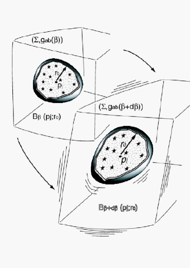
Figure 9: The conservation of the total material mass contained within geodesic ball domains guarantees the comparison of average properties on cosmological mass–scales.

The key idea for obtaining a deformation equation for the regionally averaged mass density field is to fix, besides the scale $r_{0}$ of the Lagrangian ball, also the mass content of the ball under consideration during the deformation process (Fig. 9). It is a physically sensible idea to concentrate on mass scales, since they are only directly related to so–called “comoving” length scales or volumes, respectively [37], if the Eulerian ball is also Euclidean and the inhomogeneites are set up relative to a global reference flow providing the global comoving coordinates.

In order to obtain a deformation equation for the regionally averaged mass density field in the chosen regions $B_{\beta}(p_{j};r_{0})$, we require

$$\frac{\partial}{\partial\beta}M\left(B_{\beta}(p_{j};r_{0})\right)=:\frac{\partial}{\partial\beta}M_{\mathcal{B}_{\beta}}=0$$ (53)

along the solution of (52). Since (the abbreviation $\mathcal{B}_{\beta}:=B_{\beta}(p_{j};r_{0})$ is used hereafter)

$$\left\langle\varrho\right\rangle_{\mathcal{B}_{\beta}}(\beta)=\frac{M_{\mathcal{B}_{\beta}}}{V_{\mathcal{B}_{\beta}}(\beta)}\;,$$ (54)

where $V_{\mathcal{B}_{\beta}}$ denotes the (for each $\beta$ different) volume of the ball in question, it is straightforward to check that we can equivalently rewrite (53) as:

$$\frac{\partial}{\partial\beta}\ln\frac{\left\langle\varrho\right\rangle_{\mathcal{B}_{\beta}}(\beta)}{\left\langle\varrho\right\rangle_{\mathcal{B}_{0}}}+\frac{\partial}{\partial\beta}\ln\frac{V_{\mathcal{B}_{\beta}}(\beta)}{V_{\mathcal{B}_{0}}}\;=\;0\;.$$ (55)

We realize the local rate of volume deformation through the Ricci deformation flow (52) by exploiting the relation:

$$\frac{1}{\sqrt{g(\beta)}}\frac{\partial}{\partial\beta}\sqrt{g(\beta)}=\frac{1}{2}g^{ab}(\beta)\frac{\partial}{\partial\beta}g_{ab}(\beta)=\langle\mathcal{R}(\beta)\rangle_{\Sigma_{\beta}}-\mathcal{R}(\beta)\;,$$ (56)

where $\mathcal{R}(\beta):=g^{ab}(\beta)\mathcal{R}_{ab}(\beta)$ is the scalar curvature associated with $g_{ab}(\beta)$. From this one easily computes that

$$\frac{\partial}{\partial\beta}\ln\frac{V_{\mathcal{B}_{\beta}}(\beta)}{V_{\mathcal{B}_{0}}}\;=\;-\left\langle\mathcal{R}(\beta)\right\rangle_{\mathcal{B}_{\beta}}+\left\langle\mathcal{R}(\beta)\right\rangle_{\Sigma_{\beta}}\;.$$ (57)

Thus we get that the condition of the conservation of the matter content of $B_{\beta}(p_{j};r_{0})$ (53) provides the following $\beta$–evolution for the regionally averaged mass density:

$$\frac{\partial}{\partial\beta}\ln\frac{\left\langle\varrho\right\rangle_{\mathcal{B}_{\beta}}(\beta)}{\left\langle\varrho\right\rangle_{\mathcal{B}_{0}}}\;=\;\left\langle\mathcal{R}(\beta)\right\rangle_{\mathcal{B}_{\beta}}-\left\langle\mathcal{R}(\beta)\right\rangle_{\Sigma_{\beta}}\;.$$ (58)

So far we have established an analogy between matter averaging on different scales and geometrical deformation induced by a suitable flow of metrics. With regard to the constraint equations of general relativity we have to guarantee that this flow of metrics is compatible with the constraints. Before we turn to the problem of smoothing the second fundamental form, it is necessary but also illuminating in what follows to study stability properties of the Ricci flow.

2.2 Stability of the Ricci flow

Associated with the Ricci flow we need to discuss also the properties of the corresponding linearized flow. Roughly speaking, such a necessity comes about since we may be asked what happens to our flow, if the original metric $g_{ab}$, deformed according to $g_{ab}\rightarrow g_{ab}(\beta)$, is slightly perturbed (which is a good question, since the flow is actually perturbed in a dynamical situation, e.g., in the direction of the extrinsic curvature tensor in time $\epsilon=t$):

$$g_{ab}\rightarrow\widehat{g}_{ab}=g_{ab}+\varepsilon h_{ab}\;\;,$$ (59)

where $h_{ab}$ is a symmetric bilinear form, and $\epsilon$ a small parameter. For notational convenience, let us set

$$\mathrm{RF}[g_{ab}(\beta)]:=-2\mathcal{R}_{ab}(\beta)+\frac{2}{3}g_{ab}(\beta)\left\langle\mathcal{R}(\beta)\right\rangle_{\Sigma_{\beta}}\;,$$ (60)

so that the Ricci flow can be compactly written as

$$\frac{\partial}{\partial\beta}g_{ab}(\beta)=\mathrm{RF}[g_{ab}(\beta)]\;\;\;;\;\;\;g_{ab}(\beta=0)=g_{ab}\;.$$ (61)

It is easily checked that, if we perturb the initial metric $g_{ab}(\beta=0)=g_{ab}$, and evolve the perturbed metric $\widehat{g}_{ab}$ according to (52), then we get

$$\widehat{g}_{ab}\rightarrow\widehat{g}_{ab}(\beta)=g_{ab}(\beta)+\varepsilon h_{ab}(\beta)+\mathcal{O}(\varepsilon^{2}),$$ (62)

where $h_{ab}\rightarrow h_{ab}(\beta)$ is a linear flow solution of

$$\frac{\partial}{\partial\beta}h_{ab}(\beta)=D\mathrm{RF}[g_{ab}(\beta)]\circ h_{ab}(\beta):=\frac{d}{d\epsilon}\mathrm{RF}[g_{ab}(\beta)+\varepsilon h_{ab}(\beta)]\Big{|}_{\varepsilon=0}$$

$$h_{ab}(\beta=0)=h_{ab}\;\;.$$ (63)

Explicitly, we obtain (dropping the explicit $\beta$–dependence for notational ease),

$$\frac{\partial}{\partial\beta}h_{ab}=\frac{2}{3}\left\langle\mathcal{R}\right\rangle_{\Sigma_{\beta}}h_{ab}$$

$$+\frac{2}{3}g_{ab}\left[\frac{1}{2}\left\langle\mathcal{R}h_{ik}g^{ik}\right\rangle_{\Sigma_{\beta}}-\frac{1}{2}\left\langle\mathcal{R}\right\rangle_{\Sigma_{\beta}}\left\langle h_{ik}g^{ik}\right\rangle_{\Sigma_{\beta}}-\left\langle\mathcal{R}^{ab}h_{ab}\right\rangle_{\Sigma_{\beta}}\right]$$

$$-\Delta_{L}h_{ab}+2\left[\delta^{\ast}\left(\delta\left(h-\frac{1}{2}(\mathrm{tr}h)g\right)\right)\right]_{ab}\;\;,$$ (64)

where

$$\Delta_{L}h_{ab}:=-\nabla^{s}\nabla_{s}h_{ab}+\mathcal{R}_{as}h_{b}^{s}+\mathcal{R}_{bs}h_{a}^{s}-2\mathcal{R}_{asbt}h^{st}$$ (65)

is the Lichnerowicz–deRham Laplacian on bilinear forms, the operator $\delta$ is (minus) the divergence, and $\delta^{\ast}$ is its formal $L^{2}$–adjoint ( i.e., $1/2$ the Lie derivative operator). All such operators are considered with respect to the $\beta$–varying metric $g_{ab}(\beta)$ of the unperturbed Ricci flow (52). It is clear from its explicit expression that (2.2) takes quite a simpler form, if we restrict our attention to traceless perturbations $h_{ab}$, i.e., if

$$h_{ab}g^{ab}=0\;\;.$$ (66)

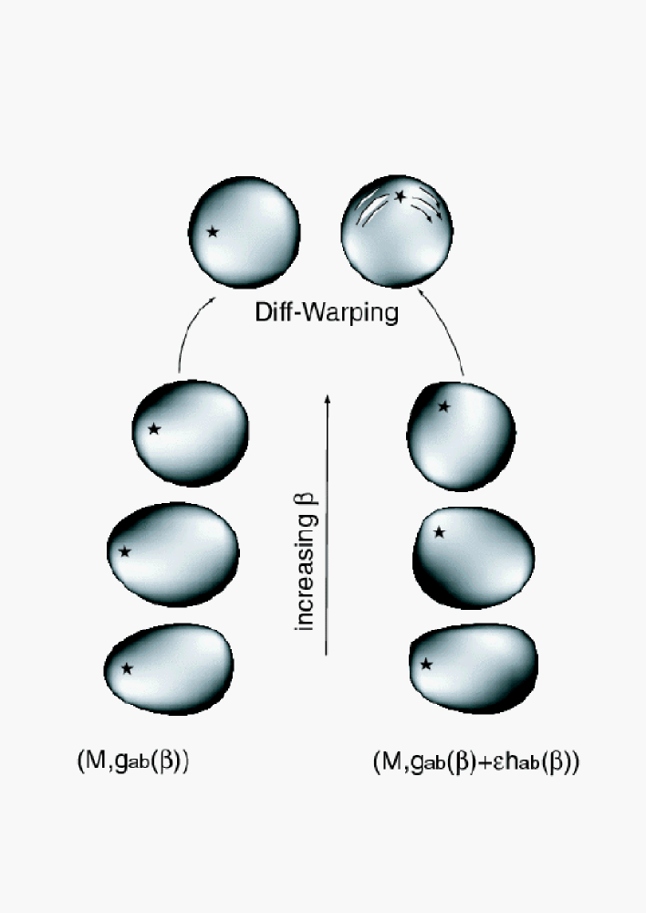
Figure 10: The stability analysis of the Ricci flow under symmetric perturbations allows us to determine the smoothing flow for the second fundamental form. It can be viewed to represent an infinitesimal deformation of metrics connecting two neighboring flows of metrics. The flow of this deformation itself can be shown to be (weakly) parabolic (like the Ricci flow for the metric) up to the infinitesimal equivariance of the Ricci flow under the diffeomorphisms group Diff($\Sigma$) (“Diff–Warping”).

It is then verified that such a condition, if it holds initially (for $\beta=0$), it holds for each value of $\beta$ for which the flows (52) and (2.2) are defined, and we get the much simpler result:

$$\frac{\partial}{\partial\beta}h_{ab}=\frac{2}{3}\left\langle\mathcal{R}\right\rangle_{\Sigma_{\beta}}h_{ab}-\frac{2}{3}g_{ab}\left\langle\mathcal{R}^{ab}h_{ab}\right\rangle_{\Sigma_{\beta}}-\Delta_{L}h_{ab}+{\pounds}_{-\nabla^{k}h_{ik}}g_{ab}\;.$$ (67)

For a given Ricci flow $g_{ab}\rightarrow g_{ab}(\beta)$, Eq. (67) defines a linear (weakly) parabolic initial value problem (the strict parabolicity is broken by the Lie derivative term:

$$\pounds_{-\nabla^{k}h_{ik}}g_{ab}=-\nabla_{a}(\nabla^{k}h_{kb})-\nabla_{b}(\nabla^{k}h_{ka})\;\;,$$ (68)

associated to the infinitesimal equivariance under the diffeomorphisms group $\mathrm{Diff}(\Sigma)$). Given the initial (traceless) perturbation, $h_{ab}(\beta=0)=h_{ab}$, the solution of (67) always exists and is unique, and it represents an infinitesimal deformation of metrics connecting two neighboring flows of metrics $g_{ab}\rightarrow g_{ab}(\beta)$ and $\widehat{g}_{ab}\rightarrow\widehat{g}_{ab}(\beta)$. Since $h_{ab}(\beta)g^{ab}(\beta)=0$, both flows have the same $\beta$ –dependent volume element, i.e.,

$$\sqrt{g(\beta)}=\sqrt{\widehat{g}(\beta)}\;\;,$$ (69)

and thus the same $\beta$–dependent average density $\left\langle\varrho\right\rangle_{\mathcal{B}_{\beta}}$. It is also important to remark that the solution of (67) corresponding to the trivial initial datum (a conformal Lie derivative term $\pounds_{\vec{w}}g_{ab}$),

$$h_{ab}(\beta=0)=\pounds_{\vec{w}}g_{ab}:=\nabla_{a}w_{b}+\nabla_{b}w_{a}-\frac{2}{3}g_{ab}\nabla^{c}w_{c}\;\;,$$ (70)

where $w_{b}$ is a smooth ($\beta$–independent) vector field on $\Sigma$, is provided by

$$h_{ab}(\beta)=\pounds_{\vec{w}}g_{ab}(\beta):=\nabla(\beta)_{a}w_{b}+\nabla(\beta)_{b}w_{a}-\frac{2}{3}g_{ab}(\beta)\nabla(\beta)^{c}w_{c}\;\;,$$ (71)

where the $\beta$–dependence is only through the flow of metrics $g_{ab}\rightarrow g_{ab}(\beta)$ and the associated connection $\nabla_{a}(\beta)$. Such a property is simply a consequence of the $\mathrm{Diff}(\Sigma)$ equivariance of the Ricci flow (Fig. 10). By exploiting such a result, it is possible to prove an important factorization theorem [35] for the structure of the solution $h_{ab}\rightarrow h_{ab}(\beta)$ of (67), which will prove invaluable throughout the rest of the paper, viz.,

Proposition 2   (Lott)

If $h_{ab}\rightarrow h_{ab}(\beta)$ is the flow solution of (67) corresponding to the initial (traceless) datum $h_{ab}(\beta=0)=h_{ab}$, then it can always be factorized according to

$$h_{ab}(\beta)=h_{ab}^{\ast}(\beta)+\pounds_{{\vec{v}}(\beta)}g_{ab}(\beta)\;\;,$$ (72)

where the bilinear form is the solution of the parabolic initial value problem

$$\frac{\partial}{\partial\beta}h_{ab}^{\ast}=-\Delta_{L}h_{ab}^{\ast}+\frac{2}{3}\left\langle\mathcal{R}\right\rangle_{{}_{\Sigma_{\beta}}}h_{ab}^{\ast}-\frac{2}{3}g_{ab}\left\langle\mathcal{R}^{ab}h_{ab}^{\ast}\right\rangle_{{}_{\Sigma(\beta)}},$$ (73)

with $h_{ab}^{\ast}(\beta=0)=h_{ab}$, and where the (now $\beta-$ dependent) vector field $v_{a}(\beta)$ is the flow solution of

$$\frac{\partial}{\partial\beta}v_{a}(\beta)=-\nabla^{c}h_{ac}^{\ast}(\beta)\;\;,\;\;v_{a}(\beta=0)=0\;.$$ (74)

It is appropriate at this point to recall a few relevant facts concerning the geometry behind the structure of the solutions of (67). It follows from the above proposition that, as $\beta\rightarrow\infty$, $h_{ab}(\beta)$ may either approach a (conformal) Lie derivative term $\pounds_{\vec{v}}g_{ab}$, or a non–vanishing deformation tensor $h_{ab}^{\ast}$. This latter non–trivial deformation is only present, if the corresponding Ricci flow $g_{ab}\rightarrow g_{ab}(\beta)$ approaches an Einstein metric on $\Sigma$ which is not isolated (for instance flat tori). In such a case, there is a finite–dimensional manifold of such Einstein metrics, and the non–trivial $h_{ab}^{\ast}$ simply represents infinitesimal deformations connecting two infinitesimally neighboring Einstein metrics on $\Sigma$. As is known, the round metric $\overline{g}_{ab}$ on the three–sphere $\mathbb{S}^{3}$ is isolated in the sense that there are not volume–preserving infinitesimal deformations of $\overline{g}_{ab}$ mapping it to another inequivalent constant curvature metric $\overline{g}_{ab}^{{}^{\prime}}$. In this latter case, (i.e., for isolated constant curvature metrics), as $\beta\rightarrow\infty$, $h_{ab}(\beta)$ must necessarily approach a (conformal) Lie derivative term $\pounds_{\vec{v}}\overline{g}_{ab}$.

2.3 Smoothing the second fundamental form

The properties of the linearized Ricci flow for a traceless metric perturbation $h_{ab}(\beta)$ naturally put to the fore an explicit way for averaging the part of initial data $(\Sigma,g_{ab},K_{ab},\varrho,J_{a})$ related to the second fundamental form $K_{ab}$. One may contend that since $K_{ab}$ carries information on the way $(\Sigma,g_{ab})$ is embedded in the spacetime $(M^{(4)}\simeq\Sigma\times\mathbb{R},g^{(4)})$, one should devise some way of deforming $K_{ab}$ which is independent of the flow of metrics, since this latter flow only depends on the intrinsic geometry of $(\Sigma,g_{ab})$. However, the very geometrical meaning of $K_{ab}$ shows that such a point of view is not correct. According to the evolutive part of the Einstein equations we have:

$$K_{ab}=-\frac{1}{2N}\frac{\partial g_{ab}}{\partial t}+\frac{1}{2N}{\cal L}_{\vec{N}}g_{ab}\;.$$ (75)

Thus, we can write

$$g_{ab}(t)=g_{ab}-t\left[2NK_{ab}-{\cal L}_{\vec{N}}g_{ab}\right]+\mathcal{O}(t^{2})\;\;,$$ (76)

which clearly shows that $2NK_{ab}$ has the natural meaning of the deformation tensor connecting two neighboring Riemannian metrics. If the Ricci flow is the chosen averaging procedure for deforming the metric in the initial data set $(\Sigma,g_{ab},K_{ab},\varrho,J_{a})$, then the stability (under small perturbations) of such a deformation procedure requires that $NK_{ab}$ must necessarily be deformed according to the linearized flow (67 ); there are no other consistent choices.

The only freedom we have concerns which (algebraically independent) part of $K_{ab}$ we want to deform according to (67). From the properties of this latter flow it follows that a smart choice would be to leave undeformed the trace part of $K_{ab}$, and deform only its traceless part (i.e., the associated shear tensor $\sigma_{ab}:=K_{ab}-\frac{1}{3}g_{ab}K$).

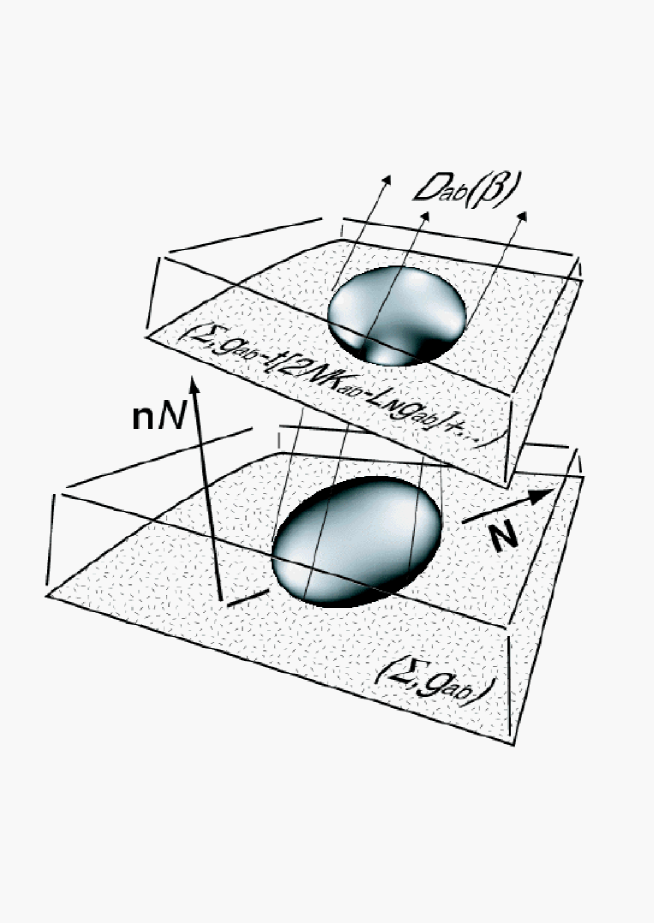
Figure 11: Smoothing the second fundamental form we have the freedom to choose which of the algebraically independent parts of the second fundamental form we wish to smooth out. The trace–free distortion tensor is the natural choice in view of the evolutive part of Einstein’s equations. In the embedding shown in the figure we have assigned the coordinate time to the perturbation parameter $\varepsilon$, and the perturbing symmetric bilinear form was associated with the second fundamental form.

Actually, the geometrical meaning of $K_{ab}$ epitomized by (76) suggests as a more natural choice that we deform the trace–free distortion tensor (Fig. 11):

$$\mathcal{D}_{ab}:=2N\sigma_{ab}-{\pounds}_{\vec{N}}g_{ab}\;\;\;$$

$$\;\;\;\;\;\;=2N\sigma_{ab}\;-\left(\nabla_{a}N_{b}+\nabla_{b}N_{a}-\frac{2}{3}g_{ab}\nabla^{c}N_{c}\right)\;.$$ (77)

In order to $\beta$–deform $\mathcal{D}_{ab}$ in a way consistent with the Ricci flow, let us start observing that, with respect to the metric $g_{ab}$, we can always decompose the given $\mathcal{D}_{ab}$ according to

$$\mathcal{D}_{ab}=\mathcal{D}_{\perp ab}+\mathcal{D}_{\shortparallel ab}$$ (78)

where $\mathcal{D}_{\perp ab}$ is the divergence–free part,

$$\nabla^{a}\mathcal{D}_{\perp ab}=0\;,$$ (79)

and $\mathcal{D}_{\shortparallel ab}$ is the longitudinal part,

$$\mathcal{D}_{\shortparallel ab}={\pounds}_{\vec{w}}g_{ab}\;,$$ (80)

generated by the vector field $\vec{w}$ as a solution of the (elliptic) partial differential equation:

$$\nabla^{a}({\pounds}_{\vec{w}}g_{ab})=\nabla^{a}\left(\nabla_{a}w_{b}+\nabla_{b}w_{a}-\frac{2}{3}g_{ab}\nabla^{c}w_{c}\right)=\nabla^{a}\mathcal{D}_{ab}\;.$$ (81)

Observe further that, according to (76), $\mathcal{D}_{\perp ab}$ represents the part of the distortion tensor that deforms $g_{ab}$ into a nearby distinct Riemannian structure $[g_{ab}(t)]=g_{ab}-\mathcal{D}_{\perp ab}\,t+\mathcal{O}(t^{2})$, whereas $\mathcal{D}_{\shortparallel ab}$ simply generates an infinitesimal ${\rm Diff}(\Sigma)$ reparametrization $g_{ab}\rightarrow g_{ab}-t\left[{\pounds}_{\vec{w}}g_{ab}-{\cal L}_{\vec{N}}g_{ab}\right]+\mathcal{O}(t^{2})$.

With all this in mind, we can apply Lott’s factorization theorem and generate a natural smoothing flow for $\mathcal{D}_{ab}$, $\beta\rightarrow\mathcal{D}_{ab}(\beta)$ as a solution of

$$\frac{\partial}{\partial\beta}\mathcal{D}_{ab}(\beta) = \frac{2}{3}\left\langle\mathcal{R}\right\rangle_{\Sigma_{\beta}}\mathcal{D}_{ab}(\beta)-\frac{2}{3}g_{ab}\left\langle\mathcal{R}^{ab}\mathcal{D}_{ab}(\beta)\right\rangle_{\Sigma_{\beta}}$$ (82)

$$-\Delta_{L}\mathcal{D}_{ab}(\beta)+{\pounds}_{-\nabla^{k}\mathcal{D}_{ik}(\beta)}g_{ab}\;.$$

by setting $\mathcal{D}_{ab}(\beta)=\mathcal{D}_{ab}^{\ast}(\beta)+$ ${\pounds}_{\vec{v}}g_{ab}(\beta)$, where $\mathcal{D}_{ab}^{\ast}(\beta)$ evolves according to the parabolic partial differential equation

$$\frac{\partial}{\partial\beta}\mathcal{D}_{ab}^{\ast}(\beta)=-\Delta_{L}\mathcal{D}_{ab}^{\ast}(\beta)+\frac{2}{3}\left\langle\mathcal{R}\right\rangle_{{}_{\Sigma_{\beta}}}\mathcal{D}_{ab}^{\ast}(\beta)-\frac{2}{3}g_{ab}\left\langle\mathcal{R}^{ab}\mathcal{D}_{ab}^{\ast}(\beta)\right\rangle_{{}_{\Sigma(\beta)}}\;,$$ (83)

with $\mathcal{D}_{ab}^{\ast}(\beta=0)=\mathcal{D}_{ab}$, and where the $\beta-$dependent vector field $v_{a}(\beta)$ is the flow solution of

$$\frac{\partial}{\partial\beta}v_{a}(\beta)=-\nabla^{c}\mathcal{D}_{ac}^{\ast}(\beta)\;\;,\;\;v_{a}(\beta=0)=0\;.$$ (84)

Corresponding to a global solution $\beta\rightarrow g_{ab}(\beta)$ of the Ricci flow, that evolves towards an isolated constant curvature metric $\overline{g}_{ab}=\lim_{\beta\rightarrow+\infty}g_{ab}(\beta)$, the (unique) solution $\beta\rightarrow(\mathcal{D}_{ab}^{\ast}(\beta),v_{a}(\beta))$ of (83), (84) is such that $\overline{\mathcal{D}}_{\perp ab}=\lim_{\beta\rightarrow+\infty}\mathcal{D}_{\perp ab}(\beta)=0$, ($\overline{\mathcal{D}}_{\perp ab}$ will be different from zero only if the constant curvature metric $\overline{g}_{ab}$ is not isolated), and $\overline{\mathcal{D}}_{ab}$ reduces to a pure longitudinal shear, i.e.,

$$\overline{\mathcal{D}}_{ab}=\lim_{\beta\rightarrow+\infty}\mathcal{D}_{ab}(\beta)={\pounds}_{\vec{\widehat{v}}}\overline{g}_{ab}\;,$$ (85)

where

$$\;\widehat{v}_{a}=\lim_{\beta\rightarrow+\infty}v_{a}(\beta)\;\;.$$ (86)

Note that since we can always add to $\mathcal{D}_{ab}(\beta)$ the trivial solution ${\pounds}_{\vec{w}}g_{ab}(\beta)$ of (82), (where the vector field $\vec{w}$ does not depend on $\beta$), by suitably choosing the ($\beta$–independent) vector field ${\vec{w}}$, we can always assume that the conformal Lie derivative term ${\pounds}_{\;\vec{\widehat{v}}}\overline{g}_{ab}$ provided by (85) comprises all the longitudinal shear present in $\overline{\mathcal{D}}_{ab}$.

2.4 The choice of a smoothing reference frame

It is important to stress that the averaging of the trace–free distortion tensor described above implies that we have made a consistent selection for the lapse function $N$, the shift vector field $N_{b}$, and the rate of volume expansion $K$ associated with the given initial data set $(\Sigma,g_{ab},K_{ab},\varrho,J_{a})$. As is well–known, such $(N,N_{b},K)$ are kinematical quantities pertaining to the choice of the initial slice $(\Sigma,g_{ab},\mathcal{D}_{ab})$. They are related also to the choice of the foliation $\Sigma_{t}$ in a suitably small (time) neighborhood of $\Sigma$ in the spacetime resulting from the time–evolution of the data $(\Sigma,g_{ab},K_{ab},\varrho,J_{a})$. Explicity, we have

$$\frac{\partial}{\partial t}K=-\Delta_{g}N+N\left[R+K^{2}-3(4\pi G\rho+\Lambda)\right]+N^{a}\nabla_{a}K\;\;.$$ (87)

This is basically Raychaudhuri’s equation. The rationale underlying the choice of a proper reference frame for carrying out a sensible (regional) averaging, is that (87) should reflect the achieved regularity in the averaged geometry and matter fields, without introducing frame–dependent inhomogeneities and anisotropies. This implies that, as we $\beta$–deform the local inhomogeneities and anisotropies of $(\Sigma,g_{ab},\mathcal{D}_{ab})$, we need also to eliminate the inhomogeneous artifacts due to the choice of the slicing associated with $(\Sigma,N,N_{b},K)$. To give an example, it is often argued that a good candidate for supporting an “almost–Friedmannian” initial data set $(\Sigma,g_{ab},K_{ab})$ is the surface of constant matter density in the cosmic fluid frame, or the surface of constant 4–velocity potential ([24], [23], [4], [5], [19], [16], [7]). The point is that in such a slicing a slightly perturbed model features an almost constant lapse function, since the instantaneous acceleration for such a frame of reference is observationally quite small. The observed expansion and shear are also small. In line of principle these remarks suggest that a set $(\Sigma,N,N_{b},K)$ characterized in this way is, in the observed domain, the most suitable one for implementing an averaging procedure. At any rate, even for such a natural and almost optimal choice of $(\Sigma,N,N_{b},K)$, we still have the issue of how to consistently get rid of the (residual) frame fluctuations present in $N$, $N_{b}$, and $K$. In order to eliminate such fluctuations, both the lapse function $N(\beta)$, the shift vector field $N_{a}(\beta)$, and the rate of volume expansion $K(\beta)$ are to be considered as explicitly $\beta-$dependent, (taking the given values $(N,N_{b},K)$ for $\beta=0$). In other words, we need to consider on $(\Sigma,g_{ab},\mathcal{D}_{ab})$ a one–parameter ($\beta$) family of (instantaneous) frames of reference $(\Sigma,N(\beta),N_{b}(\beta))$ and devise a way for characterizing their $\beta$–evolution. The rationale is to end up in a frame which, for $\beta\rightarrow\infty$, reflects, as much as possible, the homogeneous and isotropic properties of the geometry resulting from the $\beta$ –evolution of $(\Sigma,g_{ab},\mathcal{D}_{ab})$. Such a frame will correspond to the standard Friedmannian scenario of use in cosmology.

A word of caution is mandatory here. In mathematical cosmology it is often the case that the choice of foliation is strictly connected to the structure of the constraint equations via the use of $K$ as the variable conjugated to time (York’s extrinsic time). Spatially constant $K$ is then a rather popular choice. However, the rate of volume expansion plays a distinguished dynamical role in Friedmannian cosmology, and for our purposes it would be quite detrimental to use $K$ as the variable selecting the hypersurface $\Sigma$ carrying the data to be averaged. In line of principle, the structure of the Ricci flow suggests that one should pick up a $\Sigma$ such that $(\Sigma,g_{ab})$ admits a global $0\leq\beta<\infty$ Ricci flow, for instance this is the case if the Ricci tensor of $(\Sigma,g_{ab})$ is positive or (hopefully!) not too wildly oscillating. However, this is again something which is under control of mathematics, but not acceptable for the physical situation; it cannot be used as a viable selection criterium. The best we can hope for is to assume that $\Sigma$ is ideally chosen among the $t$–constant slices of a global frame of reference where, for scales sufficiently larger than the relevant averaging scale, the distant galaxies appear to recede radially. And, as argued before, such a $\Sigma$ may be appropriately realized, e.g., by the surface of constant matter density in the cosmic fluid frame.

The lapse function

We postpone to the next section the issue of the $\beta$–evolution of the rate of volume expansion $K$, since this latter is strictly connected to the regional averaging of the constraints. On the other hand, for the $\beta$ –evolution of the kinematical variables $(N,N_{b})$ there are physically sound choices which are directly suggested by the nature of the Raychaudhuri equation, and from the structure of the equations (83), and (84). To start with, let us observe that since the leading lapse–dependent inhomogeneity inducing term in (87) is $\Delta_{g}N$ it is natural to smooth the lapse function $N$ by diffusing its inhomogeneities by means of the scalar heat equation:

$$\frac{\partial}{\partial\beta}N(\beta)=\Delta_{g(\beta)}N(\beta)\;\;\;;\;\;\;N(\beta=0)=N\;\;,$$ (88)

where $\Delta_{g(\beta)}$ is the Laplacian of the metric $g_{ab}(\beta)$ evolved by the Ricci flow. This is basically the harmonic map flow for the map $N(\beta):\Sigma\rightarrow\mathbb{R}$. Note also that this is a non–uniformly parabolic initial value problem, because $\Delta_{g(\beta)}$ depends on the $\beta$–varying metric $g_{ab}(\beta)$. Let us assume that, for $\beta=0$, the given lapse function is such that $0<\varepsilon\leq N\leq C_{1}$, $\left|\nabla N(\beta=0)\right|\leq C_{2}$, where $C_{1}$ and $C_{2}$ are suitable constants. In other words, the (instantaneous) acceleration $\nabla_{a}\ln N$ of the frame associated with the chosen slice $\Sigma$ is assumed to be bounded. Then, according to the maximum principle for (88) (e.g. see [1]), we have $0<\varepsilon\leq N(\beta)\leq C_{1}$, $\left|\nabla N(\beta)\right|\leq C_{2}$ for $\beta\geq 0$. If the Ricci flow exists for all $\beta\geq 0$, then by looking at the $\beta$–evolution of $\left|\nabla N(\beta)\right|^{2}=g^{ab}(\beta)\nabla_{a}N(\beta)\nabla_{b}N(\beta)$, a long but elementary computation provides:

$$\frac{\partial}{\partial\beta}\left|\nabla N(\beta)\right|^{2}$$

$$=\Delta_{g(\beta)}\left(\left|\nabla N(\beta)\right|^{2}\right)-2\left|\nabla^{2}N(\beta)\right|^{2}+\nabla^{a}N\nabla^{b}N\left(\frac{\partial}{\partial\beta}g_{ab}(\beta)+2{\cal R}_{ab}\right)\;\;,$$ (89)

which shows that, if we deform the metric along the Ricci flow, then we have:

$$\frac{\partial}{\partial\beta}\left|\nabla N(\beta)\right|^{2}=\Delta_{g(\beta)}\left(\left|\nabla N(\beta)\right|^{2}\right)-2\left|\nabla^{2}N(\beta)\right|^{2}-\frac{2}{3}\left|\nabla N(\beta)\right|^{2}\left\langle\mathcal{R}\right\rangle_{\Sigma_{\beta}}\;\;.$$ (90)

It follows that the maximum of $\left|\nabla N(\beta)\right|^{2}$ is weakly monotonically decreasing as $\beta\rightarrow\infty$; (the apparent condition for this to occur is $\left\langle\mathcal{R}\right\rangle_{\Sigma_{\beta}}\geq 0$, but this condition is actually not necessary, as can be seen by rescaling the $\beta-$variable to the standard unnormalized Ricci flow). Parabolic theory shows that, if the Ricci flow is global (with uniformly bounded curvature), then also $\beta\rightarrow N(\beta)$ exists for all $\beta$ and $\left|\nabla N(\beta)\right|\rightarrow 0$ as $\beta\rightarrow\infty$. Physically, such an averaging procedure implies that the frame instantaneous acceleration associated with the chosen slice $\Sigma$ is smoothly damped, and up to a normalization we can assume that as $\beta\rightarrow\infty$, $N(\beta)\rightarrow 1$ uniformly. Note that if one identifies $\Sigma$ with a surface of constant matter density or constant $4-$velocity potential, respectively, in the frame of reference comoving with the flow lines of the (irrotational) cosmic fluid, then an inhomogeneous $N$ can be directly related to the instantaneous acceleration of the fluid particles on $\Sigma$, thus $N(\beta)\rightarrow 1$ as $\beta\rightarrow\infty$ implies that the fluid particles are, on $\Sigma$, in free fall.

The shift vector and the matter current density

Since $N_{a}$ generates local diffeomorphisms in the hypersurface $\Sigma$, a procedure for smoothly averaging out the shift vector field $N_{a}$ cannot be disentangled from the averaging of the matter current density $J_{a}$ and from the fact that the averaging of the distortion tensor $\mathcal{D}_{ab}(\beta)$ generates, according to Lott’s factorization theorem, a geometrically induced shift $v_{a}(\beta)$ (see (84)). Along the same lines of the above remarks one may tentatively assume that $N_{a}$ can be related to the local $3$–velocities of the fluid particles on $\Sigma$. On a sufficiently large cosmic domain we may put ourselves initially on $\Sigma$ (i.e., for $\beta=0$) into a frame with vanishing shift: $N_{a}=0=J_{a}$. Naively, one would expect that such a situation will persist as we deform the data $(\Sigma,g_{ab},\mathcal{D}_{ab})$. However, as already stressed, there is a diffeomorphism warp generated by the linearized Ricci flow, which, if not properly taken into account, will manifest itself as a current $J_{a}$ of the matter on the smoothed data $(\Sigma,g_{ab}(\beta),\mathcal{D}_{ab}(\beta))$ when $\beta\rightarrow\infty$. The physical origin of such diff–induced matter current is rather easy to understand. Roughly speaking, what happens is that the points of the manifold $\Sigma$ are moved around as curvature bumps are ironed out, (the generator of such a motion is the gradient in scalar curvature $\nabla_{a}{\cal R}$; these are basically the Diff–solitons familiar in the Ricci flow theory). From a Lagrangian point of view, this motion is transferred to the fluid particles labelled by the corresponding points of $\Sigma$.

Thus, in order to consistently compensate for such a Ricci flow induced warping, we must assume that for $\beta\geq 0$ we have a non–vanishing shift $N_{a}(\beta)$ and a corresponding matter current density $J_{a}(\beta)$. The natural choice that suggests itself is to introduce a $\beta$ –dependent shift $\beta\rightarrow N_{a}(\beta)$, according to

$$N_{a}(\beta)=\widehat{v}_{a}-v_{a}(\beta)\;\;,$$ (91)

where $v_{a}(\beta)$ is the flow solution of (84), and $\widehat{v}_{a}$ is its $\beta\rightarrow\infty$ limiting value given by (86). Note that, according to such a choice,

$$N_{a}(\beta=0)=\widehat{v}_{a}\;,\quad N_{a}(\beta\rightarrow\infty)=0\;\;,$$ (92)

so that the shift $N_{a}(\beta)$ exactly balances the longitudinal shear ${\pounds}_{v}g_{ab}(\beta)$ generated by the (linearized) Ricci flow for $0\leq\beta<\infty$. In other words, there is an optimal choice $\widehat{v}_{a}$ for the $3$–velocity field of the instantaneous observers on $\Sigma$ which allow them to isotropically smooth the data $(\Sigma,g_{ab},\mathcal{D}_{ab})$. If we, e.g., identify $\Sigma$ with a surface of constant average matter density $\left\langle\varrho\right\rangle_{\mathcal{B}_{\beta}}$, then the Ricci flow induced shift $\beta\rightarrow N_{a}(\beta)$ gives rise to a fictious material convection current density $\beta\rightarrow J_{a}(\beta)$ given by

$$J_{a}(\beta):=\left\langle\varrho\right\rangle_{\mathcal{B}_{\beta}}N_{a}(\beta)\;\;,$$ (93)

where $\left\langle\varrho\right\rangle_{\mathcal{B}_{\beta}}$ is the averaged matter density over the region of interest, (see (58)). Observe that $J_{a}(\beta)\rightarrow 0$ uniformly as $\beta\rightarrow\infty$.

2.5 Constraints on regional averaging

We are now going to study the asymptotic properties of the variables under the Lagrangian smoothing flows as $\beta\rightarrow\infty$. For this purpose we have to go first into the constraint equations in order to establish a link between the actual and the regionally smoothed–out initial data.

The constraint equations

If we are willing to assume that Einstein’s equations hold on the regions $B_{\beta}(p_{j};r_{0})$ where we are averaging, then besides the integral constraint of regional mass preservation, we must also require that our regional averaging procedure is such as to respect the constraints Eqs. (3), at least on the given scale $r_{0}$. Thus, we restrict the class of possible deformation flows to act within the solution space of the constraints. In other words, for each $\beta$ the smoothed geometry should be a candidate for an admissible initial data set of Einstein’s equations in $B_{\beta}(p_{j};r_{0})$.

The divergence constraint

Let us start by discussing the divergence constraint, which, in terms of the trace–free distortion tensor $\mathcal{D}_{ab}$ reads:

$$\nabla^{b}\left[\frac{1}{2N}\mathcal{D}_{ab}+\frac{1}{2N}{\pounds}_{\vec{N}}g_{ab}\right]-\frac{2}{3}\nabla_{a}K=8\pi G\,J_{a}\;\;,$$ (94)

or more explicitly

$$\frac{1}{2N}\left[\nabla^{b}\left(\mathcal{D}_{ab}+{\pounds}_{\vec{N}}g_{ab}\right)-\left(\mathcal{D}_{ab}+{\pounds}_{\vec{N}}g_{ab}\right)\nabla^{b}\ln N\right]-\frac{2}{3}\nabla_{a}K=8\pi G\,J_{a}\;\;.$$ (95)

If we assume that such a constraint holds in the regions $B_{\beta}(p_{j};r_{0})$ also for the $\beta$–deformed distortion tensor $\mathcal{D}_{ab}(\beta)$ we formally get:

$$\frac{1}{2N(\beta)}\left[\nabla^{b}\left(\mathcal{D}_{ab}^{\ast}+{\pounds}_{\vec{N}+\vec{v}}g_{ab}\right)-\left(\mathcal{D}_{ab}^{\ast}+{\pounds}_{\vec{N}+\vec{v}}g_{ab}\right)\nabla^{b}\ln N\right]_{\beta}$$

$$-\frac{2}{3}\nabla_{a}K(\beta)\;=\;8\pi G\,J_{a}(\beta)\;\;,$$ (96)

where the notation $[....]_{\beta}$ is a shorthand for the explicit $\beta$–dependence of all the quantities within the brackets.

According to the choice (91) for the $\beta$–dependent shift vector field $N_{a}(\beta)$, (2.5) reduces to

$$\frac{1}{2N(\beta)}\left[\nabla^{b}\left(\mathcal{D}_{ab}^{\ast}+{\pounds}_{\widehat{v}}g_{ab}\right)-\left(\mathcal{D}_{ab}^{\ast}+{\pounds}_{\widehat{v}}g_{ab}\right)\nabla^{b}\ln N\right]_{\beta}$$

$$-\frac{2}{3}\nabla_{a}K(\beta)=8\pi G\,J_{a}(\beta)\;,$$ (97)

where the matter current $J_{a}(\beta)$ is given by (93).

Assuming that the smoothing flow $\beta\rightarrow(g_{ab}(\beta),\mathcal{D}_{ab}^{\ast}(\beta),v_{a}(\beta))$ is global and that $g_{ab}(\beta)\rightarrow\overline{g}_{ab}$ is an isolated constant curvature metric, then $\mathcal{D}_{ab}^{\ast}(\beta)\rightarrow 0$, $\nabla^{b}\ln N\rightarrow 0$ , and $J_{a}(\beta)\rightarrow 0$, uniformly, and (2.5) reduces to

$$\overline{\nabla}^{b}\left({\pounds}_{\widehat{v}}\overline{g}_{ab}\right)-\frac{2}{3}\partial_{a}\overline{K}=0\;\;,$$ (98)

where $\overline{A}$ is the $\beta\rightarrow\infty$ limiting value of the given quantity $A$. Thus, the possible anisotropies in the gradient of the rate of volume expansion $\overline{K}$, as seen by the observers executing the smoothing process in $B_{\beta}(p_{j};r_{0})$, are only due to the diff–warp generated by the Ricci flow.

The Hamiltonian constraint

We are now in position of discussing the Hamiltonian constraint. By adopting the same regional philosophy applied to the divergence constraint, we assume that it holds in $B_{\beta}(p_{j};r_{0})$ for the $\beta$–dependent data on $(\Sigma_{\beta},g_{ab}(\beta))$. Explicitly, in terms of the trace–free distortion tensor $\mathcal{D}_{ab}$, we get:

$$\mathcal{R}(\beta)+\frac{2}{3}K^{2}(\beta)$$

$$-\frac{1}{4N^{2}(\beta)}g^{ab}(\beta)g^{cd}(\beta)\left[\mathcal{D}_{ac}^{\ast}+{\pounds}_{\vec{N}+\vec{v}}g_{ac}\right]_{\beta}\left[\mathcal{D}_{bd}^{\ast}+{\pounds}_{\vec{N}+\vec{v}}g_{bd}\right]_{\beta}$$

$$=\;16\pi G\rho(\beta)+2\Lambda\;\;.$$ (99)

According to (91) this reduces to

$$\mathcal{R}(\beta)+\frac{2}{3}K^{2}(\beta)-\frac{1}{4N^{2}(\beta)}g^{ab}(\beta)g^{cd}(\beta)\left[\mathcal{D}_{ac}^{\ast}+{\pounds}_{\widehat{v}}g_{ac}\right]_{\beta}\left[\mathcal{D}_{bd}^{\ast}+{\pounds}_{\widehat{v}}g_{bd}\right]_{\beta}$$

$$=\;16\pi G\rho(\beta)+2\Lambda\;,$$ (100)

which, upon taking the volume–average over $B_{\beta}(p_{j};r_{0})$, yields:

$$\left\langle\mathcal{R}(\beta)\right\rangle_{\mathcal{B}_{\beta}}+\frac{2}{3}\left\langle K^{2}(\beta)\right\rangle_{\mathcal{B}_{\beta}}$$

$$-\frac{1}{4}\left\langle\frac{g^{ab}(\beta)g^{cd}(\beta)\left[\mathcal{D}_{ac}^{\ast}+{\pounds}_{\widehat{v}}g_{ac}\right]_{\beta}\left[\mathcal{D}_{bd}^{\ast}+{\pounds}_{\widehat{v}}g_{bd}\right]_{\beta}}{N^{2}(\beta)}\right\rangle_{\mathcal{B}_{\beta}}$$

$$=\;16\pi G\left\langle\mathcal{\rho}(\beta)\right\rangle_{\mathcal{B}_{\beta}}+2\Lambda\;\;.$$ (101)

According to (58) we have:

$$\left\langle\mathcal{\rho}(\beta)\right\rangle_{\mathcal{B}_{\beta}}=\left\langle\mathcal{\rho}\right\rangle_{\mathcal{B}_{0}}e^{\int_{0}^{\beta}\left[\left\langle\mathcal{R}(\lambda)\right\rangle_{\mathcal{B}_{\lambda}}-\left\langle\mathcal{R}(\lambda)\right\rangle_{\Sigma_{\lambda}}\right]d\lambda}\;\;.$$ (102)

Since, in the $\beta\rightarrow\infty$ limit $\mathcal{D}_{bd}^{\ast}(\beta)\rightarrow 0$, $N(\beta)\rightarrow 1$ uniformly (again by assuming that the Ricci flow metric $g_{ab}(\beta)\rightarrow\overline{g}_{ab}$ is an isolated constant curvature metric), we can write (2.5) as:

$$\left\langle\overline{\mathcal{R}}\right\rangle_{\overline{\mathcal{B}}}+\frac{2}{3}\left\langle\overline{K}^{2}\right\rangle_{\overline{\mathcal{B}}}$$

$$=\;16\pi G\left\langle\mathcal{\rho}\right\rangle_{\mathcal{B}_{0}}e^{\int_{0}^{\infty}\left[\left\langle\mathcal{R}(\beta)\right\rangle_{\mathcal{B}_{\beta}}-\left\langle\mathcal{R}(\beta)\right\rangle_{\Sigma_{\beta}}\right]d\beta}+\frac{1}{4}\left\langle\overline{g}^{ab}\overline{g}^{cd}{\pounds}_{\widehat{v}}\overline{g}_{ac}{\pounds}_{\widehat{v}}\overline{g}_{bd}\right\rangle_{\overline{\mathcal{B}}}+2\Lambda\;\;.$$ (103)

Observe that

$$\frac{1}{4}\left\langle\overline{g}^{ab}\overline{g}^{cd}{\pounds}_{\widehat{v}}\overline{g}_{ac}{\pounds}_{\widehat{v}}\overline{g}_{bd}\right\rangle_{\overline{\mathcal{B}}}=2\left\langle\overline{\sigma}^{2}\right\rangle_{\overline{\mathcal{B}}}\;\;,$$ (104)

where $\overline{\sigma}^{2}=\frac{1}{2}\overline{\sigma}_{ab}\overline{\sigma}^{ab}$ is the squared norm of the shear tensor. Moreover, since $\overline{g}_{ab}$ is a constant curvature metric, $\overline{\mathcal{R}}$ is a constant that, in order to emphasize the regional nature of the averaging, we denote by $\overline{\mathcal{R}}_{\overline{\mathcal{B}}}$. Thus, we finally get:

$$\frac{2}{3}\left\langle\overline{K}^{2}\right\rangle_{\overline{\mathcal{B}}}=16\pi G\left\langle\mathcal{\rho}\right\rangle_{\mathcal{B}_{0}}e^{\int_{0}^{\infty}\left[\left\langle\mathcal{R}(\beta)\right\rangle_{\mathcal{B}_{\beta}}-\left\langle\mathcal{R}(\beta)\right\rangle_{\Sigma_{\beta}}\right]d\beta}+2\left\langle\overline{\sigma}^{2}\right\rangle_{\overline{\mathcal{B}}}+2\Lambda-\overline{\mathcal{R}}_{\overline{\mathcal{B}}}\;\;.$$ (105)

2.6 Summary of key–results

Before we discuss cosmological implications, we here summarize the key–results of the previous sections that are relevant for applications.

In Section 1 we have introduced the concept of a (position–dependent) system of geodesic ball–domains on which volume–averages of scalar functions are evaluated. We have explicitly shown how the averaged density of matter and the geometry of balls change under variation of scale. Complementary to this (Eulerian) averaging under variation of the ball radius, we have devised a (Lagrangian) smoothing flow that provides a conceptually equivalent averaging procedure. Here, we gave substance to the choice of the Ricci flow as a natural candidate for the smoothing of the metric. The key–results of this section were:

• For scalar functions on a Riemannian 3–manifold the operations spatial averaging and rescaling the domain of averaging do not commute. In particular, this shows that averaging of (scalar) inhomogeneous fields implies the necessity of simultaneously rescaling the (tensorial) geometry.

• The metric in the neighborhood of the domain of averaging is forced to rescale in the direction of its Ricci tensor.

Important equations were Eq. (44) (Proposition 1) and Eq. (33) in the context of (Eulerian) averaging under variation of the ball radius, and the corresponding equations in the context of (Lagrangian) smoothing, Eq. (47) and Eq. (48).

In Section 2 we have put into practice the smoothing program in terms of a globally volume–preserving Ricci deformation flow. We stressed that the choice of this global normalization is technical, the key–results concerning regional averages do not depend on this choice. We devised a corresponding deformation flow for the material mass under the assumption that the total material mass within the domain of averaging is preserved during the deformation. We then showed that the stability properties of the Ricci flow entail a unique choice of the smoothing flow for the second fundamental form. We implemented the requirement of the preservation of the constraints under such deformations, and determined the optimal choice for the reference frame in which fundamental observers execute the smoothing procedure. The key–results of this section were:

• The Ricci flow for the metric and the corresponding material mass flow link the global and regional averages for the material mass density and the scalar curvature.

• The second fundamental form must necessarily be deformed according to the linearized Ricci flow; there are no other consistent choices.

• The optimal choice of the smoothing reference frame is determined by compensating for the fictious motion of fundamental observers that is induced by the geometrical deformation.

• To get a consistent picture, the constraint equations were required to be preserved during the smoothing procedure, i.e., the smoothing flows were required to act within the solution space of Einstein’s equations.

Important equations were Eq. (52), Eq. (54) and Eq. (58) for the Ricci– and material mass flows, and Eq. (67) together with Proposition 2 for the linearized Ricci flow in connection with the smoothing of the second fundamental form. Instead of smoothing the second fundamental form, smoothing of the trace–free distortion tensor was suggested, Eq. (77). Eq. (88) and Eq. (91) determine the smoothing of the lapse function and shift vector, respectively. As for the constraints we note that, while the momentum constraint was of technical importance concerning the consistency of our choice of smoothing the shift vector field, Eq. (2.5), (remember that the shift vector field cannot be disentangled from the averaging of the matter current density, and the averaging of the distortion tensor $\mathcal{D}_{ab}(\beta)$ generates, according to Lott’s factorization theorem, a geometrically induced shift), the Hamiltonian constraint is essential for the following applications, so we especially point out Eq. (2.5) and Eq. (105).

In the next section we are going to discuss average characteristics in the smoothed–out region. In particular, we shall discuss the effect of averaging and scaling, respectively, on the parameters of an averaged inhomogeneous cosmology with the key result:

• Cosmological parameters, as they are interpreted in a smoothed cosmology, are ‘dressed’ by the removed geometrical inhomogeneities.

Important equations will be Eq. (118) together with Eq. (119) featuring a novel “curvature backreaction” effect; Eq. (120) as compared to Eq. (126) for generalizations of Friedmann’s equation in the actual cosmological model and the smoothed model, respectively. The Hamiltonian constraint may be cast into a constraint equation for regional cosmological parameters in the actual model (Eq. (125)) and the smoothed model (Eq. (129)), which lie at the basis of our interpretation concerning ‘bare’ and ‘dressed’ cosmological parameters.

3 Cosmological Implications

We are now going to study Eq. (105) in a cosmological setting, addressing especially the role of the cosmological parameters. Before we discuss them, let us first study and estimate the fluctuations in the rate of expansion and the scalar curvature.

3.1 Estimating fluctuations

In order to write (105) in a form suggesting a generalized Friedmann equation, let us first introduce the regional variance of the distribution of $\overline{K}$ in $\overline{\cal B}(p_{j};r_{0})$ measuring the spatial fluctuations in the rate of expansion:

$$\delta_{\overline{K}}^{2}:=\left\langle\left(\overline{K}-\left\langle\overline{K}\right\rangle_{\overline{\mathcal{B}}}\right)^{2}\right\rangle_{\overline{\mathcal{B}}}=\left\langle\overline{K}^{2}\right\rangle_{\overline{\mathcal{B}}}-\left\langle\overline{K}\right\rangle_{\overline{\mathcal{B}}}^{2}\;\;.$$ (106)

The second step is to exploit (98) in order to get an estimate for $\delta_{\overline{K}}^{2}$ in $\overline{\cal B}(p_{j};r_{0})$. Note that the following estimates are just indicative for the sake of understanding; we shall comment on strategies for full estimates later.

Recall that for any ($C^{2}$) function on $\overline{\cal B}(p_{j};r_{0})$ we can write (as long as ${\cal R}(p_{j})r_{0}^{2}\ll 1$):

$$\frac{1}{V_{E}r_{0}^{3}}\int_{\overline{\cal B}(p_{j};r_{0})}f\;d\mu_{\overline{g}}=f(p_{j})+\frac{r_{0}^{2}}{10}\left[\Delta f(p_{j})-\frac{\overline{\mathcal{R}}_{\overline{\mathcal{B}}}}{3}f(p_{j})\right]+o(r_{0}^{2})\;\;,$$ (107)

where $V_{E}$ is the Euclidean volume of the unit ball in $\mathbb{R}^{3}$, and $\Delta$ is the Euclidean Laplacian. Upon applying such a normal coordinates estimate to $f=\overline{K}^{2}$ and $f=\overline{K}$, we obtain for the fluctuations of the rate of expansion:

$$\delta_{\overline{K}}^{2}=\frac{r_{0}^{2}}{10}\left[2\left(\delta^{ab}\partial_{a}\overline{K}\partial_{b}\overline{K}\right)(p_{j})+\frac{\overline{\mathcal{R}}_{\overline{\mathcal{B}}}}{3}\overline{K}^{2}(p_{j})\right]+o(r_{0}^{2})\;\;,$$ (108)

which, upon substituting the expression (98) for $\partial_{a}\overline{K}$, yields:

$$\delta_{\overline{K}}^{2}=\frac{r_{0}^{2}}{10}\left[\frac{9}{2}\left(\delta^{ab}\nabla^{c}\overline{\sigma_{\shortparallel}}_{ac}\nabla^{d}\overline{\sigma_{\shortparallel}}_{bd}\right)(p_{j})+\frac{\overline{\mathcal{R}}_{\overline{\mathcal{B}}}}{3}\overline{K}^{2}(p_{j})\right]+o(r_{0}^{2})\;\;,$$ (109)

where $\overline{\sigma_{\shortparallel}}_{ac}={\pounds}_{\widehat{v}}\overline{g}_{ac}$ is the residual longitudinal shear.

Inserting (57) into the integral of (58) we also get:

$$\left\langle\mathcal{\rho}\right\rangle_{\mathcal{B}_{0}}e^{\int_{0}^{\infty}\left[\left\langle\mathcal{R}(\beta)\right\rangle_{\mathcal{B}_{\beta}}-\left\langle\mathcal{R}(\beta)\right\rangle_{\Sigma_{\beta}}\right]d\beta}=\left\langle\mathcal{\rho}\right\rangle_{\mathcal{B}_{0}}\frac{V_{\mathcal{B}_{\beta}}(\beta=0)}{V_{\mathcal{B}_{\beta}}(\beta\rightarrow\infty)}=\left\langle\mathcal{\rho}\right\rangle_{\mathcal{B}_{0}}\frac{V_{\mathcal{B}_{0}}}{V_{\overline{\mathcal{B}}}}=\left\langle\mathcal{\rho}\right\rangle_{\overline{\mathcal{B}}}\;.$$ (110)

A normal coordinates estimate as in (107) (set $f\equiv 1$) explicitly provides:

$$\left\langle\mathcal{\rho}\right\rangle_{\mathcal{B}_{0}}=\left\langle\mathcal{\rho}\right\rangle_{\overline{\mathcal{B}}}\frac{1-\frac{1}{30}\overline{\mathcal{R}}_{\overline{\mathcal{B}}}r_{0}^{2}}{1-\frac{1}{30}\mathcal{R}_{\overline{\mathcal{B}}}(p_{j})r_{0}^{2}}+o(r_{0}^{2})\;,$$ (111)

revealing the actual dependence of $\left\langle\mathcal{\rho}\right\rangle_{\mathcal{B}_{0}}$ on the local curvature $\mathcal{R}_{\overline{\mathcal{B}}}(p_{j})$ with respect to the regional average curvature $\overline{\mathcal{R}}_{\overline{\mathcal{B}}}$. In this connection, it is also worthwhile to discuss how the regional curvature in the smoothed region $\overline{\mathcal{R}}_{\overline{\mathcal{B}}}$ is related to the actual average curvature $\left\langle\mathcal{R}\right\rangle_{\mathcal{B}_{0}}$.

Let us start by noting that the (normalized) $\beta-$evolution of the scalar curvature obeys the following equation [1], [28]:

$$\frac{\partial{\cal R}(\beta)}{\partial\beta}=\Delta_{g(\beta)}{\cal R}(\beta)+2{\cal W}(\beta)-\frac{2}{3}{\cal R}(\beta)\left\langle{\cal R}(\beta)\right\rangle_{\Sigma_{\beta}}\;\;,$$ (112)

where we have defined

$${\cal W}(\beta):=\;g^{ab}g^{cd}{\cal R}_{ac}(\beta){\cal R}_{bd}(\beta)$$

$$=\;g^{ab}g^{cd}[{\tilde{\cal R}}_{ac}+\frac{1}{3}g_{ac}{\cal R}][{\tilde{\cal R}}_{bd}+\frac{1}{3}g_{bd}{\cal R}]={\tilde{\cal R}}^{ab}{\tilde{\cal R}}_{ab}+\frac{1}{3}{\cal R}^{2}\;.$$ (113)

A straightforward calculation then provides:

$$\frac{\partial}{\partial\beta}\langle{\cal R}(\beta)\rangle_{{\cal B}_{\beta}}=\frac{1}{V_{{\cal B}_{\beta}}}\int_{\partial{\cal B}_{\beta}}\nabla_{a}{\cal R}(\beta)\;d\sigma^{a}_{g(\beta)}\;\;+\;2\langle{\tilde{\cal R}}^{ab}(\beta){\tilde{\cal R}}_{ab}(\beta)\rangle_{{\cal B}_{\beta}}$$

$$-\frac{1}{3}\langle\left({\cal R}(\beta)-\langle{\cal R}(\beta)\rangle_{{\cal B}_{\beta}}\right)^{2}\rangle_{{\cal B}_{\beta}}+\frac{2}{3}\langle{\cal R}(\beta)\rangle_{{\cal B}_{\beta}}\left(\langle{\cal R}(\beta)\rangle_{{\cal B}_{\beta}}-\langle{\cal R}(\beta)\rangle_{\Sigma_{\beta}}\right)\;.$$ (114)

On the closed manifold $\Sigma$, i.e., taking ${\cal B}_{\beta}\;\rightarrow\;\Sigma_{\beta}$, the first term on the r.h.s. of Eq. (3.1) reduces to a flux through an empty boundary and the last term, specifying the deviation from the regional to the global average curvature, vanishes, and Eq. (3.1) may be integrated to yield:

$$\overline{\mathcal{R}}_{\Sigma_{\beta\rightarrow\infty}}=\left\langle\mathcal{R}\right\rangle_{\Sigma_{\beta=0}}+\int_{0}^{\infty}\left[2\left\langle\widetilde{\cal R}^{ab}\widetilde{\cal R}_{ab}\right\rangle_{\Sigma_{\beta}}-\frac{1}{3}\left(\left\langle\mathcal{R}^{2}\right\rangle_{\Sigma_{\beta}}-\left\langle\mathcal{R}\right\rangle_{\Sigma_{\beta}}^{2}\right)\right]d\beta\;,$$ (115)

which shows that metrical anisotropies (i.e. $\widetilde{\cal R}_{ab}\neq 0$) tend to generate a “Friedmannian” curvature $\overline{\mathcal{R}}$ that is larger than the actual averaged curvature, whereas large fluctuations tend to an underestimation of $\overline{\mathcal{R}}$ with respect the real distribution of curvature. This curvature difference is described by a term that reminds us of the “kinematical backreaction” (having a similar form built from the extrinsic curvature) often discussed in relation to cosmological averaging, e.g., in: [16], [6], [8]. We therefore introduce as a notional shorthand the global curvature backreaction:

$${\cal Q}^{R}_{{\Sigma}}:=\int_{0}^{\infty}\left[\frac{1}{3}\langle\left({\cal R}(\beta)-\langle{\cal R}(\beta)\rangle_{{\Sigma}_{\beta}}\right)^{2}\rangle_{{\Sigma}_{\beta}}-2\langle{\tilde{\cal R}}^{ab}(\beta){\tilde{\cal R}}_{ab}(\beta)\rangle_{{\Sigma}_{\beta}}\right]\;d\beta\;\;.$$ (116)

Notice that this term vanishes for a FLRW space section, so that globally Eq. (115) compares two constant curvature models. These models, in general, also differ by their global volume, which is not manifest in this equation, because we normalized the Ricci flow to be globally volume–preserving.

On a regional domain of averaging, on which we concentrate in this paper, we can go one step further and use Eq. (57) to express the difference between the global and the regional average curvature. We can then cast Eq. (3.1) into the form:

$$V_{{\cal B}_{\beta}}^{-2/3}(\beta)\frac{\partial}{\partial\beta}\left[\langle{\cal R}(\beta)\rangle_{{\cal B}_{\beta}}V_{{\cal B}_{\beta}}^{2/3}(\beta)\right]=\frac{1}{V_{{\cal B}_{\beta}}}\int_{\partial{\cal B}_{\beta}}\nabla_{a}{\cal R}(\beta)\;d\sigma^{a}_{g(\beta)}\;\;+$$

$$2\langle{\tilde{\cal R}}^{ab}(\beta){\tilde{\cal R}}_{ab}(\beta)\rangle_{{\cal B}_{\beta}}-\frac{1}{3}\langle\left({\cal R}(\beta)-\langle{\cal R}(\beta)\rangle_{{\cal B}_{\beta}}\right)^{2}\rangle_{{\cal B}_{\beta}}\;.$$ (117)

In what follows we neglect the flux of curvature through the boundary of the ball, since we think that this term will not be of any observative relevance, at least on sufficiently large portions of the Universe. A formal integration of Eq. (3.1) then provides the desired relation between the (constant) regional curvature in the smoothed model and the actual regional average curvature:

$$\overline{\cal R}_{\overline{\cal B}}=\langle{\cal R}\rangle_{{\cal B}_{0}}\left(\frac{V_{{\cal B}_{0}}}{V_{\overline{\cal B}}}\right)^{2/3}-{\cal Q}^{R}_{{\cal B}_{0}}\;\;,$$ (118)

where we have introduced the regional curvature backreaction:

$${\cal Q}^{R}_{{\cal B}_{0}}:=\int_{0}^{\infty}\frac{V_{{\cal B}_{\beta}}(\beta)}{V_{\overline{\cal B}}}\left[\frac{1}{3}\langle\left({\cal R}(\beta)-\langle{\cal R}(\beta)\rangle_{{\cal B}_{\beta}}\right)^{2}\rangle_{{\cal B}_{\beta}}-2\langle{\tilde{\cal R}}^{ab}(\beta){\tilde{\cal R}}_{ab}(\beta)\rangle_{{\cal B}_{\beta}}\right]\;d\beta\;.$$ (119)

The integral Eq. (118) has the merit that it provides a transparent separation of the relevant terms: first, the volume effect, which is expected in this form by comparing two constant curvature space sections with the same matter content for which the regional curvature backreaction vanishes (remember that a constant curvature space is proportional to the inverse square of the radius of curvature, hence the volume–exponent $2/3$); second, the curvature backreaction effect itself, which consists of a bulk contribution and a flux contribution through the boundary (that we neglected). Both encode the deviations of the scalar curvature from a constant curvature model, e.g., a FLRW space section.

We are now going to relate our findings to suitable cosmological parameters by moving to a notation that is familiar to cosmology and accessible to the interpretation of observations.

3.2 The generalized Friedmann equation

In standard cosmology we are used to discuss cosmological parameters that are defined on the basis of a homogeneous–isotropic solution of Einstein’s or Newton’s equations for a self–gravitating distribution of matter. A refinement of the standard model has been suggested recently ([9] in Newtonian cosmology, and [6], [7] in general relativity), where the (global) homogeneous values of the relevant variables were replaced by their (regional) spatial volume–averages. For example, an averaged dust matter model in relativistic cosmology was found to obey a set of generalized Friedmann equations [6], from which we only need the averaged Hamiltonian constraint here (see also [16]):

$$6H^{2}_{{\cal B}_{0}}-16\pi G\langle\varrho\rangle_{{\cal B}_{0}}-2\Lambda+\langle{\cal R}\rangle_{{\cal B}_{0}}=-{\cal Q}^{K}_{{\cal B}_{0}}\;,$$ (120)

where we have defined, on the averaging domain ${\cal B}_{0}$, the regional Hubble parameter as $1/3$ of the spatially averaged rate of expansion $\theta:=-K$:

$$H_{{\cal B}_{0}}:=\frac{1}{3}\langle\theta\rangle_{{\cal B}_{0}}\;\;.$$ (121)

This form of the volume–averaged Hamiltonian constraint has the merit to isolate an explicit source term (the kinematical backreaction), which quantifies the deviations of the average model from the standard FLRW model equation. It is composed of positive–definite fluctuation terms [6]:

$${\cal Q}^{K}_{{\cal B}_{0}}:=2\langle II\rangle_{{\cal B}_{0}}-\frac{2}{3}\langle I\rangle_{{\cal B}_{0}}^{2}\;=\;\frac{2}{3}\langle(\theta-\langle\theta\rangle_{{\cal B}_{0}})^{2}\rangle_{{\cal B}_{0}}-2\langle\sigma^{2}\rangle_{{\cal B}_{0}}\;.$$ (122)

Here, $I:=K=-\theta$ and $II:=\frac{1}{2}(K^{2}-K_{ab}K^{ab})=\frac{1}{3}\theta^{2}-\sigma^{2}$ denote two of the three principal scalar invariants of the extrinsic curvature; the latter equality features the corresponding kinematical invariants expansion rate $\theta$, and rate of shear $\sigma:=\sqrt{\frac{1}{2}\sigma_{ab}\sigma^{ab}}$ (for irrotational flows).

In contrast to the standard FLRW cosmological parameters there are four players. In the former there is by definition no kinematical backreaction, ${\cal Q}^{K}_{{\cal B}_{0}}=0$.

Regional cosmological parameters

Furthermore, in the general model, we may define regional cosmological parameters as the following (scale–dependent) functionals [6]:

$$\Omega^{M}_{{\cal B}_{0}}:=\frac{8\pi GM_{{\cal B}_{0}}}{3V_{{\cal B}_{0}}H_{{\cal B}_{0}}^{2}}\;\;\;;\;\;\;\Omega^{\Lambda}_{{\cal B}_{0}}:=\frac{\Lambda}{3H_{{\cal B}_{0}}^{2}}\;\;\;;\;\;\;\Omega^{R}_{{\cal B}_{0}}:=-\frac{\langle{\cal R}\rangle_{{\cal B}_{0}}}{6H_{{\cal B}_{0}}^{2}}\;\;,$$ (123)

and, in addition to the standard parameters (123),

$$\Omega^{{\cal Q}^{K}}_{{\cal B}_{0}}:=-\frac{{\cal Q}^{K}_{{\cal B}_{0}}}{6H_{{\cal B}_{0}}^{2}}\;\;.$$ (124)

These “parameters” obey by construction:

$$\Omega^{M}_{{\cal B}_{0}}\;+\;\Omega^{\Lambda}_{{\cal B}_{0}}\;+\;\Omega^{R}_{{\cal B}_{0}}\;+\;\Omega^{{\cal Q}^{K}}_{{\cal B}_{0}}\;=\;1\;\;,$$ (125)

and they would all become $\beta-$dependent functions under the smoothing flow. Eq. (125) furnishes a way of writing the volume–averaged Hamiltonian constraint that is best accessible to observational interpretations.

However, unlike in Newtonian cosmology, where the corresponding equations have (apart from the definitions of the curvature and backreaction parameters) a similar form, it is not straightforward to compare the above relativistic average model parameters to observational parameters. The reason is that the volume–averages contain information on the actually present inhomogeneities in the geometry within the averaging domain. In contrast, the “observer’s Universe” is a Euclidean or constant curvature model. Consequently, the interpretation of observations within the set of the standard model parameters neglects the geometrical inhomogeneities that (through the Riemannian volume–average) are hidden in the average parameters of the realistic cosmology.

Notwithstanding, we are now in position to relate the parameters interpreted within the standard model to the actual parameters by studying the smoothed cosmological model furnished by Eq. (105), which can be written in terms of the effective quantities ${\overline{H}}_{\overline{\cal B}}$, $\left\langle\varrho\right\rangle_{\overline{\cal B}}$, and ${\overline{\cal R}}_{\overline{\cal B}}$ as follows:

$$6{\overline{H}}^{2}_{\overline{\cal B}}-16\pi G\langle\varrho\rangle_{\overline{\cal B}}-2\Lambda+{\overline{\cal R}}_{\overline{\cal B}}=-{\overline{\cal Q}}^{K}_{\overline{\cal B}}\;,$$ (126)

where we have defined the residual kinematical backreaction (after smoothing) by:

$${\overline{\cal Q}}^{K}_{\overline{\cal B}}:=\frac{2}{3}\delta_{\overline{K}}^{2}-2\left\langle\overline{\sigma}^{2}\right\rangle_{\overline{\cal B}}\;\;.$$ (127)

Thus, a “Friedmannian bias” in modelling the real (observed) region of the Universe with a smooth matter distribution evolving in a homogeneous and isotropic geometry, inevitably ‘dresses’ the matter density $\left\langle\varrho\right\rangle_{\overline{\cal B}}$, the Hubble parameter ${\overline{H}}_{\overline{\cal B}}$, and the curvature ${\overline{\cal R}}_{\overline{\cal B}}$ with correction factors, even if the kinematical backreaction effect is respected. (Note that the latter is expected on a regional domain due to cosmic variance of the variables; see our discussion below).

Correspondingly, an observer with a “Friedmannian bias” would interprete his measurements in terms of the ‘dressed’ cosmological parameters:

$$\overline{\Omega}^{M}_{\overline{\cal B}}:=\frac{8\pi GM_{\overline{\cal B}}}{3V_{\overline{\cal B}}\overline{H}_{\overline{\cal B}}^{2}}\;\;\;;\;\;\;\overline{\Omega}^{\Lambda}_{\overline{\cal B}}:=\frac{\Lambda}{3\overline{H}_{\overline{\cal B}}^{2}}\;\;\;;\;\;\;\overline{\Omega}^{R}_{\overline{\cal B}}:=-\frac{\overline{\cal R}_{\overline{\cal B}}}{6\overline{H}_{\overline{\cal B}}^{2}}\;\;\;;\;\;\;\overline{\Omega}^{{\cal Q}^{K}}_{\overline{\cal B}}:=-\frac{\overline{\cal Q}^{K}_{\overline{\cal B}}}{6\overline{H}_{\overline{\cal B}}^{2}}\;\;,$$ (128)

which again, by construction, obey:

$$\overline{\Omega}^{M}_{\overline{\cal B}}\;+\;\overline{\Omega}^{\Lambda}_{\overline{\cal B}}\;+\;\overline{\Omega}^{R}_{\overline{\cal B}}\;+\;\overline{\Omega}^{{\cal Q}^{K}}_{\overline{\cal B}}\;=\;1\;\;.$$ (129)

Our subsequent analysis will be focussed on discussing the actual relevance of the geometrical correction terms.

The relation between ‘bare’ and ‘dressed’ cosmological parameters

Following from our previous analysis, especially of the expansion and curvature fluctuations, we can collect the formulae in order to relate the ‘bare’ and ‘dressed’ cosmological parameters.

Defining the fraction between the volume of the smoothed constant curvature region and the volume of the original bumby region, as well as the fraction of the corresponding Hubble parameters, by

$$\nu:=\frac{V_{\overline{\cal B}}}{V_{{\cal B}_{0}}}\;\;\;;\;\;\;\alpha:=\frac{\overline{H}^{2}_{\overline{\cal B}}}{H^{2}_{{\cal B}_{0}}}\;\;,$$ (130)

we can formally write:

$$\frac{\Omega^{M}_{{\cal B}_{0}}}{\overline{\Omega}^{M}_{\overline{\cal B}}}=\alpha\;\nu\;\;;\;\;\frac{\Omega^{\Lambda}_{{\cal B}_{0}}}{\overline{\Omega}^{\Lambda}_{\overline{\cal B}}}=\alpha\;;\;\frac{\Omega^{R}_{{\cal B}_{0}}}{\overline{\Omega}^{R}_{\overline{\cal B}}}=\alpha\frac{\langle{\cal R}\rangle_{{\cal B}_{0}}}{\overline{\cal R}_{\overline{\cal B}}}=\alpha\,\nu^{2/3}\,(1+\mu)\;;\;\frac{\Omega^{{\cal Q}^{K}}_{{\cal B}_{0}}}{\overline{\Omega}^{{\cal Q}^{K}}_{\overline{\cal B}}}=\alpha\frac{{\cal Q}^{K}_{{\cal B}_{0}}}{{\overline{\cal Q}}^{K}_{\overline{\cal B}}}\;,$$ (131)

where in the last equation for the fraction of the curvature parameters we introduced the dimensionless regional curvature backreaction parameter $\mu:={\cal Q}^{R}_{{\cal B}_{0}}/{\overline{\cal R}}_{\overline{\cal B}}$.

This set of equations furnishes a formal basis within which the results of this paper can be interpreted with respect to their relevance for observational cosmology. In the following discussion we comment on possible strategies for a quantitative analysis of the results.

3.3 Discussion

The above listed relations appear to provide a formal recipee to apply the results of this paper. However, it is clear that a quantitative estimate of the relations between ‘bare’ and ‘dressed’ cosmological parameters must be based on dynamical models and cannot follow solely from geometrical consequences of the smoothing procedure on a given spatial hypersurface.

Dynamical estimates can be subtle in a relativistic setting, since realistic models for the evolution of structure are well–implemented only in the Newtonian framework. Recently, progress has been made in estimating the kinematical backreaction parameter $\Omega^{{\cal Q}^{K}}_{{\cal B}_{0}}$ in Newtonian cosmology. Putting the key–results obtained by a realistic Newtonian model for the evolution of structures into perspective ([10], [34]), it was found that, e.g., on a sufficiently large expanding region (of the order of several hundreds of Megaparsecs), the kinematical backreaction parameter is quantitatively small, which is in conformity with other (including relativistic) estimates ([25], [2], [3], [40], [26], [39]). The surprising result, however, was that backreaction can have a large influence on the other (standard) cosmological parameters during the dynamical evolution. Although the Newtonian model requires that the backreaction vanishes on the global boundary, we may argue in the context of the present work that, on a given space section at a fixed time of observation, the kinematical backreaction is quantitatively less important than the standard parameters, and reflects cosmic variance of the measured variables, the presence of which is expected on a regional domain of the Universe. Especially the work [10] has clearly shown, however, that the values of these parameters are not related to their initial values evolved by a FLRW cosmology.

According to our analysis of the effect of smoothing, we found that a similar term can be identified: the curvature backreaction, which we expect to play an analogous role as the kinematical backreaction. In line of these thoughts we therefore suggest to concentrate further quantitative investigations on the following, albeit at this level formal, considerations.

Observe that together with the two generalized Friedmann equations in the form (125) and (129) for the average (‘bare’) observables in the real manifold, and for the ‘dressed’ observables in the smooth constant curvature model,

$$\Omega^{M}_{{\cal B}_{0}}\;+\;\Omega^{\Lambda}_{{\cal B}_{0}}\;+\;\Omega^{R}_{{\cal B}_{0}}\;+\;\Omega^{{\cal Q}^{K}}_{{\cal B}_{0}}\;=\;1\;\;\;\;\;\;$$

$$\overline{\Omega}^{M}_{\overline{\cal B}}\;+\;\overline{\Omega}^{\Lambda}_{\overline{\cal B}}\;+\;\overline{\Omega}^{R}_{\overline{\cal B}}\;+\;\overline{\Omega}^{{\cal Q}^{K}}_{\overline{\cal B}}\;=\;1\;\;,$$ (132)

we may consider fractions of various cosmological parameters in order to eliminate, say the fraction of the Hubble parameters $\alpha$, and conclude on the values of the others. Our goal is to relate observationally determined values of the ‘dressed’ parameters (i.e., as interpreted with a “Friedmannian bias”) to the actual parameters of the average cosmological model.

According to the above discussion of the effect of the kinematical backreaction, we are encouraged to consider a subcase in which the backreaction parameters are quantitatively negligible. (This is, e.g., also true when the positive–definite fluctuation terms compensate each other: for the kinematical backreaction we would consider the compensation of shear fluctuations and expansion fluctuations; for the curvature backreaction we would think of a compensation of fluctuations of metrical anisotropies with curvature amplitude fluctuations.) It should be emphasized that the following is an illustration and does not replace the necessity of a fully dynamical investigation. Approximating the ‘bare’ and ‘dressed’ kinematical backreaction parameters by zero, we have:

$$\frac{\Omega^{M}_{{\cal B}_{0}}}{\Omega^{R}_{{\cal B}_{0}}}\;=\;\frac{{\overline{\Omega}}^{M}_{\overline{\cal B}}}{{\overline{\Omega}}^{R}_{\overline{\cal B}}}\frac{\nu^{1/3}}{1+\mu}\;\;\;;\;\;\;\frac{\Omega^{M}_{{\cal B}_{0}}}{\Omega^{\Lambda}_{{\cal B}_{0}}}\;=\;\frac{{\overline{\Omega}}^{M}_{\overline{\cal B}}}{{\overline{\Omega}}^{\Lambda}_{\overline{\cal B}}}\;\nu\;\;.$$ (133)

Let us furthermore consider a region of the Universe on scales of the order of $1$ Gpc, where (also in the same spirit possibly biassed) observations of the first doppler peak in the CMB fluctuations at the “Friedmannian scale” $\approx 100$Mpc/h favour an approximately vanishing average curvature $\overline{\cal R}_{\overline{\cal B}}\approx 0$. If, again for simplicity, we approximate also the curvature backreaction parameter by zero, $\mu\approx 0$, in the sense that there are curvature fluctuations present, but the two positive–definite parts in the backreaction term compensate each other, we would have an approximately vanishing average curvature also in the actual cosmological model. Then, the standard argument requires compensation of the actually observed matter content (including dark baryonic and possibly dark nonbaryonic matter components), obeying the commonly agreed upper bound ${\overline{\Omega}}^{M}_{\overline{\cal B}}\leq 0.3$ with a cosmological term ${\overline{\Omega}}^{\Lambda}_{\overline{\cal B}}\approx 0.7$. For the ‘bare’ parameters we then obtain $\Omega^{M}_{{\cal B}_{0}}/\Omega^{\Lambda}_{{\cal B}_{0}}\approx\frac{0.3}{0.7}\nu$, which yields the estimate:

$$\Omega^{M}_{{\cal B}_{0}}\approx\frac{\frac{0.3}{0.7}\nu}{1+\frac{0.3}{0.7}\nu}\;\;\;;\;\;\;\Omega^{\Lambda}_{{\cal B}_{0}}\approx 1-\Omega^{M}_{{\cal B}_{0}}\;\;.$$ (134)

This (certainly oversimplified) example shows that, instead of postulating the presence of a large cosmological term, the ‘bare’ mass parameter could still acquire values close to one, if ‘undressed’, and if the volume fraction $\nu$ is substantially greater than 1. The second relation in Eq. (131) then shows, that the actual Hubble–parameter would be larger than the ‘dressed’ Hubble parameter. The estimation of $\nu$ itself is intimately connected with the estimation of curvature fluctuations, and a quantitative (scale–dependent) statement about this effect is beyond the scope of this paper: it requires dynamical considerations.

A quantitative estimate that gives us an idea of the order of magnitude of such an effect has been worked out by Hellaby [30]. Using spherically symmetric solutions he compares, on some spatial scale, the volume of a FLRW space section with that given by a Lemaître–Tolman–Bondi solution (see also the alternative comparison of volumes suggested in [44]). Contrary to our approach (that compares the two models at equal material mass), Hellaby uses “volume matching” as proposed by Ellis and Stoeger [24] (requiring the volumes to be equal). However, we expect the estimated effect to be of the same order which, for two realistic density profiles of a typical cluster of galaxies (an over–density) and a typical ‘void’ (an under–density), yields errors in the range $10-30$ % for these single objects, if, e.g., the spatial averages of the density profiles are compared with the corresponding (fitted) FLRW parameters.

Acknowledgements

TB would like to thank Akio Hosoya, Kei’ichi Maeda and Herbert Wagner for valuable discussions. MC would like to thank Kamilla Piotrkowska for many fruitful discussions that stimulated the interest in this work. Both of us are greatful for constructive remarks by the referees.

TB acknowledges support by the Tomalla Foundation, Switzerland during visits to the University of Geneva in 1999 and 2000, and the University of Pavia during visits in 2000, 2001 and 2002, the second with support by a SISSA grant. Since 1.2.2001 TB is supported by the Sonderforschungsbereich SFB 375 ‘Astroparticle physics’. MC acknowledges support by the SFB 375 during visits to Ludwig–Maximilians–Universität, Munich in 1999 and 2000, and partial support by the Ministero dell’ Universita’ e della Ricerca Scientifica under the PRIN project ‘The Geometry of Integrable Systems’.

Remarks

Remark 1: In order to put such qualitative remarks on a firmer ground, we need to quantify in which sense the domains ${B(p;r)}_{p\in\Sigma}$ do not differ too much from the standard Euclidean ball $B_{E}(0;r)$. To this end it is useful to introduce the Reifenberg norm of $(\Sigma,g_{ab})$ at the scale $r$, defined according to

$$\left\|(\Sigma,g_{ab})\right\|_{r}:=\frac{1}{r}\,\max_{x\in\Sigma}\;d_{G-H}\left[B(p;r),B_{E}(0;r)\right]\;,$$ (135)

where $d_{G-H}\left[B(p;r),B_{E}(0;r)\right]$ denotes the Gromov–Hausdorff distance between $B(p;r)$, and $B_{E}(0;r)$ , (recall that $d_{G-H}\left[B(p;r),B_{E}(0;r)\right]\leq\epsilon$ if $B(p;r)$, and $B_{E}(0;r)$ can be isometrically embedded in some metric space where they have Hausdorff distance $\leq\epsilon$). It is immediate to check that $\left\|(\Sigma,g_{ab})\right\|_{r}\rightarrow 0$ as the scale $r\rightarrow 0$, (simply because for Riemannian manifolds, the geometry of the geodesic balls approaches the Euclidean geometry as $r\rightarrow 0$ ). Obviously, we are interested in estimating $\left\|(\Sigma,g_{ab})\right\|_{r}$ for finite $r$. As a practical matter, this appears to be a difficult task, owing to the rather abstract definition of $\left\|(\Sigma,g_{ab})\right\|_{r}$. However, if we assume that the scalar curvature is bounded below, i.e.,

$$\inf_{u}\{{\cal R}_{ab}u^{a}u^{b}:\,g_{ab}u^{a}u^{b}=1\}\geq C>-\infty\;,$$ (136)

then according to a remarkable result of Colding [17], the Reifenberg norm $\left\|(\Sigma,g_{ab})\right\|_{r}$ is small, for finite $r$, if and only if the volume of $\{B(p;r)\}_{x\in\Sigma}$ is close to the volume of the Euclidean ball $B_{E}(0;r)$. This result provides a very useful practical criterion for controlling a scale–dependent averaging procedure on $(\Sigma,g_{ab})$, also because once it is established that $\left\|(\Sigma,g_{ab})\right\|_{r_{0}}$ is small, say by comparing $V\left(B(p;r_{0})\right)$ with $V\left(B_{E}(0;r_{0})\right)$ at a given observative scale $r_{0}$, then the smallness of $\left\|(\Sigma,g_{ab})\right\|_{r}$ holds at all scales $r<r_{0}$. Thus, if the Reifenberg norm $\left\|(\Sigma,g_{ab})\right\|_{r}$ is small, i.e., if the geometry of  $\{B(p;r)\}_{p\in\Sigma}$ does not vary too wildly with $p$, then the system of regional averages $\{\left\langle\varrho\right\rangle_{B(p;r)}\}_{p\in\Sigma}$ appears as a reliable smoothing, at every scale $r$, of the given matter distribution $\varrho$.

Remark 2: Even if polar geodesic coordinates suggest themselves as the most natural labels for the points of $B(p;r)$, they suffer from the basic drawback that their domain of definition cannot be a priori estimated and strongly depends on the local geometry of $(\Sigma,g_{ab})$. In this connection, a much better control on the geometry of the balls $B(p;r)$, and hence on $\left\langle\varrho\right\rangle_{B(p;r)}$, can be achieved by labelling the points $\exp_{p}^{-1}(q)\in$ $B_{E}(0,r)$ with harmonic coordinates, i.e., a coordinate system $\{z^{i}\}$ such that the coordinate functions $z^{i}$ are harmonic functions with respect to the Laplacian on $(\Sigma,g_{ab})$. We can do this by starting from the given (Cartesian) normal coordinates ${y^{i}}$, and look for a diffeomorphism on a sufficiently small Euclidean ball $B_{E}(0,r)\subset\mathbb{R}^{3}$,

$$\Phi:B_{E}(0,r)\rightarrow B_{E}(0,r)\;\;\;;\;\;\;y^{i}=\exp_{p}^{-1}(q)\longmapsto\Phi^{k}(y^{i}):=z^{k}$$ (137)

such that

$$\Delta\Phi^{k}=\frac{1}{\sqrt{\det(g_{ab})}}\partial_{i}\left(\sqrt{\det(g_{ab})}g^{ij}\partial_{j}\Phi^{k}\right)=0\;\;\;;\;\;\;\Phi^{k}|_{\partial B_{E}(0,r)}=Id\;.$$ (138)

The standard theory of elliptic partial differential equations implies that the harmonic functions so characterized do form a coordinate system in $B_{E}(0,r)$. The important observation is that such harmonic coordinates can be introduced on balls of an a priori size as soon as the manifold $(\Sigma,g_{ab})$ has bounded sectional curvature and its injectivity radius is bounded below.

References

References

- [1] T. Aubin, Some nonlinear problems in Riemannian Geometry, Springer Verlag (1998).
- [2] S. Bildhauer and T. Futamase, M. N. R. A. S. 249, 126 (1991).
- [3] S. Bildhauer and T. Futamase, G. R. G. 23, 1251 (1991).
- [4] M. Bruni, P. .K. S. Dunsby and G. F. R. Ellis, Ap. J. 395, 34 (1992).
- [5] M. Bruni, G. F. R. Ellis and P. K. S. Dunsby, Class. Quant. Grav. 9, 921 (1992).
- [6] T. Buchert, G. R. G. 32, 105 (2000).
- [7] T. Buchert, G. R. G. 33, 1381 (2001).
- [8] T. Buchert, in: 9th JGRG Meeting, Hiroshima 1999, Y. Eriguchi et al. (eds.), pp. 306–321 (2000).
- [9] T. Buchert and J. Ehlers, Astron. Astrophys. 320, 1 (1997).
- [10] T. Buchert, M. Kerscher and C. Sicka, Phys. Rev. D 62, 043525 (2000).
- [11] T. Buchert and G. Veneziano, in preparation.
- [12] H. D. Cao and B. Chow, Bull. American Math. Soc. 36, pp. 59–74 (1999).
- [13] M. Carfora and A. Marzuoli, Phys. Rev. Lett. 53, 2445 (1984).
- [14] M. Carfora and A. Marzuoli, Class. Quant. Grav. 5, 659 (1988).
- [15] M. Carfora, J. Isenberg and M. Jackson, J. Diff. Geom. 31, 249 (1990).
- [16] M. Carfora and K. Piotrkowska, Phys. Rev. D 52, 4393 (1995).
- [17] T. H. Colding, Ann. Math. 145, 477 (1997).
- [18] D. DeTurck, J. Diff. Geom. 18, 157 (1983).
- [19] P. K. S. Dunsby, M. Bruni and G. F. R. Ellis, Ap. J. 395, 54 (1992).
- [20] J. Ehlers, in: On Einstein’s Path, Ed.: A. Harvey, pp. 189–202, Springer, Berlin (1999).
- [21] J. Ehlers and T. Buchert, G. R. G. 29, 733 (1997).
- [22] G. F. R. Ellis, in General Relativity and Gravitation (D. Reidel Publishing Co., Dordrecht), pp. 215–288 (1994).
- [23] G. F. R. Ellis and M. Bruni, Phys. Rev. D 40, 1804 (1989).
- [24] G. F. R. Ellis and W. Stoeger, Class. Quant. Grav. 4, 1697 (1987).
- [25] T. Futamase, M. N. R. A. S. 237, 187 (1989).
- [26] T. Futamase, Phys. Rev. D 53, 681 (1996).
- [27] R. S. Hamilton, J. Diff. Geom. 17, 255 (1982).
- [28] R. S. Hamilton, in Surveys in Differential Geometry Vol 2, (Boston, MA: International Press), ed. C. C. Hsiung and S. T. Yau, pp.7–136 (1995).
- [29] R. S. Hamilton, Comm. Anal. Geom. 7, 695 (1999).
- [30] C. Hellaby, G. R. G. 20, 1203 (1988).
- [31] O. Iguchi, A. Hosoya and T. Koike, Phys. Rev. D 57, 3340 (1998).
- [32] J. Isenberg and M. Jackson, J. Diff. Geom. 35, 723 (1992).
- [33] W. Israel, Ann. Phys. 100, 310 (1976).
- [34] M. Kerscher, T. Buchert and T. Futamase, Ap. J. 558, L79 (2001).
- [35] J. Lott, Comm. Math. Phys. 107, 165 (1986).
- [36] V. F. Mukhanov, L. R. W. Abramo and R. H. Brandenberger, Phys. Rev. Lett. 78, 1624 (1997).
- [37] P. J. E. Peebles, Principles of Physical Cosmology, Princeton Univ. Press (1993).
- [38] P. Petersen, Riemannian Geometry, Springer Verlag GTM 171 (1997).
- [39] H. Russ, M. H. Soffel, M. Kasai and G. Börner, Phys. Rev. D 56, 2044 (1997).
- [40] U. Seljak and L. Hui, in Clusters, Lensing and the Future of the Universe, Proc. 160th Ann. Conf. ASP (University of Maryland, College Park, MD) Vol.88, ed. V. Trimble and A. Reisenegger (1995).
- [41] S. Semmes, in Appendix of M. Gromov, Metric structures for Riemannian and non Riemannian spaces, Birkhäuser Boston (1998).
- [42] L. Smarr and J. W. York Jr., Phys. Rev. D 17, 2529 (1978).
- [43] Y. Sota, T. Kobayashi, K. Maeda, T. Kurokawa, M. Morikawa and A. Nakamichi, Phys. Rev. D 58, 3502 (1998).
- [44] M. Tanimoto, Prog. Theor. Phys. 102, 1001 (1999).