Quasi-periodic accretion and gravitational waves from oscillating “toroidal neutron stars” around a Schwarzschild black hole

Abstract

We present general relativistic hydrodynamics simulations of constant specific angular momentum tori orbiting a Schwarzschild black hole. These tori are expected to form as a result of stellar gravitational collapse, binary neutron star merger or disruption, can reach very high rest-mass densities and behave effectively as neutron stars but with a toroidal topology (i.e. “toroidal neutron stars”). Our attention is here focussed on the dynamical response of these objects to axisymmetric perturbations. We show that, upon the introduction of perturbations, these systems either become unstable to the runaway instability or exhibit a regular oscillatory behaviour resulting in a quasi-periodic variation of the accretion rate as well as of the mass quadrupole. The latter, in particular, is responsible for the emission of intense gravitational radiation whose signal-to-noise ratio at the detector is comparable or larger than the typical one expected in stellar-core collapse, making these new sources of gravitational waves potentially detectable. We discuss a systematic investigation of the parameter space both in the linear and nonlinear regimes, providing estimates of how the gravitational radiation emitted depends on the mass of the torus and on the strength of the perturbation.

Accepted 0000 00 00. Received 0000 00 00.

1 Introduction

The theory of non-geodesic, perfect fluid, relativistic tori orbiting a black hole has a long history dating back to fundamental works of the late 1960s and 1970s (Boyer 1965; Abramowicz 1974; Fishbone & Moncrief 1976; Abramowicz et al.1978; Kozlowski et al. 1978). One of the most important results obtained in this series of investigations was the discovery that stationary barytropic configurations exist in which the matter is contained within “constant-pressure” equipotential surfaces. Under rather generic conditions, these surfaces can possess a sharp cusp on the equatorial plane. The existence of this cusp does not depend on the choice of the specific angular momentum distribution and introduces important dynamical differences with respect to the standard model of thin accretion discs proposed by Shakura & Sunyaev (1973) and later extended to General Relativity by Novikov & Thorne (1973).

The first important difference is that the cusp at the inner edge of the torus can behave as an effective $\mathrm{L}_{1}$ Lagrange point of a binary system (although this is really a circle), providing a simple way in which accretion can take place even in the absence of a shear viscosity in the fluid. The second important difference is that for a torus filling its outermost closed equipotential surface (the toroidal equivalent of a Roche lobe) the mass loss through the cusp may lead to a “runaway” instability (Abramowicz et al. 1983). Any amount of material accreted onto the black hole through the cusp would change the black hole mass thus affecting the equipotential surfaces and the location of the cusp. If the cusp moved to smaller radial positions, the new configuration would be of equilibrium and no further accretion would follow. If, on the other hand, the cusp moved to larger radial positions, the new configuration would not be of equilibrium and additional material (which was previously in equilibrium) would accrete onto the black hole which, in turn, would further increase its mass. This process could trigger a runaway mechanism in which more and more mass is accreted onto the hole, evacuating the whole torus on a dynamical timescale between 10 ms and 1 s.

The runaway instability has also attracted attention in connection with models of $\gamma$-ray bursts (Daigne & Mochkovitch 1997; Meszaros 2002). In these models, in fact, the central engine is assumed to be a torus of high density matter orbiting a stellar mass black hole, with intense electromagnetic emission processes lasting up to a few seconds (see Ruffert & Janka (1999, 2001) for a recent review on this). While many of the investigations of the runaway instability have concentrated on the stability properties of stationary models (both in Newtonian gravity and in General Relativity), a time-dependent and fully relativistic study of the runaway stability has been presented only recently (Font & Daigne 2002a). Through a number of hydrodynamical simulations, Font & Daigne (2002a) were able to show that, for constant specific angular momentum tori slightly overflowing their Roche lobes, the runaway instability does take place and for a wide range of ratios between the mass of the torus and that of the black hole.

It should be noted, however, that while the instability seems a robust feature of the dynamics of constant specific angular momentum tori, its existence has been severely questioned under more generic initial conditions. Different works, in fact, have shown that a more detailed modelling of the initial configurations can either suppress or favour the instability. Taking into account the self-gravity of the torus seems to favour it (Masuda & Eriguchi 1997). The inclusion of rotation of the black hole, on the other hand, has a general stabilizing effect (Wilson 1984; Abramowicz et al. 1998). The same applies for tori with non-constant angular momentum distributions, as shown first by Daigne & Mochkovitch (1997) using stationary models and by Masuda et al. (1998) with SPH time-dependent simulations with a pseudo-Newtonian potential. We note that very recently Font & Daigne (2002b) have extended their relativistic simulations to the case of non self-gravitating tori with non-constant angular momentum, finding that the runaway instability can be suppressed already with a slowly increasing specific angular momentum distribution. A summary of the different results obtained with the different approximations made so far can be found in Table I of Font & Daigne (2002a).

A first aim of this paper is to establish how sensitive the onset of the instability is on the choice of constant specific angular momentum configurations that are initially overflowing their Roche lobe. To do this we adopt a mathematical and numerical approach similar to the one used by Font & Daigne (2002a). It should be noted, however, that while we analyze the behaviour of tori that have masses comparable to the ones considered by Font & Daigne (2002a), they are also much more compact. As a result, our tori generically have higher rest-mass densities, in some cases almost reaching nuclear matter density. A second and most important aim of this paper is to investigate the dynamical response of these relativistic tori to perturbations. Our interest for this has a simple justification: because of their toroidal topology, these objects have intrinsically large mass quadrupoles and if the latter are induced to change rapidly as a consequence of perturbations, large amounts of gravitational waves could be produced.

Both of the aspects mentioned above justify in part our choice of terminology. Over the years, in fact, different authors have referred to these models in a number of ways, starting from the original suggestion of (Abramowicz et al.1978) of “toroidal stars” to the more recent and common denomination of “accretion tori”, or “thick discs”. Hereafter, however, we will refer to these specific objects as tori, but also, reviving the original definition by (Abramowicz et al.1978), as “toroidal neutron stars”. There are three reasons for this unconventional choice. Firstly, these objects have equilibrium configurations with (small) finite sizes that are pressure supported and not accreting. In this sense, they are very different and should not be confused with standard accretion discs that are in principle infinitely extended, are generically thin because not pressure supported and are, of course, accreting. Secondly, these objects have rest-mass densities much larger than the ones usually associated with standard accretion discs. Thirdly, while possessing a toroidal topology these objects effectively behave as the more familiar neutron stars, most notably in their response to perturbations.

While this analogy is attractive, important differences exist between toroidal and ordinary neutron stars, the most important being that toroidal neutron stars are generically unstable while spherical neutron stars are generically stable. More of these differences will appear in the following Sections. As a final remark we note that the idea of toroidal neutron stars might appear less bizarre when considering a neutron star as a fluid object whose equilibrium is mainly determined by the balance of gravitational forces, pressure gradients and centrifugal forces. In this framework then, the familiar neutron stars with spherical topology are those configurations in which the contributions coming from the centrifugal force are much smaller than the ones due to pressure gradients and gravitational forces. On the other hand, when the contributions of the pressure gradients are smaller than the ones due to the centrifugal and gravitational forces, a toroidal topology is inevitable and a toroidal neutron star then becomes an obvious generalization (see Ansorg et al. (2002) for a recent summary of the research on uniformly rotating axisymmetric fluid configurations).

The plan of the paper is as follows. In Section 2 we briefly recall the main properties of toroidal neutron stars, while Section 3 is devoted to a discussion of the equations to be solved and of the numerical approach used to solve them. After discussing our choice of initial data in Section 4, the results of the numerical calculations will be presented in Section 5, reserving Section 6 to the discussion of the gravitational radiation produced. Finally, Section 7 contains our conclusions and the plans in which our future research will be organized.

Throughout, we use a space-like signature $(-,+,+,+)$ and a system of geometrized units in which $G=c=1$. The unit of length is chosen to be the gravitational radius of the black hole, $r_{\rm g}\equiv GM/c^{2}$, where $M$ is the mass of the black hole. When useful, however, cgs units have been reported for clarity. Greek indices are taken to run from 0 to 3 and Latin indices from 1 to 3.

2 Analytic solutions for stationary configurations

In what follows we recall the basic properties of stationary toroidal fluid configurations in a curved spacetime and the interested reader will find a more detailed discussion in Font & Daigne (2002a). The considerations made here will be useful only for the construction of the background initial model which we will then perturb as detailed in Section 4.

Consider a perfect fluid with four-velocity ${\bf u}$ and described by the stress-energy tensor

$$T^{\mu\nu}\equiv(e+p)u^{\mu}u^{\nu}+pg^{\mu\nu}=\rho hu^{\mu}u^{\nu}+pg^{\mu\nu}\ ,$$ (1)

where $g^{\mu\nu}$ are the coefficients of the metric which we choose to be those of a Schwarzschild black hole in spherical coordinates $(t,r,\theta,\phi)$. Here, $e$, $p$, $\rho$, and $h=(e+p)/\rho$ are the proper energy density, the isotropic pressure, the rest mass density, and the specific enthalpy, respectively. In the following we will model the fluid as ideal with a polytropic equation of state (EOS) $p=\kappa\rho^{\gamma}=\rho\epsilon(\gamma-1)$, where $\epsilon=e/\rho-1$ is the specific internal energy, $\kappa$ is the polytropic constant and $\gamma$ is the adiabatic index. Also, for simplicity we will consider the fluid not be magnetized. This may represent a crude approximation given that toroidal neutron star are probably created by material originally magnetized and that very large magnetic fields can be easily produced when rapid shearing motions are present in highly conducting magnetized fluids (Spruit 1999; Rezzolla et al. 2000).

The fluid is assumed to be in circular non-geodesic motion with four-velocity $u^{\alpha}=(u^{t},0,0,u^{\phi})=u^{t}(1,0,0,\Omega)$, where $\Omega=\Omega(r,\theta)\equiv u^{\phi}/u^{t}$ is the coordinate angular velocity as observed from infinity. If we indicate with $\ell$ the specific angular momentum (i.e. the angular momentum per unit energy) $\ell\equiv-u_{\phi}/u_{t}$, the orbital velocity can then be written in terms of the angular momentum and of the metric functions only, as $\Omega=-\ell(g_{tt}/g_{\phi\phi})$.

From the normalization condition for the four-velocity vector, $u^{\alpha}u_{\alpha}=-1$, we derive both the total specific energy of the fluid element, $u_{t}$ and the redshift factor, $u^{t}$ as

$$(u_{t})^{2}=-\frac{g_{\phi\phi}g_{tt}}{g_{\phi\phi}+\ell^{2}g_{tt}}\ ,\hskip 28.45274pt(u^{t})^{2}=-\frac{1}{g_{tt}+\Omega^{2}g_{\phi\phi}}\ .$$ (2)

Under these assumptions, the equations of motion for the fluid can be generically written as $h^{i}_{\ \nu}\nabla_{\mu}T^{\mu\nu}=0$ where $h_{\mu\nu}\equiv g_{\mu\nu}+u_{\mu}u_{\nu}$ is the projector tensor orthogonal to ${\bf u}$ and $\nabla$ the covariant derivative in the Schwarzschild spacetime. Enforcing the conditions of hydrostatic equilibrium and of axisymmetry simplifies the above equations considerably. Furthermore, if the contributions coming from the self-gravity of the torus can be neglected, the relativistic hydrodynamics equations reduce to Bernoulli-type equations

$$\frac{\nabla_{i}p}{e+p}=-\nabla_{i}W+\frac{\Omega\nabla_{i}\ell}{1-\Omega\ell}\ ,$$ (3)

where $i=r,\theta$ and $W=W(r,\theta)\equiv\ln(u_{t})$.

The simplest solution to equations (3) is the one with $\ell={\rm const.}$, since in this case the equipotential surfaces can be computed directly through the metric coefficients and the value of the specific angular momentum. Note that at any point in the $(r,\theta)$ plane, the potential $W$ can either be positive (indicating equipotential surfaces that are open) or negative (indicating equipotential surfaces that are closed). The case $W=0$ refers to that special equipotential surface which is closed at infinity. Interestingly, closed equipotential surfaces contain local extrema and in the equatorial plane these mark two very important points. There, in fact, $\nabla_{i}W=0=\nabla_{i}p$ and an orbiting fluid element would not experience any net acceleration, with the centrifugal force balancing the gravitational one exactly. These points correspond to the (radial) positions of the cusp, $r_{\rm{cusp}}$, and of the “centre” of the torus, $r_{\rm c}$. At these radial positions the specific angular momentum must be that of a Keplerian geodesic circular orbit

$$\ell^{2}=\ell^{2}_{K}\equiv\frac{Mr^{3}}{(r-2M)^{2}}\ ,$$ (4)

which can effectively be used to calculate the position of both the centre and the cusp.

In the case of a torus with constant specific angular momentum, it is straightforward to show that the position of the cusp is located between the marginally bound circular orbit, $r_{\rm b}$, and the marginally stable circular orbit, $r_{\rm ms}$, of a point-like particle orbiting the black hole ( Abramowicz et al.1978). Note that the position of the inner edge of the torus $r_{\rm in}$ and the position of the cusp $r_{\rm{cusp}}$ need not coincide and indeed $r_{\rm{in}}$ can be chosen to be anywhere between the cusp and the centre. Once made, however, the choice for $r_{\rm{in}}$ also determines the position of the outer edge of the torus on the equatorial plane through the constraint that both points belong to the same equipotential surface, i.e. $W(r_{\rm{out}},\pi/2)=W(r_{\rm{in}},\pi/2)$.

A particularly attractive feature of tori with constant specific angular momentum is that once the background spacetime and the value of the specific angular momentum have been fixed, the angular velocity $\Omega=\Omega(r,\theta)$ is fully determined. Furthermore, if a polytropic EOS is used, the Bernoulli equations (3) can be integrated analytically to yield the rest-mass density (and pressure) distribution inside the torus as

$$\rho(r,\theta)=\left\{\frac{\gamma-1}{\kappa\gamma}\left[\exp({W_{\mathrm{in}}-W})-1\right]\right\}^{1/(\gamma-1)}\ ,$$ (5)

where $W_{\rm in}\equiv W(r_{\rm in},\pi/2)$. Once the rest-mass distribution is known, the total rest-mass of the torus can be easily calculated as

$$M_{{\rm t},*}\equiv\int\rho\sqrt{-g}u^{t}d^{3}x\ ,$$ (6)

where $\sqrt{-g}=r^{2}\sin\theta$, while the total mass-energy in the toroidal neutron star is computed as

$$M_{\rm t}\equiv\int(T^{r}_{r}+T^{\phi}_{\phi}+T^{\theta}_{\theta}-T^{t}_{t})\sqrt{-g}\,d^{3}x\ ,$$ (7)

where $d^{3}x=dr\,d\theta\,d\phi$ is the coordinate volume element. (Note that for simplicity, hereafter, we will refer to the mass-energy of the toroidal neutron star as the “mass” of the toroidal neutron star.)

Depending on the value of $\ell$ chosen and in particular on how this compares with the specific angular momenta corresponding to orbits that are marginally bound, $\ell_{\rm mb}=4$, or that are marginally stable, $\ell_{\rm ms}=3\sqrt{3/2}$, different configurations can be built. A detailed classification of the models can be found in the literature ( Abramowicz et al.1978; Font & Daigne 2002a); here we simply recall that if $\ell_{\rm ms}<\ell<\ell_{\rm mb}$, there will be an equipotential surface closed at a finite radius and possessing a cusp. As a result, a stationary toroidal neutron star of finite extent can be built and this will represent our fiducial unperturbed toroidal neutron star.

3 Mathematical Framework

3.1 Hydrodynamic equations

To preserve the conservative nature of the equations of general relativistic hydrodynamics, namely the local conservation of baryon number and energy-momentum, it is convenient to cast them in the form of a flux-conservative hyperbolic system through the introduction of suitable “conserved” variables rather than in terms of the ordinary fluid, or “primitive”, variables. In this case, the equations assume the form (Banyuls et al. 1997; Font & Ibáñez 1998a)

$$\frac{\partial{\bf U}({\bf w})}{\partial t}+\frac{\partial[\alpha{\bf F}^{r}({\bf w})]}{\partial r}+\frac{\partial[\alpha{\bf F}^{\theta}({\bf w})]}{\partial\theta}={\bf S}({\bf w})\ ,$$ (8)

where $\alpha=\sqrt{-g_{00}}$ is the lapse function of the Schwarzschild metric and where ${\bf U}({\bf w})=(D,S_{r},S_{\theta},S_{\phi})$ is the state-vector of the evolved variables. The other vectors ${\bf F}^{i}$ and ${\bf S}$ appearing in (8) represent the fluxes and sources of the evolved quantities, respectively. The relation between the conserved and primitive variables in the vector ${\bf w}=(\rho,v_{i},\epsilon)$ are given through the following set of equations

$$D \equiv \rho\Gamma\ ,$$

$$S_{j} \equiv \rho h\Gamma^{2}v_{j}\ ,$$ (9)

supplemented with the ideal-fluid EOS. Note that the covariant components of the three-velocity are defined in terms of the spatial 3-metric $\gamma_{ij}$ to be $v_{i}=\gamma_{ij}v^{j}$, where $v^{i}=u^{i}/\alpha u^{t}$. (Although in axisymmetry, we evolve also the azimuthal component of the equations of motion, so that the index $j$ in Eqs. (3.1) takes the values $j=r,\theta,\phi$.) The Lorentz factor $\Gamma$ measured by a local static observer and appearing in Eqs. (3.1) is defined as $\Gamma\equiv\alpha u^{t}=(1-v^{2})^{-1/2}$, with $v^{2}\equiv\gamma_{ij}v^{i}v^{j}$. The specific expressions for the components of the flux vectors ${\bf F}^{i}$ and of the source vector ${\bf S}$ can be found in Font & Daigne (2002a).

3.2 Spacetime evolution

The general relativistic hydrodynamics equations we solve assume that the fluid moves in a curved spacetime (provided by the Schwarzschild solution) that is static. The onset and development of the runaway instability, on the other hand, depends crucially on the response of the fluid to variations of the spacetime and in particular of its longitudinal part. To follow this in a self-consistent manner would require the solution of the Einstein field equations together with those of relativistic hydrodynamics. Computationally, however, this is a much harder problem. Fully numerical relativity codes evolving black hole spacetimes with perfect fluid matter (either in two or three spatial dimensions) are being developed only recently (Brandt et al. 2000; Shibata & Uryū 2000; Font et al. 2002). In addition to this, the need of high grid resolution and of computational timescales that are much larger than the dynamical one, may still be too taxing for full numerical relativity codes.

To avoid the solution of the full Einstein equations and yet simulate the onset and development of the instability we follow the approach proposed by Font & Daigne (2002a). Most notably, at each timestep we calculate the accretion rate at the innermost radial point $r_{\rm min}$ of the grid as

$$\dot{m}(r_{\rm min})\equiv-2\pi\int_{0}^{\pi}\sqrt{-g}Dv^{r}d\theta\Big{|}_{r_{\rm min}}\ ,$$ (10)

and thus determine the amount of matter accreted onto the black hole as

$$M^{n+1}=M^{n}+\Delta t\ \dot{m}^{n}(r_{\rm min})\ ,$$ (11)

where the upper indices refer to a given time-level. Once the new mass of the black hole has been computed, the relevant metric functions are instantaneously updated as

$$g_{\mu\nu}(r,M^{n})\longrightarrow{\tilde{g}}_{\mu\nu}(r,M^{n+1})\ ,$$ (12)

so that ${\tilde{g}}_{\mu\nu}$ describes the spacetime at the time-level $n+1$, over which the hydrodynamical equations will be solved. We note that to be consistent the transfer of angular momentum from the torus to the black hole should also be taken into account. While we have not considered this here, the interested reader will find the details on a procedure to account for the angular momentum transfer onto the black hole in Font & Daigne (2002b).

Our approach for the spacetime evolution is clearly an approximation and it masks important features such as the response of the black hole to the accreted mass and the corresponding emission of gravitational radiation. Nevertheless, this approximation is often very good especially when the toroidal neutron stars are not very massive and the rest-mass accretion rates are therefore small. In these cases, then, the fractional variation of the black hole mass between two adjacent time-levels is minute and the spacetime evolution can be treated effectively as a discrete sequence of stationary spacetimes.

3.3 Numerical approach

The numerical code used in our computations is based on a code that as has been first described in Font & Ibáñez (1998a) (see also Font & Daigne (2002a)). This code performs the numerical integration of system (8) using upwind high resolution shock-capturing (HRSC) schemes based on approximate Riemann solvers (see, e.g. Font (2000) and references therein). Exploiting the flux conservative form of equations (8), the time evolution of the discretized data from a time-level $n$ to the subsequent one $n+1$ is performed according to the following scheme $\displaystyle{\bf U}_{i,j}^{n+1}={\bf U}_{i,j}^{n}$ $\displaystyle-$ $\displaystyle\frac{\Delta t}{\Delta r}\left(\widehat{{\bf F}}^{r}_{i+1/2,j}-\widehat{{\bf F}}^{r}_{i-1/2,j}\right)$ (13) $\displaystyle-$ $\displaystyle\frac{\Delta t}{\Delta\theta}\left(\widehat{{\bf F}}^{\theta}_{i,j+1/2}-\widehat{{\bf F}}^{\theta}_{i,j-1/2}\right)$ $\displaystyle+$ $\displaystyle\Delta t\,\,{\bf S}_{i,j}\ ,$ where the subscripts $i,j$ refer to spatial ($r,\theta$) grid points, so that ${\bf U}_{i,j}^{n}\equiv{\bf U}(r_{i},\theta_{j},t^{n})$. The inter-cell numerical fluxes, $\widehat{{\bf F}}^{r}_{i\pm 1/2,j}$ and $\widehat{{\bf F}}^{\theta}_{i,j\pm 1/2}$, are computed using Marquina’s approximate Riemann solver (Donat & Marquina, 1996). A piecewise-linear cell reconstruction procedure provides second-order accuracy in space, while the same order in time is obtained with a conservative two-step second-order Runge-Kutta scheme applied to the above time update.

Our computational grid consists of $N_{r}\times N_{\theta}$ zones in the radial and angular directions, respectively, covering a computational domain extending from $r_{\rm{min}}=2.1$ to $r_{\rm{max}}=30$ and from $0$ to $\pi$. We have used numerical grids with different number of zones, finding that the truncation error is reduced to satisfactory values when $N_{r}=250$ and $N_{\theta}=84$. All of the results presented in the paper have been computed with this number of grid-points. The radial grid is logarithmically spaced in term of a tortoise coordinate $r_{*}=r+2M\ln(r/2M-1)$, with the maximum radial resolution at the innermost grid being $\Delta r=6\times 10^{-4}$. As in Font & Daigne (2002a), we use a finer angular grid in the regions that are usually within the torus and a much coarser one outside. A grid-point belongs to the external surface of the initial unperturbed torus when $u_{t}(r,\theta)=u_{t,\rm{in}}\equiv u_{t}(r_{\rm{in}},\pi/2)$. This equation defines the meridional section of the surface as a closed polar curve ${\cal C}$ of equation

$$\sin\theta=\left[\frac{u_{t,{\rm in}}^{2}\ell^{2}(1-2M/r)}{r^{2}(u_{t,{\rm in}}^{2}-1+2M/r)}\right]^{1/2}\ .$$ (14)

The angular extension $\theta_{m}$ of the unperturbed torus can then be computed by searching for the local extrema of the curve ${\cal C}$. As a result, in most of our simulations $75\%$ of the angular grid points are uniformly distributed in the range $[\theta_{m},\pi-\theta_{m}]$, while the remaining points cover the external region.

The boundary conditions adopted, the treatment of the vacuum region outside the torus with a low density atmosphere, and the procedure for recovering physical variables from the conserved quantities $D$ and $S_{i}$ are the same as those used by Font & Daigne (2002a). The interested reader is referred to that work for further details.

4 Initial data

Simulating a dynamical instability with a numerical code brings up the problem of suitable initial conditions. A natural choice would be that of a configuration that is in equilibrium, where the latter is just a marginally stable one. In this case, then, any perturbation would move the configuration away from the equilibrium, inducing the instability on a finite timescale. While we see this happen regularly in Nature, it is rather difficult to simulate it numerically, the major obstacle being the need of performing the numerical simulations on those (short) timescales that can be afforded computationally. Fortunately, however, there are ways of by-passing this limitation and these generally consist of choosing an initial configuration which is already slightly out of equilibrium. By controlling the deviation away from the equilibrium in some parametrized form, the timescale for the development of the instability can then be reduced to values that are compatible with the computational ones.

An approach of this type has been used in the past also to simulate the runaway instability, where a measure of deviation away from the unstable equilibrium was made in terms of the potential difference $\Delta W_{\rm in}>0$ at the inner edge of the torus. This quantity, defined as $\Delta W_{\rm in}\equiv W_{\rm{in}}-W_{\rm{cusp}}$, accounts for the potential jump on the equatorial plane between the inner edge of the torus and the cusp (Igumenshchev & Beloborodov 1997). By simply varying the value of $\Delta W_{\rm in}$, it is then possible to select a configuration corresponding to a torus inside its Roche lobe and for which no mass transfer is possible (i.e. $\Delta W_{\rm in}<0$), or a torus overflowing its Roche lobe and therefore accreting onto the black hole (i.e. $\Delta W_{\rm in}>0$). The case limiting the two classes of solutions, (i.e. $\Delta W_{\rm in}=0$) refers to a configuration that is just marginally stable to the runaway instability, which will therefore develop over an infinite timescale. (Note that this condition is also equivalent to setting $r_{\rm in}=r_{\rm cusp}$.)

Table 1: Main properties of the constant angular momentum toroidal neutron star models used in the numerical calculations. From left to right the columns report: the name of the model, the star-to-hole mass ratio $M_{\mathrm{d}}/M$, the polytropic constant $\kappa$, the specific angular momentum $\ell$ (normalized to $M$), the inner and outer radii of the toroidal neutron star $r_{\mathrm{in}}$ and $r_{\mathrm{out}}$, the radial position of cusp $r_{\mathrm{cusp}}$, the radial position of the centre $r_{\mathrm{centre}}$ (all radii are in units of the gravitational radius $r_{\mathrm{g}}$), and the orbital period at the centre of the torus $t_{\mathrm{orb}}$, expressed in milliseconds. The last two columns indicate the density at the centre of the torus and the average density of each model, respectively, both in cgs units. All of the models share the same mass for the black hole, $M=2.5M_{\odot}$ and adiabatic index $\gamma=4/3$.

Model	$M_{\rm t}/M$	$\kappa$	$\ell$	$r_{\rm in}$	$r_{\rm out}$	$r_{\rm cusp}$	$r_{\rm centre}$	$t_{\rm orb}$	$\rho_{\rm centre}$	$\langle\rho\rangle$
		${\rm(cgs)}$						${\rm(ms)}$	${\rm(cgs)}$	${\rm(cgs)}$
(a)	1.	4.46${\times}10^{13}$	3.8000	4.576	15.889	4.576	8.352	1.86	1.14${\times}10^{14}$	4.72${\times}10^{12}$
(b)	0.5	5.62${\times}10^{13}$	3.8000	4.576	15.889	4.576	8.352	1.86	5.72${\times}10^{13}$	2.36${\times}10^{12}$
(c)	0.1	0.96${\times}10^{14}$	3.8000	4.576	15.889	4.576	8.352	1.86	1.14${\times}10^{13}$	4.73${\times}10^{11}$
(d)	0.05	1.21${\times}10^{14}$	3.8000	4.576	15.889	4.576	8.352	1.86	5.73${\times}10^{12}$	2.36${\times}10^{11}$
(e)	0.1	7.0${\times}10^{13}$	3.7845	4.646	14.367	4.646	8.165	1.80	1.61${\times}10^{13}$	6.43${\times}10^{11}$
(f)	0.1	1.0${\times}10^{14}$	3.8022	4.566	16.122	4.566	8.378	1.87	1.10${\times}10^{13}$	4.48${\times}10^{11}$
(g)	0.1	2.0${\times}10^{14}$	3.8425	4.410	21.472	4.410	8.839	2.03	4.96${\times}10^{12}$	2.01${\times}10^{11}$
(h)	0.1	3.5${\times}10^{14}$	3.8800	4.290	29.539	4.290	9.246	2.17	2.41${\times}10^{12}$	8.12${\times}10^{10}$

All of the models considered by Font & Daigne (2002a) have been constructed with potential differences $\Delta W_{\rm in}>0$, so that the outermost potential surface is not closed at the cusp but reaches the black hole. After truncating the torus at $r=r_{\rm cusp}$, the simulations were carried out by evolving the set of equations discussed in Section 3.1. With this choice, a small fraction of the initial fluid configuration (i.e. all the one residing outside the Roche lobe) is out of equilibrium. Of course, this is not the only way of triggering the instability. In the calculations by Masuda & Eriguchi (1997) the size of the torus was expanded by a small amount to overflow its Roche lobe and to set the configuration out of equilibrium. While it has been argued that the occurrence of the instability is not much affected by the choice of the initial model (Masuda & Eriguchi 1997) we have here followed a different approach to the problem of initial condition for the runaway instability as discussed below.

4.1 Introducing a perturbation

An important difference with respect to earlier works in our prescription of the initial data is that we have considered models with a potential barrier $\Delta W_{\rm in}\leq 0$. As a result, these represent configurations that are either marginally stable (i.e. $\Delta W_{\rm in}=0$) or even stable (i.e. $\Delta W_{\rm in}<0$) with respect to the runaway instability. Since these configurations cannot develop the instability on a finite timescale, we have introduced parametrized perturbations that would induce a small outflow through the cusp. More specifically, we have modified the stationary equilibrium configuration discussed in Section 2 with a small radial velocity which we have expressed in terms of the radial inflow velocity characterising a relativistic spherically symmetric accretion flow onto a Schwarzschild black hole, i.e. the Michel solution (Michel 1972). Using $\eta$ to parametrize the strength of the perturbation, we have specified the initial radial (covariant) component of the three-velocity as

$$v_{r}=\eta(v_{r})_{{}_{\rm Michel}}\ .$$ (15)

We regard this choice of initial data as a more realistic one for at least two reasons. Firstly, in this way only a small region of the fluid configuration, (i.e. the one located near the cusp) is effectively out of equilibrium since $v^{r}$ falls for large radii. Secondly and more important, an initial configuration of this type is much closer to the one that might be produced in Nature. We recall, in fact, that tori of the type considered here are expected to form in a number of different events such as the collapse of supermassive neutron stars (Vietri & Stella 1998), or the iron-core collapse of a massive stars (MacFayden & Woosley 1999). Other scenarios for the genesis of these objects involve the coalescence of a binary system, either consisting of two neutron stars (especially if they have unequal masses, Shibata 2002) or consisting of a black hole and of a neutron star which is then disrupted by the intense tidal field (Lee & Kluzniak 1999a, b; Lee 2000). In all of these catastrophic events, the newly formed torus will be initially highly perturbed and is expected to maintain also a radial velocity in addition to the orbital one. In recent Newtonian simulations performed by Ruffert & Janka (1999) the torus resulting from the dynamical merging of two neutron stars was observed to oscillate and accrete onto the newly formed black hole. The average inflow velocity in the central region of the newly formed torus was measured to be $\sim 3\times 10^{-3}$, whereas at very small distances from the black hole the fluid was infalling much more rapidly. To be consistent with the estimates provided by Ruffert & Janka (1999), we have chosen the parameter $\eta$ in the range $[0.001,0.06]$, corresponding to an average inward radial velocity in the range $[0.0002,0.04]$, respectively. However, simulations with values as small as $\eta=0$ and as large as $\eta=0.17$ have also been performed, but these have not introduced qualitatively new features. It should also be noted that because the orbital velocities are at least one order of magnitude larger than the radial ones induced through the perturbations, the contribution of the latter to the kinetic energy budget is rather small even when large values of $\eta$ are considered.

An aspect of our initial models worth underlining is that while in principle the mass flux should be zero when $\Delta W_{\rm in}=0$, this is never the case numerically. The unavoidable mass flux induced at the cusp can be made arbitrarily small after a suitable choice of the mass of the torus and of the strength of perturbation. This represents an important possibility because in the case of very small rest-mass accretion rates, the variations in the spacetime metric can be neglected and we can therefore investigate the response of the toroidal neutron stars in the absence of metric variations. We will refer to this regime as the one with a “fixed” spacetime to distinguish it from the “dynamical” spacetime regime, in which the accretion rate is not negligible and metric functions need to be updated following the procedure of Section 3.2.

With the choice of initial conditions discussed above, we have evolved a large number of models covering only part of the relevant parameter space. The properties of the different models are summarized in Table 1, which contains the ratio between the mass of the toroidal star and of the black hole, the polytropic constant, the specific angular momentum, as well as all the relevant radii of the tori. Each of the models in Table 1 has been simulated for at least four different values of the parameter $\eta$, both on a fixed and on a dynamical spacetime. In all of the simulations we have kept fixed: the adiabatic index (taken to be that of a degenerate relativistic electron gas) $\gamma=4/3$, and the initial black hole mass, which we have chosen to be $M=2.5M_{\odot}$ for comparison with the results of Font & Daigne (2002a).

5 Numerical results

In what follows we will discuss in detail the dynamics of the perturbed toroidal neutron stars summarized in Table 1. In particular, we will first report the results about the runaway instability and subsequently will discuss the long-term dynamics of the toroidal neutron stars in response to perturbations.

5.1 Dynamical spacetime: the runaway instability

Since the code used in our simulations is similar but distinct from the one employed by Font & Daigne (2002a), we have first tested it against the results published by these authors. More precisely, we have considered out-of-equilibrium initial conditions ($\Delta W_{\rm in}>0$), evolving this configuration using the set of equations (8) and the metric update (12). The results obtained agree (with differences less than one percent) with those by Font & Daigne (2002a), indicating that with this choice of initial conditions the runaway instability develops rapidly, on timescales that are progressively smaller as the mass ratio $M_{\rm t}/M$ and the initial potential jump, $\Delta W_{\rm in}$, are increased. The occurrence of the instability is signalled by the exponential growth of the rest-mass accretion rate which rapidly reaches super-Eddington values (cf. Figure 8 of Font & Daigne, 2002a). It should be noted that while the simulated accretion rates are many orders of magnitude larger than the Eddington limit (this is $\sim 1.2\times 10^{-16}\ \mathrm{M_{\odot}/s}$ for the black hole considered here), these mass fluxes are also the ones required to account for the large energetic release observed in $\gamma$-ray bursts.

After this validating test we have investigated the onset and development of the runaway instability using the initial conditions discussed in Section 4. Shown in Figure 1 is the evolution of the rest-mass accretion rate for model $\rm(a)$ (see Table 1) and with three different values of initial velocity perturbation, $\eta$. The time is expressed in terms of the orbital period $t_{\rm orb}\equiv 2\pi/\Omega_{\rm centre}$ of the centre of the toroidal neutron star and is reported in Table 1 for the different models considered. Note that the minimum rest-mass accretion rate in Figure 1 is never zero but $\sim 0.02M_{\odot}/{\rm s}$, even initially. This is just the cumulative result of the tenuous ambient atmosphere, which is always producing a tiny and constant in time mass overflow at the cusp, coupled with the use of very high density matter which amplifies the effect.

Figure 1: Evolution of the rest-mass accretion rate for model (a) and for different values of $\eta$ when the spacetime is allowed to vary. The time is expressed in terms of the timescale for the centre of the toroidal neutron star to perform an orbit. The inset focuses on the case in which $\eta=0.06$, showing the results on a logarithmic scale.

The behaviour of the mass flux reported in Figure 1 incorporates two important features. Firstly, it shows that the runaway instability does occur also with this choice of initial data and that the growth-rate is shorter for larger initial velocity perturbations (i.e. for larger values of $\eta$). As mentioned in the Introduction, this is an important point confirming that Roche lobe overflowing is not a necessary condition for the development of the instability, at least in constant specific angular momentum tori whose self-gravity is not considered. The inset of Figure 1 shows the simulation with $\eta=0.06$ on a logarithmic time scale, and should be considered the evolution that more than any other of our sample resembles the one observed for Roche lobe overflowing tori by Font & Daigne (2002a).

The behaviour observed in Figure 1 with different values of the perturbation velocity has a simple interpretation. In order to trigger the instability, in fact, a certain fractional change in the mass of the black hole (and therefore in the spacetime curvature) needs to be reached. If the initial perturbation is large, a considerable amount of matter is accreted onto the black hole already after the first oscillation in the accretion rate and the instability is therefore able to develop very rapidly. If, on the other hand, the strength of the perturbation is small, much less mass will be accreted during each oscillation and many more will be needed to produce the fractional change in the black hole mass that will accelerate the development of the instability. In this case, the instability will develop on larger timescales, which do not scale linearly with $\eta$.

Figure 2: Rest-mass accretion rate for two different mass ratios in a dynamical spacetime evolution. The solid and dotted lines correspond to models (b) and (c), respectively, and a perturbation with $\eta=0.06$ was used.

The second novel feature to notice in Figure 1 is that, after the system has relaxed from the initial conditions (i.e. at about $t/t_{\rm orb}\simeq 2$) the secular growth in the rest-mass accretion rate is accompanied by an oscillatory behaviour with increasing amplitude. These oscillations are less regular in the case of the high amplitude perturbation (i.e. for $\eta=0.06$) but are much more regular as the strength of the perturbation is gradually reduced. It is important to notice that when very low amplitude perturbations are used, the amount of accreted matter is so small that new features can be revealed. In the case of the simulation for $\eta=0.02$ in Figure 1 (dashed line), for instance, it is possible to distinguish at least three different stages. Most notably, an initial stage for $t/t_{\rm orb}\lesssim 18$, during which the rest-mass accretion rate is very small and does not manifest a regular oscillatory behaviour. Despite the apparent quiescence, and as it will become clearer in the following Section, during this stage the toroidal neutron star is not at all static and other hydrodynamical quantities manifest a different behaviour. This stage is then followed by an intermediate stage for $18\lesssim\;t/t_{\rm orb}\;\lesssim 45$, during which the rest-mass accretion rate shows the secular growth already observed for higher amplitudes perturbations. While this happens, the toroidal neutron star periodically enters short phases during which essentially no accretion is present (i.e. when the accretion rate reaches its minimum). Eventually, a third final stage sets in for $t/t_{\rm orb}\gtrsim 45$, during which the instability starts to develop more clearly. This can be deduced from the fact that during this phase the accretion rate does not reach the floor as it did in the previous intermediate stage and the oscillations have progressively smaller amplitude while the accretion rate grows exponentially.

It is worth pointing out that during each of these oscillations a considerable amount of matter falls towards the black hole and in a realistic scenario it is reasonable to expect that before this matter reaches the event horizon it will loose part of its potential binding energy by increasing its temperature and by emitting electromagnetic radiation. In view of this, it is plausible to expect that the quasi-periodic accretion measured during our simulations could also be observed in the form of a quasi-periodic X-ray luminosity, as it is indeed the case in the quasi-periodic oscillations (QPO’s) observed in the X-ray luminosity of Low Mass X-ray Binaries (LMXB’s) (van der Klis 2000). While the connection between the two effects is very attractive, it should be remarked that the discs which are believed to be behind the quasi-periodic X-ray luminosity in LMXB’s have much smaller rest-mass densities. Therefore, more detailed calculations need to be done before any firm conclusion on the connection between the two phenomenologies can be drawn.

Figure 3: Evolution of the rest-mass of the toroidal neutron star (normalized to its initial value) in a dynamical (continuous line) and in a fixed (dashed line) spacetime simulation. The calculations refer to model (a) with an initial perturbation $\eta=0.06$.

All of the calculations shown in Figure 1 terminate when the accretion rate has reached a maximum value of $\sim 3\times 10^{3}M_{\odot}/{\rm s}$ and the rest-mass of the torus has become only a few percent of the initial one (cf. the solid line of Figure 3). During these very final stages of the instability the calculations become very difficult because of the exponential changes in the hydrodynamical quantities and Courant factors as small as $0.01$ are needed to prevent the code from crashing. Soon after the accretion rate has reached its maximum, it drops rapidly to very small values as a result of the almost complete disappearance of the torus (this final part of the evolution is not reported in Figure 1).

As mentioned above, the growth-rate of the runaway instability depends on the efficiency of the mass accretion process and on reaching a certain fractional change in the black hole mass. How rapidly this change takes place depends both on the strength of the initial velocity perturbation (as shown in Figure 1) but also on the density of the accreted matter. To confirm this, we have performed simulations for the same initial perturbation but with different mass ratios $M_{\rm d}/M$. The results of these simulations are summarised in Figure 2 which shows the behaviour of the rest-mass accretion rate for models (b) and (c) in Table 1. These models, we recall, have the same properties of model (a) but have been constructed using larger values of the polytropic constant $\kappa$ [cf. Eq. (5)]. As expected, lower density toroidal neutron stars have proportionally smaller accretion rates (note that the floors in the mass flux ${\dot{m}}$ are different) and need longer timescales for the onset and development of the instability.

Two interesting aspects of Figure 2 need to be pointed out. Firstly, the timescale for the instability to set in has an almost linear dependence on the mass ratio $M_{\rm t}/M$. This is an important detail as it reveals that what could be considered a “realistic” toroidal neutron star on the basis of the numerical simulations performed so far (Shibata & Uryū 2000; Ruffert & Janka 2001), i.e. one with $M_{\rm t}/M\simeq 0.1$ and with a level of perturbations of the order $\eta\simeq 0.04$, has a lifetime of roughly 0.2 s, if unstable to the runaway instability. (cf. also with Figure 1). Secondly, when the mass accretion rate is generically low, the amount of matter accreted can be very small even over several tens of dynamical timescales. When this is the case, and as mentioned in Section 4.1, the spacetime can be held fixed and the numerical calculations simplified. More importantly, this regime provides the possibility of distinguishing the dynamical response of the toroidal neutron star to perturbations from the development of the instability. We will exploit this possibility in the following Section which focuses on the investigation of the oscillation properties of toroiodal neutron stars.

5.2 Fixed spacetime: quasi-periodic oscillations

Figure 4: Rest-mass accretion rate in a fixed spacetime evolution. The solid, dotted and dashed lines correspond to $\eta=0.06,0.04$ and $0.02$, respectively. The inset shows the case $\eta=0.06$ during the entire simulation (100 orbital periods).

The dynamical response of the toroidal neutron star to perturbations provides information about the basic properties of this object in a strong gravitational field. While the details of these properties depend on the details of the gravitational field the torus is experiencing, we expect some features to be generic and therefore to be present also in those circumstances in which the runaway instability is suppressed. To prevent the runaway instability from hiding the quasi-periodic response of the torus to perturbations, we have simply suppressed the instability by maintaining the spacetime fixed.

Figure 5: Evolution of the central rest-mass density normalized to its initial value. As in Figure 4, the solid, dotted and dashed lines correspond to $\eta=0.06,0.04$ and $0.02$, respectively. The inset shows the case $\eta=0.06$ during the entire simulation (100 orbital periods).

The most apparent consequence of this choice is that the torus is no longer dramatically accreted onto the black hole but remains at almost constant rest-mass for arbitrarily long times. This is shown in Figure 3 which displays the evolution of the rest-mass of the torus (normalized to its initial value) for both a dynamical (dashed line) and a fixed background spacetime, respectively. The solid line, in particular, refers to the model shown in Figure 1 with the same line style. Note that when the instability is fully developed the toroidal neutron star has almost completely disappeared into the black hole, the remaining mass being just $\sim 4\%$ of the initial one. Note also that the rest-mass evolution in a fixed spacetime is not exactly constant but shows a secular decay as a result of the small amounts of matter that are quasi-periodically accreted onto the black hole (cf. Figure 4).

Figure 4 is the equivalent of Figure 1, showing the quasi-periodic accretion rate during the first 30 orbital periods for a simulation in which the spacetime is held fixed. It is apparent that both evolutions have a qualitatively similar behaviour: after the toroidal neutron star has relaxed at $t/t_{\rm orb}\simeq 2$, it starts accreting matter onto the black hole at quasi-periodic intervals which do not depend on the strength of the perturbation. The amplitude of the mass accretion rate, on the other hand, does depend on the value of $\eta$, producing larger amounts of accreted matter with increasingly larger values of $\eta$. (Note that when $\eta=0.02$, the mass accretion rate seems to drop to an almost constant value for $6\lesssim t/t_{\rm orb}\lesssim 15$. This is just the consequence of the logarithmic scale used and, as shown in Figure 5, it is indeed possible to observe a periodicity also during this time interval.)

Since the curves in Figure 4 are the result of numerical calculations in which each period of oscillation requires several tens of thousands timesteps, the ability to reproduce this periodicity with such high precision is the result of the use of the accurate HRSC methods. In addition to this, the periodic behaviour does not seem to be altered even when observed over 100 orbital timescales as shown in the inset of Figure 4, although some secular features appear. Most notably, the mass accretion rate oscillates around values that are increasingly larger. This is due to the fact that as the accretion proceeds, matter of increasingly larger rest-mass density reaches the cusp (the low-density, outer regions of the toroidal neutron star have already been accreted) and this therefore produces a small secular growth in the amplitude of the mass flux.

The mass accretion rate is not the only quantity showing a periodic behaviour and indeed all of the fluid variables can be shown to oscillate periodically. In Figure 5 we show the time evolution, over 30 orbital periods, of the central rest-mass density of the toroidal neutron star normalized to its initial value. The small inset shows the evolution of the same quantity but for a much longer timescale and offers convincing evidence of the regularity of the oscillation. The inset should be contrasted with the evolution of the rest-mass density in a simulation with a dynamical spacetime (not shown here). In that case, in fact, the oscillations in the rest-mass density do not remain (roughly) constant but grow exponentially as the runaway instability develops.

The periodic behaviour shown in Figure 5 has a simple interpretation: as a result of the initial perturbation, the toroidal neutron star acquires a linear momentum in the radial direction pushing it towards the black hole. When this happens, the pressure gradients become stronger to counteract the steeper gravitational potential experienced as the torus moves inward, thus increasing the central density and eventually pushing the torus back to its original position. This is illustrated in more detail in the different panels of Figure 6, which show the rest-mass distribution at various times during one oscillation.

More precisely, the sequence in Figure 6 shows that once the unperturbed toroidal neutron star [whose initial rest-mass density distribution is shown in the panel (a) of Figure 6] is subject to a radial velocity perturbation, it will start moving towards the black hole [panel (b)]. The existence of a potential barrier at $r\simeq 4.5$, however, causes a compression of the matter that is approaching the black hole [panel (c)], giving rise to the first peak in the central density visible in Figure 5 at $t/t_{\rm orb}\simeq 0.45$. Because the initial configuration is just marginally stable, a small fraction of the matter in the torus will be pushed over the maximum of the potential barrier and generate the first maximum in the rest-mass accretion rate reported in Figure 4. The presence of a net mass flux onto the black hole can directly be appreciated through iso-density contours shown in the $(r\sin\theta,r\cos\theta)$ planes of Figure 6. Most notably, the lower density contours of panel (c) are closed on the event horizon and indicate therefore the presence of a thin channel of accreting matter that is linking the toroidal neutron with the black hole. (Because of this correlation between the rest-mass density and the accretion rate, the peaks in Figure 5 are slightly advanced in time with respect to the corresponding peaks in Figure 4.) As the compression increases, the pressure gradients become sufficiently strong to produce a restoring force on the toroidal neutron star which is then pushed back, away from the black hole. The restoring effect is so efficient that the torus overshoots the original position [panel (a)] and moves outwards to larger radii [panel (d)]. When this happens, the central density decreases and the mass accretion rate drops to its floor value; both of these effects are reflected in the first minima of Figures 4 and 5.

The dynamics of this process can also be followed by monitoring the total energy of a fluid element at the edge of the torus, $(u_{t})_{\rm in}$. If, at a given time, this quantity becomes larger than the potential barrier at the cusp, $W_{\rm cusp}$, the corresponding fluid element will have sufficient kinetic energy to overcome the barrier but not sufficient angular momentum to sustain an orbital motion at the smaller radius at which it has been displaced. As a result, it will be forced to fall into the black hole, producing, after its free-fall time, a peak in the mass accretion rate.

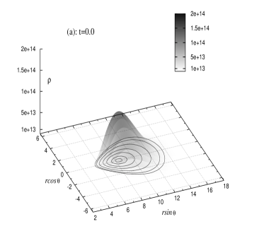
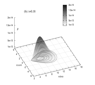
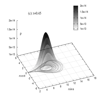
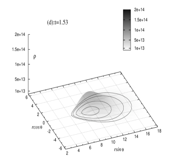
Figure 6: Rest-mass density distributions of a perturbed toroidal neutron star at different times. The sequence illustrates the periodic behaviour during the first cycle of an oscillation excited with $\eta=0.06$. The iso-density contours plotted on the $(r\sin\theta,r\cos\theta)$ planes of the different panels can be used to trace the motion of the matter and are the same for all of the panels (in particular they refer to $\rho=5.0\times 10^{\;12},1.\times 10^{13},2.5\times 10^{13},5.0\times 10^{13},7.5\times 10^{13},1.0\times 10^{14}$, and $1.11\times 10^{14}\ {\rm g/cm^{3}}$, respectively). The times are expressed in terms of the orbital timescale, the spatial coordinates are in terms of the gravitational radius, and the rest-mass density in ${\rm g/cm^{3}}$. See main text for a comment on the sequence.

Once triggered, the behaviour described above will repeat itself with great regularity (cf. the small insets of Figures 4 and  5) and minimal numerical dissipation (which can be appreciated through the very small decay in the amplitude over 100 dynamical timescales) up until the numerical simulation is stopped or the toroidal neutron star has been entirely accreted by the black hole. During these oscillations, the pressure gradients act as a restoring force during the periodic transformation of the excess kinetic energy (transferred with the initial velocity perturbation) into potential gravitational energy and viceversa. As we shall comment on later, this is a first clue about the nature of these pulsations.

It is worth noting that the introduction of a perturbation in the radial velocity will no longer guarantee that the specific angular momentum is conserved during the time evolution. This can be most easily seen if we rewrite the $\phi$-component of the Euler equations in the form [cf. Eq. (24) of Hawley et al. (1984a)]

$$\partial_{t}\ell=\frac{1}{\rho h\Gamma^{2}\sqrt{-g}}\partial_{i}\left[\sqrt{-g}\rho h\Gamma^{2}v_{\phi}v^{i}\right]\ .$$ (16)

For an unperturbed toroidal neutron star, $v^{r}=v^{\theta}=0=\partial_{\phi}$ and the right-hand-side of Eq. (16) is therefore zero, ensuring the conservation of the specific angular momentum. Clearly, this is no longer true when a small negative radial velocity is introduced and although small, this effect further favours the tiny spill of matter through the edge of the torus.

A final comment should be made about initial models consisting of initially stable toroidal neutron stars $(\Delta W<0)$ and that are therefore fully contained in barotropic surfaces smaller than their Roche lobe. Also for these models we have performed a number of simulations investigating their behaviour for different initial perturbations as well as for different initial masses. Overall, the behaviour observed with these initial data is qualitatively similar to the one already discussed for marginally stable tori, i.e. also these models develop the runaway instability or show a quasi-periodic behaviour depending on whether the spacetime evolution is taken into account or not. The most significant difference observed is that smaller rest-mass accretion rates are generally produced for the same initial perturbation. This is simply due to the fact that in stable models a larger potential barrier is present at the cusp and is therefore increasingly more difficult for a fluid element to reach the black hole as a result of the initial perturbation.

Figure 7: Power spectrum of the mass accretion rate for models (a), (b), and (c). The values on the vertical axis have been suitably normalized to match the power in the fundamental mode and arbitrary units have been used.

5.2.1 Fourier analysis

We have so far commented on the “quasi-periodic” behaviour of the hydrodynamical variables in response to the initial perturbation but we have not yet discussed how periodic is “quasi-periodic”. We have therefore calculated the Fourier transforms of the relevant fluid quantities for a number of different models. As a good representative case, we plot in Figure 7 the power spectrum of the rest-mass accretion for models (a), (b) and (c) of Table 1. The Fourier transform has been calculated with data obtained with an $\eta=0.06$ perturbation and computed over a time interval going up to $t/t_{\rm orb}\simeq 100$. Note that larger values of $\eta$ produce correspondingly higher peaks in the power spectra, but the data in Figure 7 has been suitably normalized to match the power in the first peak.

There are two important features of Figure 7 that need to be pointed out. The first one is that all of the three power spectra shown consist of a fundamental frequency $f_{0}$ (228 Hz for the models considered in Figure 7) and a series of overtones (at 456 and 684 Hz, respectively) in a ratio which can be determined to be $1:2:3:\ldots$ and to an accuracy of a few percent. (Note that overtones higher than the second one have also been measured, although with much lower power than the one found in the first three peaks.) Indeed, the presence of at least three peaks can be detected also in the power spectra of basically all of the fluid variables as well as in the overall displacement of the toroidal neutron star during the oscillations. Interestingly, the power spectra of some fluid variables, such as that of the $L_{2}$ norm of the rest-mass density, seem to show peaks with much lower power also at intermediate frequencies, in particular at frequencies which are in a ratio $1:3/2:2:5/2:\ldots$ with respect to the fundamental one. Because the energy of these peaks is very close to the background noise, it is not clear whether these modes correspond to physical modes or are due to numerical errors. The second important feature is that the peaks in the power spectra of the three models in Figure 7 have all the same frequencies, with differences below $0.1\%$. All of these properties are clearly suggesting that the quasi-periodic response observed is the consequence of some fundamental mode of oscillation of toroidal neutron stars and that, as for isolated neutron stars, it is probably independent even of the presence of a central black hole.

Figure 8: Dependence of the fundamental frequency $f_{0}$ on the average density in a sequence of models having the same mass ratio, $M_{\rm{d}}/M=0.1$. The data refers to simulations with initial perturbations of strength $\eta=0.06$.

Insight on the nature of these modes can be gained if one considers that all of the models reported in Figure 7 refer to toroidal neutron stars with fixed spatial dimensions and specific angular momentum, but with varying mass (cf. Table 1). This has basically been obtained by suitably rescaling the polytropic constant in the EOS. Another property shared by these models is that they all have the same initial average sound speed. We recall that for the ideal fluid configurations considered here, the local sound speed can be calculated as $c_{s}=\sqrt{{\gamma(\gamma-1)p}/[{(\gamma-1)\rho+\gamma p}]}$, which is effectively a constant for models with an initial density distribution given by Eq. (5). As a result, it is not surprising that the peaks coincide in all of the models if the oscillations discussed so far should be associated to the p-modes (or acoustic modes) of the toroidal neutron star. However, proving that the periodic oscillations observed in our simulations can be interpreted as $p$-modes and validating that the presence of modes at intermediate frequencies is not a numerical artifact requires a detailed perturbative analysis and is beyond the scope of this paper. Work is now in progress and preliminary results in this direction seem to confirm the hypothesis that these oscillations represent the vibrational modes of relativistic toroidal neutron stars having time-varying pressure gradients as the restoring force (Rezzolla et al. 2002).

Since the peaks in the power spectra seem related to the average sound speed, the dependence of the fundamental frequency on the properties of the toroidal neutron star needs to be investigated along sequences different from the one consider in Figure 7. As an example, we have reported in Figure 8 the fundamental frequency $f_{0}$ as a function of the average rest-mass density inside the torus. The data refer to the evolution of models (e)–(h) in Table 1, that have different dimensions, specific angular momenta and polytropic constants, but all have the the same mass ratio $M_{\rm t}/M$ (cf. Table 1). Figure 8 shows that an evident correlation exists between the fundamental frequency and the logarithm of the average rest-mass density. A fit to the data indicates that this correlation is (cf. straight line in Figure 8)

$$f_{0}=(122.55\log{\langle{\rho}\rangle}-1201.67)~{}{\rm Hz}\ ,$$ (17)

where $\langle{\rho}\rangle$ is expressed in cgs units. This expression is important as it suggests that a systematic study of these oscillations for different initial models of toroidal neutron stars is possible. Furthermore, it represents a first step towards a relativistic disc-seismology analysis for massive and vertically extended tori in General Relativity, in analogy to the one extensively developed for geometrically thin discs (Kato 2001; Perez et al. 1997; Silbergleit et al. 2001; Rodriguez et al. 2002).

5.2.2 Linear and nonlinear regimes

All of the quasi-periodic behaviour discussed so far is the consequence of the finite size perturbations that have been introduced in the initial configuration. Within this approach a linear regime is expected in which the response of the toroidal neutron star is linearly proportional to the perturbation introduced, and a nonlinear regime when this ceases to be true. The strength of the perturbation which marks the transition between the two regimes can be estimated from Figure 9, where we show the averaged maximum rest-mass density normalized to the central one in the toroidal neutron star.

Figure 9: Averaged maximum rest-mass density normalized to the central one in the toroidal neutron star as a function of the perturbation strength. The small inset shows a magnification of the behaviour in the linear regime and the solid line shows a very good linear fit to the data. The data refers to model (a) and has been averaged over 10 orbital timescales.

A rapid look at Figure 9, in fact, reveals the presence of both the linear and nonlinear regimes with the first one being shown magnified in the inset, and where the solid line shows the very good linear fit to the data. The transition between the two regimes seems to occur for $\eta\simeq 0.05$, with the nonlinear regime producing maximum amplitudes that are $\sim 35\%$ larger than the initial one. A careful analysis of the behaviour of the fluid variables shows that for perturbations with strength $\eta\gtrsim 0.05$, some of the kinetic energy which is confined to the lower order modes in the linear regime, tends to be transferred also to higher order modes (As remarked above, while in Figure 7 we have reported only the first three peaks, the power spectra show the presence of higher order overtones, with up to the seventh one being clearly visible). The nonlinear coupling among different modes and the excitation of higher order overtones is often encountered in Nature where it serves to redistribute the excess kinetic energy before the production of shocks. In practice, the nonlinear coupling deprives of energy the fundamental mode (which is the one basically represented in Figure 9) and is therefore responsible for the decay of $\langle\rho_{\rm max}/\rho_{\rm c}\rangle$ for $\eta\gtrsim 0.1$. Interestingly, when analysed in terms of the power spectra, this effect shows a very distinctive behaviour. As the nonlinear mode-mode coupling becomes effective, the amount of power in the fundamental mode becomes increasingly smaller as the strength of the perturbation is increased. At the same time, the conservation of energy transfers power to the overtones, with the first ones reaching amplitudes comparable to the fundamental one and with the high order ones becoming more and more distinct from the background.

Determining the transition to the nonlinear regime is important to set an approximate upper limit on the amplitude of the oscillations and, as we will discuss in the following Section, it is relevant when estimating the emission of gravitational waves. It should also be noted that in the parameter range for $\eta$ in which we have performed our calculations (i.e. $\eta\in[0.001,0.12]$), the peak frequencies in the power spectra have not shown to depend on the values used for $\eta$. This is of course consistent with them being fundamental frequencies (and overtones).

A final comment should be made on the minimum value of the perturbation parameter $\eta$ which is sufficient to produce the quasi-periodic behaviour described in this Section. On the basis of the continuum equations one expects that this minimum value is strictly larger than zero. However, we have performed simulations of marginally stable configurations $(\Delta W=0)$ with $\eta=0$ and observed much of the phenomenology described above even if at rather minute amplitudes and with a larger numerical noise. This result, which has been encountered also in other accurate simulations of relativistic stars (Font et al. 2002), is not entirely surprising and is simply indicating that in the absence of prescribed perturbations, even the small truncation error introduced in the construction of the initial configuration is sufficient to excite the pulsations in these modes of vibration.

6 Gravitational wave emission

Despite our analysis has been restricted to axisymmetry, two simple considerations suggest that strong quasi-periodic gravitational waves should be expected together with the quasi-periodic accretion. The first of these considerations is that these oscillating tori undergo large and rapid variations of their mass quadrupole moment which, we recall, can be calculated as

$$I\equiv\int\rho\left(\frac{3}{2}z^{2}-\frac{1}{2}\right)r^{4}drdz\ ,$$ (18)

where $z\equiv\cos\theta$. It is therefore reasonable to expect that gravitational waves, with a strain proportional to the second time derivative of Eq. (18), should be produced during such oscillations. The second consideration is suggested by expression (18), which shows that a configuration with toroidal topology and in which the rest-mass density has a maximum away from the origin will naturally have a large mass quadrupole simply because of the product $\rho r^{4}$ in the integrand of this equation. This should be contrasted with what happens for stars with spherical topology and which have instead the largest densities at the centre. Both of these arguments justify the intense gravitational radiation and the large signal-to-noise ratio we have calculated using the Newtonian quadrupole approximation. Before discussing this in detail, however, it is useful to remind that since we are not solving the Einstein field equations, we are unable to account for that part of the gravitational radiation that is emitted by the black hole itself as a result of the quasi-periodic mass accretion. For the same reason we cannot estimate the amount of gravitational radiation that will be captured by the black hole and will not reach null infinity. Work is now in progress to calculate also this part of the radiative field using an approach in which the fluid evolution is used as a “source” for a perturbative form of the Einstein equations.

The presence of an azimuthal Killing vector has two important consequences. Firstly, the gravitational waves produced by these axisymmetric oscillating tori will carry away energy but not angular momentum, which is a conserved quantity in this spacetime. This is to be contrasted with the gravitational wave emission from non-axisymmetric perturbations in a massive torus orbiting a black hole, whose strength has been estimated in recent papers (van Putten 2001a, b; Mineshige et al. 2002). Secondly, the gravitational waves produced will have a single polarization state (i.e. the “plus” one in our coordinate system, Kochanek et al. (1990)), so that the transverse traceless gravitational field is completely determined in terms of its only nonzero transverse and traceless (TT) independent components, $h^{TT}_{\theta\theta}=-h^{TT}_{\phi\phi}$ (Zwerger & Müller 1997). Adopting then Newtonian quadrupole approximation, we can calculate the gravitational waveform $h^{TT}(t)$ observed at a distance $R$ from the source in terms of the quadrupole wave amplitude $A_{20}^{\rm E2}$ (see also Zwerger & Müller 1997)

$$h^{TT}(t)=F_{+}\left(\frac{1}{8}\sqrt{\frac{15}{\pi}}\right)\frac{A_{20}^{\rm E2}(t-R)}{R}\ ,$$ (19)

where $F_{+}=F_{+}(R,\theta,\phi)$ is the detector’s beam pattern function and depends on the orientation of the source with respect to the observer. As customary in these calculations, we will assume it to be optimal, i.e. $F_{+}=1$. The wave amplitude $A_{20}^{\rm E2}$ in Eq. (19) is simply the second time derivative of the mass quadrupole moment and can effectively be calculated without taking time derivatives, which are instead replaced by spatial derivatives after exploiting the continuity and the Euler equations (Finn 1989; Blanchet et al. 2001; Rezzolla et al. 1999) to give

$$A_{20}^{\rm E2}\equiv\frac{d^{2}I}{dt^{2}}=k\!\int\!\!\rho\biggl{[}v_{r}v^{r}(3z^{2}\!-\!1)\!+\!v_{\theta}v^{\theta}(2\!-\!3z^{2})\!-\!v_{\phi}v^{\phi}$$

$$\qquad\qquad\qquad-6z\sqrt{(v^{r}v_{r})(v_{\theta}v^{\theta})(1\!-\!z^{2})}\biggl{.}-r\frac{\partial\Phi}{\partial r}(3z^{2}\!-\!1)$$

$$\qquad\qquad\qquad\,+\,3z\frac{\partial\Phi}{\partial\theta}\sqrt{1\!-\!z^{2}}\biggr{]}r^{2}{\rm d}r{\rm d}z\ ,$$ (20)

where $k=16\pi^{3/2}/\sqrt{15}$, and $\Phi$ is the gravitational potential. Since Eq. (6) is intrinsically Newtonian, it brings up two subtle issues when evaluated within a relativistic context. These basically have to do with the definition of the radial coordinate and with the definition of the gravitational potential appearing in Eq. (6). We have here opted for a pragmatical approach and treated $r$ as the Schwarzschild radial coordinate and computed the gravitational potential in terms of the radial metric function as $\Phi=(1-g_{rr})/2$, which is correct to the first Post-Newtonian (PN) order.

To validate the correct implementation of the integral in Eq. (6), we have considered a stationary torus in stable equilibrium, (i.e. $\Delta W_{\rm in}<0$) and without any perturbation besides the one introduced by the truncation error (i.e. $\eta=0$). Under these circumstances, no gravitational radiation can be produced and the terms in the square brackets of Eq. (6) should therefore compose to give zero identically. When computed numerically, we have found that the sum of these terms is effectively very small and of the order $\sim 10^{-2}$. This small residual in the integrand is due to approximations mentioned above (i.e. the use of the Schwarzschild radial coordinate and the first PN approximation to the gravitational potential) and should be interpreted, in practice, as a consequence of the fact that our tori are highly relativistic objects, whose equilibrium is not exactly given by the balancing of the Newtonian terms in the square brackets. Because of this residual, however, the wave amplitude $A_{20}^{\rm E2}$ will not average to zero over an oscillation but will have a net offset. We account for this by removing the overall residual in the evaluation of the wave amplitude (see also Dimmelmeier et al. 2002 for the discussion of an analogous technique).

Figure 10: Time evolution of the second time derivative of the mass quadrupole, computed for model (a). The solid, dotted and dashed lines correspond to $\eta=0.06,0.04,0.02$, respectively. The inset corresponds to the case $\eta=0.06$ and spans 100 orbital timescales.

Figure 10 shows the time evolution of the wave amplitude $A_{20}^{\rm E2}$ computed for model (a) via the expression (6). The different line types refer to $\eta=0.06,0.04$ and $0.02$, respectively. The computed gravitational waveform exhibits the same periodic behaviour discussed in the previous Sections for several fluid variables and shows oscillations that are in phase with the ones observed in the rest-mass density (cf. Figure 5). Furthermore, and as one would expect, the wave amplitude scales with the strength of the initial perturbation. Note that in the case of a simulation with a dynamical spacetime (not shown in Figure 10), the gravitational waveform does not maintain a constant in time amplitude but, as the runaway instability develops, the variations in $A_{20}^{\rm E2}$ become increasingly large, with an exponential growth rate that matches the one observed in the density evolution.

Since the mass quadrupole and its second time derivative are linear in the rest-mass density [cf. Eq. (6)] and the latter exhibits a quasi-periodic behaviour upon perturbations, it is natural to expect the same linear dependence to be present also in terms of the mass ratio $M_{\rm t}/M$. To verify this we have computed $A_{20}^{\rm E2}$ with an initial perturbation $\eta=0.06$ for models (a), (b), and (c) that, we recall, differ only for their mass $M_{\rm t}$. The results of this analysis are reported in Fig. 11 which shows the behaviour of $A_{20}^{\rm E2}$ over one representative period of oscillation and for the four models. As expected, the scaling of the amplitude is linear with $M_{\rm t}/M$ and this is more clearly shown in the inset where the wave amplitude [including the data for model (d)] is fitted linearly with $M_{\rm t}/M$.

Figure 11: Dependence of the wave amplitude $A^{\rm E2}_{\rm 20}$ on the mass of the torus. The solid, dotted and dashed lines correspond to models (a), (b) and (c), respectively. The data refers to an initial perturbation of strength $\eta=0.06$ and the inset shows a linear fit (solid straight line) of the data, including the one for model (d).

Using Eq. (19), it is possible to derive a phenomenological expression for the gravitational waveform that could be expected as a result of the oscillations induced in the toroidal neutron star. Restricting our analysis to the linear regime for which a simpler scaling is possible, we can express the transverse traceless gravitational wave amplitude for a source in the Galaxy in terms of the relevant parameters in our problem

$$h^{TT}\simeq 2.2\times 10^{-21}\left(\frac{\eta}{0.04}\right)\left(\frac{M_{\rm t}}{0.1\ M_{2.5}}\right)\left(\frac{10\;{\rm Kpc}}{R}\right)\ ,$$ (21)

where we have defined $M_{2.5}\equiv M/(2.5\ M_{\odot})$.

Overall, expression (21) shows that, already in the linear regime for the perturbations, a non-negligible gravitational wave amplitude can be produced by an oscillating toroidal neutron star orbiting around a black hole. This amplitude is indeed comparable with the average gravitational wave amplitude computed in the case of core collapse in a supernova explosion (Zwerger & Müller 1997; Dimmelmeier et al.2002) and can become stronger for larger perturbations or masses in the torus.

Of course, the large wave amplitudes suggested by expression (21) are referred to a galactic source and would become three orders of magnitude smaller for a source located at the edge of the Virgo cluster (i.e. at about 20 Mpc). What is important to bear in mind from expression (21) is that oscillating toroidal neutron stars can be sources of gravitational waves as strong or stronger than a core collapse and that could occur with comparable event rates. This notion then serves as a useful normalization for estimating their relevance. It should also be noted, however, that a strong gravitational wave signal is just a necessary condition for the detectability of the gravitational wave emission from toroidal neutron stars and that additional conditions, such as a sufficiently high event rate or a good matching with the sensitivies of the detectors, need to be met. In the following Section we will discuss these issues in more detail and evaluate the detectability of these potential new sources of gravitational waves.

6.1 Detectability

To assess the detectability of toroidal neutron stars as sources of gravitational radiation we have computed the characteristic gravitational wave frequency and amplitude, as well as the corresponding signal-to-noise ratio for the interferometric detectors that will soon be operative. More specifically we have first computed the gravitational waveform in the frequency domain as the Fourier transform of the traceless transverse waveform in the time domain

$${\tilde{h}}(f)\equiv\int_{-\infty}^{\infty}\,e^{2\pi ift}h^{TT}(t)\,dt\ ,$$ (22)

where $h^{TT}(t)$ is calculated according to Eq. (19) and where we have considered the gravitational wave amplitude computed over a fixed spacetime only. (Hereafter we will indicate $h^{TT}(t)$ simply as $h(t)$.). While in principle the integral in Eq. (22) is over an infinite time interval, in practice $h(t)$ is nonzero only over a finite interval $\tau_{\rm life}$. If the initial model chosen for the toroidal neutron star is not a stable one, this time interval is simply set by the timescale over which the runaway instability develops. If, on the other hand, the initial model is stable, the timescale over which a gravitational wave signal is produced can be considerably longer and is basically set by the time over which the star is able to survive, for instance, against non-axisymmetric instabilities. Hereafter, as a representative timescale for our “realistic” toroidal neutron star model (cf. Section 5.1) we will assume $\tau_{\rm life}\simeq 0.2$ s, while longer/shorter timescales will be assumed for models with smaller/larger initial perturbations (cf. Table 2).

Figure 12: Characteristic wave amplitudes for a perturbed toroidal neutron star with $\eta=0.04$. These amplitudes have been computed using the strain noise estimated for LIGO I for a source located at a distance of 10 Kpc and for LIGO II for a source at a distance of 20 Mpc. The numbers can also be effectively compared with the sensitivity curves of VIRGO and EURO that are similar in this frequency range. Different points refer to different mass ratios, with triangles indicating $M_{t}/M=0.25$ and squares $M_{t}/M=0.1$.

Table 2: Characteristic properties for the detection of the gravitational wave signal emitted by a toroidal neutron star. The first two columns show the mass of toroidal neutron star normalized to the black hole one, as well as the strength of the initial perturbation $\eta$. The following nine columns report the characteristic frequency, the characteristic wave strain and the signal-to-noise ratio computed for the three detectors LIGO I, LIGO II and EURO, assuming a galactic distance for a source detected by LIGO I, and an extragalactic distance for a source detected by LIGO II and EURO. The last column reports the characteristic lifetime for the existence of toroidal neutron stars that are unstable to the runaway instability.

$M_{\rm t}/M$	$\eta$	$f_{c}$ (Hz)	$f_{c}$ (Hz)	$f_{c}$ (Hz)	$h_{c}$	$h_{c}$	$h_{c}$	$S/N$	$S/N$	$S/N$	$\tau_{\rm life}$ (s)
		LIGO I	LIGO II	EURO	LIGO I	LIGO II	EURO	LIGO I	LIGO II	EURO
		(10 Kpc)	(20 Mpc)	(20 Mpc)	(10Kpc)	(20 Mpc)	(20 Mpc)	(10 Kpc)	(20 Mpc)	(20 Mpc)
$0.50$	$0.06$	$234$	$230$	$319$	$5.2\times 10^{-20}$	$2.6\times 10^{-23}$	$2.4\times 10^{-23}$	$98.4$	$0.4$	$7.8$	0.08
$0.50$	$0.04$	$227$	$223$	$243$	$4.3\times 10^{-20}$	$2.1\times 10^{-23}$	$2.1\times 10^{-23}$	$84.4$	$0.4$	$6.4$	0.12
$0.50$	$0.02$	$230$	$229$	$238$	$2.7\times 10^{-20}$	$1.3\times 10^{-23}$	$1.3\times 10^{-23}$	$51.8$	$0.2$	$4.0$	0.16
$0.25$	$0.06$	$231$	$228$	$248$	$2.9\times 10^{-20}$	$1.4\times 10^{-23}$	$1.4\times 10^{-23}$	$55.3$	$0.2$	$4.3$	0.12
$0.25$	$0.04$	$227$	$224$	$239$	$2.4\times 10^{-20}$	$1.2\times 10^{-23}$	$1.2\times 10^{-23}$	$47.4$	$0.2$	$3.6$	0.16
$0.25$	$0.02$	$229$	$228$	$234$	$1.4\times 10^{-20}$	$7.2\times 10^{-24}$	$7.2\times 10^{-24}$	$28.2$	$0.1$	$2.1$	0.19
$0.10$	$0.06$	$230$	$226$	$250$	$1.2\times 10^{-20}$	$6.0\times 10^{-24}$	$6.0\times 10^{-24}$	$23.2$	$0.1$	$1.8$	0.14
$0.10$	$0.04$	$229$	$227$	$239$	$1.0\times 10^{-20}$	$5.1\times 10^{-24}$	$5.0\times 10^{-24}$	$19.9$	$0.1$	$1.5$	0.18
$0.10$	$0.02$	$228$	$227$	$234$	$6.1\times 10^{-21}$	$3.0\times 10^{-24}$	$3.0\times 10^{-24}$	$11.9$	$<0.1$	$0.9$	0.20

Given a detector whose response has a power spectral density $S_{h}(f)$, it is then useful to calculate characteristic frequency of the signal (Thorne 1987)

$$f_{c}\equiv\left[\int_{0}^{\infty}\frac{\langle|{\tilde{h}}(f)|^{2}\rangle}{S_{h}(f)}fdf\right]\left[\int_{0}^{\infty}\frac{\langle|{\tilde{h}}(f)|^{2}\rangle}{S_{h}(f)}df\right]^{-1}\ .$$ (23)

where $\langle|{\tilde{h}}(f)|^{2}\rangle$ denotes an average over randomly distributed angles, that we have simply approximated as $\langle|{\tilde{h}}(f)|^{2}\rangle\simeq|{\tilde{h}}(f)|^{2}$. The characteristic frequency provides a representative measure of where, in frequency, most of the signal is concentrated and is therefore relevant when the gravitational wave signal has a rather broad spectrum in frequency, as is the case in a gravitational core collapse. In the case of an oscillating toroidal neutron star, on the other hand, the signal is basically emitted at the fundamental frequency of oscillation (cf. Table 2), increasing the detectability.

Once the characteristic frequency is known, it can be used to determine the characteristic amplitude as

$$h_{c}\equiv\left[3\int_{0}^{\infty}\frac{S_{h}(f_{c})}{S_{h}(f)}\langle|{\tilde{h}}(f)|^{2}\rangle fdf\right]^{1/2}\ .$$ (24)

It worth remarking that when the characteristic frequency fits well in the minima of the sensitivity curves, the weight ${S_{h}(f_{c})}/{S_{h}(f)}$ in the integral of (24) can significantly increase $h_{c}$ when compared to $h^{TT}$. This is indeed what happens for the toroidal neutron stars considered here (cf. Table 2).

A direct comparison of characteristic amplitude with the root-mean-square strain noise of the detector

$$h_{\rm rms}=\sqrt{fS_{h}(f)}\ ,$$ (25)

finally determines the signal-to-noise ratio at the characteristic frequency as

$$\frac{S}{N}=\frac{h_{c}}{h_{\rm rms}(f_{c})}\ .$$ (26)

In Figure 12 we show the characteristic wave amplitude for sources located at a distance of $R=10$ Kpc and $R=20$ Mpc, as computed for two different values of the toroidal neutron star mass. These amplitudes have been computed for the expected strain noise of LIGO I and LIGO II, but the strain curves of VIRGO (that is similar in this frequency range, Damour et al. (2001)) and of EURO (Winkler 2001) have also been reported for comparison. Interestingly, with small initial perturbations $(\eta=0.04)$ and mass ratios $(M_{\rm t}/M=0.1)$, the computed characteristic amplitudes can be above the sensitivity curves of LIGO I for sources within 10 Kpc and above the sensitivity curve of EURO for sources within 20 Mpc. Both results suggest that a toroidal neutron stars oscillating in the Virgo cluster could be detectable by the present and planned interferometric detectors.

Summarized in Table 2 are the basic properties of the gravitational wave signal emitted by a toroidal neutron star. Most notably, we report: the characteristic frequency, the characteristic wave strain and the signal-to-noise ratios as computed for LIGO I, LIGO II and EURO, as well as the timescale over which the signal has been computed. All of these quantities refer to models with different initial perturbations and located at either 10 Kpc (for LIGO I) or 20 Mpc (for LIGO II and EURO).

The values for the signal-to-noise ratios reported in Table 2 are already interesting, but could become larger in at least three different ways. Firstly, and as remarked above, the signal strength computed does not include the exponential growth in the gravitational waveform that would accompany the runaway instability and that would provide an important contribution to the overall characteristic amplitude, as it is the case in binary mergers. As an illustrative example, consider that if the last 10 ms (i.e. roughly the last 5 oscillations) before the disappearence of an unstable torus at 10 Kpc with $M_{\rm t}/M=0.1$ and an initial perturbation with $\eta=0.02$ were taken into account, they would yield a final $S/N\simeq 90$. This is to be contrasted with the corresponding $S/N=11.9$, obtained when the oscillations are considered on a fixed spacetime (cf. Table 2). Secondly, we here have assumed the lifetime of the tori to be limited by the runaway instability to avoid the uncertainties related to the very existence of the instability when the specific angular momentum is not constant. On the other hand, a toroidal neutron star oscillating for a timescale longer than the one assumed in Table 2 will have a proportionally stronger signal even when the exponentially growing phase is neglected. Again, as an example, it is useful to consider that the model yielding $S/N=11.9$ over 0.2 s would produce a $S/N=16.3$ if $\tau_{\rm life}=0.4$ s. Thirdly, an oscillating toroidal neutron star stable to the runaway instability would probably be subject to viscous or magnetic driven non-axisymmetric instabilities on timescales longer than the ones discussed here. Once the non-axisymmetric deformations are fully developed the torus would then have a mass quadrupole with much larger time variations, losing amounts of energy (and angular momentum) in gravitational waves larger than the ones computed here.

The final point to be addressed is the rate at which the emission of gravitational waves from toroidal neutron stars could be detected. Although a realistic estimate of this rate is very difficult since very little is still known about the formation of toroidal neutron stars, it is reasonable to expect that these objects will be produced in a significant fraction of the events leading to core collapse in supernova explosions, binary neutron star mergers and tidal disruption of neutron stars orbiting a black hole. Because in a volume comprising the Virgo cluster all of these sources are among the most promising ones, overall our results indicate that toroidal neutron stars could potentially be new sources of gravitational radiation and certainly suggest a more accurate analysis.

7 Conclusions

We have performed general relativistic hydrodynamics simulations of axisymmetric massive and compact tori orbiting a Schwarzschild black hole with a constant specific angular momentum. These objects have hydrostatic and hydrodynamical properties (i.e. large masses in small volumes with central rest-mass densities reaching almost nuclear matter density) that make them behave effectively as neutron stars, while possessing a toroidal topology. Our attention has been concentrated on two different aspects of the dynamics of these tori.

The first one was focussed on the suggestion that the toroidal neutron stars might be dynamically unstable to the runaway instability only if suitably chosen initial data were prescribed. To investigate this we have used a time-dependent numerical code that integrates the general relativistic hydrodynamics equations on a curved background using HRSC methods. The evolution of the spacetime is an essential feature for the development of the instability and has been modelled through a sequence of stationary Schwarzschild spacetimes differing only in the total mass content, which is computed in terms of the total rest-mass accreted onto the black hole at each instant. The conclusion reached is that, at least for constant specific angular momentum tori whose self-gravity is neglected, the initial Roche lobe overflow is not a necessary condition for the development of the instability, which represents a natural feature of the dynamics of these objects. Very recent numerical work shows that this conclusion does not necessarily hold when the specific angular momentum is not constant (Font & Daigne 2002b).

The second aspect was focussed on the dynamical response of these relativistic tori to the perturbations that are expected to be present after the catastrophic events that lead to their formation. Upon the introduction of suitably parametrized perturbations, the toroidal neutron stars have shown a regular oscillatory behaviour resulting both in a quasi-periodic variation of the mass accretion rate as well as of the rest-mass distribution. This response has been interpreted in terms of the excitation of oscillations modes which could be associated with the $p$-modes of toroidal neutron stars. These modes, which have been detected both in their fundamental frequencies as well as in their overtones, depend systematically on the average density of the tori, and a disco-seismologic analysis could provide important information on the physical properties of these toroidal neutron stars.

High rest-mass densities together with a toroidal topology are the basic properties that yield large mass quadrupoles for these toroidal neutron stars. As a consequence of the excitation of oscillations, the mass quadrupoles are induced to change rapidly and intense gravitational radiation is thus produced. Estimates made within the Newtonian quadrupole approximation have shown that strong gravitational waves can be produced during the short lifetime of these tori. In particular, the gravitational radiation emitted by these source is comparable or larger than the one that is expected during the gravitational collapse of a stellar iron core, with a rate of detectable events which could also be larger given the variety of physical scenarios leading to the formation of a massive torus orbiting a black hole. Overall, the strength of the gravitational waves emitted and their periodicity are such that signal-to-noise ratios $\sim{\cal O}(1)-{\cal O}(10)$ can be reached for sources at 20000 or 10 Kpc respectively, making these new sources of gravitational waves detectable and potentially important.

The results reported here are a first step towards the understanding of the dynamics of toroidal neutron stars and call for a number of natural extensions and improvements. In particular, we plan to extend the simulations to the more realistic scenario of non-constant angular momentum tori, in order to find out if our conclusions regarding both the oscillation properties of toroidal neutron stars and the large amplitude of the associated gravitational wave emission still hold. In addition, it is interesting to improve, using more accurate approaches, the calculation of the gravitational radiation from the oscillations as well as from the runaway instability in the region of the parameter space where the instability could exist (Font & Daigne 2002b). Equally interesting is to include the effects introduced by self-gravity of the torus and determine the quantitative differences that will be encountered in this case. Last but not least, it is worth analyzing how the presence of a Kerr black hole would modify the present results, determining, in particular, the dependence of this phenomenology on the spin of the central black hole.

The results obtained here also provide promising suggestions for further work in a number of research areas different from the ones considered here. Firstly, they indicate that more needs to be investigated about the oscillation properties of relativistic tori and geometrically thick discs. Secondly, they suggest the possibility that the phenomenology observed in the quasi-periodic X-ray luminosity existing in LMXB’s might be related, in some form, to the quasi-periodic accretion resulting from oscillation modes of the discs (Markovic & Lamb 1998; Psaltis & Norman 2000; Wagoner et al. 2002). Thirdly, and perhaps most importantly, these results show that new and unexpected sources of gravitational radiation could exist and might be observed when the new detectors of gravitational radiation become fully operative in the near future.

References

- Abramowicz (1974) Abramowicz M. A., 1974, Acta Astron., 24, 45
- (2) Abramowicz M. A. Jaroszyński M. & Sikora M., 1978, A&A, 63, 221.
- Abramowicz et al. (1983) Abramowicz M. A., Calvani M., Nobili L., 1983, Nature, 302, 597
- Abramowicz et al. (1998) Abramowicz M. A., Karas V., Lanza A., 1998, A&A, 331, 1143
- Ansorg et al. (2002) Ansorg M., Kleinwäcther A., Meinel R., 2002, astro-ph/0208267
- Banyuls et al. (1997) Banyuls F., Font J. A., Ibáñez J. M., Martí J. M., Miralles J. A., 1997, ApJ, 476, 221
- Blanchet et al. (2001) Blanchet L., Damour T., Schäfer G. 1990, MNRAS, 242, 289
- Boyer (1965) Boyer R. H., 1965, Proc. Cambridge Phil. Soc. 61, 527
- Brandt et al. (2000) Brandt S., Font J. A., Ibáñez J. M., Massó J., Seidel E., 2000, Comput. Phys. Comm., 124, 169
- Daigne & Mochkovitch (1997) Daigne F., Mochkovitch R., 1997, MNRAS, 285, L15
- Damour et al. (2001) Damour T., Iyer B. R., Sathyaprakash B. S. 2001, Phys. Rev. D, 63, 044023
- (12) Dimmelmeier H., Font J. A., Müller E., 2002, A&A, 393, 523
- Donat & Marquina (1996) Donat R., Marquina A., 1996, J. Comp. Phys., 125, 42
- Finn (1989) Finn L. S. in Frontiers in Numerical Relativity, ed. C.R. Evans, S. L. Finn., & D.W. Hobill, Cambridge University Press, Cambridge, England, 1989
- Fishbone & Moncrief (1976) Fishbone L. G., Moncrief V., 1976, ApJ, 207, 962
- Font (2000) Font J. A., 2000, Living Reviews in Relativity, 3, 2
- Font et al. (2002) Font J. A., Goodale T., Iyer S., Miller M., Rezzolla L., Seidel E., Stergioulas N., Suen W., Tobias M., 2002, Phys. Rev. D 65, 084024
- Font & Ibáñez (1998a) Font J. A., Ibáñez J. M., 1998a, ApJ, 494, 297
- Font & Daigne (2002a) Font J. A., Daigne F., 2002a, MNRAS, 334, 383
- Font & Daigne (2002b) Font J. A., Daigne F., 2002b, ApJL, submitted
- Hawley et al. (1984a) Hawley J. F., Wilson J. R., Smarr L. L., 1984a, ApJ, 277, 296
- Igumenshchev & Beloborodov (1997) Igumenshchev I. V., Beloborodov A. M., 1997, MNRAS, 284, 767
- Kato (2001) Kato S., 2001, PASJ, 53, 1
- Kochanek et al. (1990) Kochanek C., Shapiro S. L., Teukolsky S. A. Chernoff D. F., 1990, ApJ, 358, 81
- Kozlowski et al. (1978) Kozlowski M., Jaroszynski M., Abramowicz M. A., 1978, A&A, 63, 209
- Lee & Kluzniak (1999a) Lee W. H., Kluzniak W., 1999a, MNRAS, 308, 780
- Lee & Kluzniak (1999b) Lee W. H., Kluzniak W., 1999b, ApJ, 526, 178
- Lee (2000) Lee W. H., MNRAS, 318, 606
- MacFayden & Woosley (1999) MacFayden A. I., Woosley S. E., 1999, ApJ, 524, 262
- Markovic & Lamb (1998) Markovic D., Lamb F. K., 1998, ApJ, 507, 316
- Masuda & Eriguchi (1997) Masuda N., Eriguchi Y., 1997, ApJ, 489, 804
- Masuda et al. (1998) Masuda N., Nishida S., Eriguchi Y., 1998, MNRAS, 297, 1139
- Meszaros (2002) Meszaros P., 2002, ARA&A, 40, 137
- Michel (1972) Michel F., 1972, Astrophys. Spa. Sci., 15, 153
- Mineshige et al. (2002) Mineshige S., Hosokawa T., Machida M., Matsumoto R. 2002, astroph/0208406
- Novikov & Thorne (1973) Novikov I., Thorne K. S., 1973, in Black Holes, eds. B. de Witt and C. de Witt, Gordon and Breach, NY 491, 663
- Perez et al. (1997) Perez C. A., Silbergleit A. S., Wagoner R. V., Lehr D. E., 1997, ApJ, 476, 589
- Psaltis & Norman (2000) Psaltis D., Norman C., astro-ph/0001391
- Rezzolla et al. (1999) Rezzolla L., Shibata M., Asada H., Baumgarte T. W. Shapiro S. L., 1999 ApJ, 525, 935
- Rezzolla et al. (2000) Rezzolla L., Lamb F. K., Shapiro S. L., 2000 ApJL, 531, L141
- Rezzolla et al. (2002) Rezzolla L., Yoshida S’i., Zanotti O., 2002 in preparation
- Rodriguez et al. (2002) Rodriguez M. O., Silbergleit A. S., Wagoner R. V., 2002, ApJ, 567, 1043
- Ruffert & Janka (1999) Ruffert M., Janka H.-T., 1999, A&A, 344, 573
- Ruffert & Janka (2001) Ruffert M., Janka H.-T., 2001, A&A, 380, 544
- Shakura & Sunyaev (1973) Shakura N. I., Sunyaev R. A., 1973, A&A, 24, 337
- Shibata & Uryū (2000) Shibata M., Uryū K., 2000, Phys. Rev. D, 61, 4001
- Shibata (2002) Shibata M., 2002, Talk given at the IV Meeting of the European Network on “Sources of Gravitational waves”, Palma de Mallorca, Spain
- Silbergleit et al. (2001) Silbergleit A. S., Wagoner R. V., Rodriguez M. O., 2001, ApJ, 548, 335
- Spruit (1999) Spruit H. C., 1999, A&A, 341, L1
- Thorne (1987) Thorne K. S. in 300 Years of Gravitation, edited by S. W. Hawking ans W. Israel, Cambridge University Press, Cambridge, England, 1987
- Wagoner et al. (2002) Wagoner R. V., Silbergleit A. S., Rodriguez M. O., 2001, ApJ, 559, L25
- Wilson (1984) Wilson D. B., 1984, Nature, 312, 620
- van der Klis (2000) van der Klis M., 2000, ARA&A, 38, 71
- van Putten (2001a) van Putten M. H. P. M., 2001, Phys. Rev. Lett. 87, 091101
- van Putten (2001b) van Putten M. H. P. M., 2001, ApJ. 575, L71
- Vietri & Stella ( 1998) Vietri M., Stella L. 1998, ApJ. 507, L45
- Winkler ( 2001) Winkler W., for “The VIRGO/GEO Collaboration”, Vision document www.astro.cf.ac.uk/geo/euro/
- Zwerger & Müller (1997) Zwerger T., Müller E., 1997, A&A, 320, 209