Toward Stable 3D Numerical Evolutions of Black-Hole Spacetimes

Abstract

Three dimensional (3D) numerical evolutions of static black holes with excision are presented. These evolutions extend to about $8000M$, where $M$ is the mass of the black hole. This degree of stability is achieved by using growth-rate estimates to guide the fine tuning of the parameters in a multi-parameter family of symmetric hyperbolic representations of the Einstein evolution equations. These evolutions were performed using a fixed gauge in order to separate the intrinsic stability of the evolution equations from the effects of stability-enhancing gauge choices.

Recent studies have documented the fact that constraint-violating instabilities are a common (if not universal) feature of solutions to the Einstein evolution equations Kidder et al. (2001); Laguna and Shoemaker (2002); Lindblom and Scheel (2002). Initial data with small numerical errors on some initial Cauchy surface will typically evolve to a solution in which the constraints grow exponentially with time. Black-hole spacetimes that are evolved in full 3D (without symmetry) with a fixed gauge using one of the “standard” formulations of the evolution equations (e.g. ADMArnowitt et al. (1962); York (1979) or BSSNShibata and Nakamura (1995); Baumgarte and Shapiro (1999)) have instabilities of this type that become unphysical (e.g. because the constraints become large) on a timescale of about 100$M$ Yo et al. (2002); Alcubierre et al. (2000), where $M$ is the mass of the black hole. Several studies have shown that changing the evolution equations by adding multiples of the constraints and by changing the dynamical fields can have a significant effect on the growth rate of these constraint-violating instabilities Kidder et al. (2001); Laguna and Shoemaker (2002); Lindblom and Scheel (2002). Such a re-formulation of the BSSN evolution equations has allowed full 3D evolutions with fixed gauge to persist for about 1400$M$ Shoemaker and Laguna (2002). The duration of black hole evolutions has also been extended considerably, apparently indefinitely in some cases, by imposing symmetries, e.g. octant, on the solutions Alcubierre and Brügmann (2001) or by using an appropriate dynamical gauge Yo et al. (2002); Alcubierre et al. (2002).

We present new results for evolving isolated static black holes using a multi-parameter family of symmetric hyperbolic representations of the Einstein evolution equations Kidder et al. (2001). For the optimal case our evolutions extend to about $8000M$. We focus on the question of how the evolution equations themselves affect stability, and therefore we use a fixed gauge  and do not impose any symmetries on the solutions. The fine tuning needed to achieve optimal stability for evolving a single black hole requires a special choice of the parameters in our representation of the evolution equations, but does not require any fine tuning of our numerical methods. Thus we expect that any numerically stable evolution code that solves this same system of equations with the same initial data and boundary conditions will exhibit the same behavior we find here.

We study the evolution of black-hole spacetimes using a particular 12-parameter family of representations of the Einstein evolution equations Kidder et al. (2001). This family is derived from the standard 3+1 “ADM” form of the equations by introducing five parameters $\{\gamma,\zeta,\eta,\chi,\sigma\}$ that densitize the lapse function and add multiples of the constraints to the evolution equations, and seven additional parameters $\{\hat{z},\hat{k},\hat{a},\hat{b},\hat{c},\hat{d},\hat{e}\}$ that re-define the set of dynamical fields. The details of the resulting evolution equations and the precise definitions of these various parameters are explained at length elsewhere Kidder et al. (2001); Lindblom and Scheel (2002), and will not be repeated here. It has been shown that a 9-parameter subfamily of these representations consists of strongly hyperbolic evolution equations in which all of the characteristic speeds of the system (relative to the hypersurface-normal observers) have only the physical values: $\{0,\pm 1\}$ Kidder et al. (2001). It has also been shown that the evolution equations for an open subset of this 9-parameter family, in particular those representations with $-\frac{5}{3}<\zeta<0$, are symmetric hyperbolic Lindblom and Scheel (2002). Our numerical analysis here is confined to this 9-parameter family of symmetric hyperbolic representations of the Einstein evolution equations having physical characteristic speeds.

Here we analyze the numerical evolution of initial data that represents a single isolated static black hole. For initial data we use a $t={\rm constant}$ slice of the Schwarzschild geometry written in Painlevé-Gullstrand coordinates Martel and Poisson (2001),

$$ds^{2}=-dt^{2}+\left(dr+\sqrt{\frac{2M}{r}}dt\right)^{2}+r^{2}d\Omega^{2},$$ (1)

(where $d\Omega^{2}$ is the standard metric on the unit sphere), plus small perturbations that are added by hand. By explicitly inserting the same perturbations for all numerical resolutions, we are able to test convergence; this would not be the case if instead we allowed the perturbations to arise from machine roundoff error. The exact form of the perturbations is unimportant; it does not affect either the asymptotic growth rate of the unstable mode or its spatial dependence.

We also fix the gauge for these evolutions (not just at the initial time but throughout the evolution) by setting the densitized lapse and the shift to those of Eq. (1). Fixing the gauge in this way is known to be less stable than using a carefully selected dynamically determined gauge Yo et al. (2002); Alcubierre et al. (2000). However, our purpose here is to study the intrinsic stability of the evolution equations, so we choose to fix the gauge in this non-optimal way in order to isolate and emphasize this instability.

The evolution equations are solved here using a pseudospectral collocation method (see Kidder et al. (2001, 2000, ) for further details on the implementation) on a 3D spherical shell extending (typically) from $r=1.9M$ to $r=11.9M$. This code utilizes the method of lines; the time integration is performed using a fourth-order Runge-Kutta algorithm. Although we use spherical coordinates, our fundamental variables are the Cartesian components of the various fields. The inner boundary lies inside the event horizon; at this boundary all the characteristic curves are directed out of the domain (into the black hole), so no boundary condition is required there and none is imposed (“horizon excision”). At the outer boundary we require that all ingoing characteristic fields be time-independent, but we allow all outgoing characteristic fields to propagate freely.

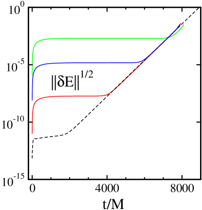
Figure 1: Energy norm $||\delta E||{}^{1/2}$ (per unit volume) for the most stable set of evolution parameters. Solid curves are $||\delta E||{}^{1/2}$ from the full non-linear evolution code, and the dashed curve is from a linearized version of the code.

Recent analytical work Lindblom and Scheel (2002) has shown that the growth rates of the constraint-violating instabilities for the Painlevé-Gullstrand form of the Schwarzschild geometry depend on just three of the nine parameters that specify the evolution equations, $\{\gamma,\zeta,\hat{z}\}$. We confine our study here to the dependence of this instability on the two parameters $\{\gamma,\hat{z}\}$ , and we fix the remaining parameters to the values that define System III of Ref. Kidder et al. (2001).

Figure 2: Solid curve shows the evolution of the integral norm of all the constraints $||{\cal C}_{kij}{\cal C}^{kij}+{\cal C}_{k}{\cal C}^{k}+{\cal C}_{klij}{\cal C}^{klij}+{\cal C}^{2}||^{1/2}$ (per unit volume) for the most stable set of evolution parameters. Dotted curves show the individual contributions from the various constraints: ${\cal C}_{kij}{\cal C}^{kij}$, ${\cal C}_{klij}{\cal C}^{klij}$, ${\cal C}_{k}{\cal C}^{k}$ and ${\cal C}^{2}$, (in that order from largest to smallest at late times).

Figure 1 shows numerical results from the evolution of a single black hole for the case $\gamma=-12$, $\hat{z}=-0.425$. Plotted is the energy norm $||\delta E||{}^{1/2}$ (as introduced in Ref. Lindblom and Scheel (2002)), which measures the deviation of the numerical solution from an exact solution that satisfies the constraints. The solid curves in Figure 1 represent computations performed at different spectral resolutions (18, 24, and 32 radial collocation points), and thus illustrate the convergence of our solutions. The dashed curve represents the evolution obtained with a linearized version of the code, normalized so that the amplitude of the unstable mode is the same as that obtained with the non-linear evolution. The convergence of these solutions, as illustrated in Fig. 1, is made possible by choosing the same initial data, including the exact same form for the initial perturbation added by hand to Eq. (1), for each resolution. If we had instead chosen initial data given by Eq. (1) plus random perturbations (either supplied by numerical roundoff error or introduced by hand) we would not expect results using different resolutions to converge to the same solution.

Figure 2 shows the evolution of the integral norm of the constraints (see Refs. Kidder et al. (2001); Lindblom and Scheel (2002) for definitions of the constraint variables) for the highest-resolution case shown in Figure 1. Note that at late times, most of the constraints in Figure 2 grow at the same rate ($1/\tau\approx 1/275M$) as the energy norm shown in Figure 1. The exception is the Hamiltonian constraint, which is much smaller than the other constraints, but grows at double the growth rate, $1/\tau\approx 1/137M$. Thus it appears that for the optimal choice of parameters, the unstable mode violates the Hamiltonian constraint only to second order in the mode amplitude.

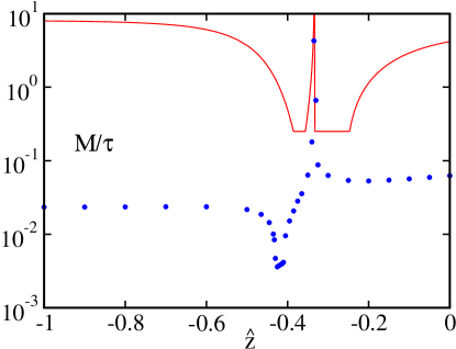
Figure 3: Exponential growth rates of the constraint-violating instabilities as a function of the parameter $\hat{z}$ (with fixed $\gamma=-12$). Points are numerically determined rates, while the solid curve is the approximate growth rate.

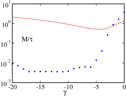
Figure 4: Exponential growth rates of the constraint-violating instabilities as a function of the parameter $\gamma$ (with fixed $\hat{z}=-0.425$). Points are numerically determined rates, while the solid curve is the approximate growth rate.

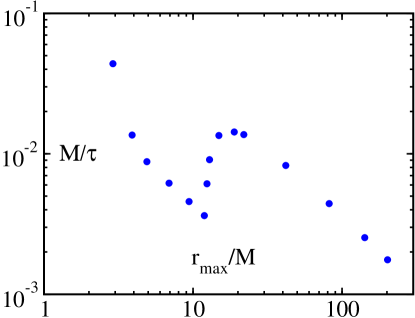
Figure 5: Instability growth rates as a function of the location of the outer boundary of the computational domain for the evolution parameter values $\gamma=-12$, $\hat{z}=-0.425$.

Given a numerical evolution for a particular set of parameters, we determine the exponential growth rate by measuring the slope of the curve in Figs. 1 or 2. Figures 3 and 4 illustrate these growth rates as functions of the parameters $\gamma$ and $\hat{z}$. The points in these figures represent numerically determined growth rates measured using the linearized code (which yields the same growth rates as the fully nonlinear code, see Figure 1 and Ref. Lindblom and Scheel (2002)). The solid curves represent the simple a priori estimates of these growth rates introduced in Ref. Lindblom and Scheel (2002). Although the agreement between the estimates and the numerical results is only approximate, this agreement was good enough to allow us to direct our search for the most stable values of the parameters to the relevant region of the parameter space. The curves in these figures represent orthogonal slices of the function $1/\tau(\gamma,\hat{z})$ through its minimum, $1/\tau_{\max}=1/275M$, which occurs at the parameter values $\gamma=-12$ and $\hat{z}=-0.425$. This minimum growth rate is such that constraint violations in the initial data that are comparable to typical machine precision (e.g. $10^{-16}$) will become large (e.g. of order 0.1) when $t\approx 10^{4}M$. Figures 1 and 2 illustrate the full non-linear evolution that corresponds to this optimal choice of parameters.

For all the cases discussed so far, the outer boundary radius was set at $r_{\rm max}=11.9M$. Figure 5 illustrates the dependence of the growth rate $1/\tau$ on the location of the outer boundary of our computational domain, for fixed $\gamma=-12$ and $\hat{z}=-0.425$. This curve shows a sharp local minimum at the radius where the optimal set of evolution parameters $\{\gamma,\hat{z}\}$ was determined, strongly suggesting that these optimal values depend on the location of this outer boundary. We have verified this by studying in some detail the case where the outer boundary is located at $r_{\rm max}=81.9M$. There we find that the new optimal values of the parameters become $\gamma=-12$ and $\hat{z}=-0.41$, and the value of the growth rate at these new optimal parameters becomes $1/\tau=1/333M$. This growth rate is about 20% smaller than that of the system whose evolution is illustrated in Fig. 1. Thus we infer that the evolution of a single black hole in this case would extend to about $10^{4}M$. We also note that the optimal parameters for $r_{\rm max}=81.9M$ give a value of $1/\tau$ that is about 2/3 the value illustrated in Fig. 5 for this value of $r_{\rm max}$. Considerable additional computational effort will be required to determine the general dependence of the optimal value of $1/\tau$ on $r_{\rm max}$, and we postpone that to a future study. For $r_{\rm max}<12M$ and for $r_{\rm max}>20M$, the growth rate for a fixed set of evolution parameters decreases roughly like $\Lambda/r_{\rm max}$, with the constant $\Lambda$ being about a factor of six larger for the case with $r_{\rm max}>20M$. However, the optimal value of $1/\tau$ as a function of $r_{\rm max}$ does not scale in this simple way. The smallest growth rate determined in our study to date is the point at $\gamma=-12$ and $\hat{z}=-0.425$ with $r_{\rm max}=201.9M$, where we find $1/\tau=1/570M$. This evolution would be expected to persist for over 16,000$M$.

Finally, we note that all of the numerical evolutions discussed so far have placed the inner boundary of the domain at $r_{\rm min}=1.9M$. We have also run the code with $r_{\rm min}=1.0M$ and $r_{\rm min}=1.5M$ for our best-studied case $(\gamma=-12,\hat{z}=-0.425,r_{\rm max}=11.9M)$ and we find that the growth rate is the same to three significant digits.

In summary, we have illustrated that significant improvements in the stability of numerical evolutions of 3D black-hole spacetimes can be achieved by a careful choice of the representation of the Einstein evolution equations. In particular we have shown that single black hole spacetimes can be evolved longer than $t\approx 8000M$ even with fixed gauge. These new results also indicate that the outer boundary conditions may play a significant role in fixing the optimal formulation of the equations, as has been suggested by other investigations Friedrich and Nagy (1999); Calabrese et al. (2001); Szilágyi and Winicour (2002); Calabrese et al. (2002). The role of these boundary conditions will be explored more thoroughly in a future study.