Radiative falloff in the background of rotating black holes

Abstract

We study numerically the late-time tails of linearized fields with any spin $s$ in the background of a spinning black hole. Our code is based on the ingoing Kerr coordinates, which allow us to penetrate through the event horizon. The late time tails are dominated by the mode with the least multipole moment $\ell$ which is consistent with the equatorial symmetry of the initial data and is equal to or greater than the least radiative mode with $s$ and the azimuthal number $m$.

The late time dynamics of black hole perturbations has been studied for over three decades. Complete understanding of the late-time dynamics is available for a Schwarzschild background: Generic perturbation fields of either scalar, electromagnetic, or gravitational fields decay at late times along an $r={\rm const}$ curve as an inverse power of time. Specifically, linearized fields (the scalar field itself, or the Teukolsky function $\psi$ in the gravitational case) decay as $t^{-(2\ell+3)}$ (assuming that the initial data have compact support and are not time-symmetric), where $\ell$ is the multipole moment of the perturbation field price ; barack ; gundlach1 . This behavior was confirmed also for fully nonlinear collapse of spherical scalar fields gundlach2 ; burko-ori . The mechanism which is responsible for this behavior is the scattering of the field off the curvature of spacetime asymptotically far from the black hole.

Because it is only the asymptotically far geometry which determines the behavior of the late-time tails, it is natural to expect similar behavior also when the black hole is rotating poisson . Because spacetime is not spherically symmetric, however, spherical-harmonic modes do not evolve independently. Specifically, taking the initial data of the perturbation field to be a pure $Y^{\ell m}$ mode, other modes are excited. Intuitively, all the modes which are not disallowed [by symmetry requirements (such as the equatorial symmetry of the initial data) or dynamical considerations (such as that only modes with $-\ell\leq m\leq\ell$ are allowed)] will be excited. In particular, modes with $\ell$ values smaller than the original $\ell$ will be excited, and will dominate at late times. (Notice that because the background is axially symmetric, modes with different values of $m$ are not excited when linearized perturbation theory is applied.) Accordingly, the late-time dynamics is dominated by the mode with the least $\ell$ which is excited, namely the smallest $\ell$ which is not disallowed. That is, all modes $\ell$ which are not smaller than $|m|$ and $|s|$, where $s$ is the spin weight of the field, and which respect the equatorial symmetry of the initial data, will be excited. The falloff rate is then $t^{-(2\ell_{\rm min}+3)}$, where $\ell_{\rm min}$ is the smallest mode which can be excited.

Despite the simplicity of this intuitive picture, recent papers report conflicting results. An analytical analysis by Hod — in which the author attempted to find the asymptotic behavior of the fields in the spacetime of a Kerr black hole — yielded results which are more complicated: The decay rate for a scalar field is predicted by Hod to be hod-scalar $t^{-(2\ell^{*}+3)}$ if $\ell^{*}=m$ or $\ell^{*}=m+1$, $t^{-(\ell^{*}+m+1)}$ if $\ell^{*}-m\geq 2$ is even, and $t^{-(\ell^{*}+m+2)}$ if $\ell^{*}-m\geq 2$ is odd, where $\ell^{*}$ is the initial value of $\ell$. For gravitational perturbations Hod’s formula is hod-prl $t^{-(\ell^{*}+\ell_{0}+3-q)}$ (for axisymmetric perturbations), where $\ell_{0}$ is the radiative mode with the least value of $\ell$, and $q={\rm min}(\ell^{*}-\ell_{0},2)$. [Different, apparently conflicting results were reported by Barack and Ori barack-ori . Those authors assumed that the mode $\ell,m=0$ is present in the initial data (for $s=0$), as a result of which it is not straightforward to confront their predictions with Hod’s.]

Although Hod’s results could be relevant for an intermediate regime for carefully chosen parameters, they make only little sense for describing the intended asymptotic late-time behavior. These eerie conclusions imply that some sort of a “memory effect” takes place: the field somehow “remembers” its initial configuration, despite being a linearized field. We do not believe that such a “memory effect” is reasonable: Take the initial data at the time $t_{0}$ to be those of the pure mode $\ell^{*}$, such that $\ell^{*}$ is significantly larger than $\ell_{\rm min}$. At the time $t_{1}>t_{0}$ the field includes, in addition to the mode $\ell^{*}$, also contributions from modes $\ell<\ell^{*}$ because of the excitation of other $\ell$ modes. Now the fields at $t=t_{1}$ can be construed as the initial data of a new evolutionary problem. In the new problem the initial data are a mixture of modes, such that modes $\ell$ smaller than $\ell^{*}$ are present poisson . Because the mode with the smallest existing $\ell$ value dominates at late times and determines the decay rate of the tail, we can see no way in which the $\ell^{*}$ mode can determine the asymptotic late-time tail, unless $\ell^{*}$ determines which modes can and which modes cannot be excited. As in the spacetime of a Kerr black hole it is hard to see how a scenario in which modes which are not disallowed can still be excluded, we conclude that “memory effects” are not to be expected. Hod’s results, if correct, suggest to us that an hitherto unsuspected mechanism of selection rules inhibits the excitation of otherwise allowed modes. Such a counter-intuitive theoretical reasoning must have strong numerical support in order not to be discarded.

Conclusions which apparently are similar to Hod’s were obtained more recently by Poisson poisson , who analyzed the scalar-field tails in a general weakly-curved, stationary, asymptotically flat spacetime. We emphasize that unlike Hod’s analysis — which is an attempt to find the asymptotic late-time behavior in the spacetime of a spinning black hole — Poisson’s analysis aims at finding the behavior in a spacetime in which curvature is weak everywhere. While Poisson’s analysis and results are correct for the spacetime he studies, one should use caution when infering from Poisson’s results on the asymptotic late-time behavior in a Kerr geometry: Although the asymptotically-far geometries are similar, the near-field geometries are very different. As we discuss below, that is a crucial element in understanding the late-time behavior.

Hod’s surprising predictions agree with some reported numerical simulations. In particular, for the case $s=0$, $\ell^{*}=0,m=0$ Hod’s formula predicts a decay rate of $t^{-3}$, which is indeed found KLP96 . For the case $s=0$, $\ell^{*}=4,m=0$, however, Hod’s formula predicts a decay rate of $t^{-5}$, whereas the intuitive picture predicts a decay rate of $t^{-3}$. This case was simulated numerically by Krivan krivan , who found a decay rate with a non-intergal index close to $-5.5$. Like Hod, Krivan too tried to find the asymptotic late-time behavior in the Kerr spacetime. Some view this as a loose confirmation of Hod’s prediction poisson , with numerical accuracy of $10\%$, and as an invalidation of the intuitive picture.

In this Rapid Communication we present results from independent numerical simulations for linearized perturbation fields over a Kerr background. Our simulations show a clear falloff rate of $t^{-3}$ for the initial data of $s=0$, $\ell^{*}=4$, $m=0$. The quality of our results invalidates Hod’s prediction for the asymptotic decay rate, and points at difficulties with Krivan’s simulations or their interpretation. In all the cases we have checked, for either a scalar or a gravitational field, we find that the intuitive picture is correct: the late time behavior is dominated by the mode with the lowest value of $\ell$ which can be excited. In particular, no spooky memory effects occur.

We used the penetrating Teukolsky code (PTC) ptc , which solves the Teukolsky equation for linearized perturbations over a Kerr background in the ingoing Kerr coordinates $({\tilde{t}},r,\theta,{\tilde{\varphi}})$. The Kerr metric is given by

$$\,ds^{2}=\left(1-\frac{2Mr}{\Sigma}\right)\,d{\tilde{t}}^{2}-\left(1+\frac{2Mr}{\Sigma}\right)\,dr^{2}-\Sigma\,d\theta^{2}$$

$$-\sin^{2}\theta\left(r^{2}+a^{2}+\frac{2Ma^{2}r}{\Sigma}\sin^{2}\theta\right)\,d{\tilde{\varphi}}^{2}-\frac{4Mr}{\Sigma}\,d{\tilde{t}}\,dr$$

$$+\frac{4Mra}{\Sigma}\sin^{2}\theta\,d{\tilde{t}}\,d{\tilde{\varphi}}+2a\sin^{2}\theta\left(1+\frac{2Mr}{\Sigma}\right)\,dr\,d{\tilde{\varphi}}\,,$$ (1)

where $\Sigma=r^{2}+a^{2}\cos^{2}\theta$, and $M,a$ are the mass and the specific angular momentum, respectively. These coordinates are related to the Boyer-Lindquist coordinates $(t,r,\theta,\varphi)$ through ${\tilde{\varphi}}=\varphi+\int a\Delta^{-1}\,dr$ and ${\tilde{t}}=t-r+r_{*}$, where $\Delta=r^{2}+a^{2}-2Mr$ and $r_{*}=\int(r^{2}+a^{2})\Delta^{-1}\,dr$. Notice that ${\tilde{t}}$ is linear in $t$, so that along $r={\rm const}$, $\partial/\,\partial{\tilde{t}}=\partial/\,\partial t$.

The Teukolsky equation for the function $\psi$ in the ingoing Kerr coordinates can be obtained by implementing black hole perturbation theory (with a minor rescaling of the Kinnersley tetrad ptc ). It is given by

$$(\Sigma+2Mr){{\partial^{2}\psi}\over{\partial\tilde{t}^{2}}}-\Delta{{\partial^{2}\psi}\over{\partial r^{2}}}+2(s-1)(r-M){{\partial\psi}\over{\partial r}}$$

$$-{{1}\over{\sin\theta}}{{\partial}\over{\partial\theta}}\left(\sin\theta{{\partial\psi}\over{\partial\theta}}\right)-{{1}\over{\sin^{2}\theta}}{{\partial^{2}\psi}\over{\partial\tilde{\varphi}^{2}}}-4Mr{{\partial^{2}\psi}\over{\partial\tilde{t}\partial r}}$$

$$-2a{{\partial^{2}\psi}\over{\partial r\partial\tilde{\varphi}}}-i{2s\cot\theta\over\sin\theta}{{\partial\psi}\over{\partial\tilde{\varphi}}}+(s^{2}\cot^{2}\theta+s)\psi$$

$$+2\left[{sr+ias\cos\theta+(s-1)M}\right]{{\partial\psi}\over{\partial\tilde{t}}}=0\,.$$ (2)

Equation (Radiative falloff in the background of rotating black holes) has no singularities at the event horizon, and therefore is capable of evolving data across it. The PTC implements the numerical integration of Eq. (Radiative falloff in the background of rotating black holes) by decomposing it into azimuthal angular modes and evolving each such mode using a reduced 2+1 dimensional linear partial differential equation. The results obtained from this code are independent of the choice of boundary conditions, because the inner boundary is typically placed inside the horizon, whereas the outer boundary is placed far enough that it has no effect on the evolution.

The PTC has been tested in various different situations. First, it yields the correct complex frequencies for the quasi-normal modes of a Kerr black hole for a wide range of values of $a/M$. Second, it has also been shown to yield equivalent results in the context of the close limit collision of two equal mass, non-spinning, non-boosted black holes (to ones obtained from the Zerilli formalism) gaurav . It is stable, and exhibits second-order convergence.

We next set $a/M=0.9$, $s=0$, and $\ell^{*}=4$, $m=0$. The initial gaussian perturbation is taken to be a mixture of ingoing and outgoing waves, and centered about $r=20M$ with a width of $4M$. As discussed above, our expectations are that all the even $\ell$ modes are excited (respecting the equatorial symmetry of the initial data). The least $\ell$ mode which is excited is the $\ell=0$ mode, so that the decay rate we expect is $t^{-3}$. In contrast, the prediction of Hod is for a decay rate of $t^{-5}$. Figure 1 shows the Teukolsky function $\psi$ for these initial data for $\theta=\pi/2$ (the equatorial plane) for three different resolutions. The data clearly indicate stability and second-order convergence.

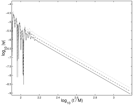
Figure 1: The Teukolsky function $\psi$ as a function of ${\tilde{t}}$ for three different grid resolutions, for $s=0$, $a/M=0.9$, $\ell^{*}=4$, and $m=0$. Dotted line: 8000 steps in $r$ and $40$ steps in $\theta$. Dashed line: 10000 steps in $r$ and $50$ steps in $\theta$. Solid line: 12000 steps in $r$ and $60$ steps in $\theta$. The time step is always taken to be half the step in $r$. The data are shown along $r=20M$ on the equatorial plane.

A decay rate of about $t^{-3}$ is already clear from Fig. 1. Evaluating the decay rate from the slope of the field is very inaccurate: The slope then depends on the interval one chooses, and also on the presence of subdominant modes. The first difficulty can be handled by considering the local power index $n$ burko-ori , which we define as $n\equiv-({\tilde{t}}/\psi)\,\partial_{\tilde{t}}\psi$. The second difficulty can be handled by extrapolating $n$ to timelike infinity. Figure 2A shows $n$ as a function of $M/{\tilde{t}}$. Timelike infinity is at zero, and both the regime where the field is dominated by the quasi-normal ringing and the regime where the field is dominated by the power-law tails are shown. The local power index $n=2.9846$ at ${\tilde{t}}=1500M$. Figure 2B shows the behavior of $3-n$ as a function of $M/{\tilde{t}}$. Clearly, $n$ gets closer with time to the expected value of $3$. In fact, extrapolating $n$ to ${\tilde{t}}\to\infty$ using Richardson’s deferred approach to the limit, we find the asymptotic value of $n$ to be $n_{\infty}=3.0003\pm 0.0011$. Our results suggest that the late-time field is dominated by the $\ell=0$ mode. We checked this by plotting $\psi$ as a function of $\theta$ in Fig. 3 for different values of ${\tilde{t}}$. We indeed find that $\psi$ quickly loses any dependence on $\theta$, such that at late times it is indeed described by the $\ell=0$ mode. Any dependence of $\psi$ on $\theta$ is smaller than 3 parts in $10^{6}$ at ${\tilde{t}}=1000M$.

lpi1.eps

Figure 2: The local power index for the same data as in Fig. 1. Upper panel (A): $n$ as a function of $M/{\tilde{t}}$. Lower panel (B): $\log_{10}|3-n|$ as a function of $M/{\tilde{t}}$. The data are shown for an equatorial curve at $r=20M$.

theta_new.eps

Figure 3: The normalized Teukolsky function $\psi/\psi(\theta=0)$ as a function of $\theta$ at $r=25M$, for the same data as in Fig. 1, for various values of ${\tilde{t}}$. Upper panel: At ${\tilde{t}}=150M$ (dotted line), $200M$ (dash-dotted), $250M$ (dashed), and $300M$ (solid line). Lower panel: At ${\tilde{t}}=400M$ ($\square$), $500M$ ($\ast$), $600M$ ($\circ$), $700M$ (+), $800M$ (dotted line), $900M$ (dash-dotted), $1000M$ (dashed), and $1500M$ (solid line).

Next, we present results for the behavior of fields with higher spins. We set the parameters to $s=2$, $a/M=0.3$, and initial $l^{*}=6$, $m=0$. The pulse is again centered about $r=20M$ with a width of $4M$. The prediction of Hod’s formula for this case is a decay rate of $t^{-9}$. In this case our expectations are that the least $\ell$ mode to be excited is the $\ell=2$ mode. Consequently, we expect the decay rate to be $t^{-7}$. This is indeed confirmed in Fig. 4A, which shows the local power index $n$ as a function of ${\tilde{t}}/M$, and in Fig. 4B which displays $7-n$ as a function of $M/{\tilde{t}}$. At ${\tilde{t}}=1500M$, we find that $n=6.8646$. Extrapolating $n$ to timelike infinity, we find that $n_{\infty}=7.01\pm 0.03$, in agreement with our expectations.

s21.eps

Figure 4: The local power index for $s=2$, $a/M=0.3$, $l^{*}=6$, and $m=0$. Upper panel (A): $n$ as a function of ${\tilde{t}}/M$. Lower panel (B): $\log_{10}(7-n)$ as a function of $M/{\tilde{t}}$. The data are taken for an equatorial curve at $r=20M$.

Our results clearly show that starting with a pure mode $\ell^{*},m$, the late-time decay rate is dominated by the least mode $\ell_{\rm min}$ which is consistent with the equatorial symmetry of the initial data and is equal to or greater than the least radiative mode $\ell_{0}={\rm max}(|s|,|m|)$. The late-time decay rate is given by $t^{-(2\ell_{\rm min}+3)}$. Our conclusions are in sharp disagreement with the recent predictions by Hod hod-prl ; hod-scalar . Hod’s analysis is in the frequency domain, and carried to leading order in $\omega$, the angular frequency. That approach is very successful in the background of a Schwarzschild black hole, where it reproduces the known results andersson . The understanding that the power-law tails result from scattering of the field at asymptotically large distances implies that it is only the small $\omega$ which are responsible for the tails. That is indeed the case with a Schwarzschild black hole. We conjecture that it would also be the case for a Kerr black hole, if there were no excitations of dominating modes which are not present in the initial data. For example, in the case of a scalar field with $\ell^{*}=m=0$, the dominating mode is already present in the initial data. Considering only the small $\omega$ contributions indeed produces a result in agreement with numerical simulations. When the dominating mode is not present in the initial data, however, it needs first to be excited. If it is excited (with any nonzero amplitude), the small $\omega$ approximation may produce the correct result for the decay rate. However, mode-excitation is an effect which is nonlinear in the gravitational potentials, and is strongest in the near zone. This suggests to us that a leading order (in $\omega$) analysis will not, in general, get all the excited modes right. It might be the case that higher orders in $\omega$ are necessary in order to get all the modes which are excited. Our numerical results indeed show, that when the least mode which can be excited $\ell_{\rm min}$ is “far” from the initial $\ell^{*}$, that technique does not produce the former: For example, for initial $\ell^{*}=4$ and $m=0$, the leading order in $\omega$ analysis was able to get the $\ell=1$ mode excited (as is manifested by Hod’s decay rate of $t^{-5}$), but not the $\ell=\ell_{\rm min}=0$ mode (which implies a decay rate of $t^{-3}$). We suggest, that although a frequency-domain analysis is capable of getting the decay rate right, it should include an expansion to higher orders in $\omega$. Such an expansion would be a formidable endeavor. In a similar way, by taking spacetime to be weakly curved everywhere, Poisson tacitly assumed that it is just the far-zone part of the field which is important. (In Poisson’s case, we emphasize, this assumption is well justified, because in the spacetime studied by Poisson spacetime is nowhere strongly curved. Incidentally, Poisson suggests a selection-rule mechanism in the spacetime he studied, which is related to the remarkable vanishing of terms in the initial data in the transformation from spheroidal to spherical coordinates. The mechanism suggested by Poisson demonstrates how indeed Hod’s results could be correct in that context. However, no such mechanism is offered for a Kerr spacetime.) That assumption is equivalent to taking the large-$r$ approximation, or the small-$\omega$ approximation. Consequently, Poisson and Hod make, in fact, the same kind of approximation, such that it is not surprising that they obtain the same results. We emphasize, that Poisson acknowledges that effects which are nonlinear in the gravitational potentials may produce modes with $\ell$ values which are smaller than those obtained by him. Poisson then remarks, that no such effects have been reported on in the literature. Evidence for such an effect is precisely what we find here. Although the late-time expansion method barack-ori does not seem to suffer from similar weaknesses, it is hard to apply for the problem of interest. Starting with an initial $\ell^{*}$ which is “far” from the least mode $\ell_{\rm min}$ to be excited, the method of Ref. barack-ori requires many iterations in order to find the excited mode $\ell_{\rm min}$. Specifically, three iterations are required in order to find the $\ell=0$ mode starting with $\ell^{*}=4,m=0$. Carrying this iterative scheme in practice seems like a daunting task. We would like to repeat, that while Hod’s method fails to obtain the correct asymptotic decay rate, it may still be useful in determining an intermediate behavior for carefully chosen parameters.

Lastly, our results are in disagreement also with the numerical results of Krivan krivan , who reported on a fractional power-law index which is about $-5.5$ for the case of initial $s=0$, $\ell^{*}=4$ and $m=0$. While we cannot point with certainty to the reason why Krivan’s simulations produce a result for the asymptotic late-time behavior which is at odds with ours, we would like to mention some of the factors which may be responsible: Krivan takes the black hole to spin exceedingly fast. In fact, Krivan takes $a/M=0.9999$. The high spin of the black hole may act in two ways: First, it slows down the decay rate of the quasi-normal ringing, such that longer integration times are required in order to obtain the tails. Second, the numerical solution of the Teukolsky equation is more sensitive and harder when the spin is very high. Another factor is related to the location and the direction of Krivan’s initial perturbation. Krivan takes the perturbation to be centered around $r_{*}/M=100$, and to have a very large width (of $100M$). Also, the perturbation is purely outgoing on the initial slice. We thus conjecture that the dominating $\ell=0$ mode is excited only with a very low amplitude, because most of the perturbation field does not probe the strong-field region. This, in addition to the great distance and width of the initial perturbation, may combine into late-time tails whose asymptotic behavior becomes evident only at very late times, to which Krivan’s simulations have not arrived.

The picture which arises for linearized perturbations in the background of a spinning black hole is simpler than that which is implied by. However, we expect the picture to be even simpler than that for fully nonlinear perturbations: When the initial perturbation is not axially symmetric, the evolving spacetime will not be axially symmetric either. Consequently, the $m$ value of the field will not be conserved, and different values of $m$ will also be excited, preserving only the equatorial symmetry of the initial data. We therefore expect a fully nonlinear evolution to yield results which are simpler than those obtained from a linearized analysis: Because $m$ is no longer fixed, the restriction of $\ell_{0}$ is no longer so strict: $\ell_{0}=|s|$, and the dominating mode is simply the least $\ell$ mode which is consistent with the equatorial symmetry which is equal to or greater than $\ell_{0}$. We thus expect generic tails to always have a decay rate of $t^{-(2|s|+3)}$. The more complicated results of this Rapid Communication then are an artifact of the linearization: the full theory is simpler.

We thank Eric Poisson and Richard Price for discussions. This research was supported by NSF grants PHY-9734871 and PHY-0140236. Initial work on this research was done while LMB was at the California Institute of Technology, where it was supported by NSF grant PHY-0099568. We thank the Center for Gravitational Physics and Geometry at Penn State for computational facilities.

References

- (1) R.H. Price, Phys. Rev. D 5, 2419 (1972)
- (2) C. Gundlach, R.H. Price, and J. Pullin, Phys. Rev. D 49, 883 (1994).
- (3) L. Barack, Phys. Rev. D 59, 044017 (1999).
- (4) C. Gundlach, R.H. Price, and J. Pullin, Phys. Rev. D 49, 890 (1994).
- (5) L.M. Burko and A. Ori, Phys. Rev. D 56, 7820 (1997).
- (6) E. Poisson, Phys. Rev. D 66, 044008 (2002).
- (7) S. Hod, Phys. Rev. D 61, 024033 (2000); 61 064018 (2000).
- (8) S. Hod, Phys. Rev. Lett. 84, 10 (2000).
- (9) L. Barack and A. Ori, Phys. Rev. Lett. 82, 4388 (1999).
- (10) W. Krivan et al, Phys. Rev. D 54, 4728 (1996).
- (11) W. Krivan, Phys. Rev. D 60, 101501 (1999).
- (12) M. Campanelli et al, Class. Quantum Grav. 18, 1543 (2001).
- (13) G. Khanna, Phys. Rev. D 65, 124018 (2002).
- (14) N. Andersson, Phys. Rev. D 55, 468 (1997).