LISA, binary stars, and the mass of the graviton

Abstract

We extend and improve earlier estimates of the ability of the proposed LISA (Laser Interferometer Space Antenna) gravitational wave detector to place upper bounds on the graviton mass, $m_{g}$, by comparing the arrival times of gravitational and electromagnetic signals from binary star systems. We show that the best possible limit on $m_{g}$ obtainable this way is $\sim 50$ times better than the current limit set by Solar System measurements. Among currently known, well-understood binaries, 4U1820-30 is the best for this purpose; LISA observations of 4U1820-30 should yield a limit $\approx 3-4$ times better than the present Solar System bound. AM CVn-type binaries offer the prospect of improving the limit by a factor of $10$, if such systems can be better understood by the time of the LISA mission. We briefly discuss the likelihood that radio and optical searches during the next decade will yield binaries that more closely approach the best possible case.

Recent work by Will Will and Larson and Hiscock LH has examined how gravitational wave observations by LIGO LIGO and LISA LISA can be used to place upper bounds on the mass of the graviton. Will’s proposed method utilizes the dispersion of the waves generated in binary inspiral caused by a nonzero graviton mass, while Larson and Hiscock have proposed direct correlation of gravitational wave (GW) and electromagnetic (EM) observations of nearby white dwarf binary star systems. Both approaches promise improved bounds compared to the present bound based on Solar System dynamics, $m_{g}^{SS}<4.4\times 10^{-22}$ eV, which corresponds to a bound on the graviton Compton wavelength of $\lambda_{g}^{SS}=h/m_{g}=2.8\times 10^{12}$ km Talmadge .

The ultimate limit on the binary star method is determined by the precision with which the phase of the gravitational wave signal can be measured. Larson and Hiscock LH estimated this uncertainty in phase by considering the cadence of measurements made by LISA during a one-year integration of the periodic signal from the binary star system. However, this is not the dominant source of uncertainty in the gravitational wave phase measurement. Let $\phi$ be the orbital phase of the binary at some fiducial time. For GW measurements with signal-to-noise $S/N>>1$, one can estimate the uncertainty with which this phase can be extracted by $\delta\phi_{GW}=\sqrt{(\Gamma^{-1})^{\phi\phi}}\bigl{(}1+{\cal O}(S/N)^{-1}\bigr{)}$, where $\Gamma_{ij}$ is the Fisher information matrix. For a circular binary, the signal is characterized by seven or eight physical parameters: two angles describing the direction $\hat{N}$ to the binary (i.e., its position on the sky), two more angles describing the normal $\hat{L}$ to the orbital plane, the overall amplitude $A$, the overall phase $\phi$, the orbital frequency $f_{0}$, and (non-negligible for for some binaries) the frequency derivative $\dot{f}_{0}$. If all parameters except $\phi$ are somehow already known (e.g. if the binary is resolved optically, for example by the Space Interferometry Mission (SIM) SIM ), then $(\Gamma^{-1})^{\phi\phi}=(\Gamma_{\phi\phi})^{-1}=\frac{1}{4}(S/N)^{-2}$ Cutler , so we would estimate $\delta\phi_{GW}\approx\frac{1}{2}\left({S\over N}\right)^{-1}$. More generally we can write

$$\delta\phi_{GW}=\frac{\alpha}{2}\left({S\over N}\right)^{-1}\left(1+{\cal O}(S/N)^{-1}\right)\;\;\;.$$ (1)

where $\alpha(>1)$ is a correction term that accounts for the fact there will generally be additional unknown parameters to be extracted from the GW data, which can only increase $(\Gamma^{-1})^{\phi\phi}$. The case of interest, for setting a limit on $m_{g}$, is where $\delta\phi_{GW}<<1$, or ${S\over N}>>1$, so from now on we ignore the ${\cal O}(S/N)^{-1}$ correction in Eq. (1).

How large is $\alpha$ likely to be? To answer this question, we must consider more carefully the definition of $\phi$, and also consider what information will be available to supplement the GW measurement.

By $\phi$, we will mean the orbital phase, at some fiducial time $t_{0}$, measured from the point in the orbit where the orbital plane intersects the plane perpendicular to the line-of-sight. More precisely,

$$\phi\equiv{\rm tan}^{-1}\bigl{[}(\hat{r}(t_{0})\cdot\hat{y})/(\hat{r}(t_{0})\cdot\hat{x})\bigr{]}$$ (2)

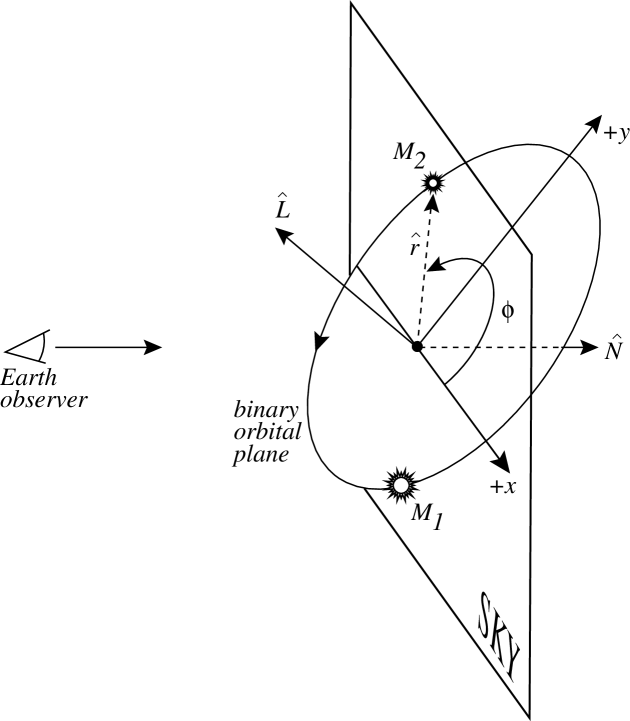
Figure 1: The coordinate system used to define the orbital phase is determined by the line of sight to the binary $\hat{N}$ and the binary orbital angular momentum $\hat{L}$, such that $\hat{x}$ points along the line of nodes, and $\hat{y}$ lies in the orbital plane. The position vector $\hat{r}$ points along the binary axis, from the primary (largest mass , $M_{1}$) to the secondary (smallest mass, $M_{2}$) in the system. The orbital phase $\phi$ is defined to be the angle in the orbital plane between the $+x$ axis and the position vector.

where $\hat{r}$ is the (unit) orbital separation vector (pointing from the more massive to the less massive body), $\hat{x}\equiv\hat{N}\times\hat{L}/||\hat{N}\times\hat{L}||$, and $\hat{y}\equiv\hat{L}\times\hat{x}$. Fig. 1 illustrates these quantities. This is a useful definition when comparing to most EM measurements, where generally one does not know the overall orientation of the binary, but can measure the phase of one body’s motion towards or away from the observer (e.g., by Doppler measurements, or, as discussed below with 4U1820-30, because the flux is greatest at the instant the the body is furthest from the observer). Rather than report the phase at some fiducial time, astronomers typically report some “epoch” (i.e., instant of time) $t_{0}$ when the orbital phase (measured optically) is $\phi_{EM}=0$. Of course, this optical (or X-ray, etc.) measurement will have some error; we define $-\delta\phi_{EM}$ ($\approx-2\pi f_{0}\delta t_{0}$) to be the true EM phase at time $t_{0}$. Our proposal for constraining $m_{g}$ amounts to using LISA to measure $\phi_{GW}(t_{0})$. If photons and gravitons travel at the same speed, then $\phi_{GW}(t_{0})$ should be consistent with zero. More precisely, one can set the following lower bound on the Compton wavelength $\lambda_{g}$ of the graviton (see LH for details):

$$\lambda_{g}=\frac{1}{2f_{0}}\sqrt{\frac{1}{2}\left(1+\frac{2\pi f_{o}D}{\Delta}\right)}\;\;\;,$$ (3)

where $D$ is the distance to the binary system and $\Delta$ is defined by 

$$\Delta=\sqrt{\delta\phi_{EM}^{2}+\delta\phi_{GW}^{2}}\;\;\;.$$ (4)

Note that in Eq. (4) we have assumed that the errors $\delta\phi_{EM}$ and $\delta\phi_{GW}$ are uncorrelated.

Eq. (2) represents one convention for the zero-point of the phase $\phi$; with a different convention, Eqs. (3)–(4) would remain valid, but with different numerical values for $\delta\phi_{EM}$ and $\delta\phi_{GW}$. Obviously, for any given binary, one wants to define $\phi$ in a way that minimizes $\Delta$. For instance, if the binary is seen nearly face-on (i.e., $\hat{L}$ and $\hat{N}$ are nearly parallel), then the $\phi$ defined in Eq. (4) is difficult to measure, since a small shift in $\hat{L}$ can produce a large shift in $\phi$, for fixed $\hat{r}(t_{0})$. In this case, if one could somehow resolve the two components of the binary optically (e.g., with SIM), then one would probably be better off choosing some arbitrary-but-easily-determined direction (e.g., the direction to Polaris) to define $\phi=0$.

For the purpose of determining the best possible upper limit one can set on $\lambda_{g}$, we will next assume that $|\delta\phi_{EM}|$ is small compared to $|\delta\phi_{GW}|$. We expect this will generally be the case when one can determine the optical phase at all (because of the much higher $S/N$ one typically has with optical measurements), but this will have to be verified on a case-by-case basis. Combining Eqs. (1), (3), and (4) with this assumption then allows us to obtain a simple expression for the best possible limit achievable on the Compton wavelength of the graviton from combined EM and GW observations of binary systems:

$$\lambda_{g}\simeq{\pi\over{\sqrt{\alpha}}}\sqrt{D\over{2\pi f_{0}}}\;\sqrt{S\over N}\;\;\;.$$ (5)

The rms $S/N$ (averaged over source locations and orientations) is given by Finn_Thorne

$$S/N=h\,(2T)^{1/2}/\bigl{[}S_{h}^{SA}(f_{gw})\bigr{]}^{1/2}\,.$$ (6)

where $h\equiv\sqrt{<h_{+}^{2}+h_{\times}^{2}>}$ is the rms value (averaged over time and source direction) of the strain field at the detector, $T$ is the observation time, $f_{gw}=2f_{0}$ is the gravity-wave frequency, and $S_{h}^{SA}$ is the “sky-averaged” spectral density of the detector noise. For a circular-orbit binary, $h=(\dot{E}_{gw})^{1/2}/(2\pi f_{0}D)$, so the numerator in Eq. (6) is given by

$$h\sqrt{2T} = 7.52\times 10^{-17}\,{\rm Hz}^{-1/2}\cdot\frac{M_{1}M_{2}}{(M_{1}+M_{2})^{1/3}}$$ (7)

$$\times \left(\frac{100\,{\rm pc}}{D}\right)\left(\frac{f_{0}}{10^{-3}\,{\rm Hz}}\right)^{2/3}\left(\frac{T}{1\,{\rm yr}}\right)^{1/2}\ ,$$

where the stellar masses $M_{1}$ and $M_{2}$ are measured in units of the solar mass. The sky averaged spectral density of detector noise is given below the transfer frequency $f_{*}=c/(2\pi L)$ by LHH1

$$S_{h}^{SA}=2(S_{n}^{a}+S_{n}^{p})/R_{gw}\ ,$$ (8)

where $R_{gw}=3/5$ is the low frequency gravitational wave transfer function for LISA, and

$$S_{n}^{a}=\frac{8S_{a}}{L^{2}(2\pi f_{gw})^{4}}\ ,$$ (9)

and

$$S_{n}^{p}=\frac{2S_{x}}{L^{2}}\ ,$$ (10)

are the spectral density of acceleration and position noise (respectively) which are output through the detector. $L$ is the armlength of the interferometer. The spectral densities $S_{a}$ and $S_{x}$ are the raw spectral noise densities of the noise acting on the detector. The LISA specifications for these values are $\sqrt{S_{a}}=3\times 10^{-15}{\rm m}/({\rm s}^{2}\sqrt{\rm Hz})$ and $\sqrt{S_{x}}=2.0\times 10^{-11}{\rm m}/\sqrt{\rm Hz}$ LISA ,.

Since $S/N$ is inversely proportional to the distance to the binary, $D$, $\lambda_{g}$ as given in Eq.(5) is actually independent of the distance. (This independence of the limit on the source distance was already noted by WillWill in a similar context.) It is then worthwhile to combine Eq.(5) and Eq.(7) to obtain

$$\lambda_{g} \simeq 1.05\times 10^{4}\frac{\sqrt{M_{1}M_{2}}}{(M_{1}+M_{2})^{1/6}}\left(\frac{10^{-3}\,{\rm Hz}}{f_{o}}\right)^{1/6}$$ (11)

$$\times \alpha^{-1/2}\left(\frac{T}{1\,{\rm yr}}\right)^{1/4}\left(S_{h}^{SA}\times(1{\rm Hz})\right)^{-1/4}{\rm km}\;.$$

Utilizing this expression for $\lambda_{g}$, and the low-frequency approximation to the predicted LISA sensitivity curve as given by Eq. (8), , we can now determine the best possible lower limit on $\lambda_{g}$ that could be obtainable via this method, with an “ideal” binary acting as the signal source. The system variables that appear in Eq. (11) are the masses of the two stars, their orbital frequency, and the sensitivity of the gravitational wave detector (“noise”, to be evaluated at the frequency of the gravitational wave, $f_{gw}=2f_{o}$). The strongest bound on $\lambda_{g}$ will occur for a binary system whose orbital frequency $f_{o}$ is equal to the frequency $f_{c}$ that minimizes the function $f^{2/3}S_{h}^{SA}(f)$. Utilizing Eqs. (8-10), this minimum is found to occur at a frequency

$$f_{c}\simeq 2.06\times 10^{-3}\,{\rm Hz}\;\;,$$ (12)

and that the sky-averaged spectral density of detector noise at the corresponding $f_{gw}=2f_{c}$ is

$$S_{h}^{SA}(2f_{c})=1.28\times 10^{-40}\,{\rm Hz}^{-1}\;\;.$$ (13)

The strongest limit on $\lambda_{g}$ is obtained by assuming that the stellar masses are equal and as large as possible; we will take them both to be equal to the Chandrasekhar mass, $M_{1}=M_{2}\simeq 1.4M_{\odot}$, which is the maximum mass for a white dwarf, and appears to be the “canonical” mass for neutron stars, based on observation. Evaluating $\lambda_{g}$ by substituting these values into Eq.(11), we find that for a 3-yr measurement, LISA could set an upper limit of

$$\lambda_{g}^{\rm max}\simeq(\alpha^{-1/2})1.4\times 10^{14}\,{\rm km}\;\;,$$ (14)

which is about $50/\sqrt{\alpha}$ times stronger than the present solar system limit on $\lambda_{g}$. For more typical WD masses, $M_{1}=M_{2}=0.5M_{\odot}$, the improvement factor is still $\approx 20/\sqrt{\alpha}$.

Note that in Eqs. (12)–(14) for the optimum frequency and optimum limit, we have included only LISA’s instrumental noise. This is reasonable at gravity-wave frequencies $f_{gw}\gtrsim 2$ mHz, but for $f_{gw}\lesssim 2$ mHz, confusion noise due to unresolved galactic and extragalactic binaries is probably the dominant LISA noise source, and the total noise increases (sum of instrumental and confusion noise) rises steeply at lower frequencies. E.g., for frequencies $2f_{0}\lesssim 1$ mHz (i.e, at GW frequencies a factor of two or more below where WD confusion noise begins to dominate), $f_{0}^{1/6}[S_{h}^{SA}(2f_{0})]^{1/4}>7f_{c}^{1/6}[S_{h}^{SA}(2f_{c})]^{1/4}$ (where here we include the WD confusion noise in $S_{h}^{SA}$). Thus for binaries with $2f_{0}\lesssim 1$ mHz, the best limit one could set on $m_{g}$ is only $\sim 7/\sqrt{\alpha}$ better than the Solar System bound. For this reason, we will concentrate on binaries above the frequency where confusion noise dominates: $2f_{0}\gtrsim 2$ mHz.

We now return to our discussion of $\alpha$. For sources where an EM/GW comparison can be made, it is clear that the sky location $\hat{N}$ will be known to extremely high accuracy from the EM signal. It is reasonable to expect the frequency $f_{0}$ (at epoch $t_{0}$) and its derivative $\dot{f}_{0}$ can also be determined from the EM data. That leaves four parameters, including $\phi$, to be determined by LISA. Following the methods described in Cutler , we have calculated the Fisher matrix for this four-parameter problem. We find that for the $\sim 20\%$ of cases where $|\hat{L}\cdot\hat{N}|<0.2$ (i.e., the cases where the binary is seen nearly edge-on), the degradation of $\delta\phi_{GW}$ is quite small: $\alpha<1.2$. And for the best $\sim 40\%$ of cases, the degradation factor $\alpha$ is less than $\sim 3$. So a fair fraction of sources will be favorably oriented for determining $\delta\phi_{GW}$. Fortunately, the “edge-on” orientation that is favorable for small $\delta\phi_{GW}$ is also favorable for small $\delta\phi_{EM}$, since this orientation gives the largest Doppler shift.

We next consider one source, 4U1820-30, which amounts to an “existence proof” of the feasibility of this method of constraining $m_{g}$ by comparing optical and gravitational arrival times.

.1 4U1820-30

Low-mass X-ray binary 4U1820-30 appears to consist of a low-mass ($\sim 0.07M_{\odot}$) white dwarf in orbit around a NS. The orbital period is $11.46\pm 0.04$ min, so $f_{GW}=2.909$ mHz–i.e, a frequency where the galactic background can probably be subtracted out (so instrumental noise dominates), and close to the optimum frequency for constraining $m_{g}$. The $11.46$ min periodicity was first observed in X-rays, but was also recently detected in the UV by the Hubble Space Telescope’s Faint Object Spectrograph (FOS). (The angular resolution of HST was required for the measurement, since 4U1820-30 is in a very crowded field, near the core of globular cluster NGC 6624.) The UV modulation (and roughly its amplitude) had been predicted by Arons & King Arons_King , based on the following picture. The WD rotation period is tidally locked to the orbital period, so that the same side always faces the NS. This is the WD’s “hot side,” as it is heated by X-rays from the NS; the UV flux we measure varies as the hot side is alternately facing towards and away from us. Clearly, the maximum UV flux occurs when we see the hot side most nearly straight on, which occurs at the point in the orbit when the NS is closest to us. This observation provides crucial understanding of the relation of the phase of the binary’s light curve to that of the associated GW signal, which is presently not understood for stronger and more well-known binary systems such as AM CVn. The measurements in Anderson et. al Anderson determined the overall phase (equivalently, the epoch of UV maximum) to within $\delta\phi_{EM}\sim 0.16$. (They state $\delta({\rm epoch})=0.0002$ days.) Its distance is estimated at $7.6$ kpc, which means LISA should detect it with $S/N\approx 25$ (for a 3-yr observation, using the results from a single synthesized Michelson). Based on Arons & King Arons_King , the binary’s inclination angle $i$ is estimated to be $i\approx 43^{\circ}\pm 9^{\circ}$, but this is somewhat model-dependent. We have calculated that $\alpha^{1/2}\sim 4$ for binaries with $i\approx 45^{\circ}$, typically. Using this value for $\sqrt{\alpha}$ in Eq. (11), we estimate that LISA observations of 4U1820-30 should improve the Solar System bound on $m_{g}$ by a factor $\sim 3-4$. This improvement is comparable to what should be obtainable by analysis of GW signals from inspirals of stellar-mass compact objects observed by ground-based interferometers such as LIGO and VIRGO Will . If we were to include constraints on the allowed range of $\hat{L}\cdot\hat{N}$ (from the optical measurements), when fitting to the GW data, that would of course decrease $\alpha$ and so improve the limit.

.2 AM CVn-type binaries

Several of the “classic” AM CVn-type binary systems offer high potential $S/N$ for gravitational wave observations, as well as having sufficiently short orbital period to place their GW emission at frequencies high enough to avoid the confusion noise from Galactic and extragalactic binaries. However, these Helium cataclysmic variable systems, containing accretion disks, offer very complicated light curves that make it difficult to understand how the binary’s light curve phase is related to the line of masses connecting the two stellar components. Unless the relative phase of the EM and GW signals at the source is known, a binary cannot be used to place useful limits on the graviton mass.

However, virtually all studies of these systems to date have utilized time-resolved photometry; little or no time-resolved spectroscopic observations have yet been dedicated to these systems. Time-resolved spectroscopic observations should be able to provide Doppler information that will resolve the ambiguous relation between EM and GW phases at the source. As an example, in the eponymous AM CVn system, the orbital velocity of the primary star is about $40$ km/s; today, largely driven by the extrasolar planet research efforts, Doppler surveys are reaching accuracies of between $3-10$ m/s. If such accuracies can be obtained in spectrographic studies of AM CVn-type binaries, the uncertainty in the EM phase, $\delta\phi_{EM}$, will be significantly less than the uncertainty in the GW phase, $\delta\phi_{GW}$, for any source for which $(S/N)_{GW}\lesssim 1000$. Since there is roughly a decade before LISA’s launch in which spectrographic techniques will continue to improve, and such observations may be made of these binary systems, we feel there is a substantial chance their nature may be sufficiently well understood so that their EM and GW signals may be used to constrain $\lambda_{g}$.

In Table 1 we display some “best limits” that might be obtainable from the higher frequency known AM CVn-type systems. The Table gives the period of the binary system, along with the best lower limit on $\lambda_{g}$ that might be attainable, and the ratio of that limit to the present solar system bound on $\lambda_{g}$. In determining these “best limits”, we have assumed that optical astronomers will be able to adequately determine the physical elements of these nearby binary systems, so that the primary limitation on our method is the accuracy with which the phase of the gravitational wave signal can be measured.

Table 1: Known AM CVn-type systems.

	Orbital Period	$\sqrt{\alpha}\lambda_{g}$	$\sqrt{\alpha}\lambda_{g}/\lambda_{g}^{SS}$
Name	(s)	($10^{12}$ km)
AM CVn	$1028.73$	$27.$	$9.7$
EC15330-1403	$1119$	$23.$	$8.1$
Cet3	$620.26$	$25.$	$9.0$
RX J1914 +24	$570$	$36.$	$13.$
RX J0806.3+1527	$321$	$25.$	$8.9$

It is also worth noting that three of the five high-frequency systems listed here have only recently been recognized as extremely short period binaries. Cet3 (also known as KUV 01584-0939) was discovered in 1984, but its nature has been only just been revealed by high speed photometry Warner . Similarly for RX J1914+24 Ramsey ; Wu and RX J0806.3+1527 Israel . This suggests that additional such systems may well be discovered (or recognized as such) before LISA’s launch.

.3 Prospects for discovering a binary pulsar with $P_{b}\lesssim 1000$ s

The discovery of a pulsar in a short-period ($P_{b}\lesssim 1000$ s) binary with a NS or WD companion would likely provide an excellent system for constraining $m_{g}$, for two reasons. First, a higher-mass system tends to give a stronger limit on $m_{g}$. Second, relativistic corrections to the binary orbit (perihelion precession and orbital inspiral) and the pulse arrival time (the Einstein delay and Shapiro delay), often allow most of the binary’s parameters to be extracted. In the best cases, all binary parameters are extracted, except for one angle: the direction of $\hat{L}\times\hat{N}$. So only two parameters, $\phi_{GW}$ and this direction angle, need to be extracted from the GW data, which should generally translate into a low $\alpha$.

The two shortest-period binary radio-pulsar systems currently known (and also having companion mass $M_{2}\geq 0.1M_{\odot}$) are are J0024-72W ($P_{b}=2.6{\rm hr}$, $M_{2}=0.15M_{\odot}$, $d=4.5$ kpc) and B1744-24A ($P_{b}=1.9{\rm hr}$, $M_{2}=0.1M_{\odot}$, $d=7.1$ kpc)– within a factor 16 and 12, respectively, of our ideal period $1/f_{c}=0.16$ h. (See Table 4 in Lorimer Lorimer .) Recently discovered PSR J1141-6545 is also notable in this context, because in addition to having a short-period ($P_{b}=4.74$ hr), the mass of the companion WD is rather large: $M_{2}>1.0M_{\odot}$ Kaspi . Yungelson et al. Yungelson estimate that our Galactic disk contains several tens of NS’s in binary systems with $f_{0}>1\,$ mHz ($\sim 40$ NS-WD’s and $\sim 10$ NS-NS’s), so such short-period binary pulsars are likely to exist. Until now there has been a strong selection effect against finding short-period binary pulsars, since the orbital motion smears out the pulse frequency, and the “acceleration searches” traditionally used to demodulate the signal are ill-suited to observations lasting longer than $\sim P_{b}/2\pi$. Significantly more sophisticated search strategies are now being implemented (see Jouteux et al. Jouteux and references therein), so it is reasonable to expect a significant extension to our database of binary pulsars, at the short-period end.

Even more promising are NS binaries in globular clusters. Benacquista, Zwart, & Rasio Benacquista_et_al estimate that Galactic globular clusters contain $\sim 2$ NS-NS and $\sim 10$ NS-WD binaries (with a factor $\sim 10$ uncertainty in either direction) with $f_{0}>1\,$mHz. Once LISA has detected these systems, LISA’s few-degree angular resolution should allow the host globular cluster to be identified uniquely. And since LISA will provide the orbital period and phase to high precision, there will be only one orbital parameter to search over (the maximum velocity of the NS along the line of sight), greatly facilitating radio identification of any such sources that are first discovered by LISA.

.4 Conclusions

We have shown that correlating EM and GW (LISA) observations of LMXB 4U1820-30 should improve the current Solar System bound on $m_{g}$ by a factor $\sim 3-4$. We showed that for an “ideal” source, the improvement factor would be $\sim 50$. Since the bound on $m_{g}$ that one obtains is independent of the distance to the source, it seems almost inevitable that future EM surveys with increased sensitivity will reveal new (generally more distant) binaries that more closely approach the ideal improvement factor.

- (1) C. M. Will, Phys. Rev. D57, 2061 (1998); gr-qc/9709011.
- (2) S. L. Larson and W. A. Hiscock, Phys. Rev. D61, 104008(2000); gr-qc/9912102.
- (3) A. Abramovici et al., Science 256, 325 (1992)
- (4) P. Bender et al., LISA Pre-Phase A Report (Second Edition)(1998)(unpublished).
- (5) C. Talmadge et al., Phys. Rev. Lett. 61, 1159 (1988).
- (6) For details regarding the proposed science for the SIM mission, see S. Unwin and S. Turyshev eds., Science with the Space Interferometry Mission(2002)(unpublished); available from the SIM website, http://sim.jpl.nasa.gov/.
- (7) C. Cutler Phys. Rev. D57, 7089 (1998); gr-qc/9703068.
- (8) S. L. Larson, W. A. Hiscock and R. W. Hellings, Phys. Rev. D62, 062001 (2000).
- (9) L. S. Finn and K. S. Thorne, Phys. Rev. D62, 124021 (2000).
- (10) M. T. Ruiz, P. M. Rojo, G. Garay, and J. Maza, Astrophys. Jour. 552, 679 (2001); astro-ph/0103355.
- (11) B. Warner and P. A. Woudt, preprint, astro-ph/0201191 (2002).
- (12) G. Ramsey et al., Mon. Not. R. Astron. Soc. 311, 75 (2000).
- (13) K. Wu et al., preprint, astro-ph/0111358 (2001).
- (14) J. Arons and I.R. King, Astrophys. J. 413, L121 (1993).
- (15) S. F. Anderson, B. Margon, E. W. Deutsch, R. A. Downes, and R. G. Allen, Astrophys. Jour. 482, L69 (1997).
- (16) G. L. Israel, W. Hummel, S. Covino, S. Campana, I Appenzeller, W. Gässler, K. -H. Mantel, G. Marconi, C. W. Mauche, U. Munari, I. Negueruela, H. Nicklas, G. Rupprecht, R. L. Smart, O. Stahl, and L. Stella, preprint, astro-ph/0203043 (2002).
- (17) L.R. Yungelson, G. Nelemans, S.F.P. Zwart, and F. Verbunt, astro-ph/0011248 (2000).
- (18) S. Jouteux, R. Ramachandran, B.W. Stappers, P.G. Jonker, and M. van der Klis, astro-ph/0111231 (2001).
- (19) D.R. Lorimer, astro-ph/0104388 (2001).
- (20) V.M. Kaspi, astro-ph/0005214 (2000).
- (21) M.J. Benacquista, S. Portegies Zwart, and F.A. Rasio, Class. Quant. Grav. 18, 4025 (2001); gr-qc/0010020.