NONEQUILIBRIUM DYNAMICS OF QUANTUM
FIELDS IN INFLATIONARY COSMOLOGY

Abstract

The nonequilibrium dynamics of quantum fields is studied in inflationary cosmology, with particular emphasis on applications to the problem of post-inflation reheating. The Schwinger-Keldysh closed-time-path (CTP) formalism is utilized along with the two-particle-irreducible (2PI) effective action in order to obtain coupled, nonperturbative equations for the mean field and variance in a general curved background spacetime, both as a closed system in the case of a self-interacting inflaton field, and as an open system in the case of coarse-grained dynamics of the inflaton field interacting with fermions. For a model consisting of a quartically self-interacting O$(N)$ field theory (with unbroken symmetry) in spatially flat FRW spacetime, the dynamics of the mean field is studied numerically, at leading order in the large-$N$ expansion, with initial conditions appropriate to the end state of slow roll in chaotic inflation scenarios. The time evolution of the scale factor is determined self-consistently using the semiclassical Einstein equation. It is found that cosmic expansion can dramatically affect the efficiency of parametric resonance-induced particle production. The production of fermions due to the oscillating inflaton mean field is studied for the case of a scalar inflaton coupled to a fermion field via a Yukawa coupling $f$. The dissipation and noise kernels appearing at $O(f^{2})$ in the one-loop CTP effective action are shown to satisfy a zero-temperature fluctuation-dissipation relation (FDR). The normal-threshold $O(f^{4})$ parts of the one-loop CTP effective action are also shown to satisfy a FDR. The effective stochastic equation obeyed by the inflaton zero mode at $O(f^{4})$ contains multiplicative noise. It is shown that stochasticity becomes important to the dynamics of the inflaton zero mode before the end of reheating. The thermalization problem is discussed, and a strategy is presented for obtaining time-local equations for equal-time correlation functions which goes beyond the Hartree-Fock approximation. For the $\lambda\Phi^{4}$ field theory, the correlation entropy associated with a particular coarse graining scheme consisting of slaving the three-point function to the mean field and two-point function is computed, and found not to be conserved.

Department of Physics Professor Bei-Lok B. Hu Professor Thomas D. Cohen
Professor Theodore A. Jacobson
Professor Charles W. Misner
Professor John C. Wang In memory of Te,
who never stopped learning.

Chapter 1 Introduction

1.1 Background

The inflationary Universe [1, 2, 3, 4, 5, 6, 7, 8, 9, 10, 11, 12] has for over a decade been the new paradigm for addressing many basic issues in cosmology such as the spatial flatness-oldness problem, the large-scale homogeneity (horizon) problem, and the small-scale inhomogeneity (structure formation) problem. The linkage between observations, especially those from the recent Cosmic Background Explorer (COBE) data, and theory, based on grand unified theories (GUT’s) and Friedmann-Robertson-Walker– (FRW–)de Sitter models, has been pursued in earnest, but most theoretical discussions to date are largely phenomenological and somewhat utilitarian in nature [13, 14]. This lack of rigor and precision is understandable for at least two reasons: the precise physical conditions between the Planck and GUT scales (when the most cosmologically significant inflationary evolutions are believed to have taken place) have not been clearly understood, and the theoretical framework for the treatment of processes affecting the inception and completion of inflation were not well developed. As stressed earlier by [15, 16], the important physical processes which can determine whether inflation can occur, sustain, and finish with the necessary features are affected by at least three aspects: the geometry, topology, and dynamics of the spacetime [17], the quantum field theory aspects pertaining to the analysis of infrared behavior, and the statistical mechanical aspects pertaining to nonequilibrium processes. These quantum and statistical processes include phase transition, particle creation, entropy generation, fluctuation or stochastic dynamics, and structure formation [18, 19]. Most of these invoke the quantum field and statistical mechanical aspects, and for processes occurring at the Planck scale (which are instrumental in starting certain models of inflation, such as proposed in [5, 20, 21]), also the geometry and topology of spacetime. Two important problems involving field theory in curved spacetime [17], namely, the back reaction of cosmological particle creation [22, 23, 24, 25, 26] on the structure and dynamics of spacetimes [20, 25, 27, 28, 29, 30, 31, 32, 33, 34], and the effects of geometry and topology of spacetime on cosmological phase transitions [16, 21, 35, 36, 37, 38], were investigated systematically and comprehensively in the 1970s and 1980s. The statistical mechanical aspect has not been considered with equal mastery.

The statistical mechanical aspect enters into all three stages of inflationary cosmology: (i) At the inception: What conditions would be most conducive to starting inflation? Do there exist metastable states for the Higgs boson field which can generate inflation [39]? Can thermal or quantum fluctuations assist the inflaton in hopping or tunneling out of the potential barrier in the spinodal or nucleation pictures? Most depictions so far have been based on the finite temperature effective potential, which assumes an unrealistic equilibrium condition and a constant background field. However, when asking such questions in critical dynamics one should be using a Langevin or Fokker-Planck equation (a generalized time-dependent Landau-Ginzberg equation [40]) incorporating dynamic dissipation and intrinsic noise consistently. (ii) During inflation, the dynamics of the inflaton field can be more easily understood in terms of a Kadanoff-Migdal exponential scaling transform [41]. The reason why the inflaton evolves as a classical stochastic field [42, 43, 44] at late times involves the process of decoherence, caused by noise and fluctuations from environmental fields [45]; this necessitates statistical mechanical considerations. The evolution of the classical density contrast (containing the seedings of structures) from quantum fluctuations of the inflaton also requires both quantum and stochastic field theory considerations [46, 47, 48, 49, 50, 51, 52, 53, 54, 55]. (iii) In the reheating epoch, particle creation induces dissipation of the inflaton field, and the interaction of quantum fields is the source for reheating the Universe. This last epoch is the focus of this dissertation, as we shall detail below.

The construction of a viable theoretical framework for treating quantum statistical processes in the early Universe has been underway for the past decade (for a review, see [56]). This framework has now been successfully established, and its application to the problems mentioned above has just begun. The cornerstones are the Schwinger-Keldysh closed-time-path (CTP) [57, 58, 59, 60, 61, 62, 63, 64, 65, 66, 67, 68, 69] effective action and the Feynman-Vernon influence functional [70, 71, 72, 73, 74, 75, 76] formalisms. They are useful for treating particle creation back reaction [67, 69], fluctuation or noise, and dissipation or entropy problems [53, 54, 76]. Other essential ingredients include the Wigner function [77, 78], the $n$-particle-irreducible ($n$PI) effective action [79, 37, 68, 80], and the correlation hierarchy [81, 82] for treating kinetic theory processes [68, 83] and phase transition problems [84, 54]. In this dissertation we apply these techniques to the problems of inflaton damping due to back reaction from parametric particle creation (Chapter 3) and dissipation due to particle creation (Chapter 4), which are relevant in in the third epoch depicted above. In parallel, these newly developed methods in statistical field theory are now being applied to derive the classical stochastic dynamics of the inflaton (in the second epoch) [45], and the statistical field theory of spinodal decomposition (in the first epoch) [40].

1.2 Issues

Most all inflationary cosmologies share the feature of a period of cosmic expansion driven by a nearly constant vacuum energy density $\rho$ (a “vacuum-dominated” era with effective equation of state, $p=-\rho$): In a Friedmann-Robertson-Walker (FRW) spacetime, the scale factor expands exponentially in cosmic time, resulting in extreme redshifting of the energy density of all other forms of matter and fields. As long as the interaction time scale of any physical process involving given fields is longer than the cosmic expansion time $H^{-1}$, the fields will remain in disequilibrium. This condition can prevail in all three stages of inflation, and one should use a fully nonequilibrium, nonperturbative treatment of the dynamics of the inflation field. The physics of the reheating epoch is important because it directly determines several important cosmological parameters which are relevant to later evolution of the Universe, and in principle verifiable by observational data. For example, the reheating temperature is a vital link between the inflationary Universe scenario and GUT scale baryogenesis [86], and may provide a mechanism to explain the origin of dark matter [87, 88].

It is generally believed that at the end of inflation, the state of the inflaton field can be approximately described by a condensate of zero-momentum particles undergoing coherent quasioscillations about the true minimum of the effective potential [10, 11, 89]. The reheating problem involves describing the processes by which the many light fields coupled to the inflaton become populated with quanta, and eventually thermalize. It is commonly believed that if the fields interact sufficiently rapidly and strongly, the Universe thermalizes and turns into the radiation-dominated condition described by the standard Friedmann solution, but this has not been proven satisfactorily.

There has been a great deal of work over the past 15 years on the reheating problem, and in attempting to understand reheating, a wealth of interesting physics has been revealed (see, e.g., [90]). To date, the work on particle production during reheating largely follows two distinct approaches, each pursued in two stages.

In the first stage of work on the reheating problem (group 1A, [91, 92, 93, 94]), time-dependent perturbation theory was used to compute the rate of particle production into light fields (usually fermions) coupled to the inflaton. Particle production rates were computed in flat space assuming an eternally sinusoidally oscillating inflaton field. The inflaton evolution in FRW spacetime was modeled with a phenomenological c-number equation involving the Hubble parameter $H$ and the classical inflaton amplitude $\phi$,

$$\ddot{\phi}+m^{2}\phi+(\Gamma_{\phi}+3H)\dot{\phi}=0,$$ (1.1)

where $\Gamma_{\phi}$, given by the imaginary part of the self-energy of $\phi$, is the total perturbative decay rate, and $\dot{\phi}=d\phi/dt$. Bose enhancement of particle production into the spatial Fourier modes of the inflaton fluctuation field $\varphi$ (and light Bose fields coupled to the inflaton) was not taken into account.

In the second stage of this first approach to the reheating problem (group 1B, [87, 95, 96, 88]) Eq. (1.1) was still utilized to model the mean-field dynamics, but with $\Gamma_{\phi}$ computed beyond first-order in perturbation theory. In the work of Shtanov, Traschen, and Brandenberger [95] and Kofman, Linde, and Starobinsky (KLS) [87], $\Gamma_{\phi}$ was computed for a real self-interacting scalar inflaton field $\phi$ which was both Yukawa-coupled to a spinor field $\psi$, and bi-quadratically coupled to a scalar field $\chi$ (KLS studied both the $\phi\rightarrow-\phi$ symmetry-breaking and unbroken symmetry cases). From the one-loop equations for the quantum modes of the $\chi$, $\varphi$, and $\psi$ fields (in which the mean field $\hat{\phi}$ appears quadratically as an effective mass), approximate expressions for the growth rate of occupation numbers were derived, assuming a quasi-oscillatory mean field $\hat{\phi}$. For bosonic decay-product fields, it was found that first-order time-dependent perturbation theory drastically underestimates the particle production rate for modes which are in an instability band for parametric resonance. Parametric amplification of quantum fluctuations in Bose decay-product fields can result in rapid out-of-equilibrium transfer of energy from the inflaton mean field to the (spatially) inhomogeneous inflaton modes and light Bose fields coupled to the inflaton. This phenomenon was called preheating by KLS. It has been suggested that exponential growth of quantum fluctuations can in some cases lead to out-of-equilibrium (nonthermal) symmetry restoration in the “new” inflation models with a spontaneously broken symmetry [97, 98]. (See, however, the work of Boyanovsky et al., which reached a different conclusion on the possibility of nonequilibrium symmetry restoration [99].) This may have interesting implications for baryogenesis, defect formation, and generation of primordial density perturbations [90, 87, 98].

In both stages of this first approach, the back reaction of the variance of the inflaton on the mean-field dynamics, and of the variance on the quantum mode functions, were not treated self-consistently. The effect of spacetime dynamics was either excluded entirely, or not included self-consistently using the semiclassical Einstein equation. Due to the potentially large initial inflaton amplitude at the onset of reheating, particularly in the case of chaotic inflation [11], the effect of cosmic expansion on quantum particle production needs to be included. Since the mean field and variance (mean-squared fluctuations) are coupled, the back reaction of particle production on the mean-field dynamics must be accounted for in a self-consistent manner.

In the decade before the advent of inflationary cosmology, there was active research on quantum processes in curved spacetimes. An important class of problems is vacuum particle creation [22, 23, 24, 25, 26] and its effect on the dynamics and structure of the early Universe [25, 27, 28, 29, 30, 31, 32, 33, 34] at the Planck time. The effect of spacetime dynamics and the importance of parametric amplification on cosmological particle creation were realized very early [22, 24, 26]. Most of the effort in the latter part of the 1970s was focused on obtaining both a regularized energy-momentum tensor and a viable formalism for the treatment of back reaction effects. The wisdom gained from work in that period before the inflationary cosmology program was initiated is particularly relevant to the reheating problem. Simply put, for obtaining a finite energy-momentum tensor for a quantum field in a cosmological spacetime, the adiabatic [26, 100, 101, 102] and dimensional [103] regularization methods are the most useful. For studying the back reaction of particle creation, the Schwinger-Keldysh (CTP, “in-in”) effective action formalism [57, 59, 63, 64, 65, 66, 67, 69] is more appropriate than the usual Schwinger-DeWitt (“in-out”) method [104, 105].

The second approach to the post-inflationary reheating problem is built upon the body of earlier work on cosmological particle creation. Following the application of closed-time-path techniques to nonequilibrium relativistic field theory problems [67, 68], several authors (which we call group 2A) derived perturbative mean-field equations for a scalar inflaton with cubic [69] and quartic [106] self-couplings, as well as for a scalar inflaton Yukawa-coupled to fermions [107]. The closed-time-path method yields a real and causal mean-field equation with back reaction from quantum particle creation taken into account. For the case of Bose particle production, perturbation theory in the coupling constant is known to break down for sufficiently large occupation numbers, which occurs on the time scale $\tau_{1}$ for parametric resonance effects to become important [108, 109]. It is, therefore, necessary to employ nonperturbative techniques in order to study reheating in most inflationary models.

The second stage of work in this second approach to the reheating problem used the closed-time-path method to derive self-consistent mean-field equations for an inflaton coupled to lighter quantum fields (group 2B, [110, 111, 112, 113, 114, 115, 116]). In the first of these studies [110, 111, 112, 113], the coupled one-loop mean-field and mode-function equations were solved numerically in Minkowski space, implicitly carrying out an ad hoc nonperturbative resummation in $\hbar$. In the one-loop equations, the variances for the inflaton $\langle\varphi^{2}\rangle$ and light Bose fields $\langle\chi^{2}\rangle$ do not back-react on the mode functions directly. However, mean-field equations were derived for an O$(N)$-invariant linear $\sigma$ model (with a $\lambda\Phi^{4}$ self-interaction) at leading order in the large-$N$ approximation by Boyanovsky et al. [108]. In this approximation, the variance does back-react on the quantum mode functions. At leading order in the $1/N$ expansion, the unbroken symmetry dynamical equations for the quartic O$(N)$ model are formally similar to the dynamical equations for a single $\lambda\Phi^{4}$ field theory in the time-dependent Hartree-Fock approximation [79]. The nonequilibrium dynamics of the quartically self-interacting O$(N)$ field theory in Minkowski space has been numerically studied at leading order in the $1/N$ expansion in both the unbroken symmetry [99, 108, 117] and symmetry-broken [99, 108, 118] cases. Some analytic work has been done on the self-consistent Hartree-Fock mean-field equations for a quartic scalar field in Minkowski space [109]. In addition, the Hartree-Fock equations for a $\lambda\Phi^{4}$ field in the slow-roll regime have been studied numerically in Minkowski space [119] and in FRW spacetime [120]. However, the effect of spacetime dynamics on reheating in the O$(N)$ field theory has not (to our knowledge) been studied using the coupled, self-consistent semiclassical Einstein equation and matter-field dynamical equations, though some simple analytic work has been done on curvature effects in reheating [96, 114]. The semiclassical equations for one-loop reheating in FRW spacetime were derived in [115]. The $\phi^{2}\chi^{2}$ theory has been studied in FRW spacetime by [53, 116, 121]. In addition, numerical work has been done on symmetry-breaking phase transitions in both a $\lambda\Phi^{4}$ scalar field in de Sitter spacetime [122], and an O$(N)$ theory in FRW spacetime [123, 124].

1.3 Organization

This dissertation is organized as follows. In Chapter 2, which describes work published in Ref. [80], we construct the two-particle-irreducible (2PI), closed-time-path (CTP) effective action for the O$(N)$ field theory in a general curved spacetime. From this we derive a set of coupled equations for the mean field and the variance, which are useful for studying the nonperturbative, nonequilibrium dynamics of a quantum field when full back reactions of the quantum field on the curved spacetime, as well as the fluctuations on the mean field, are required. Renormalization of the effective action at leading order in the $1/N$ expansion is then discussed.

In Chapter 3, which describes work published in Ref [125], we study the nonperturbative, nonequilibrium dynamics of a quantum field in the preheating phase of inflationary cosmology, including full back reactions of the quantum field on the curved spacetime, as well as the fluctuations on the mean field. We use the O$(N)$ field theory with unbroken symmetry in a spatially flat FRW spacetime to study the dynamics of the inflaton in the post-inflation, preheating stage. Oscillations of the inflaton’s zero mode induce parametric amplification of quantum fluctuations, resulting in a rapid transfer of energy to the inhomogeneous modes of the inflaton field. The large-amplitude oscillations of the mean field, as well as stimulated emission effects require a nonperturbative formulation of the quantum dynamics, while the nonequilibrium evolution requires a statistical field theory treatment. We adopt the coupled nonperturbative equations for the mean field and variance derived in Chapter 2 while specialized to a dynamical FRW background, up to leading order in the $1/N$ expansion. Adiabatic regularization is employed. The renormalized dynamical equations are evolved numerically from initial data which are generic to the end state of slow roll in many inflationary cosmological scenarios. We find that for sufficiently large initial mean-field amplitudes $\gtrsim\text{$M_{\text{{\tiny P}}}$}/300$ (where $M_{\text{{\tiny P}}}$ is the Planck mass) in this model, the parametric resonance effect alone (in a collisionless approximation) is not an efficient mechanism of energy transfer from the mean field to the inhomogeneous modes of the quantum field. For small initial mean-field amplitude, damping of the mean field due to particle creation is seen to occur, and in this case can be adequately described by prior analytic studies with approximations based on field theory in Minkowski spacetime.

In Chapter 4, which describes work to be published [126], we present a detailed and systematic analysis of the coarse-grained, nonequilibrium dynamics of a scalar inflaton field coupled to a fermion field in the late stages (dominated by fermion particle production) of the reheating period of inflationary cosmology with unbroken symmetry. We derive coupled nonperturbative equations for the inflaton mean field and variance at two loops in a general curved spacetime, and show that the equations of motion are real and causal, and that the gap equation for the two-point function is dissipative due to fermion particle production. We then specialize to the case of Minkowski space and small-amplitude inflaton oscillations, and derive the perturbative one-loop dissipation and noise kernels to fourth order in the Yukawa coupling constant; the normal-threshold dissipation and noise kernels are shown to satisfy a zero-temperature fluctuation-dissipation relation. We derive a Langevin equation for the dynamics of the inflaton zero mode. We then show that the variance of the inflaton zero moe can be non-negligible during reheating, which is the primary physical result of the chapter.

In Chapter 5, which describes work to be published [127], we set the stage for a study of the thermalization process in reheating by investigating how entropy can be defined for an interacting quantum field. We discuss various definitions of entropy but focus our attention on the correlation entropy. We discuss how an effectively open system arises when hierarchy of correlation functions is truncated and one of the higher correlation functions is slaved to the lower correlation functions. We show how the dynamics of a nonperturbative truncation of the Schwinger-Dyson equations can be reduced to coupled equations for the equal-time correlation functions. We then compute the correlation entropy for the case of the $\lambda\Phi^{4}$ truncated at third order in the correlation hierarchy, where the three-point function is slaved to the mean field and two-point function, for the case of a (spatially) translationally invariant Gaussian density matrix. We then discuss the possible benefits of this approach to the thermalization problem.

1.4 Notation

Throughout this dissertation we use units in which $c=k_{\text{{\tiny B}}}=1$. Planck’s constant $\hbar$ is shown explicitly (i.e., not set equal to 1) except in Chapter 5. In relativistic units where $c=1$, Newton’s constant is $G=\hbar\text{$M_{\text{{\tiny P}}}$}^{-2}$, where $M_{\text{{\tiny P}}}$ is the Planck mass. We work with a four-dimensional spacetime manifold, and follow the sign conventions of Birrell and Davies [17] for the metric tensor $g_{\mu\nu}$, the Riemann curvature tensor $R_{\mu\nu\sigma\rho}$, and the Einstein tensor $G_{\mu\nu}$. We use greek letters to denote spacetime indices. The beginning latin letters $a,b,c,d,e,f$ are used as time branch indices (see Sec. 2.2), and in Chapters 2 and 3, the middle latin letters $i,j,k,l,m,n$ are used as indices in the O$(N)$ space (see Sec. 2.5). In Section 5.3 the middle latin letters are used as indices to indicate spatial coordinate. The Einstein summation convention over repeated indices is employed. Covariant differentiation is denoted with a nabla $\nabla_{\mu}$ or a semicolon.

Chapter 2 O$(N)$ Quantum fields in curved spacetime

2.1 Introduction

One major direction of research on quantum field theory in curved spacetime [129, 17, 130] since the 1980s has been the application of interacting quantum fields to the consideration of symmetry breaking and phase transitions in the early Universe, from the Planck to the grand unified energy scales [131, 132, 133, 134, 135, 136, 137, 138, 123]. In a series of work, Hu, O’Connor, Shen, Sinha, and Stylianopoulos [139, 35, 36, 16, 39, 21, 37, 140, 141] systematically investigated the effect of spacetime curvature, dynamics, and finite temperature in causing a symmetry restoration of interacting quantum fields in curved spacetime. In general one wants to see how quantum fluctuations $\varphi$ around a mean field $\hat{\phi}$ change as a function of these parameters. For this purpose, the two-particle-irreducible (2PI) effective action was constructed for an $N$-component scalar O$(N)$ model with quartic interaction [35, 137, 37]. Hu and O’Connor [37] found that the spectrum of the small-fluctuation operator contains interesting information concerning how infrared behavior of the system depends on the geometry and topology. The equation for $\hat{\phi}$ containing contributions from the variance of the fluctuation field $\langle\varphi^{2}\rangle$ depicts how the mean field evolves in time. This program explored two of the three essential elements of an investigation of a phase transition [16], the geometry and topology and the field theory and infrared behavior aspects, but not the nonequilibrium statistical-mechanical aspect.

For this and other reasons, Calzetta and Hu [67] started exploring the closed-time-path (CTP) or Schwinger-Keldysh formalism [57, 58, 59, 63], which is formulated with an “in-in” boundary condition. Because the CTP effective action produces a real and causal equation of motion [65, 66], it is well suited for particle production back-reaction problems [31, 32, 69]. Use of the CTP formalism in conjunction with the 2PI effective action [79] and the Wigner function [77] enabled Calzetta and Hu to construct a quantum kinetic field theory (in flat spacetime), deriving the Boltzmann field equation from first principles [68]. The necessary ingredients were then in place for an analysis of nonequilibrium phase transitions [84]. In recent years these tools (CTP, 2PI) have indeed been applied to the problems of heavy-ion collisions, pair production in strong electric fields [117], disoriented chiral condensates [142, 143], and reheating in inflationary cosmology [144]. However, none of these recent works has included curved spacetime effects in a self-consistent manner, where the spacetime governs the evolution of a quantum field and is, in turn, governed by the quantum field dynamics. This is especially important for Planck scale processes involving quantum fluctuations with back reaction, such as particle creation [76], galaxy formation [54], preheating, and thermalization in chaotic inflation [122, 124].

In this Chapter we return to the problems begun by Calzetta, Hu and O’Connor a decade ago. We wish to derive the coupled equations for the evolution of the mean field and the variance for the O$(N)$ model in curved spacetime, which should provide a solid and versatile platform for studies of phase transitions in the early Universe. The first order of business is to construct the CTP-2PI effective action in a general curved spacetime. The evolution equations are derived from it. We must also deal with the divergences arising in it. From the vantage point of the correlation hierarchy (and the associated master effective action) as applied to a nonequilibrium quantum field [82], there is a priori no reason why one should stop at the 2PI effective action. Indeed, the 2PI effective action corresponds to a further approximation from the two-loop truncation of the master effective action constructed from the full Schwinger-Dyson hierarchy [81, 82]. For problems where the mean field and the two-point function give an adequate description (which is not the case near the critical point, where higher-order correlation functions become important [145]), the CTP-2PI effective action is sufficient. In particular, the 2PI effective action contains the commonly used leading-order large-$N$, time-dependent Hartree-Fock, and one-loop approximations.

The O$(N)$ model has been usefully applied to a great variety of problems in field theory and statistical mechanics [146]. At leading order in the large-$N$ expansion, the O$(N)$ field theory yields nonperturbative, local evolution equations for the mean field and the modes of the fluctuation field, which are valid in the regime of strong mean field [79, 117]. This approximation has recently been applied to problems of nonequilibrium phase transitions [99, 108, 118]. In the “preheating” problem studied in Chapter 3, we shall see that it is particularly useful for describing the nonperturbative dynamics of the inflaton field in chaotic inflation scenarios [5], where the inflaton mean-field amplitude can be on the order of the Planck mass at the end of the slow roll period [11, 147]. The $1/N$ expansion has many attractive features, as it is known to preserve the Ward identities for the O$(N)$ theory [148] and to yield a covariantly conserved energy-momentum tensor [149]. Furthermore, in the limit of large $N$, the quantum effective action for the matter fields can be interpreted as a leading-order term in the expansion of the full (matter plus gravity) quantum effective action [149].

Mazzitelli and Paz [150] have studied the $\lambda\Phi^{4}$ and O$(N)$ field theories in a general curved spacetime in the Gaussian and large-$N$ approximations, respectively. Their approach differs from ours in that it is based on a Gaussian factorization which does not permit systematic improvement either in the loop expansion or in the $1/N$ approximation. In contrast, our approach is based on a closed-time-path formulation of the correlation dynamics. The evolution equation we obtain for the two-point function contains a two-loop dissipative contribution (due to multiparticle production) which is not present in the large-$N$ approximation. At leading order in the large-$N$ approximation, our results agree with theirs, so that their renormalization counterterms can be directly applied to the leading-order-large-$N$ limit of the mean field and gap equations derived here.

This chapter is organized as follows. In Secs. 2.2 and 2.3 we present self-contained summaries of the two essential theoretical methodologies employed in this study, the closed-time-path formalism and the two-particle-irreducible effective action. The adaptation of these tools to the quantum dynamics of a $\lambda\Phi^{4}$ field theory in curved spacetime is presented in Sec. 2.4. The O$(N)$ scalar field theory is treated in Sec. 2.5, where we study the two-loop truncation of the 2PI effective action.

2.2 Schwinger-Keldysh formalism

The Schwinger-Keldysh or “closed-time-path” (CTP) formalism is a powerful method for deriving real and causal evolution equations for expectation values of operators for quantum fields in disequilibrium. A quantum field may be defined to be out of equilibrium whenever its density matrix ${\boldsymbol{\rho}}$ and Hamiltonian ${\boldsymbol{H}}$ fail to commute, i.e., $[{\boldsymbol{H}},{\boldsymbol{\rho}}]\neq 0$. Such conditions can occur, for example, in a field theory quantized on a dynamical background spacetime, and also in an interacting field theory with nonequilibrium initial conditions. Although in Chapters 2 and 3 we shall be concerned with closed-system, unitary dynamics of a single self-interacting quantum field, the methods discussed here are also well suited to studying the dynamics of an open quantum system, as shown in Chapter 4 below. Excellent reviews of the Schwinger-Keldysh method are Chou et al. [63] as applied to nonequilibrium quantum field theory and Calzetta and Hu [67] as applied to the back reaction problem in semiclassical gravity.

Let us briefly review the Schwinger-Keldysh method as applied to the effective mean-field dynamics of a self-interacting scalar field theory in Minkowski space. The classical action for a scalar $\lambda\Phi^{4}$ theory in Minkowski space ${\mathbb{M}}^{4}$ is

$$S^{\text{{\tiny F}}}[\phi]=-\frac{1}{2}\int\!d^{\,4}x\left[\phi\eta^{\mu\nu}\partial_{\mu}\partial_{\nu}\phi+m^{2}\phi^{2}+\frac{\lambda}{12}\phi^{4}\right],$$ (2.1)

where $\lambda$ is a coupling constant with dimensions of $1/\hbar$ (inverse mass times inverse length), $m$ is the “mass” with dimensions of inverse length, and $\eta^{\mu\nu}\equiv\text{diag}(+,-,-,-)$ is the Minkowski space metric tensor. The Euler-Lagrange equations are obtained by variation of the action, where it is understood that the variations of $\phi$ must satisfy boundary conditions in order that surface terms can be discarded.

Let us denote the Heisenberg field operator for the canonically quantized theory with classical action (2.1) by $\Phi_{\text{{\tiny H}}}(x)$. By “effective mean-field dynamics” we mean that we seek a dynamical equation for the mean field $\hat{\phi}$, which is the expectation value of $\Phi_{\text{{\tiny H}}}$,

$$\text{$\hat{\phi}$}(x)\equiv\langle\Omega,\text{in}|\Phi_{\text{{\tiny H}}}(x)|\Omega,\text{in}\rangle,$$ (2.2)

in a quantum state $|\Omega,\text{in}\rangle$ for which $\hat{\phi}$ is initially displaced from zero. In what follows, we shall assume that the quantum state initially corresponds to the vacuum state for the fluctuation field, defined as the difference between the Heisenberg field operator $\Phi_{\text{{\tiny H}}}$ and the mean field,

$$\varphi_{\text{{\tiny H}}}(x)\equiv\Phi_{\text{{\tiny H}}}(x)-\text{$\hat{\phi}$}(x).$$ (2.3)

It is important to note that even if the quantum state $|\Omega,\text{in}\rangle$ initially corresponds to the vacuum state for the fluctuation field, in a nonequilibrium setting (e.g., time-dependent background field $\hat{\phi}$), it will not remain so. At later times, $|\Omega,\text{in}\rangle$ will not correspond to the no-particle state for the fluctuation field. In what follows, we will simply refer to $|\Omega,\text{in}\rangle$ as the initial “vacuum state,” though it should be understood as the vacuum state for modes of the fluctuation field, and not of the field operator $\Phi_{\text{{\tiny H}}}$.

An initial quantum state $|\Omega,\text{in}\rangle$ with nonvanishing mean field such as described above may arise in the following way. Let us suppose that coupled to the scalar field $\phi$ there is an external source which is nonvanishing for $t<t_{0}$, and which is removed at $t_{0}$,

$$F(t)=F\theta(t_{0}-t).$$ (2.4)

Let us denote the quantum state for $t<t_{0}$ by $|\Omega,\text{in}\rangle$, and suppose that in this state, for $t<t_{0}$, the expectation value of $\Phi_{\text{{\tiny H}}}$ is given by a constant $\text{$\hat{\phi}$}_{0}$. We will assume that the constant $F$ satisfies

$$F=-\frac{\delta V_{\text{eff}}}{\delta\phi}[\text{$\hat{\phi}$}_{0}],$$ (2.5)

where $V_{\text{eff}}$ is the vacuum effective potential [151] for the theory with classical action (2.1), and that for $t<t_{0}$, $|\Omega,\text{in}\rangle$ corresponds to the vacuum state for the fluctuation field $\Phi_{\text{{\tiny H}}}-\text{$\hat{\phi}$}_{0}$. Then the expectation state $\hat{\phi}$ is equal to the constant stable equilibrium configuration $\text{$\hat{\phi}$}_{0}$ for $t<t_{0}$. The expectation value $\hat{\phi}$ is spatially homogeneous for all times due to the spatial translation invariance of the fluctuation-field vacuum state $|\Omega,\text{in}\rangle$ and the action (2.1). Because of the instantaneous change in the external source at $t=t_{0}$, we may use the sudden approximation, in which $|\Omega,\text{in}\rangle$ is taken to be the initial quantum state for the $t>t_{0}$ evolution. The physical picture here is that the expectation value of the scalar field operator is like a classical field initially held fixed at $\text{$\hat{\phi}$}=\text{$\hat{\phi}$}_{0}$ for $t<t_{0}$ and which is suddenly released at $t=t_{0}$. Let us ask whether there is an action $\Gamma[\text{$\hat{\phi}$}]$ whose variation gives the dynamical equation governing the subsequent evolution of the mean field $\hat{\phi}$, including quantum corrections. As stressed above, because of the time-dependence of background mean field $\hat{\phi}$, the condition $[{\boldsymbol{H}},{\boldsymbol{\rho}}]\neq 0$ for $t>t_{0}$, and in this case, the conventional “in-out” generating functional will not yield the correct dynamics of the mean field $\hat{\phi}$. Nevertheless, it is instructive to see why this is so.

In the conventional Schwinger-DeWitt or “in-out” approach [104, 129], one couples an arbitrary $c$-number source $J$ (which is a function on ${\mathbb{M}}^{4}$) to the field $\phi$ and computes the vacuum persistence amplitude in the presence of the source $J$. This amplitude has a path integral representation

$$Z[J]=\exp\left(\frac{i}{\hbar}W[J]\right)=\int D\phi\exp\left[\frac{i}{\hbar}\left(S^{\text{{\tiny F}}}[\phi]+\int\!d^{\,4}xJ(x)\phi(x)\right)\right],$$ (2.6)

where the functional integral is a sum over classical histories of the $\phi$ field for which $\phi-\text{$\hat{\phi}$}$ is pure negative frequency [i.e., all spatial Fourier modes of $\phi-\text{$\hat{\phi}$}$ have a time dependence like $\exp(i\omega t)$, $\omega>0$] for $t\leq t_{0}$ and pure positive frequency [$\sim\exp(-i\omega t)$] in the asymptotic future. The generating functional of normalized amplitudes is given by

$$W[J]=-i\hbar\text{ln}Z[J],$$ (2.7)

and it is well known that $W[J]$ is the sum of all connected diagrams of the field theory in the presence of the source $J$ [152]. The “classical” field $\text{$\hat{\phi}$}_{\text{{\tiny$J$}}}=\langle\Phi\rangle_{J}$ is a function of $J$ defined by

$$\text{$\hat{\phi}$}_{\text{{\tiny$J$}}}=\frac{\delta W[J]}{\delta J}.$$ (2.8)

Assuming the functional relation (2.8) can be inverted to yield $J$ in terms of $\hat{\phi}$, one can define an effective action [whose variation gives the inverse of Eq. (2.8)] as the Legendre transform of $W$,

$$\Gamma[\text{$\hat{\phi}$}]=W[J]-\int\!d^{\,4}xJ(x)\text{$\hat{\phi}$}(x),$$ (2.9)

where we have dropped the $J$ subscript on $\hat{\phi}$ for simplicity of notation. By differentiating Eq. (2.9), we find that

$$J_{\text{{\tiny$\text{$\hat{\phi}$}$}}}=-\frac{\delta\Gamma}{\delta\text{$\hat{\phi}$}},$$ (2.10)

where $J$ is understood to be a functional of $\hat{\phi}$. The functional relation $\text{$\hat{\phi}$}=\delta W/\delta J$ can indeed be inverted if $\Gamma$ is well defined. The field equation satisfied by $\hat{\phi}$ in the physical case of interest, $J=F(t)$, is given by

$$F(t)=-\frac{\delta\Gamma[\text{$\hat{\phi}$}]}{\delta\text{$\hat{\phi}$}(x)}.$$ (2.11)

It should be emphasized that the $\Gamma[\text{$\hat{\phi}$}]$ appearing in Eq. (2.11) follows directly, by way of the Legendre transform, from the “in-out” generating functional defined in Eq. (2.6). The problem with Eq. (2.11) is that its solution, $\hat{\phi}$, is not the time-dependent expectation value of the Heisenberg field operator for the quantum field. Let us see why this is so, and what the interpretation of $\hat{\phi}$, as defined by Eq. 2.8, should be.

At one loop (in Minkowski space), the vacuum state is determined by an expansion of the fluctuation field operator in terms of spatial eigenmodes of the Klein-Gordon operator with time-dependent frequency

$$\omega_{\vec{k}}^{2}=\vec{k}^{2}+m^{2}+\frac{\lambda}{2}\text{$\hat{\phi}$}^{2}.$$ (2.12)

In a nonequilibrium setting, such as in a curved or dynamical spacetime (where the scale factor is an additional time-dependent parameter in the effective frequency), or when $\hat{\phi}$ is time-dependent, the notion of positive frequency in the asymptotic past is in general different from that in the asymptotic future, in the present case because $\text{$\hat{\phi}$}(t=\infty)\neq\text{$\hat{\phi}$}_{0}$. Hence, the “in” vacuum state for the fluctuation field, $|\Omega,\text{in}\rangle$, and the “out” vacuum state for the fluctuation field, $|\Omega,\text{out}\rangle$ [defined as the vacuum state for $\Phi_{\text{{\tiny H}}}-\text{$\hat{\phi}$}(t=\infty)$], are not equivalent. It is useful at this point to go over to an “interaction picture,” where the “interaction” is the coupling $J\phi$ to the external source. In this representation, the evolution of the field operator $\Phi_{\text{{\tiny H}}}$ is just the Heisenberg evolution for the theory without the external source $J$ (hence we retain the $H$ subscript), and the evolution of a state vector is due to the coupling $J\Phi_{\text{{\tiny H}}}$. In particular, the quantum state $|\Omega,\text{in}\rangle$ defined for $t\leq t_{0}$ will evolve to a state $|\Omega,\text{in}\rangle_{\text{{\tiny J}}}(t)$ at time $t$, given by

$$|\Omega,\text{in}\rangle_{\text{{\tiny J}}}(t)\equiv T\exp\left(\frac{i}{\hbar}\int_{x^{0}\leq t}d^{\,4}xJ(x)\Phi_{\text{{\tiny H}}}(x)\right)|\Omega,\text{in}\rangle,$$ (2.13)

where $T$ denotes temporal ordering. For convenience we will denote the $t=\infty$ limit of this state by

$$|\Omega,\text{in}\rangle_{\text{{\tiny J}}}(+\infty)=|\Omega,\text{in}\rangle_{\text{{\tiny J}}}.$$ (2.14)

In this interaction picture, the “in-out” generating functional takes a particularly simple form,

$$Z[J]=\langle\Omega,\text{out}|\Omega,\text{in}\rangle_{\text{{\tiny$J$}}}(+\infty)=\langle\Omega,\text{out}|T\exp\left(\frac{i}{\hbar}\int\!d^{\,4}xJ(x)\Phi_{\text{{\tiny H}}}(x)\right)|\Omega,\text{in}\rangle,$$ (2.15)

where $T$ denotes temporal ordering. This amplitude is in general complex, even in the $J=0$ limit. The imaginary part of $W[0]$ gives the integrated probability $P$ to produce a particle pair [31, 32] over the entire time range integrated in the classical action $S$,

$$P=2\;\text{Im}W[0].$$ (2.16)

It follows that the “classical field” $\text{$\hat{\phi}$}_{\text{{\tiny$J$}}}$ defined as the functional derivative of $W[J]$ with respect to $J$,

$$\langle\Omega,\text{out}|\Phi_{\text{{\tiny H}}}(x)|\Omega,\text{in}\rangle=\frac{\delta W[J]}{\delta J(x)}$$ (2.17)

is a matrix element which will in general be complex. In addition, the dependence of $\langle\Omega,\text{out}|\Phi_{\text{{\tiny H}}}(x)|\Omega,\text{in}\rangle$ on $J$ will not, in general, be causal [66, 65]. In curved spacetime, the quantum expectation value of the energy-momentum tensor, $\langle T_{\mu\nu}\rangle$, is obtained by functional differentiation of $W$ with respect to $g^{\mu\nu}$, which yields a complex matrix element of $T_{\mu\nu}(\Phi_{\text{{\tiny H}}})$ between the “in” and “out” vacua, where $T_{\mu\nu}(\phi)$ is the classical energy-momentum tensor for the field [129, 17, 67]. This is problematic because the quantum-corrected energy-momentum tensor, suitably regularized, constitutes the right-hand side of the semiclassical Einstein equation.

If instead of the above “in-out” approach one uses the closed-time-path formalism, one can obtain a real and causal evolution equation for the mean field $\hat{\phi}$ (the expectation value of $\Phi_{\text{{\tiny H}}}$), as well as for the expectation value of the energy-momentum tensor. Here we briefly illustrate the procedure for the case of the $\lambda\Phi^{4}$ theory in Minkowski space; the generalizations to curved spacetime and to higher correlation functions will be discussed in Secs. 2.4 and 2.3, respectively. Let $x^{0}=x^{0}_{\star}$ be far to the future of any dynamics we wish to study. It is not necessary to assume that $\lambda=0$ or that the Hamiltonian is time independent at $x^{0}=x^{0}_{\star}$. Here, we will specify initial conditions at $x^{0}=-\infty$, for simplicity. As in the previous “in-out” approach, suppose we wish to compute the quantum-corrected equation governing the classical field $\hat{\phi}$. Let $M=\{(x^{0},\vec{x})|-\infty\leq x^{0}\leq x^{0}_{\star}\}$ be the portion of Minkowski space to the past of time $x^{0}_{\star}$. We start by defining a new manifold as a quotient space

$${\mathcal{M}}=(M\times\{+,-\})/\sim,$$ (2.18)

where $\sim$ is an equivalence relation defined by

$$(x,+)\sim(x^{\prime},+)\qquad\text{iff $x=x^{\prime}$},$$

$$(x,-)\sim(x^{\prime},-)\qquad\text{iff $x=x^{\prime}$},$$ (2.19)

$$(x,+)\sim(x^{\prime},-)\qquad\text{iff $x=x^{\prime}$ and $x^{0}=x^{0}_{\star}$.}$$

It is straightforward to define an orientation on ${\mathcal{M}}$, provided we reverse the sign of the volume form between the $+$ and $-$ pieces of the manifold. Choosing an overall sign, we take the volume form on the $+$ branch to be

$${\boldsymbol{\epsilon}}=dx^{0}\wedge dx^{1}\wedge dx^{2}\wedge dx^{3},$$ (2.20)

and the volume form on the $-$ branch to be $-{\boldsymbol{\epsilon}}$. The next step is to generalize the usual effective action construction of Eqs. (2.6)–(2.9) to the new manifold ${\mathcal{M}}$. With the volume form on ${\mathcal{M}}$ thus defined, we can generalize the classical action $S^{\text{{\tiny F}}}$ (which is a functional on $M$) to a functional ${\mathcal{S}}^{\text{{\tiny F}}}$ on ${\mathcal{M}}$ as follows,

$${\mathcal{S}}^{\text{{\tiny F}}}[\phi_{+},\phi_{-}]=S^{\text{{\tiny F}}}[\phi_{+}]-S^{\text{{\tiny F}}}[\phi_{-}],$$ (2.21)

where $\phi_{+}$ and $\phi_{-}$ denote the $\phi$ field on the $+$ and $-$ branches of ${\mathcal{M}}$, respectively. For a function $\phi$ on ${\mathcal{M}}$, let us define the restrictions of $\phi$ to $M\times\{+\}$ and $M\times\{-\}$ by $\phi_{+}$ and $\phi_{-}$, respectively. In order for $\phi$ to be a function on ${\mathcal{M}}$, the restrictions must satisfy

$$\left.\phi_{+}(x)\right|_{x^{0}_{\star}}=\left.\phi_{-}(x)\right|_{x^{0}_{\star}}.$$ (2.22)

The generating functional of $n$-point functions (i.e., expectation values in the $|\Omega,\text{in}\rangle$ quantum state) for this theory is then defined by

$$Z[J_{+},J_{-}]=\int_{\text{{\tiny ctp}}}D\phi_{+}D\phi_{-}\exp\left[\frac{i}{\hbar}\left({\mathcal{S}}^{\text{{\tiny F}}}[\phi_{+},\phi_{-}]+\int_{M}\!d^{\,4}x(J_{+}\phi_{+}-J_{-}\phi_{-})\right)\right],$$ (2.23)

where $J_{+}$ and $J_{-}$ are $c$-number sources on the $+$ and $-$ branches of ${\mathcal{M}}$, respectively. The designation “ctp” on the functional integral in Eq. (2.23) indicates that one integrates over all field configurations $(\phi_{+},\phi_{-})$ such that (i) $\phi_{+}=\phi_{-}$ at the $x^{0}=x^{0}_{\star}$ hypersurface and (ii) $\phi_{+}$ ($\phi_{-}$) consists of pure negative (positive) frequency modes at $x^{0}=-\infty$. It is not necessary for the normal derivatives of $\phi_{+}$ and $\phi_{-}$ to be equal at $x^{0}=x^{0}_{\star}$ [67]. Because the theory is free in the asymptotic past, a positive frequency mode is a solution to the spatial-Fourier transformed Euler-Lagrange equation for $\phi$ whose asymptotic behavior at $x^{0}=-\infty$ is $\exp(-i\omega x^{0})$, for $\omega>0$.

In the interaction picture where the sources $J_{+}$ and $J_{-}$ govern the state vector evolution, the expression $Z[J_{+},J_{-}]$ in (2.23) is seen to be the amplitude for the quantum state to evolve forward in time under the source $J_{+}$ from $|\Omega,\text{in}\rangle$ at $x^{0}=-\infty$, to some arbitrary state $|\psi\rangle$ at $x^{0}=x^{0}_{\star}$, times the amplitude for the state $|\psi\rangle$ at $x^{0}=x^{0}_{\star}$ to evolve backwards in time under the source $J_{-}$ to the state $|\Omega,\text{in}\rangle$ at $x^{0}=-\infty$. The state $|\psi\rangle$ must be summed over a complete, orthonormal basis of the Hilbert space of the $\phi$ field. In this picture, the CTP generating functional takes the form

$$\begin{split}Z[J_{+},J_{-}]=\sum_{\psi}\Biggl{[}&\langle\Omega,\text{in}|\tilde{T}\exp\left(-\frac{i}{\hbar}\int^{x^{0}_{\star}}_{-\infty}\!dx^{0}\int\!d^{\,3}xJ_{-}\Phi_{\text{{\tiny H}}}(x)\right)|\psi\rangle\\ &\times\langle\psi|T\exp\left(\frac{i}{\hbar}\int^{x^{0}_{\star}}_{-\infty}\!dx^{0}\int\!d^{\,3}xJ_{+}\Phi_{\text{{\tiny H}}}(x)\right)|\Omega,\text{in}\rangle\Biggr{]},\end{split}$$ (2.24)

where $T$ and $\tilde{T}$ denote temporal and anti-temporal ordering, respectively. The generating functional for connected diagrams is then defined by

$$W[J_{+},J_{-}]=-i\hbar\text{ln}Z[J_{+},J_{-}].$$ (2.25)

Classical fields on both ${+}$ and ${-}$ branches are then defined as

$$\text{$\hat{\phi}$}_{a}(x)_{\text{{\tiny$J_{\pm}$}}}=c^{ab}\frac{\delta W[J_{+},J_{-}]}{\delta J_{b}(x)},$$ (2.26)

where $a,b$ are time branch indices with index set $\{+,-\}$. The matrix $c^{ab}$ is the $n=2$ case of the $n$-index symbol $c^{a_{1}a_{2}\cdots a_{n}}$ defined by

$$c^{a_{1}a_{2}\cdots a_{n}}=\left\{\begin{array}[]{cc}1&\text{if $a_{1}=a_{2}=\cdots=a_{n}=+$},\\ -1&\text{if $a_{1}=a_{2}=\cdots=a_{n}=-$},\\ 0&\text{otherwise}.\end{array}\right.$$ (2.27)

The functional differentiation in Eq. (2.26) is carried out with variations $\delta J_{+}$ and $\delta J_{-}$ which satisfy the constraint that $\delta J_{+}=\delta J_{-}$ on the $x^{0}=x^{0}_{\star}$ hypersurface. The $J_{\pm}$ subscript in Eq. (2.26) indicates the functional dependence on $J_{\pm}$, which has been shown to be causal [66, 65]. In the limit $J_{+}=J_{-}\equiv J$, the classical fields on the $+$ and $-$ time branches become equal,

$$\left.\left(\text{$\hat{\phi}$}_{+}(x)_{\text{{\tiny$J_{\pm}$}}}\right)\right|_{J_{+}=J_{-}\equiv J}=\left.\left(\text{$\hat{\phi}$}_{-}(x)_{\text{{\tiny$J_{\pm}$}}}\right)\right|_{J_{+}=J_{-}\equiv J}\equiv\text{$\hat{\phi}$}(x)_{\text{{\tiny$J$}}}=\;_{\text{{\tiny$J$}}}\langle\Omega,\text{in}|\Phi_{\text{{\tiny H}}}(x)|\Omega,\text{in}\rangle_{\text{{\tiny$J$}}},$$ (2.28)

where $|\Omega,\text{in}\rangle_{\text{{\tiny J}}}$, defined above in Eq. (2.14), is the state which has evolved from the vacuum at $x^{0}=-\infty$ under the interaction $\Phi_{\text{{\tiny H}}}J$, and Eq. (2.28) becomes the expectation value $\langle\Phi_{\text{{\tiny H}}}\rangle$ in the limit $J=0$. The effective action is again defined via a Legendre transform, with $c^{ab}$ now acting as a “metric” on the internal $2\times 2$ “CTP” space $\{+,-\}$,

$$\Gamma[\text{$\hat{\phi}_{+}$},\text{$\hat{\phi}_{-}$}]=W[J_{+},J_{-}]-c^{ab}\int_{M}\!d^{\,4}xJ_{a}(x)\text{$\hat{\phi}$}_{b}(x),$$ (2.29)

where the $J$ subscripts on $\text{$\hat{\phi}$}_{\pm}$ are suppressed for simplicity of notation. The functional dependence of $J_{\pm}$ on $\hat{\phi}$ via inversion of Eq. (2.26) is understood. By direct computation, the inverse of Eq. (2.26) is found to be

$$J_{a}(x)_{\text{$\hat{\phi}_{\pm}$}}=-c_{ab}\frac{\delta\Gamma[\text{$\hat{\phi}_{+}$},\text{$\hat{\phi}_{-}$}]}{\delta\text{$\hat{\phi}$}_{b}(x)},$$ (2.30)

where we have indicated the explicit functional dependence of $J_{\pm}$ on $\hat{\phi}_{\pm}$ with a subscript, and $c_{ab}$ is the inverse of the matrix $c^{ab}$ defined above. In the limit $\text{$\hat{\phi}_{+}$}=\text{$\hat{\phi}_{-}$}\equiv\text{$\hat{\phi}$}$, Eq. (2.30) yields the evolution equation for the expectation value ${}_{\text{{\tiny$J$}}}\langle\Phi_{\text{{\tiny H}}}\rangle_{\text{{\tiny$J$}}}\equiv\text{$\hat{\phi}$}_{\text{{\tiny$J$}}}$ in the state which has evolved from $|\Omega,\text{in}\rangle$ under the source interaction $J\Phi_{\text{{\tiny H}}}$. The evolution equation for $\hat{\phi}$, the vacuum expectation value $\langle\Omega,\text{in}|\Phi_{\text{{\tiny H}}}|\Omega,\text{in}\rangle$, is therefore

$$\left.\frac{\delta\Gamma[\text{$\hat{\phi}_{+}$},\text{$\hat{\phi}_{-}$}]}{\delta\text{$\hat{\phi}_{+}$}}\right|_{\text{$\hat{\phi}_{+}$}=\text{$\hat{\phi}_{-}$}\equiv\text{$\hat{\phi}$}}=\left.-\frac{\delta\Gamma[\text{$\hat{\phi}_{+}$},\text{$\hat{\phi}_{-}$}]}{\delta\text{$\hat{\phi}_{-}$}}\right|_{\text{$\hat{\phi}_{+}$}=\text{$\hat{\phi}_{-}$}\equiv\text{$\hat{\phi}$}}=0.$$ (2.31)

Using Eqs. (2.30) and (2.29), an integro-differential equation for $\Gamma$ can be derived [66],

$$\Gamma[\text{$\hat{\phi}_{+}$},\text{$\hat{\phi}_{-}$}]=-i\hbar\text{ln}\left\{\int_{\text{{\tiny ctp}}}D\phi_{+}D\phi_{-}e^{\frac{i}{\hbar}\bigl{(}{\mathcal{S}}^{\text{{\tiny F}}}[\text{$\phi_{+}$},\text{$\phi_{-}$}]-\int_{M}d^{\,4}x\frac{\delta\Gamma[\text{$\hat{\phi}_{+}$},\text{$\hat{\phi}_{-}$}]}{\delta\text{$\hat{\phi}$}_{a}}(\phi_{a}-\text{$\hat{\phi}$}_{a})\bigr{)}}\right\},$$ (2.32)

in which the functional differentiations of $\Gamma$ with respect to $\hat{\phi}_{\pm}$ are carried out with the constraint that the variations of $\hat{\phi}_{\pm}$ satisfy $\delta\text{$\hat{\phi}_{+}$}=\delta\text{$\hat{\phi}_{-}$}$ when $x^{0}=x^{0}_{\star}$. The difference $\phi_{a}-\text{$\hat{\phi}$}_{a}$ is naturally interpreted as the fluctuations of a particular history $\phi_{a}$ about the “classical” field configuration $\text{$\hat{\phi}$}_{a}$. Let us, therefore, define the fluctuation field

$$\text{$\varphi$}_{a}\equiv\phi_{a}-\text{$\hat{\phi}$}_{a}$$ (2.33)

in analogy with Eq. (2.3. Performing the change of variables $\phi_{a}\rightarrow\text{$\varphi$}_{a}$ in the functional integrand, we obtain

$$\Gamma[\text{$\hat{\phi}_{+}$},\text{$\hat{\phi}_{-}$}]=-i\hbar\text{ln}\left\{\int_{\text{{\tiny ctp}}}D\text{$\varphi$}_{+}D\text{$\varphi$}_{-}e^{\frac{i}{\hbar}\bigl{(}{\mathcal{S}}^{\text{{\tiny F}}}[\text{$\hat{\phi}_{+}$}+\text{$\varphi_{+}$},\text{$\hat{\phi}_{-}$}+\text{$\varphi_{-}$}]-\int_{M}d^{\,4}x\frac{\delta\Gamma[\text{$\hat{\phi}_{+}$},\text{$\hat{\phi}_{-}$}]}{\delta\text{$\hat{\phi}$}_{a}}\text{$\varphi$}_{a}\bigr{)}}\right\}.$$ (2.34)

This functional integro-differential equation has a formal solution [152]

$$\Gamma[\text{$\hat{\phi}_{+}$},\text{$\hat{\phi}_{-}$}]={\mathcal{S}}^{\text{{\tiny F}}}[\text{$\hat{\phi}_{+}$},\text{$\hat{\phi}_{-}$}]-\frac{i\hbar}{2}\text{ln}\,\text{det}({\mathcal{A}}^{-1}_{ab})+\Gamma_{1}[\text{$\hat{\phi}_{+}$},\text{$\hat{\phi}_{-}$}],$$ (2.35)

where ${\mathcal{A}}^{ab}(x,\text{$x^{\prime}$})$ is the second functional derivative of the classical action with respect to the field $\phi_{\pm}$,

$$i{\mathcal{A}}^{ab}(x,\text{$x^{\prime}$})=\frac{\delta^{2}{\mathcal{S}}^{\text{{\tiny F}}}}{\delta\phi_{a}(x)\phi_{b}(\text{$x^{\prime}$})}[\text{$\hat{\phi}_{+}$},\text{$\hat{\phi}_{-}$}].$$ (2.36)

The inverse of ${\mathcal{A}}^{ab}$ is the one-loop propagator for the fluctuation field $\phi$. The functional $\Gamma_{1}$ in Eq. (2.34) is defined as $-i\hbar$ times the sum of all one-particle-irreducible vacuum-to-vacuum graphs with propagator given by ${\mathcal{A}}^{-1}_{ab}(x,\text{$x^{\prime}$})$ and vertices given by a shifted action ${\mathcal{S}}^{\text{{\tiny F}}}_{\text{{\tiny int}}}$, defined by

$${\mathcal{S}}^{\text{{\tiny F}}}_{\text{{\tiny int}}}[\text{$\varphi_{+}$},\text{$\varphi_{-}$}]={\mathcal{S}}^{\text{{\tiny F}}}[\text{$\varphi_{+}$}+\text{$\hat{\phi}_{+}$},\text{$\varphi_{-}$}+\text{$\hat{\phi}_{-}$}]-{\mathcal{S}}^{\text{{\tiny F}}}[\text{$\hat{\phi}_{+}$},\text{$\hat{\phi}_{-}$}]-\int_{M}\!d^{\,4}x\left(\frac{\delta{\mathcal{S}}^{\text{{\tiny F}}}}{\delta\phi_{a}}[\text{$\hat{\phi}_{\pm}$}]\right)\text{$\varphi$}_{a}\\ -\frac{1}{2}\int_{M}\!d^{\,4}x\int_{M}\!d^{\,4}x^{\prime}\left(\frac{\delta^{2}{\mathcal{S}}^{\text{{\tiny F}}}}{\delta\phi_{a}(x)\delta\phi_{b}(\text{$x^{\prime}$})}[\text{$\hat{\phi}_{\pm}$}]\right)\text{$\varphi$}_{a}(x)\text{$\varphi$}_{b}(\text{$x^{\prime}$}).$$ (2.37)

For simplicity of notation, we do not explicitly indicate the functional dependence of ${\mathcal{S}}^{\text{{\tiny F}}}_{\text{{\tiny int}}}$ on $\hat{\phi}_{\pm}$. Figure 2.1 shows the diagrammatic expansion for $\Gamma_{1}$,

Figure 2.1: Diagrammatic expansion for the $\Gamma_{1}$ part of the 1PI-CTP effective action

where lines represent the propagator ${\mathcal{A}}^{-1}_{ab}(x,\text{$x^{\prime}$})$, and vertices terminating three lines are proportional to $\hat{\phi}$ [152]. Each vertex carries a spacetime label in $M$ and a time branch label in $\{+,-\}$. The lowest-order contribution to $\Gamma_{1}$ is of order $\hbar^{2}$, i.e., a two loop graph. The one-loop propagator ${\mathcal{A}}^{-1}$ does not depend on $\hbar$. The $\text{ln}(\det{\mathcal{A}})$ term in Eq. (2.35) is the one-loop [order $\hbar$] term in the CTP effective action. The CTP effective action, as a functional of $\hat{\phi}_{\pm}$, can be computed to any desired order in the loop expansion using Eq. (2.35). As with the ordinary in-out effective action [153], the CTP effective action contains divergences at each order in the loop expansion, which need to be regularized. The renormalizability of the field theory in the “in-out” representation is sufficient to guarantee renormalizability of the “in-in” equations of motion for expectation values [66, 67, 68].

Functionally differentiating $\Gamma[\text{$\hat{\phi}_{+}$},\text{$\hat{\phi}_{-}$}]$ with respect to either $\hat{\phi}_{+}$ or $\hat{\phi}_{-}$ and making the identification $\text{$\hat{\phi}_{+}$}=\text{$\hat{\phi}_{-}$}=\text{$\hat{\phi}$}$ [as shown in Eq. (2.31)] yields a real and causal dynamical equation for the mean field $\hat{\phi}$. Thus the 1PI effective action $\Gamma[\text{$\hat{\phi}_{\pm}$}]$ yields mean-field dynamics for the theory, which is a lowest-order truncation of the correlation hierarchy [81, 82]. However, for a detailed study of nonperturbative growth of quantum fluctuations relevant to nonequilibrium mean-field dynamics (or a symmetry-breaking phase transition), it is also necessary to obtain dynamical equations for the variance of the quantum field,

$$\langle\Phi_{\text{{\tiny H}}}^{2}\rangle-\langle\Phi_{\text{{\tiny H}}}\rangle^{2}=\langle\Phi_{\text{{\tiny H}}}^{2}\rangle-\text{$\hat{\phi}$}^{2}=\langle\text{$\varphi$}_{\text{{\tiny H}}}^{2}\rangle\equiv\hbar G_{++}(x,x),$$ (2.38)

where $\hbar G_{++}(x,\text{$x^{\prime}$})$ is the time-ordered Green function for the fluctuation field $\text{$\varphi$}_{\text{{\tiny H}}}$, $\langle T(\text{$\varphi$}(x)_{\text{{\tiny H}}}\text{$\varphi$}(\text{$x^{\prime}$})_{\text{{\tiny H}}})\rangle$. A higher-order truncation of the correlation hierarchy is needed in order to explicitly follow the growth of quantum fluctuations; the two-particle-irreducible (2PI) effective action formalism, to which we now turn, serves this purpose.

2.3 Two-Particle-Irreducible formalism

In a nonperturbative study of nonequilibrium field dynamics in the regime where quantum fluctuations are significant, the 1PI effective action is inadequate because it does not permit a derivation of the evolution equations for the mean field $\langle\Phi_{\text{{\tiny H}}}\rangle$ and variance $\langle\text{$\varphi$}_{\text{{\tiny H}}}^{2}\rangle$, at a consistent order in a nonperturbative expansion scheme. In addition, the initial data for the mean field $\hat{\phi}$ do not contain any information about the quantum state for fluctuations $\varphi$ around the mean field. The two-particle-irreducible (2PI) formalism can be used to obtain nonperturbative dynamical equations for both the mean field $\text{$\hat{\phi}$}(x)$ and two-point function $G(x,y)$, which contains the variance, as shown in Eq. (2.38). The 2PI method generalizes the 1PI effective action to an action $\Gamma[\text{$\hat{\phi}$},G]$ which is a functional of possible histories for both $\hat{\phi}$ and $G$. Alternatively, the 2PI effective action can be viewed as a truncation of the master effective action to second order in the correlation hierarchy [82]. In this section we briefly review how the 2PI method works; more thorough presentations can be found in [79, 68].

Generalizing the 1PI method where the mean field is fixed to be $\hat{\phi}$, the 2PI method fixes the mean field to be $\hat{\phi}$ and the sum of all self-energy diagrams to be $G$. This leads to a drastic compression of the diagrammatic expansion containing the full information of the field theory [81]. Coupled dynamical equations for $\hat{\phi}$ and $G$ are obtained by separately varying $\Gamma[\text{$\hat{\phi}$},G]$ with respect to $G$ and $\hat{\phi}$. Imposing $\delta\Gamma/\delta\text{$\hat{\phi}$}=0$ yields an equation for the mean field $\hat{\phi}$, and setting $\delta\Gamma/\delta G=0$ yields an equation for $G$, the “gap” equation. The variance $\langle\text{$\varphi$}_{\text{{\tiny H}}}^{2}\rangle$ is the coincidence limit of the two-point function $\hbar G$, as seen from Eq. (2.38). In a nonequilibrium setting, the closed-time-path method should be used in conjunction with the 2PI formalism in order to obtain real and causal dynamical equations for $\hat{\phi}$ and $G$ [68, 84, 81].

Let us apply the 2PI method to a scalar $\lambda\Phi^{4}$ theory in Minkowski space, with vacuum initial conditions. In a direct generalization of Sec. 2.2, we now couple both a local source $J_{a}(x)$ and nonlocal source $K_{ab}(x,\text{$x^{\prime}$})$ (which are $c$-number functions on ${\mathcal{M}}$) to the scalar field via interactions of the form $\hbar c^{ab}J_{a}\phi_{a}$ and $\hbar c^{ab}c^{cd}K_{ac}(x,\text{$x^{\prime}$})\phi_{b}(x)\phi_{d}(\text{$x^{\prime}$})$. Following Eq. (2.23), the CTP generating functional is defined as a vacuum persistence amplitude in the presence of the sources $J$ and $K$, which has the path integral representation

$$\begin{split}Z[J,K]=\int_{\text{{\tiny ctp}}}D\phi_{+}D\phi_{-}\exp\Biggl{[}\frac{i}{\hbar}\biggl{(}&{\mathcal{S}}^{\text{{\tiny F}}}[\phi_{+},\phi_{-}]+\int_{M}\!d^{\,4}xc^{ab}J_{a}\phi_{b}\\ &+\frac{1}{2}\int_{M}\!d^{\,4}x\int_{M}\!d^{\,4}x^{\prime}c^{ab}c^{cd}K_{ac}(x,\text{$x^{\prime}$})\phi_{b}(x)\phi_{d}(\text{$x^{\prime}$})\biggr{)}\Biggr{]}.\end{split}$$ (2.39)

Here, ${\mathcal{S}}^{\text{{\tiny F}}}$ is as defined in Eq. (2.21), and we are using $Z[J,K]$ as a shorthand for $Z[J_{+},J_{-};K_{++},K_{--},K_{+-},K_{-+}]$. The generating functional for normalized $n$-point functions (connected diagrams) is defined by

$$W[J,K]=-i\hbar\text{ln}Z[J,K].$$ (2.40)

The “classical” field $\text{$\hat{\phi}$}_{a}(x)_{\text{{\tiny$JK$}}}$ and two-point function $G_{ab}(x,\text{$x^{\prime}$})_{\text{{\tiny$JK$}}}$ are then given by

$$\text{$\hat{\phi}$}_{a}(x)_{\text{{\tiny$JK$}}} =c_{ab}\frac{\delta W[J,K]}{\delta J_{b}(x)},$$ (2.41)

$$\hbar G_{ab}(x,\text{$x^{\prime}$})_{\text{{\tiny$JK$}}} =2c_{ac}c_{bd}\frac{\delta W[J,K]}{\delta K_{cd}(x,\text{$x^{\prime}$})}-\text{$\hat{\phi}$}_{a}(x)_{\text{{\tiny$JK$}}}\text{$\hat{\phi}$}_{b}(\text{$x^{\prime}$})_{\text{{\tiny$JK$}}},$$ (2.42)

where we use the subscript $JK$ to indicate that $\text{$\hat{\phi}$}_{a}$ and $G_{ab}$ are functions of the sources $J$ and $K$.

In the limit $K=J=0$, the classical field $\text{$\hat{\phi}$}_{a}$ satisfies

$$(\text{$\hat{\phi}_{+}$})_{J=K=0}=(\text{$\hat{\phi}_{-}$})_{J=K=0}=\langle\Omega|\Phi_{\text{{\tiny H}}}|\Omega\rangle\equiv\text{$\hat{\phi}$};$$ (2.43)

i.e., $\text{$\hat{\phi}$}_{a}$ becomes the expectation value of the Heisenberg field operator $\Phi_{\text{{\tiny H}}}$ in the quantum state $|\Omega\rangle$, i.e., the mean field. In the same limit, the two-point function $G_{ab}$ is the CTP propagator for the fluctuation field defined by Eq. (2.3). The four components of the CTP propagator are, for $J=K=0$,

$$\hbar G_{++}(x,x^{\prime})_{|J=K=0} =\langle\Omega|T\left(\text{$\varphi$}_{\text{{\tiny H}}}(x)\text{$\varphi$}_{\text{{\tiny H}}}(x^{\prime})\right)|\Omega\rangle,$$ (2.44)

$$\hbar G_{--}(x,x^{\prime})_{|J=K=0} =\langle\Omega|\tilde{T}\left(\text{$\varphi$}_{\text{{ \tiny H}}}(x)\text{$\varphi$}_{\text{{\tiny H}}}(x^{\prime})\right)|\Omega\rangle,$$ (2.45)

$$\hbar G_{+-}(x,x^{\prime})_{|J=K=0} =\langle\Omega|\text{$\varphi$}_{\text{{\tiny H}}}(x^{\prime})\text{$\varphi$}_{\text{{\tiny H}}}(x)|\Omega\rangle,$$ (2.46)

$$\hbar G_{-+}(x,x^{\prime})_{|J=K=0} =\langle\Omega|\text{$\varphi$}_{\text{{\tiny H}}}(x)\text{$\varphi$}_{\text{{\tiny H}}}(x^{\prime})|\Omega\rangle,$$ (2.47)

in the Heisenberg picture. In the coincidence limit $x^{\prime}=x$, all four components above are equivalent to the variance $\langle\text{$\varphi$}_{\text{{\tiny H}}}^{2}\rangle$ defined in Eq. (2.38),

$$\langle\varphi_{\text{{\tiny H}}}^{2}(x)\rangle=\hbar G_{ab}(x,x).$$ (2.48)

Provided we can invert Eqs. (2.41) and (2.42) to obtain $J$ and $K$ in terms of $\hat{\phi}$ and $G$, the 2PI effective action can be defined as the double Legendre transform (in both $J$ and $K$) of $W[J,K]$,

$$\Gamma[\text{$\hat{\phi}$},G]=W[J,K]-\int_{M}\!d^{\,4}xc^{ab}J_{a}(x)\text{$\hat{\phi}$}_{b}(x)\\ -\frac{1}{2}\int_{M}\!d^{\,4}x\int_{M}\!d^{\,4}x^{\prime}c^{ab}c^{cd}K_{ac}(x,\text{$x^{\prime}$})[\hbar G_{bd}(x,\text{$x^{\prime}$})+\text{$\hat{\phi}$}_{b}(x)\text{$\hat{\phi}$}_{d}(\text{$x^{\prime}$})].$$ (2.49)

As with $W[J,K]$ above, $\Gamma[\text{$\hat{\phi}$},G]$ denotes $\Gamma[\text{$\hat{\phi}_{+}$},\text{$\hat{\phi}_{-}$};G_{++},G_{--},G_{+-},G_{-+}]$. The $JK$ subscripting of $\hat{\phi}$ and $G$ is suppressed, but the functional dependence of $\hat{\phi}$ and $G$ on $J$ and $K$ through inversion of Eqs. (2.41) and (2.42) is understood. By direct functional differentiation of Eq. (2.49), the inverses of Eqs.(̃2.41) and (2.42) are found to be

$$\frac{\delta\Gamma[\text{$\hat{\phi}$},G]}{\delta\text{$\hat{\phi}$}_{a}(x)}=-c^{ab}J_{b}(x)_{\text{$\hat{\phi}$}G}-\frac{1}{2}c^{ab}c^{cd}\int_{M}\!d^{\,4}x^{\prime}(K_{bd}(x,\text{$x^{\prime}$})_{\text{$\hat{\phi}$}G}+K_{db}(\text{$x^{\prime}$},x)_{\text{$\hat{\phi}$}G})\text{$\hat{\phi}$}_{c}(\text{$x^{\prime}$}),$$ (2.50)

$$\frac{\delta\Gamma[\text{$\hat{\phi}$},G]}{\delta G_{ab}(x,\text{$x^{\prime}$})}=-\frac{\hbar}{2}c^{ac}c^{bd}K_{cd}(x,\text{$x^{\prime}$})_{\text{$\hat{\phi}$}G},$$ (2.51)

where the subscript “$\text{$\hat{\phi}$}G$” indicates that $K$ and $J$ are functionals of $\hat{\phi}$ and $G$. Once $\Gamma[\text{$\hat{\phi}$},G]$ has been calculated, the evolution equations for $\hat{\phi}$ and $G$ are given by

$$\left.\frac{\delta\Gamma[\text{$\hat{\phi}$},G]}{\delta\text{$\hat{\phi}$}_{a}(x)}\right|_{\text{$\hat{\phi}_{+}$}=\text{$\hat{\phi}_{-}$}\equiv\text{$\hat{\phi}$}} =0,$$ (2.52)

$$\left.\frac{\delta\Gamma[\text{$\hat{\phi}$},G]}{\delta G_{ab}(x,y)}\right|_{\text{$\hat{\phi}_{+}$}=\text{$\hat{\phi}_{-}$}\equiv\text{$\hat{\phi}$}} =0.$$ (2.53)

Of course, the two equations contained in Eq. (2.52) (corresponding to $a=+$ and $a=-$, respectively) are not independent, just as in Eq. (2.31). In addition, only two of equations (2.53) are independent, one on the diagonal and one off diagonal in the “internal” CTP space. Using both Eq. (2.49) and Eq. (2.39), an equation for $\Gamma[\text{$\hat{\phi}$},G]$ in terms of the sources $K$ and $J$ can be derived,

$$\begin{split}\Gamma[&\text{$\hat{\phi}$},G]=-i\hbar\text{ln}\Biggl{\{}\int_{\text{{\tiny ctp}}}D\text{$\phi_{+}$}D\text{$\phi_{-}$}\exp\biggl{[}\frac{i}{\hbar}\Bigl{(}{\mathcal{S}}^{\text{{\tiny F}}}[\text{$\phi_{+}$},\text{$\phi_{-}$}]+c^{ab}\int_{M}\!d^{\,4}xJ_{a}(x)[\phi_{b}(x)-\text{$\hat{\phi}$}_{b}(x)]\\ &+\frac{1}{2}c^{ac}c^{bd}\int_{M}\!d^{\,4}x\int_{M}\!d^{\,4}x^{\prime}K_{ab}(x,\text{$x^{\prime}$})[\phi_{c}(x)\phi_{d}(\text{$x^{\prime}$})-\text{$\hat{\phi}$}_{c}(x)\text{$\hat{\phi}$}_{d}(\text{$x^{\prime}$})-\hbar G_{cd}(x,\text{$x^{\prime}$})]\Bigr{)}\biggr{]}\Biggr{\}}.\end{split}$$ (2.54)

The sources $K$ and $J$ in the right-hand side of Eq. (2.54) are functionals of $\hat{\phi}$, through Eqs. (2.50) and (2.51). Expressing this functional dependence, we obtain a functional integro-differential equation for $\Gamma$,

$$\begin{split}\Gamma[\text{$\hat{\phi}$},G]=&\int_{M}\!d^{\,4}x\int_{M}\!d^{\,4}x^{\prime}\frac{\delta\Gamma[\text{$\hat{\phi}$},G]}{\delta G_{ba}(\text{$x^{\prime}$},x)}G_{ab}(x,\text{$x^{\prime}$})\\ &-i\hbar\text{ln}\Biggl{\{}\int_{\text{{\tiny ctp}}}D\text{$\phi_{+}$}D\text{$\phi_{-}$}\exp\biggl{[}\frac{i}{\hbar}\Bigl{(}{\mathcal{S}}^{\text{{\tiny F}}}[\phi_{+},\phi_{-}]-\int_{M}\!d^{\,4}x\frac{\delta\Gamma[\text{$\hat{\phi}$},G]}{\delta\text{$\hat{\phi}$}_{a}}(\phi_{a}-\text{$\hat{\phi}$}_{a})\\ &-\frac{1}{\hbar}\int_{M}\!d^{\,4}x\int_{M}\!d^{\,4}x^{\prime}\frac{\delta\Gamma[\text{$\hat{\phi}$},G]}{\delta G_{ba}(\text{$x^{\prime}$},x)}[\phi_{a}(x)-\text{$\hat{\phi}$}_{a}(x)][\phi_{b}(\text{$x^{\prime}$})-\text{$\hat{\phi}$}_{b}(\text{$x^{\prime}$})]\Bigr{)}\biggr{]}\Biggr{\}}.\end{split}$$ (2.55)

We have dropped the $JK$ subscripting because the functional derivatives in the equation are only with respect to $\hat{\phi}$ and $G$. As in Sec. 2.2, a change of variables $D\phi_{\pm}\rightarrow D\text{$\varphi$}_{\pm}$ is carried out in the functional integral, with the fluctuation field $\text{$\varphi$}_{a}$ defined by Eq. (2.33). The resulting equation

$$\begin{split}\Gamma[\text{$\hat{\phi}$},G]=\int_{M}\!&d^{\,4}x\int_{M}\!d^{\,4}x^{\prime}\frac{\delta\Gamma[\text{$\hat{\phi}$},G]}{\delta G_{ba}(\text{$x^{\prime}$},x)}G_{ab}(x,\text{$x^{\prime}$})\\ &-i\hbar\text{ln}\Biggl{\{}\int_{\text{{\tiny ctp}}}D\text{$\varphi_{+}$}D\text{$\varphi_{-}$}\exp\biggl{[}\frac{i}{\hbar}\Bigl{(}{\mathcal{S}}^{\text{{\tiny F}}}[\text{$\varphi_{+}$}+\text{$\hat{\phi}_{+}$},\text{$\varphi_{-}$}+\text{$\hat{\phi}_{-}$}]\\ &-\int_{M}\!d^{\,4}x\frac{\delta\Gamma[\text{$\hat{\phi}$},G]}{\delta\text{$\hat{\phi}$}_{a}}\text{$\varphi$}_{a}-\frac{1}{\hbar}\int_{M}\!d^{\,4}x\int_{M}\!d^{\,4}x^{\prime}\frac{\delta\Gamma[\text{$\hat{\phi}$},G]}{\delta G_{ba}(\text{$x^{\prime}$},x)}\text{$\varphi$}_{a}(x)\text{$\varphi$}_{b}(\text{$x^{\prime}$})\Bigr{)}\biggr{]}\Biggr{\}}\end{split}$$ (2.56)

has the formal solution [79]

$$\Gamma[\text{$\hat{\phi}$},G]={\mathcal{S}}^{\text{{\tiny F}}}[\text{$\hat{\phi}$}]-\frac{i\hbar}{2}\text{ln}\,\text{det}(G_{ab})\\ +\frac{i\hbar}{2}\int_{M}\!d^{\,4}x\int_{M}\!d^{\,4}x^{\prime}{\mathcal{A}}^{ab}(\text{$x^{\prime}$},x)G_{ab}(x,\text{$x^{\prime}$})+\Gamma_{2}[\text{$\hat{\phi}$},G],$$ (2.57)

where ${\mathcal{A}}^{ab}$ is the second functional derivative of the classical action ${\mathcal{S}}^{\text{{\tiny F}}}$, evaluated at $\text{$\hat{\phi}$}_{a}$ [as defined in Eq. (2.36)]. The functional $\Gamma_{2}$ is $-i\hbar$ times the sum of all two-particle-irreducible vacuum-to-vacuum diagrams with lines given by $G_{ab}$ and vertices given by a shifted action ${\mathcal{S}}_{\text{{\tiny int}}}^{\text{{\tiny F}}}$ defined by Eq. (2.37). The shifted action for the $\lambda\Phi^{4}$ scalar field theory is

$${\mathcal{S}}_{\text{{\tiny int}}}^{\text{{\tiny F}}}[\text{$\varphi$}]=S^{\text{{\tiny F}}}_{\text{{\tiny int}}}[\text{$\varphi_{+}$}]-S^{\text{{\tiny F}}}_{\text{{\tiny int}}}[\text{$\varphi_{-}$}],$$ (2.58)

in terms of

$$S^{\text{{\tiny F}}}_{\text{{\tiny int}}}[\text{$\varphi$}]=-\frac{\lambda}{6}\int_{M}\!d^{\,4}x\left(\frac{1}{4}\text{$\varphi$}^{4}+\text{$\hat{\phi}$}\text{$\varphi$}^{3}\right),$$ (2.59)

where the functional dependence of ${\mathcal{S}}^{\text{{\tiny F}}}_{\text{{ \tiny int}}}$ on $\hat{\phi}_{\pm}$ is not shown explicitly. Two types of vertices appear in Eq. (2.59): a vertex which terminates four lines and a vertex terminating three lines which is proportional to the mean field $\hat{\phi}$. The expansion for $\Gamma_{2}$ in terms of $G$ and $\hat{\phi}$ is depicted graphically up to three-loop order in Fig. 2.2,

Figure 2.2: Diagrammatic expansion for $\Gamma_{2}$ part of the 2PI-CTP effective action

where lines represent the propagator $G$ and vertices are given by ${\mathcal{S}}^{\text{{\tiny F}}}_{\text{{\tiny int}}}$ [79]. The vertices terminating three lines are proportional to $\hat{\phi}$. Each vertex carries a spacetime label in $M$ and a time branch label in $\{+,-\}$. In general, the 2PI effective action contains divergences at each order in the loop expansion. It has been shown that if a field theory is renormalizable in the “in-out” formulation, then the “in-in” equations of motion derived from the 2PI effective action are renormalizable [68]. We will discuss the renormalization of the 2PI effective action below in Sec. 2.5.4.

Various approximations to the full quantum dynamics can be obtained by truncating the diagrammatic expansion for $\Gamma_{2}$. Throwing away $\Gamma_{2}$ in its entirety yields the one-loop approximation. In Fig. 2.2, there are two two-loop diagrams, the “setting sun” and the “double-bubble.” Retaining just the double-bubble diagram yields the time-dependent Hartree-Fock approximation [79]. Retaining both diagrams gives the two-loop truncation of the theory. This approximation will yield a non-time-reversal-invariant mean-field equation above threshold, due to the setting sun diagram [82].

The time-reversal noninvariance of the mean-field and gap equations generated by the 2PI effective action is a consequence of the fact that the 2PI effective action really corresponds to a further approximation from the two-loop truncation (in the sense of topology of vacuum graphs) of the master effective action [82]. The two-loop truncation of the master effective action is a functional $\Gamma_{l=2}[\text{$\hat{\phi}$},G,C_{3}]$ which depends on the mean field $\hat{\phi}$, the two-point function $G$, and the three-point function $C_{3}$. The four-point function $C_{4}$ also appears, but is not dynamical due to a constraint. The full set of equations,

$$\frac{\delta\Gamma_{l=2}[\text{$\hat{\phi}$},G,C_{3}]}{\delta\text{$\hat{\phi}$}_{a}} =0,$$ (2.60)

$$\frac{\delta\Gamma_{l=2}[\text{$\hat{\phi}$},G,C_{3}]}{\delta G_{ab}} =0,$$ (2.61)

$$\frac{\delta\Gamma_{l=2}[\text{$\hat{\phi}$},G,C_{3}]}{\delta(C_{3})_{abc}} =0,$$ (2.62)

is time-reversal invariant. However, the 2PI effective action is obtained by solving Eq. (2.62) with a given choice of causal boundary conditions and substituting the resulting $C_{3}$ into $\Gamma_{l=2}$, to obtain $\Gamma_{\text{2}}[\text{$\hat{\phi}$},G]$. This “slaving” of $C_{3}$ to $\hat{\phi}$ and $G$ with a particular choice of boundary conditions is what breaks the time-reversal invariance of the theory [82]. This is shown explicitly below in Chapter 5. In Chapter 3 where we discuss the preheating dynamics of the inflaton field, we work with further approximations which discard the setting sun diagram, and thus regain time-reversal invariance of the dynamical equations.

2.4 $\lambda\Phi^{4}$ field theory in curved spacetime

In this section the quantum dynamics of a scalar $\lambda\Phi^{4}$ field theory is formulated in semiclassical gravity, which means that the matter fields are quantized on a curved classical background spacetime. The two-particle-irreducible effective action is used in conjunction with the CTP formalism to obtain manifestly covariant, coupled evolution equations for the mean field $\langle\Phi_{\text{{\tiny H}}}\rangle$ and variance $\langle\Phi_{\text{{\tiny H}}}^{2}\rangle-\langle\Phi_{\text{{\tiny H}}}\rangle^{2}$ in the $\lambda\Phi^{4}$ model.

Let us consider the $\lambda\Phi^{4}$ scalar field theory in a globally hyperbolic, curved background spacetime with metric tensor $g_{\mu\nu}$. The diffeomorphism-invariant classical action for this system is

$$S[\phi,g^{\mu\nu}]=S^{\text{{\tiny G}}}[g^{\mu\nu}]+S^{\text{{\tiny F}}}[\phi,g^{\mu\nu}],$$ (2.63)

where $g^{\mu\nu}$ is the contravariant metric tensor, and $S^{\text{{\tiny G}}}$ and $S^{\text{{\tiny F}}}$ are the classical actions of the gravity and scalar field sectors of the theory, respectively. For the scalar field action, we have

$$S^{\text{{\tiny F}}}[\phi,g^{\mu\nu}]=-\frac{1}{2}\int\!d^{\,4}x\text{$\sqrt{-g}$}\left[\phi(\square+m^{2}+\xi R)\phi+\frac{\lambda}{12}\phi^{4}\right],$$ (2.64)

where $\xi$ is the (dimensionless) coupling to gravity (necessary in order for the field theory to be renormalizable [154]), $\square$ is the Laplace-Beltrami operator defined in terms of the covariant derivative $\nabla_{\mu}$, and $R$ is the scalar curvature. The constant $m$ has units of inverse length, and the $\phi$ self-coupling $\lambda$ has units of $1/\hbar$. Following standard procedure in semiclassical gravity [17], we define the semiclassical action for gravity to be

$$S^{\text{{\tiny G}}}[g^{\mu\nu}]=\frac{1}{16\pi G}\int\!d^{\,4}x\text{$\sqrt{-g}$}\left[R-2\Lambda+cR^{2}+bR^{\alpha\beta}R_{\alpha\beta}+aR^{\alpha\beta\gamma\delta}R_{\alpha\beta\gamma\delta}\right],$$ (2.65)

where $a$, $b$, and $c$ are constants with dimensions of length squared, $R_{\alpha\beta\gamma\delta}$ is the Riemann tensor, $R_{\alpha\beta}$ is the Ricci tensor, $\Lambda$ is the “cosmological constant” (with units of inverse length-squared), $\sqrt{-g}$ is the square root of the negative of the determinant of $g_{\mu\nu}$, and $G$ (with units of length divided by mass) is Newton’s constant. As a result of the generalized Gauss-Bonnet theorem [155], the constants $a$, $b$, and $c$ are not all independent in four spacetime dimensions; let us, therefore, set $a=0$. Classical Einstein gravity is obtained by setting $b=0$ and $c=0$. Minimal and conformal coupling (for the $\phi$ field to gravity) correspond to setting $\xi=0$ and $\xi=1/6$, respectively.

The motivation for including the arbitrary coupling $\xi$ and the higher-order curvature terms $R^{2}$ and $R^{\alpha\beta}R_{\alpha\beta}$ in the classical action $S$ is that we wish to study the semiclassical dynamics of the theory. In the semiclassical gravity field equation and matter field equations, divergences arise which require a renormalization of $b$, $c$, $G$, $\Lambda$, $m$, $\xi$, and $\lambda$ [17]. These quantities, as they appear in Eqs. 3.1–2.65, are understood to be bare; their observable counterparts are renormalized.

The classical Euler-Lagrange equation for $\phi$ is obtained by functionally differentiating $S^{\text{{\tiny F}}}[\phi,g^{\mu\nu}]$ with respect to $\phi$, and setting $\delta S^{\text{{\tiny F}}}/\delta\phi=0$,

$$\left(\square+m^{2}+\xi R+\frac{\lambda}{6}\phi^{2}\right)\phi=0.$$ (2.66)

The Euler-Lagrange equation for the metric $g_{\mu\nu}$ is obtained by functional differentiation of $S$ with respect to $g^{\mu\nu}$ (it is assumed that the variations $\delta\phi$ and $\delta g^{\mu\nu}$ are restricted so that no boundary terms arise),

$$G_{\mu\nu}+\Lambda g_{\mu\nu}+c\,^{(1)}H_{\mu\nu}+b\,^{(2)}H_{\mu\nu}=-8\pi GT_{\mu\nu},$$ (2.67)

where the tensors $G_{\mu\nu}$, ${}^{(1)}H_{\mu\nu}$, and ${}^{(2)}H_{\mu\nu}$ are defined by [101, 102]

$${}^{(1)}H_{\mu\nu} =2R_{;\mu\nu}+2g_{\mu\nu}\square R-\frac{1}{2}g_{\mu\nu}R^{2}+2RR_{\mu\nu},$$ (2.68)

$${}^{(2)}H_{\mu\nu} =2R_{\mu\;\;\nu\alpha}^{\;\;\alpha}-\square R_{\mu\nu}-\frac{1}{2}g_{\mu\nu}\square R+2R_{\;\;\mu}^{\alpha}R_{\alpha\nu}-\frac{1}{2}g_{\mu\nu}R^{\alpha\beta}R_{\alpha\beta},$$ (2.69)

$$G_{\mu\nu} =R_{\mu\nu}-\frac{1}{2}Rg_{\mu\nu}.$$ (2.70)

In Eq. 2.67, $T_{\mu\nu}$ is the classical energy-momentum tensor,

$$\begin{split}T_{\mu\nu}=(1-2\xi)\phi_{;\mu}\phi_{;\nu}+&\left(2\xi-\frac{1}{2}\right)g_{\mu\nu}g^{\rho\sigma}\phi_{;\rho}\phi_{;\sigma}-2\xi\phi_{;\mu\nu}\phi+2\xi g_{\mu\nu}\phi\square\phi\\ &-\xi G_{\mu\nu}\phi^{2}+\frac{1}{2}g_{\mu\nu}\left(m^{2}+\frac{\lambda}{12}\phi^{2}\right)\phi^{2}.\end{split}$$ (2.71)

We are interested in the dynamics of the expectation value of the scalar field operator and its higher moments, which in nonequilibrium field theory does not follow directly from functional differentiation of the usual Schwinger-DeWitt or “in-out” effective action. Instead, as discussed above in Sec. 2.2, the Schwinger-Keldysh formalism should be used. Here we discuss the implementation of the Schwinger-Keldysh method in curved spacetime.

The first step is to generalize the closed-time-path (CTP) manifold ${\mathcal{M}}$, defined in Eq. (2.18), to curved spacetime. Let $\Sigma_{\star}$ be a Cauchy hypersurface chosen so that its past domain of dependence [156], $D_{-}(\Sigma_{\star})$, contains all of the dynamics we wish to study. Let us then define the manifold (with boundary)

$$M\equiv D_{-}(\Sigma_{\star}).$$ (2.72)

The CTP manifold ${\mathcal{M}}$ is defined following Eq. (2.18) as a quotient space constructed by identification on the hypersurface $\Sigma_{\star}\subset\partial M$ as in Eq. (2.18)

$${\mathcal{M}}\equiv(M\times\{+,-\})/\sim,$$ (2.73)

where the equivalence relation is the same as Eq. (2.19) except that the matching of $+$ and $-$ time branches is now done on $\Sigma_{\star}$. $M\times\{+,-\}$ defined by

$$(x,+) \sim(x^{\prime},+)\;\;\;\;\;\;\;\;\text{iff $x$}=x^{\prime}$$

$$(x,-) \sim(x^{\prime},-)\;\;\;\;\;\;\;\;\text{iff $x$}=x^{\prime}$$ (2.74)

$$(x,+) \sim(x^{\prime},-)\;\;\;\;\;\;\;\;\text{iff $x$}=\text{$x^{\prime}$ and $x\in\Sigma_{\star}$}.$$

We construct an orientation on ${\mathcal{M}}$ using the canonical volume form from $M$, ${\boldsymbol{\epsilon}}_{M}$,

$${\boldsymbol{\epsilon}}_{M}=\text{$\sqrt{-g}$}\;dx^{0}\wedge dx^{1}\wedge dx^{2}\wedge dx^{3},$$ (2.75)

and define the volume form on ${\mathcal{M}}$ to be

$${\boldsymbol{\epsilon}}_{{\mathcal{M}}}=\left\{\begin{array}[]{cc}{\boldsymbol{\epsilon}}_{M}&\text{on $M\times\{+\}$},\\ -{\boldsymbol{\epsilon}}_{M}&\text{on $M\times\{-\}$}.\end{array}\right.$$ (2.76)

Finally, we let $\phi$ and $g^{\mu\nu}$ be independent on the $+$ and $-$ branches of ${\mathcal{M}}$, provided that $g^{\mu\nu}_{+}=g^{\mu\nu}_{-}$ and $\phi_{+}=\phi_{-}$ on $\Sigma_{\star}$. In other words, $\phi$ and $g^{\mu\nu}$ must be a scalar and a tensor, respectively, on ${\mathcal{M}}$. In terms of the volume form ${\boldsymbol{\epsilon}}_{M}$, we can write a scalar field action on ${\mathcal{M}}$,

$${\mathcal{S}}^{\text{{\tiny F}}}[\text{$\phi_{\pm}$},g^{\mu\nu}_{\pm}]=S^{\text{{\tiny F}}}[\text{$\phi_{+}$},g^{\mu\nu}_{+}]-S^{\text{{\tiny F}}}[\text{$\phi_{-}$},g^{\mu\nu}_{-}],$$ (2.77)

where $S^{\text{{\tiny F}}}[\phi]$ is given by Eq. (2.64), and $g^{\mu\nu}_{\pm}$ is the metric tensor on the $+$ and $-$ branches of ${\mathcal{M}}$. Using Eq. (2.65) we can similarly define the gravity action ${\mathcal{S}}^{\text{{\tiny G}}}$ on ${\mathcal{M}}$,

$${\mathcal{S}}^{\text{{\tiny G}}}[g^{\mu\nu}_{+},g^{\mu\nu}_{-}]=S^{\text{{\tiny G}}}[g^{\mu\nu}_{+}]-S^{\text{{\tiny G}}}[g^{\mu\nu}_{-}],$$ (2.78)

where it is understood that only configurations of $g^{\mu\nu}_{\pm}$ satisfying the constraint $g^{\mu\nu}_{+}=g^{\mu\nu}_{-}$ on $\Sigma_{\star}$ are permitted.

In semiclassical gravity the scalar field theory (with action $S^{\text{{\tiny F}}}$) is quantized on a classical background spacetime, with metric $g_{\mu\nu}$, whose dynamics is determined self-consistently by the semiclassical geometrodynamical field equation. Let us denote the Heisenberg-picture field operator for the canonically quantized $\phi$ field by $\Phi_{\text{{\tiny H}}}$. We wish to compute the quantum effective action $\Gamma$ for this scalar field theory, using the two-particle-irreducible (2PI) method described in Sec. 2.3. In terms of ${\mathcal{S}}^{\text{{\tiny F}}}$ (now defined on the curved manifold ${\mathcal{M}}$), we define the 2PI, CTP generating functional $Z[J,K,g^{\mu\nu}]$ as follows:

$$\begin{split}Z[J,K,g^{\mu\nu}]=&\int_{\text{{\tiny ctp}}}D\text{$\phi_{+}$}D\text{$\phi_{-}$}\exp\Biggl{[}\frac{i}{\hbar}\biggl{(}{\mathcal{S}}^{\text{{\tiny F}}}[\text{$\phi_{\pm}$},g^{\mu\nu}_{\pm}]+\int_{M}\!d^{\,4}x\sqrt{-g_{c}}c^{abc}J_{a}\phi_{b}\\ &+\frac{1}{2}\int_{M}\!d^{\,4}x\sqrt{-g_{a^{\prime}}}\int_{M}\!d^{\,4}x^{\prime}\sqrt{-g^{\prime}_{c^{\prime}}}c^{aba^{\prime}}c^{cdc^{\prime}}K_{ac}(x,\text{$x^{\prime}$})\phi_{b}(x)\phi_{d}(\text{$x^{\prime}$})\biggr{)}\Biggr{]},\end{split}$$ (2.79)

where we have written $Z[J,K,g^{\mu\nu}]$ as a shorthand for $Z[\text{$J_{\pm}$},K_{\pm\pm},g^{\mu\nu}_{\pm}]$. The three-index symbol $c^{abc}$ is the $n=3$ case of the $n$-index symbol $c^{a_{1}a_{2}\cdots a_{n}}$ defined by Eq. (2.27). The boundary conditions on the functional integral define the initial quantum state (assumed here to be pure). In this and in Chapters 3–4, we are interested in the case of a quantum state corresponding to a nonzero mean field $\hat{\phi}$, with vacuum fluctuations around the mean field. This entails a definition of the vacuum state for the fluctuation field, defined in Eq. (2.3). In a general curved spacetime, there does not exist a unique Poincaré-invariant vacuum state for a quantum field [129, 130]. For an asymptotically free field theory, a choice of “in” vacuum state corresponds to a choice of a particular orthonormal basis of solutions of the covariant Klein-Gordon equation with which to canonically quantize the field.

From Eq. (2.79), we can derive the two-particle-irreducible (2PI) effective action $\Gamma[\text{$\hat{\phi}$},G,g^{\mu\nu}]$ following the method of Sec. 2.3, with the understanding that $\Gamma$ now depends functionally on the metric $g^{\mu\nu}_{\pm}$ on the $+$ and $-$ time branches. The functional differentiations should be carried out using a covariant generalization of the Dirac $\delta$ function to the manifold $M$ [17].

$$\int_{M}\!d^{\,4}x\sqrt{-g(x)}\delta^{4}(x-x^{\prime})\frac{1}{\sqrt{-g(x^{\prime})}}\equiv 1.$$ (2.80)

The functional integro-differential equation (2.56) for the CTP-2PI effective action can then be generalized to the curved spacetime $M$ in a straightforward fashion, modulo the curved-spacetime ambiguities in the boundary conditions of the functional integral (2.79).

The (bare) semiclassical field equations for the variance, mean field, and metric can then be obtained by functional differentiation of ${\mathcal{S}}^{\text{{\tiny G}}}[g^{\mu\nu}]+\Gamma[\text{$\hat{\phi}$},G,g^{\mu\nu}]$ with respect to $G_{\pm\pm}$, $\phi_{\pm}$, and $g^{\mu\nu}_{\pm}$, respectively, followed by metric and mean-field identifications between the $+$ and $-$ time branches,

$$\left.\frac{\delta({\mathcal{S}}^{\text{{\tiny G}}}[g^{\mu\nu}]+\Gamma[\text{$\hat{\phi}$},G,g^{\mu\nu}])}{\delta g^{\mu\nu}_{a}}\right|_{\text{$\hat{\phi}_{+}$}=\text{$\hat{\phi}_{-}$}=\text{$\hat{\phi}$};\;\;\;g^{\mu\nu}_{+}=g^{\mu\nu}_{-}=g^{\mu\nu}} =0,$$ (2.81)

$$\left.\frac{\delta\Gamma[\text{$\hat{\phi}$},G,g^{\mu\nu}]}{\delta\text{$\hat{\phi}$}_{a}}\right|_{\text{$\hat{\phi}_{+}$}=\text{$\hat{\phi}_{-}$}=\text{$\hat{\phi}$};\;\;\;g^{\mu\nu}_{+}=g^{\mu\nu}_{-}=g^{\mu\nu}} =0,$$ (2.82)

$$\left.\frac{\delta\Gamma[\text{$\hat{\phi}$},G,g^{\mu\nu}]}{\delta G_{ab}}\right|_{\text{$\hat{\phi}_{+}$}=\text{$\hat{\phi}_{-}$}=\text{$\hat{\phi}$};\;\;\;g^{\mu\nu}_{+}=g^{\mu\nu}_{-}=g^{\mu\nu}} =0.$$ (2.83)

As above, CTP indices are suppressed inside the functional arguments. Eqs. (2.81), (2.82), and (2.83) constitute the semiclassical approximation to the full quantum dynamics for the system described by the classical action $S^{\text{{\tiny G}}}[g^{\mu\nu}]+S^{\text{{\tiny F}}}[\phi,g^{\mu\nu}]$. The semiclassical field equation (with bare parameters) for $g^{\mu\nu}$ is obtained directly from Eq. (2.81),

$$G_{\mu\nu}+\Lambda g_{\mu\nu}+c\;^{(1)\!}H_{\mu\nu}+b\;^{(2)\!}H_{\mu\nu}=-8\pi G\langle T_{\mu\nu}\rangle,$$ (2.84)

where $\langle T_{\mu\nu}\rangle$ is the (unrenormalized) energy-momentum tensor defined by

$$\langle T_{\mu\nu}\rangle=\left.\frac{2}{\text{$\sqrt{-g}$}}\left(\frac{\delta\Gamma[\text{$\hat{\phi}$},G,g^{\mu\nu}]}{\delta g^{\mu\nu}_{+}}\right)\right|_{\text{$\hat{\phi}_{+}$}=\text{$\hat{\phi}_{-}$}=\text{$\hat{\phi}$};\;\;\;g^{\mu\nu}_{+}=g^{\mu\nu}_{-}=g^{\mu\nu}}.$$ (2.85)

Equation (2.84) gives the spacetime dynamics; the dynamics of $\hat{\phi}$ and $G$ are given by the mean-field (2.83) and gap (2.82) equations. In Eq. (2.85), the angle brackets denote an expectation value of the energy-momentum tensor (with the Heisenberg field operator $\Phi_{\text{{\tiny H}}}$ substituted for $\phi$ in the classical theory) with respect to a quantum state $|\Omega\rangle$ defined by the boundary conditions on the functional integral in Eq. (2.79). In four spacetime dimensions the unrenormalized $\langle T_{\mu\nu}\rangle$ has divergences which can be absorbed by the renormalization of $G$, $\Lambda$, $b$, and $c$ [17]. It is often useful to carry out the renormalization in the evolution equations for expectation values rather than in the CTP effective action [66].

The energy-momentum tensor $\langle T_{\mu\nu}\rangle$ is obtained by variation of the 2PI effective action $\Gamma$, which is a functional of the metric $g^{\mu\nu}_{\pm}$ on both the $+$ and $-$ time branches. From Eq. (2.79), it is possible to derive $\Gamma[\text{$\hat{\phi}$},G,g^{\mu\nu}]$ as an arbitrary functional of $g^{\mu\nu}_{+}$ and $g^{\mu\nu}_{-}$. However, in practice it is often easier to fix the metric to be the same on both the $+$ and $-$ time branches, i.e.,

$$g^{\mu\nu}_{+}=g^{\mu\nu}_{-}\equiv g^{\mu\nu},$$ (2.86)

in the computation of $\Gamma[\text{$\hat{\phi}$},G,g^{\mu\nu}]$. Once $\Gamma[\text{$\hat{\phi}$},G,g^{\mu\nu}]$ (or some consistent truncation of the full quantum effective action for ${\mathcal{S}}^{\text{{\tiny F}}}$) has been computed, it is then straightforward to determine how $\Gamma[\text{$\hat{\phi}$},G,g^{\mu\nu}]$ should be generalized to the case of an arbitrary metric on ${\mathcal{M}}$, for which $g^{\mu\nu}_{+}$ and $g^{\mu\nu}_{-}$ are independent. The bare energy-momentum tensor $\langle T_{\mu\nu}\rangle$ can then be computed using Eq. (2.85). Accordingly, in Sec. 2.5 below, we fix $g^{\mu\nu}_{+}=g^{\mu\nu}_{-}\equiv g^{\mu\nu}$ in the calculation of $\Gamma[\text{$\hat{\phi}$},G,g^{\mu\nu}]$.

The semiclassical Einstein equation is a subcase of the general geometrodynamical field equation (2.84), obtained (after renormalization) by setting the renormalized $b=c=\Lambda=0$ [17]:

$$G_{\mu\nu}=-8\pi G\langle T_{\mu\nu}\rangle,$$ (2.87)

where we assume that the cosmological constant vanishes. Having shown how to derive coupled evolution equations for the mean field, variance, and metric tensor in semiclassical gravity, we now turn our attention to the scalar O$(N)$ model in curved spacetime.

2.5 O$(N)$ field theory in curved spacetime

In this section we derive coupled nonperturbative dynamical equations for the mean field $\hat{\phi}$ and variance $\langle\text{$\varphi$}_{\text{{\tiny H}}}^{2}\rangle$ for the minimally coupled O$(N)$ scalar field theory with quartic self-interaction and unbroken symmetry. The background spacetime dynamics is given by the semiclassical Einstein equation. These equations self-consistently account for the back reaction of quantum particle production on the mean field, and quantum fields on the dynamical spacetime. In our model the Heisenberg-picture quantum state $|\phi\rangle$ is a coherent state for the field $\Phi_{\text{{\tiny H}}}$ at the initial time $\eta_{0}$, in which the expectation value $\langle\Phi_{\text{{\tiny H}}}\rangle$ is spatially homogeneous. The coherent state is defined with respect to the adiabatic vacuum constructed via matching of WKB and exact mode functions for the fluctuation field in some asymptotic region of spacetime.

The O$(N)$ field theory has the property that a systematic expansion in powers of $1/N$ yields a nonperturbative reorganization of the diagrammatic hierarchy which preserves the Ward identities order by order [148]. Unlike perturbation theory in the coupling constant, which is an expansion of the theory around the vacuum configuration, the $1/N$ expansion entails an enhancement of the mean field by $\sqrt{N}$; this corresponds to the limit of strong mean field. (This is precisely the situation which can arise in chaotic inflation at the end of the slow-roll period, where the inflaton mean field amplitude can be as large as $\text{$M_{\text{{\tiny P}}}$}/3$ [125].) As discussed in Secs. 2.2 and 2.3, the nonequilibrium initial conditions for the mean field as well as the nonperturbative aspect of the dynamics requires use of both closed-time-path and two-particle-irreducible methods. The $1/N$ expansion can be achieved as a further approximation from the two-loop, two-particle-irreducible truncation of the Schwinger-Dyson equations.

Although in this study we assume a pure state, the 2PI formalism is also useful for an open system calculation, in which the mean field is defined as the trace of the product of the reduced density matrix ${\boldsymbol{\rho}}$ and the Heisenberg field operator $\Phi_{\text{{\tiny H}}}$, $\text{Tr}({\boldsymbol{\rho}}\Phi_{\text{{\tiny H}}})$. When the position-basis matrix element $\langle\phi_{1}|{\boldsymbol{\rho}}(\eta_{0})|\phi_{2}\rangle$ can be expressed as a Gaussian functional of $\phi_{1}$ and $\phi_{2}$, the nonlocal source $K$ can encompass the initial conditions coming from ${\boldsymbol{\rho}}(t_{0})$ in a natural way [68]. In order to incorporate a density matrix whose initial condition is beyond Gaussian order in the position basis, one should work with a higher-order truncation of the master effective action [82]. This we will do for the $\lambda\Phi^{4}$ theory in Chapter 5. The leading-order $1/N$ approximation is equivalent to assuming a Gaussian initial density matrix; therefore, the 2PI effective action is adequate for our purposes.

2.5.1 Classical action for the O$(N)$ theory

The O$(N)$ field theory consists of $N$ spinless fields $\vec{\phi}=\{\phi^{i}\}$, $i=1,\ldots,N$, with an action $S^{\text{{\tiny F}}}$ which is invariant under the $N$-dimensional real orthogonal group. The generally covariant classical action for the O$(N)$ theory (with quartic self-interaction) plus gravity is given by

$$S[\phi^{i},g^{\mu\nu}]=S^{\text{{\tiny G}}}[g^{\mu\nu}]+S^{\text{{\tiny F}}}[\phi^{i},g^{\mu\nu}],$$ (2.88)

where $S^{\text{{\tiny G}}}[g^{\mu\nu}]$ is defined in Eq. (2.65) for the spacetime manifold $M$ with metric $g_{\mu\nu}$, and the matter field action $S^{\text{{\tiny F}}}[\phi^{i},g^{\mu\nu}]$ is given by

$$S^{\text{{\tiny F}}}[\phi^{i},g_{\mu\nu}]=-\frac{1}{2}\int_{M}\!d^{\,4}x\text{$\sqrt{-g}$}\left[\text{$\vec{\phi}$}\cdot(\square+m^{2}+\xi R)\text{$\vec{\phi}$}+\frac{\lambda}{4N}(\text{$\vec{\phi}$}\cdot\text{$\vec{\phi}$})^{2}\right].$$ (2.89)

The O$(N)$ inner product is defined by

$$\text{$\vec{\phi}$}\cdot\text{$\vec{\phi}$}=\phi^{i}\phi^{j}\delta_{ij}.$$ (2.90)

In Eq. (2.89), $\lambda$ is a (bare) coupling constant with dimensions of $1/\hbar$, and $\xi$ is the (bare) dimensionless coupling to gravity. The classical Euler-Lagrange equations are obtained by variation of the action $S$ separately with respect to the metric tensor $g_{\mu\nu}$ and the matter fields $\phi^{i}$. In the classical action (2.89), the O$(N)$ symmetry is unbroken. However, the O$(N)$ symmetry can be spontaneously broken, for example, by changing $m^{2}$ to $-m^{2}$ in $S^{\text{{\tiny F}}}$. In the symmetry-breaking case with tachyonic mass, the stable, static equilibrium configuration is found to be

$$\text{$\vec{\phi}$}\cdot\text{$\vec{\phi}$}=\frac{2Nm^{2}}{\lambda}\equiv v^{2},$$ (2.91)

which is a constant. If we wish to study the action for small oscillations about the symmetry-broken equilibrium configuration, the O$(N)$ invariance of Eq. (2.89) implies that we can choose the minimum to be in any direction; we choose it to be in the first, i.e., $(\phi^{1})^{2}=v^{2}$. In terms of the shifted field $\sigma=\phi^{1}-v$ and the unshifted fields (the “pions”) $\pi^{i}=\phi^{i}$, $i=1,\ldots,N-1$, the action becomes

$$S^{\text{{\tiny F}}}[\sigma,\vec{\pi},g^{\mu\nu}]=-\frac{1}{2}\int_{M}\!d^{\,4}x\text{$\sqrt{-g}$}\Biggl{[}\sigma(\square+m^{2}+\xi R)\sigma+\vec{\pi}\cdot(\square+m^{2}+\xi R)\vec{\pi}\\ +2(m^{2}+\xi R)\sigma^{2}+2\sqrt{\frac{\lambda}{2}}M(\sigma^{3}+\vec{\pi}\cdot\vec{\pi}\sigma)+\frac{\lambda}{4}\sigma^{4}-\frac{\lambda}{2}\vec{\pi}\cdot\vec{\pi}\sigma^{2}+\frac{\lambda}{4}(\vec{\pi}\cdot\vec{\pi})^{2}\Biggr{]}.$$ (2.92)

One can show that the effective mass of each of the “pions” $\vec{\pi}$ (defined as the second derivative of the potential) is zero, due to Goldstone’s theorem. The theorem holds for the quantum-corrected effective potential as well [153]. In this dissertation we study the unbroken symmetry case, in order to focus on the parametric amplification of quantum fluctuations; this avoids the additional complications which arise in spontaneous symmetry breaking, e.g., infrared divergences [37, 40, 84].

2.5.2 Quantum generating functional

In this section we derive the mean-field and gap equations at two-loop order. The 2PI generating functional for the O$(N)$ theory in curved spacetime is defined using the closed-time-path method in terms of $c$-number sources $J^{i}_{a}$ and nonlocal $c$-number sources $K^{ij}_{ab}$ on the CTP manifold ${\mathcal{M}}$,

$$\begin{split}Z[J^{i}_{a},K^{ij}_{ab},g_{\mu\nu}]=&\prod_{i,a}\int_{\text{{\tiny ctp}}}D\phi^{i}_{a}\exp\Bigg{[}\frac{i}{\hbar}\biggl{(}{\mathcal{S}}^{\text{{\tiny F}}}\left[\phi,g^{\mu\nu}\right]+\int_{M}\!d^{\,4}x\text{$\sqrt{-g}$}c^{ab}\vec{J}_{a}\cdot\vec{\phi}_{b}\\ &+\frac{1}{2}\int_{M}\!d^{\,4}x\text{$\sqrt{-g}$}\int_{M}\!d^{\,4}x^{\prime}\text{$\sqrt{-g^{\prime}}$}c^{ab}c^{cd}K_{ac}^{ij}(x,\text{$x^{\prime}$})\phi^{k}_{b}(x)\phi^{l}_{d}(\text{$x^{\prime}$})\delta_{ik}\delta_{jl}\biggr{)}\Biggr{]},\end{split}$$ (2.93)

where we have (as discussed above) suppressed time branch indices on the metric tensor, and the CTP classical action is defined as in Eq. (2.77),

$${\mathcal{S}}^{\text{{\tiny F}}}[\phi^{i}_{a},g_{\mu\nu}]=S^{\text{{\tiny F}}}[\phi^{i}_{+},g_{\mu\nu}]-S^{\text{{\tiny F}}}[\phi^{i}_{-},g_{\mu\nu}].$$ (2.94)

The sources $J^{i}_{a}$ are coupled to the field by the O$(N)$ vector inner product

$$\vec{J}_{a}\cdot\vec{\phi}_{b}=J^{i}_{a}\phi^{j}_{b}\delta_{ij}.$$ (2.95)

For simplicity, we shall suppress all indices inside functional arguments. In addition, the boundary conditions on the asymptotic past field configurations for $\phi^{i}_{\pm}$ in the functional integral correspond to a choice of “in” quantum state $|\phi\rangle$ for the system. The generating functional for normalized expectation values is given by

$$W[J,K,g_{\mu\nu}]=-i\hbar\text{ln}Z[J,K,g_{\mu\nu}],$$ (2.96)

with the additional functional dependence of both $W$ and $Z$ on $g^{\mu\nu}$ understood. In terms of this functional, we can define the “classical” field $\hat{\phi}$ and two-point function $G$ by functional differentiation,

$$\text{$\hat{\phi}$}^{i}_{a}(x)=\frac{c_{ab}}{\text{$\sqrt{-g}$}}\frac{\delta W}{\delta J^{j}_{b}(x)}\delta^{ij},$$ (2.97)

$$\text{$\hat{\phi}$}^{i}_{a}(x)\text{$\hat{\phi}$}^{j}_{b}(\text{$x^{\prime}$})+\hbar G^{ij}_{ab}(x,\text{$x^{\prime}$})=2\frac{c_{ac}}{\text{$\sqrt{-g}$}}\frac{c_{bd}}{\text{$\sqrt{-g^{\prime}}$}}\frac{\delta W}{\delta K^{lm}_{cd}(x,\text{$x^{\prime}$})}\delta^{ik}\delta^{jl}.$$ (2.98)

In the zero-source limit $K^{ij}_{ab}=J^{i}_{a}=0$, the classical field $\text{$\hat{\phi}$}_{a}^{i}$ satisfies

$$(\text{$\hat{\phi}$}^{i}_{+})_{J=K=0}=(\text{$\hat{\phi}$}^{i}_{-})_{J=K=0}=\langle\phi|\Phi_{\text{{\tiny H}}}^{i}|\phi\rangle\equiv\text{$\hat{\phi}$}^{i}$$ (2.99)

as an expectation value of the Heisenberg field operator $\Phi_{\text{{\tiny H}}}^{i}$ in the quantum state $|\Omega\rangle$. The fluctuation field is defined [following Eq. (2.3)] in terms of the Heisenberg field operator $\Phi_{\text{{\tiny H}}}$ and the mean field $\hat{\phi}$ (times the identity operator),

$$\text{$\varphi$}_{\text{{\tiny H}}}^{i}=\Phi_{\text{{\tiny H}}}^{i}-\text{$\hat{\phi}$}^{i}.$$ (2.100)

In the same limit $J=K=0$, the two-point function $G_{ab}^{ij}$ becomes the CTP propagator for the fluctuation field. The four components of the CTP propagator are (for $J^{i}_{a}=K^{ij}_{ab}=0$)

$$\hbar G^{ij}_{++}(x,x^{\prime})_{|J=K=0} =\langle\Omega|T(\text{$\varphi$}_{\text{{\tiny H}}}^{i}(x)\text{$\varphi$}_{\text{{\tiny H}}}^{j}(x^{\prime}))|\Omega\rangle,$$ (2.101)

$$\hbar G^{ij}_{--}(x,x^{\prime})_{|J=K=0} =\langle\Omega|\tilde{T}(\text{$\varphi$}_{\text{{ \tiny H}}}^{i}(x)\text{$\varphi$}_{\text{{\tiny H}}}^{j}(x^{\prime}))|\Omega\rangle,$$ (2.102)

$$\hbar G^{ij}_{+-}(x,x^{\prime})_{J=K=0} =\langle\Omega|\text{$\varphi$}_{\text{{\tiny H}}}^{j}(x^{\prime})\text{$\varphi$}_{\text{{\tiny H}}}^{i}(x)|\Omega\rangle,$$ (2.103)

$$\hbar G^{ij}_{-+}(x,x^{\prime})_{J=K=0} =\langle\Omega|\text{$\varphi$}_{\text{{\tiny H}}}^{i}(x)\text{$\varphi$}_{\text{{\tiny H}}}^{j}(x^{\prime})|\Omega\rangle.$$ (2.104)

In the coincidence limit $x^{\prime}=x$, all four components (2.101)–(2.104) are equivalent to the mean-squared fluctuations (variance) about the mean field $\text{$\hat{\phi}$}^{i}$,

$$\hbar G^{ii}_{++}(x,x)_{|J=K=0}=\langle\Omega|(\text{$\varphi$}_{\text{{\tiny H}}}^{i})^{2}|\Omega\rangle=\langle(\text{$\varphi$}_{\text{{\tiny H}}}^{i})^{2}\rangle.$$ (2.105)

Provided that Eqs. (2.97)–(2.98) can be inverted to give $J^{i}_{a}$ and $K^{ij}_{ab}$ in terms of $\text{$\hat{\phi}$}^{i}_{a}$ and $G^{ij}_{ab}$, we can define the 2PI effective action as a double Legendre transform of $W$,

$$\begin{split}\Gamma[&\text{$\hat{\phi}$},G,g^{\mu\nu}]=W[J,K,g^{\mu\nu}]-\int_{M}\!d^{\,4}x\text{$\sqrt{-g}$}c^{ab}J^{i}_{a}\text{$\hat{\phi}$}^{j}_{b}\delta_{ij}\\ &-\frac{1}{2}\int_{M}\!d^{\,4}x\text{$\sqrt{-g}$}\int_{M}\!d^{\,4}x^{\prime}\text{$\sqrt{-g^{\prime}}$}c^{ab}c^{cd}K^{ij}_{ac}(x,\text{$x^{\prime}$})\Bigl{[}\hbar G^{kl}_{bd}(x,\text{$x^{\prime}$})+\text{$\hat{\phi}$}^{k}_{b}(x)\text{$\hat{\phi}$}^{l}_{d}(\text{$x^{\prime}$})\Bigr{]}\delta_{ik}\delta_{jl},\end{split}$$ (2.106)

where $J^{i}_{a}$ and $K^{ij}_{ab}$ above denote the inverses of Eqs. (2.97) and (2.98). From this equation, it is clear that the inverses of Eqs.  (2.97) and (2.98) can be obtained by straightforward functional differentiation of $\Gamma$,

$$\frac{1}{\text{$\sqrt{-g}$}}\frac{\delta\Gamma}{\delta\text{$\hat{\phi}$}^{i}_{a}(x)}=c^{ab}\delta_{ij}\Bigl{(}-J^{j}_{b}(x)-\frac{1}{2}c^{cd}\int_{M}\!d^{\,4}x^{\prime}\text{$\sqrt{-g^{\prime}}$}\bigl{[}K^{jk}_{bd}(x,\text{$x^{\prime}$})+K^{jk}_{db}(\text{$x^{\prime}$},x)\bigr{]}\text{$\hat{\phi}$}^{l}_{d}\delta_{kl}\Bigr{)}$$ (2.107)

$$\frac{1}{\text{$\sqrt{-g}$}}\frac{\delta\Gamma}{\delta G^{ij}_{ab}(x,\text{$x^{\prime}$})}\frac{1}{\text{$\sqrt{-g^{\prime}}$}}=-\frac{\hbar}{2}c^{ac}c^{bd}K^{jk}_{bd}(\text{$x^{\prime}$},x).$$ (2.108)

Performing the usual field shifting involved in the background field approach [152], it can be shown that the 2PI effective action which satisfies Eqs. (2.106), (2.107), and (2.108) can be written

$$\Gamma[\text{$\hat{\phi}$},G,g^{\mu\nu}]={\mathcal{S}}^{\text{{\tiny F}}}[\text{$\hat{\phi}$},g^{\mu\nu}]-\frac{i\hbar}{2}\text{ln}\,\text{det}\left[G^{ij}_{ab}\right]\\ +\frac{i\hbar}{2}\int_{M}\!d^{\,4}x\text{$\sqrt{-g}$}\int_{M}\!d^{\,4}x^{\prime}\text{$\sqrt{-g^{\prime}}$}{\mathcal{A}}_{ij}^{ab}(\text{$x^{\prime}$},x)G^{ij}_{ab}(x,\text{$x^{\prime}$})+\Gamma_{2}[\text{$\hat{\phi}$},G,g^{\mu\nu}],$$ (2.109)

where the kernel ${\mathcal{A}}$ is the second functional derivative of the classical action with respect to the field $\phi$,

$$i{\mathcal{A}}_{ij}^{ab}(x,\text{$x^{\prime}$})=\frac{1}{\text{$\sqrt{-g}$}}\Biggl{(}\frac{\delta^{2}{\mathcal{S}}^{\text{{\tiny F}}}}{\delta\phi^{i}_{a}(x)\phi^{j}_{b}(\text{$x^{\prime}$})}[\text{$\hat{\phi}$},g^{\mu\nu}]\Biggr{)}\frac{1}{\text{$\sqrt{-g^{\prime}}$}},$$ (2.110)

and $\Gamma_{2}$ is a functional to be defined below. Evaluating ${\mathcal{A}}^{ab}_{ij}$ by differentiation of Eq. (2.89), we find

$$i{\mathcal{A}}_{ij}^{ab}(x,x^{\prime})=-\biggl{\{}\delta_{ij}c^{ab}[\square_{x}+m^{2}+\xi R(x)]\\ +\frac{\lambda}{2N}c^{abcd}\left[[\text{$\hat{\phi}$}_{c}^{k}(x)\text{$\hat{\phi}$}_{d}^{l}(x)]\delta_{ij}\delta_{kl}+2\text{$\hat{\phi}$}^{k}_{c}(x)\text{$\hat{\phi}$}^{l}_{d}(x)\delta_{ik}\delta_{jl}\right]\biggr{\}}\delta^{4}(x-x^{\prime})\frac{1}{\text{$\sqrt{-g^{\prime}}$}},$$ (2.111)

where the four-index symbol $c^{abcd}$ is defined by Eq. (2.27). In Eq. (2.109), the symbol $\Gamma_{2}$ is defined as $-i\hbar$ times the sum of all two-particle-irreducible vacuum-to-vacuum graphs with propagator $G$ and vertices given by the shifted action ${\mathcal{S}}^{\text{{\tiny F}}}_{\text{{\tiny int}}}$, which takes the form

$$\begin{split}{\mathcal{S}}^{\text{{\tiny F}}}_{\text{{\tiny int}}}[\text{$\varphi$},g^{\mu\nu}&]={\mathcal{S}}^{\text{{\tiny F}}}[\text{$\varphi$}+\text{$\hat{\phi}$},g^{\mu\nu}]-{\mathcal{S}}^{\text{{\tiny F}}}[\text{$\hat{\phi}$},g^{\mu\nu}]-\int_{M}\!d^{\,4}x\biggl{(}\frac{\delta{\mathcal{S}}^{\text{{\tiny F}}}}{\delta\phi^{i}_{a}}[\text{$\hat{\phi}$},g^{\mu\nu}]\biggr{)}\text{$\varphi$}^{i}_{a}\\ &-\frac{1}{2}\int_{M}\!d^{\,4}x\int_{M}\!d^{\,4}x^{\prime}\biggl{(}\frac{\delta^{2}{\mathcal{S}}^{\text{{\tiny F}}}}{\delta\phi^{i}_{a}(x)\phi^{j}_{b}(\text{$x^{\prime}$})}[\text{$\hat{\phi}$},g^{\mu\nu}]\biggr{)}\text{$\varphi$}^{i}_{a}(x)\text{$\varphi$}^{j}_{b}(\text{$x^{\prime}$}).\end{split}$$ (2.112)

The expansion of $\Gamma_{2}$ in terms of $G$ and $\hat{\phi}$ is depicted graphically in Fig. 2.2 for the $\lambda\Phi^{4}$ theory. In the present case of the O$(N)$ field theory, each vertex now also carries an O$(N)$ label. From Eqs. (2.112) and (2.89), ${\mathcal{S}}^{\text{{\tiny F}}}_{\text{{\tiny int}}}$ is easily evaluated, and we find

$${\mathcal{S}}^{\text{{\tiny F}}}_{\text{{\tiny int}}}[\text{$\varphi$},g^{\mu\nu}]=S^{\text{{\tiny F}}}_{\text{{\tiny int}}}[\text{$\varphi_{+}$},g^{\mu\nu}]-S^{\text{{\tiny F}}}_{\text{{\tiny int}}}[\text{$\varphi_{-}$},g^{\mu\nu}],$$ (2.113)

$$S^{\text{{\tiny F}}}_{\text{{\tiny int}}}[\text{$\varphi$},g^{\mu\nu}]=-\frac{\lambda}{2N}\int_{M}\!d^{\,4}x\text{$\sqrt{-g}$}\left[\frac{1}{4}(\vec{\text{$\varphi$}}\cdot\vec{\text{$\varphi$}})^{2}+(\vec{\hat{\phi}}\cdot\vec{\text{$\varphi$}})(\vec{\text{$\varphi$}}\cdot\vec{\text{$\varphi$}})\right].$$ (2.114)

The two types of vertices in Fig. 2.2 are readily apparent in Eq. (2.114). The first term corresponds to the vertex which terminates four lines; the second term corresponds to the vertex which terminates three lines and is proportional to $\hat{\phi}$.

The action $\Gamma$ including the full diagrammatic series for $\Gamma_{2}$ gives the full dynamics for $\hat{\phi}$ and $G$ in the O$(N)$ theory. It is of course not feasible to obtain an exact, closed-form expression for $\Gamma_{2}$ in this model. Instead, various approximations to the full 2PI effective action can be obtained by truncating the diagrammatic expansion for $\Gamma_{2}$. Which approximation is most appropriate depends on the physical problem under consideration.

1. Retaining both the “setting-sun” and the “double-bubble” diagrams of Fig. 2.2 corresponds to the two-loop, two-particle-irreducible approximation [82]. This approximation contains two-particle scattering through the setting-sun diagram.

2. A truncation of $\Gamma_{2}$ retaining only the “double-bubble” diagram of Fig. 2.2 yields equations for $\hat{\phi}$ and $G$ which correspond to the time-dependent Hartree-Fock approximation to the full quantum dynamics [79, 117]. This approximation does not preserve Goldstone’s theorem in the symmetry-breaking case, but it is energy conserving (i.e., leads to a covariantly conserved energy-momentum tensor) [117].

3. Retaining only the $(\text{Tr}G^{ij}_{ab})^{2}$ piece of the double-bubble diagram corresponds to taking the leading order $1/N$ approximation, as will be shown below in Sec. 2.5.3.

4. A much simpler approximation consists of discarding $\Gamma_{2}$ altogether. This yields the one-loop approximation. The limitations of the one-loop approximation for nonequilibrium quantum field dynamics have been extensively documented in the literature [68, 81, 82, 84].

Let us first evaluate the 2PI effective action at two loops [37, 54]. This is the most general of the various approximations described above, i.e., both two-loop diagrams in Fig. 2.2 are retained. The 2PI effective action is given by Eq. (2.109), and in this approximation, $\Gamma_{2}$ is given by

$$\begin{split}\Gamma_{2}&[\text{$\hat{\phi}$},G,g^{\mu\nu}]=\frac{\lambda\hbar^{2}}{4N}\Biggl{[}-\frac{1}{2}c^{abcd}\int_{M}\!d^{\,4}x\text{$\sqrt{-g}$}[G^{ij}_{ab}(x,x)G^{kl}_{cd}(x,x)+2G^{ik}_{ab}(x,x)G^{jl}_{cd}(x,x)]\delta_{ij}\delta_{kl}\\ &+\frac{i\lambda}{N}c^{abcd}c^{a^{\prime}b^{\prime}c^{\prime}d^{\prime}}\int_{M}\!d^{\,4}x\text{$\sqrt{-g}$}\int_{M}\!d^{\,4}x^{\prime}\text{$\sqrt{-g^{\prime}}$}\text{$\hat{\phi}$}^{i}_{a}(x)\text{$\hat{\phi}$}^{i^{\prime}}_{a^{\prime}}(x^{\prime})[G^{ii^{\prime}}_{bb^{\prime}}(x,x^{\prime})G^{jj^{\prime}}_{cc^{\prime}}(x,x^{\prime})G^{kk^{\prime}}_{dd^{\prime}}(x,x^{\prime})\\ &\qquad\qquad\qquad\qquad\qquad\qquad\qquad+2G^{ij^{\prime}}_{bd^{\prime}}(x,x^{\prime})G^{jk^{\prime}}_{cc^{\prime}}(x,x^{\prime})G^{ki^{\prime}}_{db^{\prime}}(x,x^{\prime})]\delta_{jk}\delta_{j^{\prime}k^{\prime}}\Biggr{]}.\end{split}$$ (2.115)

Functional differentiation of $\Gamma[\text{$\hat{\phi}$},G,g^{\mu\nu}]$ with respect to $\hat{\phi}$ and $G$ leads to the mean-field and gap equations, respectively. The two-loop gap equation is given by

$$(G^{-1})^{ab}_{ij}(x,x^{\prime})={\mathcal{A}}^{ab}_{ij}(x,x^{\prime})+\frac{i\lambda\hbar}{2N}c^{abcd}\delta^{4}(x-x^{\prime})\left[\delta^{ij}\delta_{kl}G^{kl}_{cd}(x,x)+2G^{ij}_{cd}(x,x)\right]$$

$$\begin{split}\qquad\qquad\qquad+\frac{\hbar\lambda^{2}}{2N^{2}}c^{acde}c^{bc^{\prime}d^{\prime}e^{\prime}}\delta_{kk^{\prime}}\delta_{ll^{\prime}}\Bigl{[}&\text{$\hat{\phi}$}^{i}_{c}(x)\text{$\hat{\phi}$}^{j}_{c^{\prime}}(x^{\prime})G^{kl}_{dd^{\prime}}(x,x^{\prime})G^{k^{\prime}l^{\prime}}_{ee^{\prime}}(x,x^{\prime})\\ &+2\text{$\hat{\phi}$}^{k}_{c}(x)\text{$\hat{\phi}$}^{l}_{c^{\prime}}(x^{\prime})G^{k^{\prime}l^{\prime}}_{dd^{\prime}}(x,x^{\prime})G^{ij}_{ee^{\prime}}(x,x^{\prime})\\ &+2\text{$\hat{\phi}$}^{i}_{c}(x)\text{$\hat{\phi}$}^{k}_{c^{\prime}}(x^{\prime})G^{lj}_{dd^{\prime}}(x,x^{\prime})G^{l^{\prime}k^{\prime}}_{ee^{\prime}}(x,x^{\prime})\\ &+2\text{$\hat{\phi}$}^{k}_{c}(x)\text{$\hat{\phi}$}^{l}_{c^{\prime}}(x^{\prime})G^{k^{\prime}j}_{dd^{\prime}}(x,x^{\prime})G^{il^{\prime}}_{ee^{\prime}}(x,x^{\prime})\\ &+2\text{$\hat{\phi}$}^{k}_{c}(x)\text{$\hat{\phi}$}^{j}_{c^{\prime}}(x^{\prime})G^{k^{\prime}l}_{dd^{\prime}}(x,x^{\prime})G^{jl^{\prime}}_{ee^{\prime}}(x,x^{\prime})\Bigr{]}.\end{split}$$ (2.116)

The mean-field equation is found to be

$$\Bigl{(}c^{cb}(\square+m^{2}+\xi R)+c^{abcd}\frac{\lambda}{2N}\text{$\hat{\phi}$}^{i}_{a}\text{$\hat{\phi}$}^{j}_{d}\delta_{ij}\Bigr{)}\text{$\hat{\phi}$}^{m}_{b}-\frac{i\hbar^{2}\lambda^{2}}{4N^{2}}\int_{M}d^{\,4}x^{\prime}\text{$\sqrt{-g^{\prime}}$}\Sigma^{cm}(x,x^{\prime})\\ +\frac{\hbar\lambda c^{abcd}}{2N}\biggl{\{}\delta_{ij}\text{$\hat{\phi}$}^{m}_{d}G^{ij}_{ab}(x,x)+\delta_{jl}\delta^{m}_{i}\text{$\hat{\phi}$}^{l}_{d}[G^{ij}_{ab}(x,x)+G^{ji}_{ab}(x,x)]\biggr{\}}=0,$$ (2.117)

where the nonlocal function $\Sigma^{cm}(x,x^{\prime})$ is defined by

$$\begin{split}\Sigma^{em}(x,x^{\prime})=c^{ebcd}c^{a^{\prime}b^{\prime}c^{\prime}d^{\prime}}\text{$\hat{\phi}$}^{i}_{a^{\prime}}(x^{\prime})\Bigl{[}&G^{mi^{\prime}}_{bb^{\prime}}(x,x^{\prime})G^{jj^{\prime}}_{cc^{\prime}}(x,x^{\prime})G^{kk^{\prime}}_{dd^{\prime}}(x,x^{\prime})\\ &+2G^{mj^{\prime}}_{bd^{\prime}}(x,x^{\prime})G^{jk^{\prime}}_{cc^{\prime}}(x,x^{\prime})G^{ki^{\prime}}_{b^{\prime}d}(x,x^{\prime})\\ &+G^{i^{\prime}m}_{b^{\prime}b}(x^{\prime},x)G^{jj^{\prime}}_{c^{\prime}c}(x^{\prime},x)G^{kk^{\prime}}_{d^{\prime}d}(x^{\prime},x)\\ &+2G^{i^{\prime}j^{\prime}}_{b^{\prime}d}(x^{\prime},x)G^{kk^{\prime}}_{c^{\prime}c}(x^{\prime},x)G^{jm}_{d^{\prime}b}(x^{\prime},x)\Bigr{]}\delta_{jk}\delta_{j^{\prime}k^{\prime}}\delta_{ii^{\prime}}.\end{split}$$ (2.118)

Taking the limit $\text{$\hat{\phi}$}^{i}_{+}=\text{$\hat{\phi}$}^{i}_{-}=\text{$\hat{\phi}$}^{i}$ in Eqs. (2.116) and (2.117) yields coupled equations for the mean field $\text{$\hat{\phi}$}^{i}$ and the CTP propagators $G^{ij}_{ab}$, on the fixed background spacetime $g^{\mu\nu}$. The equations, as well as the semiclassical Einstein equation obtained by differentiating $\Gamma[\text{$\hat{\phi}$},G,g^{\mu\nu}]$ with respect to $g^{\mu\nu}$, are real and causal, and correspond to expectation values in the limits $\text{$\hat{\phi}_{+}$}=\text{$\hat{\phi}_{-}$}=\text{$\hat{\phi}$}$. The $O(\lambda^{2})$ parts of the above equations are nonlocal and dissipative. The nonlocal aspect makes numerical solution difficult; the dissipative aspect will be addressed below in Chapter 4. One can regain the perturbative (amplitude) expansion for the CTP effective action at two loops by expanding the one-loop CTP propagators in Eq. (2.117) in a functional power series in the mean field $\hat{\phi}$.

2.5.3 Large-$N$ approximation

We now carry out the $1/N$ expansion to obtain local, covariant, nonperturbative mean-field and gap equations for the O$(N)$ field theory in a general curved spacetime. The $1/N$ expansion is a controlled nonperturbative approximation scheme which can be used to study nonequilibrium quantum field dynamics in the regime of strong quasiclassical field amplitude [99, 108, 117, 118]. In the large-$N$ approach, the large-amplitude quasiclassical field is modeled by $N$ fields, and the quantum-field-theoretic generating functional is expanded in powers of $1/N$. In this sense the method is a controlled expansion in a small parameter. Unlike perturbation theory in the coupling constant $\lambda$, which corresponds to an expansion of the theory around the vacuum, the large-$N$ approximation corresponds to an expansion of the field theory about a strong quasiclassical field configuration [117]. At a particular order in the $1/N$ expansion, the approximation yields truncated Schwinger-Dyson equations which are O$(N)$- and renormalization-group–invariant, unitary, and (in Minkowski space) energy conserving [117]. In contrast, the Hartree-Fock approximation cannot be systematically improved beyond leading order, and in the case of spontaneous symmetry breaking, it violates Goldstone’s theorem and incorrectly predicts the order of the phase transition [118].

Let us implement the leading order large-$N$ approximation in the two-loop, 2PI mean-field and gap equations (2.117) and (2.116) derived above. This amounts to computing the leading-order part of $\Gamma$ in the limit of large $N$, which is $O(N)$. In the unbroken symmetry case, this is easily carried out by scaling $\hat{\phi}$ by $\sqrt{N}$ and leaving $G$ unscaled [79],

$$\text{$\hat{\phi}$}^{i}_{a}(x) \rightarrow\sqrt{N}\text{$\hat{\phi}$}_{a}(x),$$ (2.119)

$$G^{ij}_{ab}(x,x^{\prime}) \rightarrow G_{ab}(x,x^{\prime})\delta^{ij},$$ (2.120)

$${\mathcal{A}}_{ij}^{ab}(x,x^{\prime}) \rightarrow{\mathcal{A}}^{ab}(x,x^{\prime})\delta_{ij},$$ (2.121)

$$\text{$\varphi$}^{i}_{a}(x) \rightarrow\text{$\varphi$}_{a}(x),$$ (2.122)

for all $i,j$. The Heisenberg field operator $\text{$\varphi$}_{\text{{\tiny H}}}^{i}$ scales like $\text{$\varphi$}^{i}_{a}$ in Eq. (2.122). In the above equations, the connection between the large-$N$ limit and the strong mean-field limit is clear.

The truncation of the $1/N$ expansion should be carried out in the 2PI effective action, where it can be shown that the three-loop and higher-order diagrams do not contribute (at leading order in the $1/N$ expansion). Let us now also allow the metric $g_{\mu\nu}$ to be specified independently on the $+$ and $-$ time branches. We find, for the classical action,

$${\mathcal{S}}^{\text{{\tiny F}}}[\phi,g^{\mu\nu}]=S^{\text{{\tiny F}}}[\phi_{+},g^{\mu\nu}_{+}]-S^{\text{{\tiny F}}}[\phi_{-},g^{\mu\nu}_{-}],$$ (2.123)

where

$$S^{\text{{\tiny F}}}[\phi,g^{\mu\nu}]=-\frac{N}{2}\int_{M}\!d^{\,4}x\text{$\sqrt{-g}$}\left[\phi(\square+m^{2}+\xi R)\phi+\frac{\lambda}{2}\phi^{4}\right].$$ (2.124)

The inverse of the one-loop propagator is

$$i{\mathcal{A}}^{ab}(x,x^{\prime})=-\left[c^{abc}(\square^{x}_{c}+m^{2}+\xi R_{c}(x))+\frac{\lambda}{2}c^{abcd}\text{$\hat{\phi}$}_{c}(x)\text{$\hat{\phi}$}_{d}(x)\right]\delta^{4}(x-x^{\prime})\frac{1}{\text{$\sqrt{-g^{\prime}}$}_{b}}.$$ (2.125)

Finally, for the CTP-2PI effective action at leading order in the $1/N$ expansion, we obtain

$$\begin{split}\Gamma[\text{$\hat{\phi}$},G,g^{\mu\nu}]=&{\mathcal{S}}^{\text{{\tiny F}}}[\text{$\hat{\phi}$},g^{\mu\nu}]-\frac{i\hbar N}{2}\text{ln}\,\text{det}\left[G_{ab}\right]\\ &+\frac{i\hbar N}{2}\int_{M}\!d^{\,4}x\text{$\sqrt{-g}$}_{a}\int_{M}\!d^{\,4}x^{\prime}\text{$\sqrt{-g^{\prime}}$}_{b}{\mathcal{A}}^{ab}(x^{\prime},x)G_{ab}(x,x^{\prime})\\ &-\frac{\lambda\hbar^{2}N}{8}c^{abcde}\int_{M}\!d^{\,4}x\text{$\sqrt{-g}$}_{e}G_{ab}(x,x)G_{cd}(x,x)+O(1).\end{split}$$ (2.126)

Applying Eq. (2.82) and taking the limits $\text{$\hat{\phi}_{+}$}=\text{$\hat{\phi}_{-}$}=\text{$\hat{\phi}$}$ and $g^{\mu\nu}_{+}=g^{\mu\nu}_{-}=g^{\mu\nu}$, we obtain the gap equation for $G_{ab}$ at leading order in the $1/N$ expansion,

$$(G^{-1})^{ab}(x,x^{\prime})=\hat{{\mathcal{A}}}^{ab}(x,x^{\prime})+\frac{i\hbar\lambda}{2}c^{abcd}G_{cd}(x,x)\delta^{4}(x-x^{\prime})\frac{1}{\text{$\sqrt{-g^{\prime}}$}}+O\left(\frac{1}{N}\right),$$ (2.127)

where

$$i\hat{{\mathcal{A}}}^{ab}(x,x^{\prime})\equiv-\left[c^{ab}[\square+m^{2}+\xi R(x)]+\frac{\lambda}{2}c^{abcd}\text{$\hat{\phi}$}_{c}(x)\text{$\hat{\phi}$}_{d}(x)\right]\delta^{4}(x-x^{\prime})\frac{1}{\text{$\sqrt{-g^{\prime}}$}}.$$ (2.128)

Similarly, we obtain the mean-field equation for $\hat{\phi}$ at leading order in the $1/N$ expansion,

$$\left(\square+m^{2}+\xi R+\frac{\lambda}{2}\text{$\hat{\phi}$}^{2}+\frac{\hbar\lambda}{2}G(x,x)\right)\text{$\hat{\phi}$}(x)+O\left(\frac{1}{N}\right)=0,$$ (2.129)

where $G(x,x)\equiv G_{ab}(x,x)$; this definition is the same for all $a,b\in\{+,-\}$, which can be seen from Eq. (2.127). To get a consistent set of dynamical equations, we need only consider the $++$ component of Eq. (2.127). It should also be noted that $G_{ab}(x,x)$ is formally divergent. Regularization of the coincidence limit of the two-point function and the energy-momentum tensor is necessary, and will be carried out in Chapter 3 below. Multiplying Eq. (2.127) by $G$ and integrating over spacetime, we obtain a differential equation for the $++$ CTP Green function,

$$\left(\square_{x}+m^{2}+\xi R(x)+\frac{\lambda}{2}\text{$\hat{\phi}$}^{2}(x)+\frac{\hbar\lambda}{2}G(x,x)\right)G(x,x^{\prime})+O\left(\frac{1}{N}\right)=-\frac{i\delta^{4}(x-x^{\prime})}{\text{$\sqrt{-g^{\prime}}$}},$$ (2.130)

where appropriate boundary conditions must be specified for $G_{++}$ to obtain the time-ordered propagator as the solution to Eq. (2.130).

Equations (2.129) and (2.130) are the covariant evolution equations for the mean field $\hat{\phi}$ and the two-point function $G_{++}$ at leading order in the $1/N$ expansion. Following Eq. (2.105), we denote the coincidence limit $\hbar G(x,x)$ by $\langle\text{$\varphi$}_{\text{{\tiny H}}}^{2}\rangle$. With the inclusion of the semiclassical gravity field equation (2.84), these equations form a consistent, closed set of dynamical equations for the mean field $\hat{\phi}$, the time-ordered fluctuation-field Green function $G_{++}$, and the metric $g_{\mu\nu}$.

The one-loop equations for $\hat{\phi}$ and $G$ can be obtained from the leading-order equations by dropping the $\hbar G(x,x)$ term from Eq. (2.130), while leaving the mean-field equation (2.129) unchanged. In the Hartree approximation, the gap equation is unchanged from Eq. (2.127), and the mean-field equation is obtained from Eq. (2.129) by changing $\hbar\rightarrow 3\hbar$ [108]. The principal limitation of the leading-order large-$N$ approximation is that it neglects the setting-sun diagram which is the lowest-order contribution to collisional thermalization of the system [68]. The system, therefore, does not thermalize at leading order in the $1/N$ expansion, and the approximation breaks down on a time scale $\tau_{2}$ which is on the order of the mean free time for binary scattering [118].

Let us now use Eq. (2.81) to derive the bare semiclassical Einstein equation for the O$(N)$ theory at leading order in $1/N$. This equation contains two parts $\delta{\mathcal{S}}^{\text{{\tiny G}}}/\delta g^{\mu\nu}_{+}$ and $\delta\Gamma/\delta g^{\mu\nu}_{+}$. The latter part is related to the bare energy-momentum tensor $\langle T_{\mu\nu}\rangle$ by Eq. (2.85). At leading order in $1/N$, $\langle T_{\mu\nu}\rangle$ is given by a sum of “classical” and “quantum” parts (distinguished by the latter having an overall factor of $\hbar$),

$$\langle T_{\mu\nu}\rangle=T^{\text{{\tiny C}}}_{\mu\nu}+T^{\text{{\tiny Q}}}_{\mu\nu}-\frac{\lambda N}{8}\langle\text{$\varphi$}_{\text{{\tiny H}}}^{2}\rangle^{2}g_{\mu\nu},$$ (2.131)

where we define the classical part of $\langle T_{\mu\nu}\rangle$ by

$$T^{\text{{\tiny C}}}_{\mu\nu}=N\Biggl{[}(1-2\xi)\text{$\hat{\phi}$}_{;\mu}\text{$\hat{\phi}$}_{;\nu}+\left(2\xi-\frac{1}{2}\right)g_{\mu\nu}g^{\rho\sigma}\text{$\hat{\phi}$}_{;\rho}\text{$\hat{\phi}$}_{;\sigma}-2\xi\text{$\hat{\phi}$}_{;\mu\nu}\text{$\hat{\phi}$}\\ +2\xi g_{\mu\nu}\text{$\hat{\phi}$}\square\text{$\hat{\phi}$}-\xi G_{\mu\nu}\text{$\hat{\phi}$}^{2}+\frac{1}{2}g_{\mu\nu}\left(m^{2}+\frac{\lambda}{4}\text{$\hat{\phi}$}^{2}\right)\text{$\hat{\phi}$}^{2}\Biggr{]}$$ (2.132)

and the quantum part of $\langle T_{\mu\nu}\rangle$ by

$$\begin{split}T^{\text{{\tiny Q}}}_{\mu\nu}=N\hbar\lim_{x^{\prime}\rightarrow x}\Biggl{\{}\Biggl{[}&(1-2\xi)\nabla_{\mu}\nabla_{\nu}^{\prime}+\left(2\xi-\frac{1}{2}\right)g_{\mu\nu}g^{\rho\sigma}\nabla_{\rho}\nabla_{\sigma}^{\prime}-2\xi\nabla_{\mu}\nabla_{\nu}+2\xi g_{\mu\nu}g^{\rho\sigma}\nabla_{\rho}\nabla_{\sigma}\\ &-\xi G_{\mu\nu}+\frac{1}{2}g_{\mu\nu}\left(m^{2}+\frac{\lambda}{2}\text{$\hat{\phi}$}^{2}+\frac{\hbar\lambda}{4}G_{++}(x,x^{\prime})\right)\Biggr{]}G_{++}(x,x^{\prime})\Biggr{\}}+O(1).\end{split}$$ (2.133)

The above expression for $T^{\text{{\tiny Q}}}_{\mu\nu}$ is divergent in four spacetime dimensions, and needs to be regularized or renormalized. The energy-momentum tensor in the one-loop approximation is obtained by neglecting the $O(\hbar^{2})$ terms in Eq. (2.133). It can be shown using (2.130) that the energy-momentum tensor at leading order in the $1/N$ expansion is covariantly conserved, up to terms of order $O(1)$ (next-to-leading-order). The bare semiclassical Einstein equation is then given (in terms of $\langle T_{\mu\nu}\rangle$ shown above) by Eq. (2.84).

At this point we formally set $N=1$ since we are not including next-to-leading-order diagrams in the $1/N$ expansion. This can be envisioned as a simple rescaling of the Planck mass by $\sqrt{N}$, since the matter field effective action $\Gamma$ is entirely of order $O(N)$. We now turn to the issue of renormalization.

2.5.4 Renormalization

To renormalize the leading-order, large-$N$, CTP effective action in a general curved spacetime, one can use dimensional regularization [157], which requires formulating effective action in $n$ spacetime dimensions. This necessitates the introduction of a length parameter $\mu^{-1}$ into the classical action, $\lambda\rightarrow\lambda\mu^{4-n}$, in order for the classical action to have consistent units. As before, we maintain the restriction $g^{\mu\nu}_{+}=g^{\mu\nu}_{-}=g^{\mu\nu}$, and we suppress indices inside functional arguments.

Making a substitution of the gap equation (2.130) into the leading-order-large-$N$, 2PI effective action (2.126), we obtain

$$\Gamma[\text{$\hat{\phi}$},g^{\mu\nu}]={\mathcal{S}}^{\text{{\tiny F}}}[\text{$\hat{\phi}$},g^{\mu\nu}]+\frac{i\hbar N}{2}\text{Tr}\,\text{ln}\left[\left(G^{-1}\right)^{ab}\right]\\ +\frac{\hbar^{2}N\lambda\mu^{4-n}}{8}\int_{M}d^{\,n}x\sqrt{-g}c^{abcd}\left[G_{ab}(x,x)G_{cd}(x,x)\right],$$ (2.134)

in terms of the CTP propagator $G_{ab}(x,x^{\prime})$. For convenience we shall rewrite the gap equation as

$$\left(G^{-1}\right)^{ab}=i\left(\square_{x}c^{ab}+\chi^{ab}(x)\right)\delta(x-x^{\prime})\frac{1}{\sqrt{-g^{\prime}}},$$ (2.135)

in terms of a four-component “effective mass”

$$\chi^{ab}(x)=\left(m^{2}+\xi R\right)c^{ab}+\frac{\lambda\mu^{4-n}}{2}c^{abcd}[\text{$\hat{\phi}$}_{c}\text{$\hat{\phi}$}_{d}+\hbar G_{cd}(x,x)].$$ (2.136)

The divergences in the effective action can now be made explicit with the use of a CTP generalization of the heat kernel [105, 157, 158]. Let us define a function $K^{a}_{\;\;b}(x,y,s)$ which satisfies the equation

$$\frac{\partial K^{a}_{\;\;b}(x,y;s)}{\partial s}+\int_{M}d^{\,n}z\sqrt{-g_{z}}c_{cd}(G^{-1})^{ac}(x,z)K^{d}_{\;\;b}(z,y;s)=0,$$ (2.137)

(where $s$ is a real parameter) with boundary conditions

$$K^{a}_{\;\;b}(x,y;0)=\delta^{a}_{\;\;b}\delta(x-y)\frac{1}{\sqrt{-g_{y}}}$$ (2.138)

at $s=0$ [154]. From Eqs. (2.137) and (2.134) it follows that $K^{+}_{\;\;-}=K^{-}_{\;\;+}=0$ for all $x,$ $y,$ and $s,$ and that $K^{+}_{\;\;+}$ ($K^{-}_{\;\;-}$) is a functional of $\text{$\hat{\phi}$}_{+}$ ($\text{$\hat{\phi}$}_{-}$) only. The CTP effective action can then be expressed as

$$\Gamma[\text{$\hat{\phi}$},g^{\mu\nu}]=\Gamma^{+}_{\text{{\tiny SD}}}[\text{$\hat{\phi}$}_{+},g^{\mu\nu}]-\Gamma^{-}_{\text{{\tiny SD}}}[\text{$\hat{\phi}$}_{-},g^{\mu\nu}],$$ (2.139)

in terms of a functional $\Gamma_{\text{{\tiny SD}}}$ on $M$ defined by

$$\Gamma^{+}_{\text{{\tiny SD}}}[\text{$\hat{\phi}$}_{+},g^{\mu\nu}]=S^{\text{{\tiny F}}}[\text{$\hat{\phi}$}_{+},g^{\mu\nu}]-\frac{i\hbar N}{2}\int_{M}d^{\,n}x\sqrt{-g}\int_{0}^{\infty}\frac{ds}{s}K^{+}_{\;\;+}(x,x;s)\\ +\frac{\hbar^{2}N\lambda\mu^{4-n}}{8}\int_{M}d^{\,n}x\sqrt{-g}\left[\int_{0}^{\infty}dsK^{+}_{\;\;+}(x,x;s)\right]^{2},$$ (2.140)

and similarly for $\Gamma^{-}_{\text{{\tiny SD}}}$. It follows from Eq. (2.137) that $K^{+}_{\;\;+}(x,x;s)[\text{$\hat{\phi}$}_{+}]$ is exactly the same functional of $\text{$\hat{\phi}$}_{+}$ as $K^{-}_{\;\;-}(x,x;s)[\text{$\hat{\phi}$}_{-}]$ is of $\text{$\hat{\phi}$}_{-}$; we denote it by $K(x,x;s)[\text{$\hat{\phi}$}]$, where $\hat{\phi}$ is a function on $M$.

The divergences in the effective action $\Gamma_{\text{{\tiny SD}}}$ arise in the small-$s$ part of the integrations, so that only the first term on the right-hand side of the equation

$$\int_{0}^{\infty}\frac{ds}{s}K(x,x;s)=\int_{0}^{s_{0}}\frac{ds}{s}K(x,x;s)+\int_{s_{0}}^{\infty}\frac{ds}{s}K(x,x;s)$$ (2.141)

is divergent. Using the $s\rightarrow 0^{+}$ asymptotic expansion for $K(x,x;s)$ [154], one has (for a scalar field, such as the unbroken symmetry, large-$N$ limit of the O$(N)$ model)

$$K(x,x;s)\sim(4\pi s)^{-\frac{n}{2}}\sum_{m=0}^{\infty}s^{m}a_{m}(x),$$ (2.142)

where the $a_{n}(x)$ are the well-known “HaMiDeW coefficients” made up of scalar invariants of the spacetime curvature [105, 129, 130]. The divergences then show up as poles in $1/(n-4)$ after the $s$ integrations are performed. They have been evaluated for the $\lambda\Phi^{4}$ theory in a general spacetime by many authors (see, e.g., [154, 159, 160]) and in the large-$N$ limit of the O$(N)$ model [150]. At leading order in the $1/N$ expansion, the renormalization of $\lambda$, $\xi$, $m$, $G$, $\Lambda$, $b$, and $c$ is required, but no field amplitude renormalization is required [150, 117]. In Chapter 3 below we carry out an explicit renormalization of the large-$N$ dynamics in spatially flat FRW spacetime.

2.6 Summary

In this chapter, we have presented a method for deriving causal, coupled equations of motion for the mean field and two-point function for an interacting quantum field in an arbitrary, classical background spacetime. We derived the equations at two loops at leading order in the $1/N$ expansion, and in the latter case showed that renormalization counterterms for the “in-out” formulation of the theory are all that is necessary to renormalize the effective action. In Chapter 3, we apply these equations to the study of inflaton dynamics during the reheating period of inflationary cosmology. The mean field and gap equations derived here are also useful, by changing $m^{2}\rightarrow-m^{2}$, for describing the dynamics of symmetry-breaking phase transition [99, 118].

Chapter 3 Parametric particle creation and curved spacetime effects

3.1 Introduction

In this Chapter we study the nonperturbative, out-of-equilibrium dynamics of a minimally coupled scalar O$(N)$ field theory, with quartic self-interaction, in a spatially flat FRW spacetime whose dynamics is given self-consistently by the semiclassical Einstein equation. The purpose of this study is to understand the preheating period in inflationary cosmology, with particular emphasis on the effect of spacetime dynamics on the phenomenon of particle production via parametric amplification of quantum fluctuations. Of primary interest is obtaining the dynamics of the inflaton (including back reaction from created particles) using rigorous methods of nonequilibrium field theory in curved spacetime [68, 83]. We have chosen to focus in this Chapter on parametric amplification of quantum fluctuations because this phenomenon can be the dominant effect in the preheating stage of unbroken symmetry inflationary scenarios, among which the chaotic inflation scenarios most directly necessitate (through initial conditions) considerations of Planck-scale physics. “New” inflationary scenarios which involve a spontaneously broken symmetry often contain additional subtleties (e.g., infrared divergences, spinodal instabilities), and are the subject of ongoing investigation [40]. The results of our work are, therefore, particularly relevant to chaotic inflation scenarios [161]. The additional interactions which should be included to treat the broken-symmetry case are discussed in [80].

In Chapter 2 we derived the evolution equations for the mean field $\langle\Phi_{\text{{\tiny H}}}\rangle$ (subscript H denotes the Heisenberg field operator) and mean-squared fluctuations (variance) $\langle\Phi_{\text{{\tiny H}}}^{2}\rangle-\langle\Phi_{\text{{\tiny H}}}\rangle^{2}$ using the closed-time-path (CTP), two-particle-irreducible (2PI) effective action [79] in a fully covariant form. Here we use these results for the case of spatially flat FRW spacetime. The quantum state for the field theory (in the case of FRW spacetime) consists of a coherent state for the spatially homogeneous field mode, and the adiabatic vacuum state for the spatially inhomogeneous modes. At conformal past infinity, the spacetime is assumed to be asymptotically de Sitter, and the mean field is chosen to be asymptotically constant.

In this Chapter we study the O$(N)$ field theory using the $1/N$ expansion, which yields nonperturbative dynamics in the regime of strong mean field. This is particularly important for chaotic inflation scenarios [5], in which the inflaton mean-field amplitude can be as large as $\text{$M_{\text{{\tiny P}}}$}/3$ at the end of the slow-roll period [11, 147]. Treatments of the reheating problem which rely on time-dependent perturbation theory do not apply to such cases where the inflaton undergoes large-amplitude oscillations, in contrast with nonperturbative methods such as large $N$.

We now summarize the principal distinctions between our work and previous treatments of preheating in inflationary cosmology, which were summarized in Section 1.2. Our work improves on the group 1A methodology by including parametric resonance effects. As it is based on first-order, time-dependent perturbation theory, the group 1A approach cannot correctly describe the inflaton dynamics with large initial mean-field amplitude. In addition, our work improves on both the group 1A and group 1B studies by including the effect of back reaction from quantum particle creation on both the mean field and the inhomogeneous modes. We are treating the inflaton dynamics from first principles, without assuming a phenomenological equation (with a damping term $\Gamma\dot{\phi}$ put in by hand) for the mean field. In our approach the damping of the mean field is due to back reaction from quantum particle production in the self-consistent equations for the mean field and its variance. In contrast, the analytic results of the group 1A and 1B work are based on the assumption of either large-amplitude mean-field oscillations ($\lambda\text{$\hat{\phi}$}^{2}/2\gg m^{2}$) or harmonic oscillations ($m^{2}\gg\text{$\hat{\phi}$}^{2}/2$), and, therefore, cannot describe the interesting case of inflaton dynamics in which neither term dominates the tree-level effective mass, i.e., $m^{2}\sim\lambda\text{$\hat{\phi}$}^{2}$. Furthermore, our work improves on group 1A, group 1B, and group 2A in that the closed-time-path effective action is computed in curved spacetime without assuming that $H^{-1}\gg\tau_{0}$ (where $\tau_{0}$ is the period of mean-field oscillations). In our work, the dynamics of the two-point function (which reflects quantum particle production) is formulated in curved spacetime assuming only that semiclassical gravity is valid, i.e., $\text{$M_{\text{{\tiny P}}}$}\gg H$.

Most significantly, our work improves on all the previous treatments in that it includes curved spacetime effects systematically using the coupled, self-consistent semiclassical Einstein equation and matter field equations. Among the group 2B studies of preheating dynamics, inflaton dynamics has been studied primarily in fixed background spacetimes: Minkowski space [99, 108], de Sitter space [122, 124, 162], and in radiation-dominated, spatially flat FRW spacetime [124]. In the present work, the spacetime is dynamical, with the renormalized trace of the semiclassical Einstein equation governing the dynamics of the scale factor $a$. This permits quantitative study of the transition of the spacetime from the (slow-roll) period of vacuum-dominated expansion to the radiation-dominated (“standard”) FRW cosmology. In particular, our method yields the spacetime dynamics naturally, without making reference to an “effective Hubble constant” (which has been used in calculations on a fixed background spacetime [162]).

With additional couplings (see [80]), our method may also be used to study preheating in “new” inflationary scenarios [4]. In new inflation, the vacuum-dominated expansion of the Universe is typically driven by the classical potential energy of the mean field as it rolls towards the symmetry-broken ground state. In one of the group 2B studies (Boyanovsky et al. [162]), a quench-induced phase transition is studied with small initial mean-field amplitude, in which the classical terms in the mean-field equation are dominated by spinodal fluctuations. As a result, the mean field in their model does not oscillate about the symmetry-broken ground state as is generally expected in a new inflation preheating scenario (this point was emphasized in [163]). The initial conditions studied in [162] are more appropriate to a study of defect formation in a quench-induced phase transition than preheating dynamics in new inflation.

In addition, the renormalization scheme employed in [162] is not generally covariant (as can be seen by comparing it with [164]), and covariant conservation of the renormalized energy-momentum tensor is put in by hand. The regularization scheme employed here is the well-tested adiabatic regularization [26, 100, 101, 102], which is simple to use and physically intuitive. It also, in the one-loop case, ensures both covariant conservation of the regularized energy-momentum tensor and agreement with manifestly covariant regularization procedures such as point splitting [164].

A related difference between our approach and that of some of the group 2B studies is the choice of vacuum state. The choice of initial conditions for the quantum mode functions in most studies of reheating in FRW spacetime [116, 120, 165] has been to instantaneously diagonalize the matter-field Hamiltonian at the initial-data hypersurface. However, as has been pointed out long ago [130], this method does not correspond to the vacuum state which registers the least particle flux on a comoving detector. In our work we use the de Sitter-invariant (or Bunch-Davies) vacuum, obtained via the adiabatic construction; the adiabatic vacuum most closely aligns with an intuitive notion of vacuum state in a cosmological spacetime [17].

In many of the group 2B studies [108, 124, 162] the large-$N$ equations for the mean field and variance are derived using a factorization method which does not readily generalize to next-to-leading order in the $1/N$ expansion. In all of the group 2B studies of nonperturbative inflaton dynamics of which we are aware, the equations for the mean field and variance are not derived using methods which encompass higher-order correlations in the Schwinger-Dyson hierarchy. As found in earlier studies of phase transitions [37, 84], this is necessary in order to derive the correct infrared behavior of a quantum field in a study of critical phenomena. In the present work, we use the result of Chapter 2 in which the CTP two-particle-irreducible (2PI) formalism is derived. It has a direct generalization in terms of the $n$-particle-irreducible ($n$PI) “master” effective action [82]. The master effective action can be used to derive a self-consistent truncation of the Schwinger-Dyson equations to arbitrary order in the correlation hierarchy [82]. The techniques employed here are, therefore, most readily generalized to the study of phase transitions in curved spacetime, where higher-order correlation functions can become important [40].

In summary, our approach to the inflaton dynamics problem has the following advantages: it is nonperturbative and fully covariant; it is based on rigorous methods of nonequilibrium field theory in curved spacetime; we use the correct adiabatic vacuum construction; and we employ an approximation scheme which can be systematically generalized beyond leading order, within a fully covariant and self-consistent theoretical framework.

Our results are obtained by solving the mean-field and spacetime dynamics self-consistently using the coupled matter-field and semiclassical Einstein equations in a FRW spacetime, including the effect of back reaction of the variance on the mean field. Within the leading-order, large $N$ approximation used here, we find that (using the conventional value for the self-coupling, $\lambda=10^{-14}$) for sufficiently large initial mean-field amplitude, parametric amplification of quantum fluctuations is not an efficient mechanism of energy transfer from the mean field to the inhomogeneous field modes. In this case the energy density of the inhomogeneous modes remains negligible in comparison to the mean-field energy density for all times. This can be understood from the time scales for the competing processes of parametric resonance and cosmic expansion. When the time scale for parametric amplification of quantum fluctuations $\tau_{1}$ is of the same order as (or greater than) the time scale for cosmic expansion $H^{-1}$, cosmic expansion redshifts the energy density of the inhomogeneous modes faster than it increases due to parametric resonance. We find that this occurs when $\text{$\hat{\phi}$}\gtrsim\text{$M_{\text{{\tiny P}}}$}/300$, for the model and coupling studied here.

In many chaotic inflation scenarios, the mean-field amplitude at the end of the slow-roll period can be as large as $\text{$M_{\text{{\tiny P}}}$}/3$ [11, 147]. In light of our result, in such models, it is clearly essential to include the effect of spacetime dynamics in order to study mean-field dynamics and resonant particle production during reheating. In addition, our result indicates that for the case of a minimally coupled $\lambda\Phi^{4}$ inflaton with unbroken symmetry, parametric amplification of its own quantum fluctuations is not a viable mechanism for reheating, unless the coupling is significantly strengthened (see [54, 55]). Parametric amplification of quantum fluctuations may still play a dominant role in the reheating of chaotic inflaton models with an inflaton coupled to other fields, e.g., a $\phi^{2}\chi^{2}$ model [87, 95, 166, 116, 88].

For more moderate cosmic expansion, where $H^{-1}\gtrsim 100\;\tau_{1}$, parametric amplification of quantum fluctuations is an efficient mechanism of energy transfer to the inhomogeneous modes, and the asymptotic effective equation of state is found to agree with the prediction of a two-fluid model consisting of the elliptically oscillating mean field and relativistic energy density contained in the inhomogeneous mode occupations. In a collisionless approximation, the mean field eventually decouples from the mean-squared fluctuations (variance) and at late times undergoes asymptotic oscillations which are damped solely by cosmic expansion [147]. For the case when cosmic expansion is subdominant, $H^{-1}\gg\tau_{1}$, the mean-field dynamics and the growth of quantum fluctuations are in agreement with results of studies of preheating in Minkowski space [99]. In particular, the total adiabatically regularized energy density is found to be constant (to within the limits of numerical precision) for the case of $H^{-1}\rightarrow\infty$, in agreement with the predictions of field theory in Minkowski space.

While there has been a large volume of work on understanding the preheating period and parametric particle creation, the thermalization of inflationary models has not yet been understood from first principles [167]. Because of the absence of a separation of microscopic and macroscopic time scales at the end of the preheating stage, the Boltzmann equation is inadequate for studying collisional thermalization in most inflationary models [99]. In particular, in the leading-order, large-$N$ approximation employed here (and in the one-loop approximation which it contains), this model also does not thermalize. However, it still may approach a radiation-dominated effective equation of state (as found in [99] for the case of Minkowski space). Clearly, a first-principles analysis of thermalization is necessary. Continuing the early work of kinetic field theory [68], and the recent work on correlation hierarchy [82], we know that such a first-principles analysis should involve at a minimum the full two-loop, two-particle-irreducible effective action (or alternatively, next-to-leading order in the large-$N$ approximation). Since it represents a rigorous truncation of the full Schwinger-Dyson hierarchy, in this sense it is a natural generalization of the collisionless approximations used previously to study reheating. However, the equations derived from it for the mean-field and two-point function are nonlocal and hence difficult to solve even numerically [117]. This Chapter is, therefore, concerned only with preheating via parametric resonance particle creation. A possible approach to the thermalization problem is described in Chapter 5.

This Chapter is organized as follows. In Sec. 3.2 we present the general theory of nonequilibrium dynamics of a scalar field in curved spacetime, including a summary discussion of reheating in inflationary cosmology. In Sec. 3.3 we specialize to the case of spatially flat FRW spacetime, and derive the dynamical equations. The initial conditions used and the results obtained from numerically solving the dynamical equations are described in Sec. 3.4. Discussion and conclusions follow in Sec. 3.5.

3.2 $\lambda\Phi^{4}$ Inflaton Dynamics in FRW spacetime

3.2.1 $\lambda\Phi^{4}$ quantum fields in curved spacetime

As a simple model of inflation, let us consider a scalar $\lambda\Phi^{4}$ field in semiclassical gravity, where the matter field is quantized on a classical, dynamical background spacetime. The classical action has the form

$$S[\phi,g^{\mu\nu}]=S^{\text{{\tiny G}}}[g^{\mu\nu}]+S^{\text{{\tiny F}}}[\phi,g^{\mu\nu}],$$ (3.1)

where $S^{\text{{\tiny F}}}$ is the matter field action defined in Eq. (2.64) and $S^{\text{{\tiny G}}}$ is the gravity action defined in Eq. (2.65).

The inflaton field $\phi$ is then quantized on the classical background spacetime; we denote the Heisenberg field operator by $\Phi_{\text{{\tiny H}}}$, and the quantum state by $|\Omega\rangle$. Of particular importance in a study of inflaton dynamics are the mean field

$$\text{$\hat{\phi}$}(x)\equiv\langle\Omega|\Phi_{\text{{\tiny H}}}(x)|\Omega\rangle,$$ (3.2)

the fluctuation field

$$\varphi_{\text{{\tiny H}}}(x)\equiv\Phi_{\text{{\tiny H}}}(x)-\text{$\hat{\phi}$}(x),$$ (3.3)

and the mean-squared fluctuations, or variance

$$\langle\Omega|\varphi_{\text{{\tiny H}}}^{2}(x)|\Omega\rangle=\langle\Omega|\Phi_{\text{{\tiny H}}}^{2}(x)|\Omega\rangle-\langle\Omega|\Phi_{\text{{\tiny H}}}(x)|\Omega\rangle^{2}.$$ (3.4)

In Chapter 2, a systematic procedure was presented for deriving real and causal evolution equations for the mean field, two-point function, and the metric tensor in semiclassical gravity. Assuming a globally hyperbolic spacetime, one can evolve the coupled evolution equations forward from initial data specified at an initial Cauchy hypersurface. The evolution equations follow from functional differentiation (and subsequent field identifications) of the closed-time-path (CTP) two-particle-irreducible (2PI) effective action, $\Gamma[\text{$\hat{\phi}$},G,g^{\mu\nu}]$. The CTP-2PI effective action is a functional of the mean field $\hat{\phi}$, two-point function $G$, and metric tensor $g^{\mu\nu}$, which now carry not only spacetime labels but also time branch labels, which have an index set $\{+,-\}$. The evolution equations for $\hat{\phi}$, $\langle\varphi_{\text{{\tiny H}}}^{2}\rangle$, and $g_{\mu\nu}$ then follow from Eqs. (2.82), (2.83), and (2.81), respectively. The variance $\langle\text{$\varphi$}_{\text{{\tiny H}}}^{2}\rangle$ is related to the coincidence limit of any of the four components of the CTP two-point function through Eq. (2.48). The energy-momentum tensor $\langle T_{\mu\nu}\rangle$ is defined by Eq. (2.85), and it is this quantum expectation value which (after renormalization) enters as the source of the semiclassical Einstein field equation (2.84). Eqs. (2.81)–(2.83) constitute a set of coupled, nonlocal, nonlinear equations for the mean field, two-point function, and metric tensor. The renormalized versions are what enter into the description of inflaton dynamics. The CTP-2PI effective action can be computed using diagrammatic methods described in Chapter 2, where a covariant expression for $\Gamma[\text{$\hat{\phi}$},G,g^{\mu\nu}]$ was computed in a general curved spacetime (truncated at two loops).

3.2.2 Inflaton dynamics in FRW spacetime

We now consider a spatially flat Friedmann-Robertson-Walker (FRW) spacetime, which is spatially homogeneous, isotropic, and conformally flat. Its line element can be written in the form

$$ds^{2}=a(\eta)^{2}\left[d\eta^{2}-\sum_{i=1}^{3}(dx^{i})^{2}\right],$$ (3.5)

where $a$ is the scale factor, $x^{i}$ ($i\in\{1,2,3\}$) are the physical position coordinates on the spatial hypersurfaces of constant conformal time $\eta$ (related to the cosmic time $t$ by $\eta=\int dt/a$). The Hubble parameter, which measures the rate of cosmic expansion, is

$$H(\eta)=\frac{\dot{a}}{a},$$ (3.6)

where the over-dot denotes differentiation with respect to cosmic time $t$. Given our choice of sign convention and metric signature, the Ricci tensor in the FRW coordinates is given by

$$R_{00} =3\left[\frac{a^{\prime\prime}}{a}-\frac{(a^{\prime})^{2}}{a^{2}}\right],$$ (3.7)

$$R_{ij} =-\left[\frac{a^{\prime\prime}}{a}+\frac{(a^{\prime})^{2}}{a^{2}}\right]\delta_{ij},$$ (3.8)

where the prime denotes differentiation with respect to $\eta$, and $R_{00}$ is the component of the Ricci tensor proportional to $d\eta\otimes d\eta$. The scalar curvature is

$$R=\frac{6a^{\prime\prime}}{a^{3}},$$ (3.9)

and the Einstein tensor is

$$G_{00} =-\frac{3(a^{\prime})^{2}}{a^{2}},$$ (3.10)

$$G_{ij} =\left[\frac{2a^{\prime\prime}}{a}-\frac{(a^{\prime})^{2}}{a^{2}}\right]\delta_{ij}.$$ (3.11)

Finally, the volume form on $M$ is

$${\mathbb{\epsilon}}_{\text{{\tiny M}}}=a^{4}(d\eta\wedge dx^{1}\wedge dx^{2}\wedge dx^{3}).$$ (3.12)

The higher-order (e.g., $R^{2}$) geometric terms in the geometrodynamical field equation are not shown because the renormalized constants $b$ and $c$ are set to zero in Sec. 3.3.4.

In restricting the spacetime to be a spatially flat FRW, we are reducing the number of degrees of freedom in the metric:

$$g_{\mu\nu}\rightarrow a(\eta)^{2}\eta_{\mu\nu}.$$ (3.13)

This reduction should not be carried out in the 2PI generating functional $\Gamma[\text{$\hat{\phi}$},G,g^{\mu\nu}]$, but only in the equations of motion (2.81)–(2.83). This is because functional differentiation of $\Gamma[\text{$\hat{\phi}$},G,a^{-2}\eta^{\mu\nu}]$ with respect to the scale factor $a$ gives only the trace of the energy-momentum tensor, $a^{-2}\eta^{\mu\nu}\langle T_{\mu\nu}\rangle$, and not the additional constraint equation which the initial data must satisfy.

The spatial homogeneity and isotropy of FRW spacetime permits only two algebraically independent components of the energy-momentum tensor, which in the FRW coordinates of Eq. (3.5) are given by $\langle T_{00}\rangle$ and $\langle T_{ii}\rangle$; all other components are zero. These must be functions of $\eta$ only (due to spatial homogeneity). For the purpose of numerically solving the semiclassical Einstein equation, it is convenient to work with the trace

$${\mathcal{T}}=g^{\mu\nu}\langle T_{\mu\nu}\rangle=a^{-2}\eta^{\mu\nu}\langle T_{\mu\nu}\rangle,$$ (3.14)

instead of $\langle T_{ii}\rangle$. The trace ${\mathcal{T}}$ enters into the dynamical equation for $a(\eta)$, and $\langle T_{00}\rangle$ enters into the constraint equation.

Another consequence of the spatial symmetries of FRW spacetime is the restriction on the generality with which we may specify initial data for dynamical evolution. Let us choose to specify initial data on a Cauchy hypersurface $\Sigma_{\eta_{0}}$ of constant conformal time $\eta_{0}$. In the Heisenberg picture, for consistency with spatial homogeneity, the quantum state $|\Omega\rangle$ must satisfy

$$\langle\Omega|\Phi_{\text{{\tiny H}}}(\eta_{0},\vec{x})|\Omega\rangle =\text{$\hat{\phi}$}(\eta_{0}),$$ (3.15)

$$\langle\Omega|\Phi_{\text{{\tiny H}}}^{\prime}(\eta_{0},\vec{x})|\Omega\rangle =\text{$\hat{\phi}$}^{\prime}(\eta_{0}),$$ (3.16)

for all $\vec{x}\in{\mathbb{R}}^{3}$, where $\Phi_{\text{{\tiny H}}}$ is the Heisenberg field operator for the scalar field. The values of $\text{$\hat{\phi}$}(\eta_{0})$ and $\text{$\hat{\phi}$}^{\prime}(\eta_{0})$ constitute initial data for the mean field. In addition, the quantum state must satisfy

$$\langle\Omega|\text{$\varphi$}_{\text{{\tiny H}}}(\eta_{0},\vec{x})\text{$\varphi$}_{\text{{\tiny H}}}(\eta_{0},\vec{x}^{\prime})|\Omega\rangle =F(\eta_{0},|\vec{x}-\vec{x}^{\prime}|),$$ (3.17)

$$\frac{\partial}{\partial\eta}_{|\eta_{0}}\!\langle\Omega|\text{$\varphi$}_{\text{{\tiny H}}}(\eta,\vec{x})\text{$\varphi$}_{\text{{\tiny H}}}(\eta,\vec{x}^{\prime})|\Omega\rangle =F^{\prime}(\eta_{0},|\vec{x}-\vec{x}^{\prime}|),$$ (3.18)

in terms of an equal-time correlation function $F(\eta_{0},|\vec{x}-\vec{x}^{\prime}|)$ which is invariant under simultaneous translations and rotations of $\vec{x}$ and $\vec{x}^{\prime}$. As defined in Eq. (3.3), $\text{$\varphi$}_{\text{{\tiny H}}}$ denotes the Heisenberg field operator for the fluctuation field. The spatial Fourier transform of $F$ is related to the power spectrum of quantum fluctuations at $\eta_{0}$ for the quantum state $|\Omega\rangle$. Alternatively, we may say that $F(\eta_{0},r)$ and $F^{\prime}(\eta_{0},r)$ give initial data for the evolution of the two-point function $G_{++}$ via the gap equation (2.83). The symmetry conditions (3.15), (3.16), (3.17), (3.18), along with the spatial symmetries of the classical action in FRW spacetime, guarantee that the mean field and two-point function satisfy spatial homogeneity and isotropy for all time, i.e.,

$$\langle\Phi_{\text{{\tiny H}}}(x)\rangle =\text{$\hat{\phi}$}(\eta),$$ (3.19)

$$G_{++}(x,x^{\prime}) =G_{++}(\eta,\eta^{\prime},|\vec{x}-\vec{x^{\prime}}|),$$ (3.20)

for all $x\in M$. The conditions (3.19), (3.20) permit a formal solution of the gap equation (2.83) for $G_{++}$ in terms of homogeneous mode functions, via a Fourier transform in comoving momentum $\vec{k}$, as shown in Sec. 3.3.2. By rotational invariance, the Fourier transform depends only on the magnitude $k\equiv\sqrt{\vec{k}\cdot\vec{k}}$. Of course, the quantum state $|\Omega\rangle$ is not uniquely defined by the spatial symmetries; a unique choice of the initial conditions for $\hat{\phi}$ and $G_{ab}$ at $\Sigma_{\eta_{0}}$ is (in the Gaussian wave-functional approximation) equivalent to choosing $|\Omega\rangle$. The choice of quantum state depends on the physics of the problem we wish to study.

As a consequence of covariant conservation of the energy-momentum tensor

$$\nabla^{\mu}\langle T_{\mu\nu}\rangle=0,$$ (3.21)

the functions $\langle T_{00}(\eta)\rangle$ and $\langle T_{ii}(\eta)\rangle$ satisfy

$$\frac{d}{d\eta}\Bigl{(}a\langle T_{00}\rangle\Bigr{)}=-\frac{\langle T_{ii}\rangle}{a^{2}}\frac{d}{d\eta}\left(a^{3}\right),$$ (3.22)

which comes from taking the $\nu=0$ component of Eq. (3.21). In analogy with the continuity relation for a classical perfect fluid in FRW spacetime,

$$\frac{d}{d\eta}\left(a^{3}\rho\right)=-p\frac{d}{d\eta}\left(a^{3}\right),$$ (3.23)

we may define the energy density $\rho$ and pressure $p$, by

$$\rho(\eta) =\frac{1}{a^{2}}\langle T_{00}(\eta)\rangle,$$ (3.24)

$$p(\eta) =\frac{1}{a^{2}}\langle T_{ii}(\eta)\rangle.$$ (3.25)

However, the quantity $p$ should not be interpreted as the true hydrodynamic pressure until a perfect-fluid condition is shown to exist; otherwise, bulk viscosity corrections can enter into Eq. (3.25) [168]. The effective equation of state is defined as a time average (over the time scale $\tau_{1}$ for the matter field dynamics, to be discussed in Sec. 3.2.4) of the ratio $p/\rho$,

$$\bar{\gamma}\equiv\frac{p}{\rho}.$$ (3.26)

The effective equation of state $\bar{\gamma}$ (where the bar denotes a time average) is an important quantity in differentiating between the various stages of inflationary cosmology.

Several solutions to the semiclassical Einstein equation (2.87) for idealized equations of state are of particular interest in cosmology. The effective equation of state $\bar{\gamma}=-1$ (eternally “vacuum dominated”) leads to a solution $a(\eta)=-1/(H\eta)$, for $-\infty<\eta<0$, where $H=\sqrt{8\pi G\rho/3}$ and $\rho$ is a constant. This solution corresponds to the “steady-state” coordinatization covering one-half of the de Sitter manifold [17]. The effective equation of state $\bar{\gamma}=0$ corresponds to nonrelativistic matter, in which case the scale factor conformal-time dependence is $a\propto\eta^{2}$. The effective equation of state $\bar{\gamma}=1/3$ corresponds to relativistic matter, and its scale factor conformal-time dependence is $a\propto\eta$.

3.2.3 Initial conditions for post-inflation dynamics

In most realizations of inflationary cosmology, the Universe evolves through a period in which a dominant portion of the energy density $\rho$ comes from a quantum field $\Phi_{\text{{\tiny H}}}$, the inflaton field, whose effective equation of state [defined as in Eq. (3.26)] is $\bar{\gamma}\simeq-1$. In chaotic inflation, this condition is due to the fact that the inflaton field is in a quantum state $|\Omega\rangle$ in which the Heisenberg field operator $\Phi_{\text{{\tiny H}}}$ acquires a large (approximately spatially homogeneous) expectation value, defined by Eq. (3.19). A requirement for chaotic inflation is that the potential energy $V(\text{$\hat{\phi}$})$ of the expectation value $\hat{\phi}$ dominates over both the spatial gradient energy [coming from $\langle(\nabla\text{$\varphi$}_{\text{{\tiny H}}})^{2}\rangle$] and kinetic energy for the inflaton field, and the energy density of all other quantum fields coupled to the inflaton. The potential energy $V(\text{$\hat{\phi}$})$ gives a contribution to the energy-momentum tensor satisfying precisely $\gamma=-1$. During inflation, the scale factor grows by a factor of approximately $\exp(H\Delta t)$, where $\Delta t$ is the interval of inflation in cosmic time, typically larger than $60H^{-1}$. While the Universe is inflating, the expectation value $\langle\Phi_{\text{{\tiny H}}}\rangle$ is slowly rolling toward the true minimum of the effective potential. (In reality, the situation is much more complicated than this. The effective potential is an inadequate tool for studying out-of-equilibrium mean-field dynamics [15, 169].) Assuming the Universe was in local thermal equilibrium prior to inflation, the temperature during inflation decreases in proportion to $1/a$. The energy density of any relativistic (nonrelativistic) fields coupled to the inflaton is proportional to $1/a^{4}$ ($1/a^{3}$). The contribution to the quantum energy density from spatial gradients of fluctuations about the inflaton field is proportional to $1/a^{4}$ (see Sec. 3.3 below). Most importantly, any inhomogeneous modes $\delta\text{$\hat{\phi}$}_{k}$ of the mean field which might exist at the onset of inflation are redshifted. The physical momentum of a quantum mode, $k_{\text{{\tiny phys}}}=k/a,$ decreases as $1/a$ relative to the comoving momentum $k$. The quantum state of any field coupled to the inflaton at the end of inflation is, therefore, approximately given by the vacuum state. The inflaton field is well approximated by a spatially homogeneous mean field, with vacuum fluctuations around the mean-field configuration. The mean field can be thought of as representing the coherent oscillations of a condensate of zero-momentum inflaton particles.

Let us consider the case of inflation driven by a single self-interacting scalar field $\phi$ (with unbroken symmetry) in spatially flat FRW spacetime. The above arguments imply that one can model post-inflationary physics with a quantum state $|\Omega\rangle$ which at $\eta_{0}$ corresponds to a coherent state for the field operator $\Phi_{\text{{\tiny H}}}$ [in which $\langle\Omega|\Phi_{\text{{\tiny H}}}(x)|\Omega\rangle=\text{$\hat{\phi}$}(\eta)$], and the fluctuation field $\text{$\varphi$}_{\text{{\tiny H}}}$ is very nearly in the vacuum state. Then for $\eta<\eta_{0}$, $\langle T_{00}\rangle$ is dominated by the classical energy density of the mean field $\hat{\phi}$. The 00 component of the Einstein equation then yields

$$\frac{a^{\prime}}{a^{2}}=\sqrt{\frac{8\pi G\rho_{\text{{\tiny C}}}}{3}},$$ (3.27)

where $\rho_{\text{{\tiny C}}}$ is the classical energy density of the mean field, defined by

$$\rho_{\text{{\tiny C}}}=\frac{1}{2a^{2}}(\text{$\hat{\phi}$}^{\prime})^{2}+V(\text{$\hat{\phi}$}).$$ (3.28)

The mean field $\hat{\phi}$ satisfies the classical equation

$$\text{$\hat{\phi}$}^{\prime\prime}+\frac{2a^{\prime}}{a}\text{$\hat{\phi}$}^{\prime}+a^{2}V^{\prime}(\text{$\hat{\phi}$})=0,$$ (3.29)

where $V(\text{$\hat{\phi}$})$ denotes the classical potential. For the $\lambda\Phi^{4}$ theory, the potential is [from the Minkowski-space limit of Eq. (3.1)]

$$V(\text{$\hat{\phi}$})=\frac{1}{2}m^{2}\text{$\hat{\phi}$}^{2}+\frac{\lambda}{24}\text{$\hat{\phi}$}^{4}.$$ (3.30)

The assumption that the Universe is inflating (i.e., $\bar{\gamma}\simeq-1$) for $\eta<\eta_{0}$ requires that the energy density $\rho_{\text{{\tiny C}}}$ be potential dominated,

$$V(\text{$\hat{\phi}$})\gg\frac{1}{2a^{2}}(\text{$\hat{\phi}$}^{\prime})^{2},$$ (3.31)

and that the mean field satisfies the slow-roll condition,

$$\text{$\hat{\phi}$}^{\prime\prime}\ll\frac{2a^{\prime}}{a}\text{$\hat{\phi}$}^{\prime}.$$ (3.32)

Given Eqs. (3.31) and (3.32), an approximate “0th adiabatic order” solution to the Einstein equation can be obtained [normalized to $a(\eta_{0})=1$],

$$a(\eta)\simeq\frac{1}{1+H(\eta)(\eta-\eta_{0})},$$ (3.33)

where $H$ is a slowly varying function of $\eta$, given by

$$H(\eta)=\sqrt{\frac{8\pi G\rho_{\text{{\tiny C}}}(\eta)}{3}}.$$ (3.34)

From Eq. (3.34), we can evaluate the expansion rate nonadiabaticity parameter $\bar{\Omega}_{H}$ [41] for $\eta<\eta_{0}$ using Eq. (3.34). During slow-roll it follows from conditions (3.31) and (3.32) that

$$\bar{\Omega}_{H}\equiv\frac{H^{\prime}}{H^{2}}=\frac{V^{\prime}(\text{$\hat{\phi}$})\text{$\hat{\phi}$}^{\prime}}{\sqrt{\frac{32\pi G}{3}V(\text{$\hat{\phi}$})^{3}}}\ll 1.$$ (3.35)

The solution (3.33) for $a(\eta)$ is exact in the limit of constant $H$ (corresponding to a constant $\hat{\phi}$ at the tree level). For simplicity, let us assume that $\hat{\phi}$ goes to a constant value $\gtrsim\text{$M_{\text{{\tiny P}}}$}$ in the asymptotic past, $\eta\rightarrow-\infty$. The spacetime is then asymptotically de Sitter, with the scale factor having an asymptotic cosmic-time dependence $a(t)\simeq\exp(Ht)$. Because the enormous cosmic expansion during the slow-roll period redshifts away all nonvacuum energy in the Universe, it is reasonable to assume that the quantum state $|\Omega\rangle$ would register no particles for a comoving detector coupled to the fluctuation field $\varphi$ at conformal-past infinity; i.e., that the fluctuation field $\varphi$ is in the vacuum state at $\eta\rightarrow-\infty$. This would mean that $a\simeq 1/(H\eta)$ at $\eta\rightarrow-\infty$. This spacetime is not asymptotically static in the past, but it is conformally static with a conformal factor whose nonadiabaticity parameter vanishes at conformal-past infinity. Therefore, the best approximation to a “no-particle” state for a comoving detector in the asymptotic past is given by the adiabatic vacuum [100] constructed via matching at $\eta\rightarrow-\infty$. All higher-order adiabatic vacua will in this case agree at conformal past infinity.

To construct the $n$th-order adiabatic vacuum matched at an equal-time hypersurface $\Sigma_{\eta_{m}}$, one first exactly solves the conformal-mode function equation for the quantum field [see Eq. (3.51) below]. Since the mode-function equation is second order, each $k$ mode has two independent solutions, which can be represented as $u_{k}$ and $u_{k}^{\star}$. A particular solution consists of a linear combination of $u_{k}$ and $u_{k}^{\star}$. The adiabatic vacuum is constructed by choosing (for each $k$) a linear combination which smoothly matches the $n$th-order positive frequency WKB mode function at $\Sigma_{\eta_{m}}$. The resulting orthonormal basis of mode functions is then used to expand the Heisenberg field operator $\Phi_{\text{{\tiny H}}}(x)$ in terms of $a_{k}$ and $a_{k}^{\dagger}$. The vacuum state is defined by $a_{k}|\text{vac}\rangle=0$ for all $k$, which can be shown to correspond (in the $\eta_{m}\rightarrow-\infty$ limit) to the de Sitter-invariant, adiabatic (Bunch-Davies) vacuum.

3.2.4 Post-inflation preheating

Inflation ends when the mean field has rolled down to the point where condition (3.32) ceases to be valid, which we assume occurs at conformal time $\eta_{0}$. The inflaton mean field then begins to oscillate about the true minimum of the effective potential, leading to a change in the effective equation of state. A harmonically oscillating scalar mean field ($m^{2}\gg\lambda\text{$\hat{\phi}$}^{2}/6$) has an effective equation of state $\bar{\gamma}=0$, and a scalar inflaton undergoing extreme large-amplitude oscillations ($\lambda\text{$\hat{\phi}$}^{2}/6\gg m^{2}$) has an effective equation of state $\bar{\gamma}=1/3$ [10]. In realistic models, the inflaton field is coupled to various lighter fields consisting of fermions and/or bosons. These couplings, as well as the inflaton’s self-coupling, provide mechanisms for damping of the mean-field oscillations via back reaction from quantum particle production, and energy transfer to the lighter fields and the inflaton’s inhomogeneous modes.

Let us consider the scalar $\lambda\Phi^{4}$ field theory with unbroken symmetry in Minkowski space [with classical action given by the Minkowski-space limit of Eq. (3.1)], and suppose that the mean field $\hat{\phi}$ oscillates about the stable equilibrium configuration $\text{$\hat{\phi}$}=0$ with initial amplitude $\text{$\hat{\phi}$}_{0}$. For the moment we are neglecting the effect of spacetime dynamics, i.e., assuming $a(\eta)=1$. The time scale for oscillations of the mean field is given by [99]

$$\tau_{0}=\frac{4K(k)}{m\sqrt{1+f^{2}}},$$ (3.36)

where $f$ and $k$ are defined by

$$f =\sqrt{\frac{\lambda}{6}}\frac{\text{$\hat{\phi}$}_{0}}{m},$$ (3.37)

$$k =\frac{f}{\sqrt{2(1+f^{2})}},$$ (3.38)

and $K(k)$ is the complete elliptic integral of the first kind [170]. For harmonic oscillations where

$$\frac{\lambda}{6}\text{$\hat{\phi}$}_{0}^{2}\ll m^{2},$$ (3.39)

time-dependent perturbation theory was used in the group 1A studies (see Sec. 3.1) to compute the damping rate $\Gamma$ for the mean field in the $\lambda\Phi^{4}$ model. At lowest order in $\lambda$, the damping rate for the mean field $\hat{\phi}$ corresponds to the rate for four zero-momentum, free-field excitations of the inflaton to decay into a $\varphi$ (fluctuation field) particle pair, due to the $\lambda\Phi^{4}$ self-coupling [95],

$$\Gamma_{\phi}\simeq O(1)\frac{(\lambda\text{$\hat{\phi}$}_{0})^{2}}{4\pi m},$$ (3.40)

with vacuum initial state for $\varphi$. The symbol $O(1)$ denotes a constant of order unity. In addition to the assumption (3.39), there is another crucial assumption in the derivation of Eq. (3.40), namely, that the dominant contribution to the decay rate is given by the lowest order, $|\text{vac}\rangle\rightarrow|1_{\vec{k}},\;1_{-\vec{k}}\rangle$ process, where the occupation numbers are for the fluctuation field $\varphi$. It can be shown [22, 171] that for this (bosonic) case, the perturbative decay rate into the $\vec{k}$ momentum shell for the fluctuation field $\varphi$ is enhanced by $1+2n$ when the occupation of the $\vec{k}$ shell is $n$. This is a stimulated emission effect due to Bose statistics. The use of Eq. (3.40) to estimate the damping rate thus implicitly assumes that for all $\vec{k}$, the fluctuation field occupation numbers are small, i.e., $n_{\vec{k}}\ll 1$. This is because time-dependent perturbation theory in terms of the $\lambda\Phi^{4}$ interaction corresponds to an expansion of the field theory around the vacuum configuration. Equivalently, it corresponds to an amplitude expansion (in powers of the “classical field” $\hat{\phi}_{\pm}$) of the 1PI closed-time-path effective action $\Gamma[\text{$\hat{\phi}$}_{+},\text{$\hat{\phi}$}_{-}]$, which is defined in Eq. (2.11) in Ref. [80]. When $\lambda\text{$\hat{\phi}$}_{0}^{2}$ is sufficiently large at $\eta_{0}$, or on a time scale for $n_{\vec{k}}$ to grow to order unity, the perturbative expansion in $\lambda$ breaks down.

In many inflationary scenarios, condition (3.39) does not hold at $\eta_{0}$. A correct analysis of the dynamics of the inflaton field must, therefore, be nonperturbative, if the inflaton is self-interacting and/or coupled to Bose fields. Again, of interest in “preheating” is the time scale for damping of the mean field $\hat{\phi}$ due to back reaction from particle production into the inhomogeneous modes of the fluctuation field. This quantum particle production is known to occur by parametric amplification of quantum vacuum fluctuations, for the zero-temperature, unbroken symmetry system under study here. Boyanovsky et al. [99] have obtained an approximate analytic expression (in Minkowski space) for the time scale $\tau_{1}$ for the variance $\langle\text{$\varphi$}_{\text{{\tiny H}}}^{2}\rangle$ to grow to the point where $\lambda\langle\text{$\varphi$}_{\text{{\tiny H}}}^{2}\rangle/2$ is of the same order of magnitude as the tree-level effective mass $m^{2}+\lambda\text{$\hat{\phi}$}^{2}/6$,

$$\tau_{1}=\frac{m^{-1}}{B(f)}\text{ln}\left(\frac{(1+f^{2}/2)}{\lambda\sqrt{B(f)}/(8\pi^{2})}\right).$$ (3.41)

The function $B(f)$ is of order unity, and in terms of the asymptotic value of $f$ at $\eta\rightarrow\infty$, $B[f(\eta\rightarrow\infty)]\simeq 0.285\,953$. Their result is valid in flat space and based on a solution of the one-loop dynamics which neglects the back reaction of particle production on the mode functions. The essential feature of the time scale $\tau_{1}$ is that it depends on the $\text{ln}(\lambda^{-1})$. As a consequence of the analytic solution to the classical mean-field equation and the estimate for $\tau_{1}$, it is possible to estimate (for the case of Minkowski space) the effective equation of state $\bar{\gamma}_{\text{{\tiny C}}}$ for the mean field [99],

$$\bar{\gamma}_{\text{{\tiny C}}}\equiv\left(\overline{\frac{p_{\text{{\tiny C}}}}{\rho_{\text{{\tiny C}}}}}\right)=\frac{-\frac{1}{6}f_{0}^{2}\left[1-\frac{1}{2}f_{0}^{2}\right]+\frac{2}{3}(1+f_{0}^{2})\left[1-\frac{E(k)}{K(k)}\right]}{\frac{1}{2}f_{0}^{2}\left[1+\frac{1}{2}f_{0}^{2}\right]},$$ (3.42)

where $E(k)$ is the complete elliptic integral of the second kind [170], $p_{\text{{\tiny C}}}$ is the pressure of the mean field, and $\rho_{\text{{\tiny C}}}$ is the energy density of the mean field, defined in Eq. (3.28). The late-time effective equation of state can be studied using an idealized two-fluid model consisting of the classical mean-field oscillations $\bar{\gamma}_{\text{{\tiny C}}}$ and a relativistic component corresponding to the energy density in the quantum modes $\rho_{\text{{\tiny Q}}}$ [defined in Eq. (3.61) below].

The physical processes discussed above neglect collisional scattering of excitations of the inhomogeneous modes due to the $\lambda\Phi^{4}$ self-interaction, for example, binary scattering. These scattering processes ultimately lead to thermalization of the system. A quantitative understanding of the time scales for such processes in the nonperturbative regime studied here within a rigorous field-theoretic framework is at present lacking. A perturbative treatment of collisional thermalization of the system using the Boltzmann equation assumes a separation of time scales for collisionless processes ($\tau_{1}$) and thermalization. However, due to the nonperturbatively large occupation numbers which arise in the resonance band of the inhomogeneous field modes on the time scale $\tau_{1}$, such a naive approach would predict that the time scale for thermalization is on the order of (or earlier than) the preheating time scale $\tau_{1}$. A nonperturbative approach to studying the collisional thermalization of the system is, therefore, required. However, within the $1/N$ expansion (to be discussed in Sec. 3.3.1), the collisional scattering processes are subleading order in $1/N$, and thus the separation of time scales is assured within this controlled expansion [99]. Let us denote the time scale for scattering by $\tau_{2}$.

In typical inflationary scenarios, the self-coupling $\lambda$ of the inflaton is very weak [10], in the range $10^{-12}$–$10^{-14}$ (see, however, [54, 55]). In our numerical work, $f$ is initially unity, in which case the three time scales $\tau_{0}$, $\tau_{1}$ and $\tau_{2}$ separate dramatically,

$$\tau_{1}/\tau_{0}\simeq O\left[\text{ln}\left(\frac{1}{\lambda}\right)\right],$$ (3.43)

$$\tau_{2}/\tau_{1}\simeq O(N).$$ (3.44)

The period leading up to $\tau_{1}$ is called preheating, because (i) the energy transfer from the mean field is entirely nonequilibrium in origin, and (ii) the occupation numbers of the fluctuation field are extremely nonthermal. In this regime, since $\tau_{2}\gg\tau_{1}$, collisional effects can be neglected. In a collisionless approximation, the damping of the mean field is due to energy transfer into the inhomogeneous quantum modes, a process similar to Landau damping in plasma physics [117].

So far in this section we have not included the effect of spacetime dynamics on the particle production and back reaction processes. Cosmic expansion introduces an additional time scale $H^{-1}$, where $H$ is the Hubble parameter defined in Eq. (3.34). In typical chaotic inflation scenarios, the initial inflaton amplitude can be as large as $\text{$M_{\text{{\tiny P}}}$}/3$, leading to

$$H^{-1}\simeq\frac{3\tau_{0}}{\sqrt{2\pi}}$$ (3.45)

at the onset of reheating. In this case, $H^{-1}\ll\tau_{1}$ when $\lambda$ is very small. Clearly, for sufficiently large initial inflaton amplitude, it is necessary to include the effect of spacetime dynamics in a systematic study of preheating dynamics of the inflaton field.

3.3 O$(N)$ inflaton dynamics in FRW spacetime

In this section, we study the nonequilibrium dynamics of a quartically self-interacting, minimally coupled, O$(N)$ field theory (with unbroken symmetry) in spatially flat FRW spacetime. We use the covariant evolution equations derived in [80], in order to study the dynamics of the mean field, variance, and the spacetime, at leading order in the $1/N$ expansion.

3.3.1 The O$(N)$ model in the $1/N$ expansion

The classical action for the unbroken symmetry O$(N)$ model in a general curved spacetime is

$$S^{\text{{\tiny F}}}[\phi^{i},g_{\mu\nu}]=-\frac{1}{2}\int_{M}\!d^{\,4}x\text{$\sqrt{-g}$}\left[\text{$\vec{\phi}$}\cdot(\square+m^{2}+\xi R)\text{$\vec{\phi}$}+\frac{\lambda}{4N}(\text{$\vec{\phi}$}\cdot\text{$\vec{\phi}$})^{2}\right],$$ (3.46)

where the O$(N)$ inner product is defined by

$$\text{$\vec{\phi}$}\cdot\text{$\vec{\phi}$}=\phi^{i}\phi^{j}\delta_{ij}.$$ (3.47)

As in Eq. (3.1), $\lambda$ is a coupling constant with dimensions of $1/\hbar$, and $\xi$ is the dimensionless coupling to gravity (and is necessary in order for the quantized theory to be renormalizable).

In [80], the covariant mean-field equation, gap equation, and geometrodynamical field equation were computed for this model at leading order in the $1/N$ expansion. The evolution equations follow from Eqs. (2.81)–(2.83), with the 2PI, CTP effective action truncated at leading order in the $1/N$ expansion. At leading order in the $1/N$ expansion, we need only keep track of one component of the CTP two-point function $G_{ab}(x,x^{\prime})$; we choose $G_{++}(x,x^{\prime})$, which is the Green function with Feynman boundary conditions. The covariant gap equation for $G_{++}$ at leading order in the $1/N$ expansion is

$$\left(\square_{x}+m^{2}+\xi R(x)+\frac{\lambda}{2}\text{$\hat{\phi}$}^{2}(x)+\frac{\hbar\lambda}{2}G(x,x)\right)G_{++}(x,x^{\prime})=\delta^{4}(x-x^{\prime})\frac{-i}{\text{$\sqrt{-g^{\prime}}$}},$$ (3.48)

plus terms of $O(1/N)$. The covariant $\delta$ function is defined in Ref. [17]. The mean-field equation is, at leading order in $1/N$,

$$\left(\square+m^{2}+\xi R+\frac{\lambda}{2}\text{$\hat{\phi}$}^{2}+\frac{\hbar\lambda}{2}G(x,x)\right)\text{$\hat{\phi}$}(x)=0.$$ (3.49)

Recall that all four components of $G_{ab}(x,x^{\prime})$ are the same in the coincidence limit, which we are denoting by $G(x,x)$. The coincidence limit $G(x,x)$ is divergent in four spacetime dimensions, and the regularization method is described in Sec. 2.5.4 below. The geometrodynamical field equation is given by Eq. (2.84). in terms of the (unrenormalized) energy-momentum tensor computed at leading order in the $1/N$ expansion, which is shown in Eqs. (5.37) and (5.38) in Ref. [80].

3.3.2 Restriction to FRW spacetime

Let us now specialize to the spatially flat FRW universe, with initial conditions appropriate to post-inflation dynamics of the inflaton field. As discussed in Sec. 3.2.3, initial Cauchy data for $\hat{\phi}$, $G_{++}$, and $a$ are specified on a spacelike hypersurface $\Sigma_{\eta_{0}}$ (at conformal time $\eta_{0}$). The spatial symmetries of $\hat{\phi}$ and $G_{++}$ for a quantum state $|\phi\rangle$ consistent with a spatially homogeneous and isotropic cosmology are given in (3.19–b). As a consequence of these symmetries, both the mean field $\hat{\phi}$ and variance $\langle\text{$\varphi$}_{\text{{\tiny H}}}^{2}\rangle$ are spatially homogeneous, i.e., functions of conformal time only.

Eq. (3.48) for $G_{++}$ in spatially flat FRW spacetime has the formal solution

$$G_{++}(x,x^{\prime})=a(\eta)^{-1}a(\eta^{\prime})^{-1}\int\frac{d^{\,3}k}{(2\pi)^{3}}e^{i\vec{k}\cdot(\vec{x}-\vec{x}^{\prime})}\bigl{[}\Theta(\eta^{\prime}-\eta)\tilde{u}_{k}(\eta)^{\star}\tilde{u}_{k}(\eta^{\prime})\\ +\Theta(\eta-\eta^{\prime})\tilde{u}_{k}(\eta^{\prime})\tilde{u}_{k}(\eta)^{\star}\bigr{]},$$ (3.50)

in terms of conformal-mode functions $\tilde{u}_{k}$ which satisfy a harmonic oscillator equation with conformal-time-dependent effective frequency,

$$\left(\frac{d^{2}}{d\eta^{2}}+\Omega_{k}^{2}(\eta)\right)\tilde{u}_{k}=0.$$ (3.51)

The fact that $\tilde{u}_{k}(\eta)$ depends only on $\eta$ and $k$ (where $k$ is comoving momentum) implies that $G_{++}$ is invariant under simultaneous spatial translations and rotations of $\vec{x}$ and $\vec{x}^{\prime}$. The effective frequency $\Omega_{k}(\eta)$ appearing in Eq. (3.51) is defined by

$$\Omega_{k}^{2}(\eta) =k^{2}+a^{2}{\mathfrak{M}}^{2}(\eta),$$ (3.52)

$${\mathfrak{M}}^{2}(\eta) =M^{2}(\eta)+\left(\xi-\frac{1}{6}\right)R(\eta),$$ (3.53)

$$M^{2}(\eta) =m^{2}+\frac{\lambda}{2}\text{$\hat{\phi}$}^{2}(\eta)+\frac{\lambda}{2}\langle\text{$\varphi$}_{\text{{\tiny H}}}^{2}(\eta)\rangle.$$ (3.54)

Initial conditions for the positive frequency conformal mode functions $\tilde{u}_{k}(\eta)$ must be specified (for all $k$) at $\eta_{0}$. A choice of initial conditions corresponds to a choice of quantum state $|\Omega\rangle$ for the fluctuation field $\text{$\varphi$}_{\text{{\tiny H}}}$; initial conditions are discussed in Sec. 3.4.1 below. The (bare) variance $\langle\text{$\varphi$}_{\text{{\tiny H}}}^{2}\rangle$ has a simple representation in terms of the conformal-mode functions:

$$\langle\Omega|\text{$\varphi$}_{\text{{\tiny H}}}(x)^{2}|\Omega\rangle=\hbar G(x,x)=\frac{\hbar}{a^{2}}\int\frac{d^{3}k}{(2\pi)^{3}}|\tilde{u}_{k}(\eta)|^{2}.$$ (3.55)

It should be noted that this expression is divergent, in consequence of our having computed the variance in terms of the bare (unrenormalized) constants of the theory. In terms of a physical upper momentum cutoff $K$, the variance $G(x,x)$ diverges like $K^{2}$. Even after removing the $O(K^{2})$ divergence, there remains a logarithmic dependence on $K$ which must be regularized. In addition, the mode functions $\tilde{u}_{k}$ depend on $\langle\text{$\varphi$}_{\text{{\tiny H}}}^{2}\rangle$ through Eq. (3.54). The leading-order, large-$N$, mean-field equation in spatially flat FRW spacetime becomes

$$\text{$\hat{\phi}$}^{\prime\prime}+\frac{2a^{\prime}}{a}\text{$\hat{\phi}$}^{\prime}+a^{2}M^{2}(\eta)\text{$\hat{\phi}$}=0,$$ (3.56)

where the time-dependent bare effective mass $M(\eta)$ is given by Eq. (3.54). For simplicity of notation, we will henceforth write $M$ instead of $M(\eta)$, and similarly for ${\mathfrak{M}}(\eta)$.

Finally, we can express the bare energy-momentum tensor in terms of the conformal-mode functions $\tilde{u}_{k}(\eta)$. As discussed in Sec. 3.2.2, it is convenient to work with the 00 component and the trace of the energy-momentum tensor. The components of the classical part of the energy-momentum tensor are spatially homogeneous, and given by

$$T_{00}^{\text{{\tiny C}}}(\eta) =\frac{1}{2}(\text{$\hat{\phi}$}^{\prime})^{2}-\frac{3\xi}{2}\left(\text{$\hat{\phi}$}^{\prime\prime}+\frac{2a^{\prime}}{a}\text{$\hat{\phi}$}^{\prime}\right)\text{$\hat{\phi}$}+\frac{1}{2}a^{2}\left(m^{2}+\frac{\lambda}{4}\text{$\hat{\phi}$}^{2}+\frac{3\xi(a^{\prime})^{2}}{2a^{4}}\right)\text{$\hat{\phi}$}^{2},$$ (3.57)

$${\mathcal{T}}^{\text{{\tiny C}}}(\eta) =\frac{1}{a^{2}}\left\{(6\xi-1)(\text{$\hat{\phi}$}^{\prime})^{2}+6\xi\left(\text{$\hat{\phi}$}^{\prime\prime}+\frac{2a^{\prime}}{a}\text{$\hat{\phi}$}^{\prime}\right)\text{$\hat{\phi}$}\right\}+2\left(m^{2}+\frac{\lambda}{4}\text{$\hat{\phi}$}^{2}+\frac{\xi}{2}R\right)\text{$\hat{\phi}$}^{2}.$$ (3.58)

The quantum energy-momentum tensor components are also spatially homogeneous. We find for the 00 component,

$$T^{\text{{\tiny Q}}}_{00}(\eta)=\frac{\hbar}{2a^{2}}\int\frac{d^{\,3}k}{(2\pi)^{3}}\Biggl{[}|\tilde{u}_{k}^{\prime}|^{2}+\Bigl{(}k^{2}+a^{2}M^{2}+(1-6\xi)\frac{(a^{\prime})^{2}}{a^{2}}\Bigr{)}|\tilde{u}_{k}|^{2}\\ +(6\xi-1)\frac{a^{\prime}}{a}\Bigl{[}(\tilde{u}_{k}^{\prime})^{\star}\tilde{u}_{k}+\tilde{u}_{k}^{\prime}\tilde{u}_{k}^{\star}\Bigr{]}\Biggr{]},$$ (3.59)

and for the trace,

$${\mathcal{T}}^{\text{{\tiny Q}}}(\eta)=\frac{\hbar}{a^{4}}\int\frac{d^{\,3}k}{(2\pi)^{3}}\Biggl{[}(6\xi-1)\biggl{\{}|\tilde{u}_{k}^{\prime}|^{2}-(k^{2}+a^{2}M^{2})|\tilde{u}_{k}|^{2}-\frac{a^{\prime}}{a}\Bigl{[}(\tilde{u}_{k}^{\prime})^{\star}\tilde{u}_{k}+\tilde{u}_{k}^{\prime}\tilde{u}_{k}^{\star}\Bigr{]}\\ +\biggl{(}\frac{(a^{\prime})^{2}}{a^{2}}-\xi a^{2}R\biggr{)}|\tilde{u}_{k}|^{2}\biggr{\}}+a^{2}M^{2}|\tilde{u}_{k}|^{2}\Biggr{]}.$$ (3.60)

It can be shown by asymptotic analysis that, in terms of a physical upper momentum cutoff $K$, the bare $T_{00}^{\text{{\tiny Q}}}$ is quartically divergent, i.e., $O(K^{4})$, and that (for minimal coupling) ${\mathcal{T}^{\text{{\tiny Q}}}}$ is quadratically divergent. In addition, the components of the bare energy-momentum tensor contain the effective mass $M^{2}$, which contains the divergent variance $\langle\text{$\varphi$}_{\text{{\tiny H}}}^{2}\rangle$. The energy density $\rho_{\text{{\tiny Q}}}$ of quantum modes of the $\varphi$ field is defined in terms of $T^{\text{{\tiny Q}}}_{00}$ by

$$\rho_{\text{{\tiny Q}}}=\frac{1}{a^{2}}T^{\text{{\tiny Q}}}_{00}-\frac{\lambda}{8}\langle\text{$\varphi$}_{\text{{\tiny H}}}^{2}\rangle^{2}.$$ (3.61)

We shall also refer to $\rho_{\text{{\tiny Q}}}$ as the energy density of the “fluctuation field.”

3.3.3 Renormalization of the dynamical equations

The variance $\langle\text{$\varphi$}_{\text{{\tiny H}}}^{2}\rangle$ and quantum energy-momentum tensor components $T_{00}^{\text{{\tiny Q}}}$ and ${\mathcal{T}}^{\text{{\tiny Q}}}$ are divergent in four spacetime dimensions, and must be regularized within the context of a systematic, covariant renormalization procedure. In the “in-out” formulation of quantum field theory, renormalization may be carried out via addition of counterterms to the effective action, which amounts to renormalization of the constants in the classical action [172]. The closed-time-path formulation of the effective dynamics is renormalizable provided the theory is renormalizable in the “in-out” formulation [31, 67], as is the case with the O$(N)$ field theory in curved spacetime [80, 154, 150]. For our purposes it is convenient (in this model) to carry out renormalization in the leading-order, large-$N$, evolution equations, rather than in the CTP effective action [66].

In this study we employ the adiabatic regularization method of Parker, Fulling, and Hu [100, 101]. The idea is to define an adiabatic approximation to the conformal mode function, and then to construct a regulator for the integrands of the bare energy-momentum tensor and variance from the adiabatic mode functions [130]. Renormalization occurs when we define the renormalized variance and energy-momentum tensor to be the difference between the bare expressions and the regulators and simultaneously replace the bare quantities $m,$ $\lambda,$ $G,$ $b,$ $c,$ $\Lambda,$ and $\xi$ by their renormalized counterparts. The equivalence of this procedure to other manifestly covariant methods (such as dimensional continuation) is well established [173]. We implement renormalization as a two-step process: First, we adiabatically regularize the variance and renormalize $\xi$, $m$, and $\lambda$; Second, we adiabatically regularize the energy-momentum tensor and renormalize the semiclassical geometrodynamical field equation.

We define the adiabatic order of a conformal mode function as follows: let $\Omega_{k}(\eta)\rightarrow\Omega_{k}(\eta/T)$, where $T$ is introduced as a time scale which is formally taken to be unity at the end of the calculation. Then the adiabatic order of an expression involving derivatives of $\Omega_{k}$ is simply the inverse power of $T$, of the leading-order term in an asymptotic expansion about $T\rightarrow\infty$. However, in order for the adiabatically regulated energy-momentum tensor for an interacting scalar field theory to agree with the renormalized energy-momentum tensor obtained by manifestly covariant methods (e.g., covariant point splitting [164]), it is necessary to define the adiabatic order of expressions involving $\lambda$ and derivatives with respect to $\eta$, such as $\lambda(\text{$\hat{\phi}$}^{2})^{\prime\prime}$, as the sum of the exponent of $\hat{\phi}$ and the number of conformal time differentiations [160]. Therefore, $\lambda\langle\text{$\varphi$}_{\text{{\tiny H}}}^{2}\rangle^{\prime\prime}$ is considered fourth adiabatic order, as is $\lambda(\text{$\hat{\phi}$}^{2})^{\prime\prime}$.

Having defined adiabatic order, we now construct the adiabatic mode functions. It is well known that the WKB Ansatz

$$\tilde{u}_{k}(\eta)=\frac{1}{\sqrt{2W(\eta)}}\exp\left(-i\int^{\eta}d\eta^{\prime}W(\eta^{\prime})\right)$$ (3.62)

turns the harmonic oscillator equation (with time-dependent frequency $\Omega_{k}$) into a nonlinear differential equation for $W$,

$$W(\eta)^{2}=\Omega_{k}^{2}(\eta)+\frac{3[W^{\prime}(\eta)]^{2}}{4W^{2}(\eta)}-\frac{W^{\prime\prime}(\eta)}{2W(\eta)}.$$ (3.63)

Starting with the lowest-order Ansatz $W^{(0)}(\eta)=\Omega_{k}(\eta)$, one can iterate this equation; the $n$th-order iteration yields the $n$th-order WKB approximation for $\tilde{u}_{k}$. For the free field theory, the $n$th-order WKB approximation gives an expression for $\tilde{u}_{k}$ which is of adiabatic order $2n$. In the interacting case, the above definition of adiabatic order calls for removing terms such as $\lambda(\text{$\hat{\phi}$}^{2})^{\prime\prime\prime\prime}$ at 4th adiabatic order. Thus we have a method of deriving expressions for $T^{\text{{\tiny Q}}}_{00}$, ${\mathcal{T}}^{\text{{\tiny Q}}}$, and $\langle\text{$\varphi$}_{\text{{\tiny H}}}^{2}\rangle$ at fourth, fourth, and second adiabatic orders, respectively. One then sets $T=1$ in the truncated expression. We can thus obtain a fourth-order adiabatic approximation to the quantum energy-momentum tensor $(T_{\mu\nu}^{\text{{\tiny Q}}})_{\text{{\tiny ad4}}}$, and a second-order adiabatic approximation to the variance $\langle\text{$\varphi$}_{\text{{\tiny H}}}\rangle_{\text{{\tiny ad2}}}$. By subtracting $(T_{\mu\nu}^{\text{{\tiny Q}}})_{\text{{\tiny ad4}}}$ from the divergent $T_{\mu\nu}^{\text{{\tiny Q}}}$ and $\langle\text{$\varphi$}_{\text{{\tiny H}}}^{2}\rangle_{\text{{\tiny ad2}}}$ from the divergent $\langle\text{$\varphi$}_{\text{{\tiny H}}}^{2}\rangle$, finite expressions for the renormalized energy-momentum tensor and variance are obtained.

First we regularize the variance $\langle\text{$\varphi$}_{\text{{\tiny H}}}^{2}\rangle$, and carry out a renormalization of $\lambda$, $m$, and $\xi$. In the leading-order, large-$N$ approximation, no terms appear in the mode-function equation (3.51) which would permit addition of counterterms; therefore, $\Omega_{k}$ must be finite [174]. The effective frequency $\Omega_{k}$ which appears in Eq. (3.52) is the “bare” effective frequency, which we denote by $(\Omega_{k})_{\text{{\tiny B}}}$. In conjunction with the adiabatic regularization procedure, we fix the renormalization scheme by demanding equivalence of the bare and renormalized effective mass [117],

$$(\Omega_{k}^{2})_{\text{{\tiny R}}}=(\Omega_{k}^{2})_{\text{{\tiny B}}},$$ (3.64)

where the “R” subscripted quantities are renormalized. Using Eqs. (3.52) and (3.53), we have

$$\xi_{\text{{\tiny R}}}R+M^{2}_{\text{{\tiny R}}}=\xi_{\text{{\tiny B}}}R+M^{2}_{\text{{\tiny B}}},$$ (3.65)

where $M^{2}_{\text{{\tiny B}}}$ is defined in Eq. (3.54),

$$M^{2}_{\text{{\tiny B}}}=m_{\text{{\tiny B}}}^{2}+\frac{\lambda_{\text{{\tiny B}}}}{2}\text{$\hat{\phi}$}^{2}+\frac{\lambda_{\text{{\tiny B}}}}{2}\langle\text{$\varphi$}_{\text{{\tiny H}}}^{2}\rangle_{\text{{\tiny B}}},$$ (3.66)

and $M^{2}_{\text{{\tiny R}}}$ is defined similarly,

$$M^{2}_{\text{{\tiny R}}}=m_{\text{{\tiny R}}}^{2}+\frac{\lambda_{\text{{\tiny R}}}}{2}\text{$\hat{\phi}$}^{2}+\frac{\lambda_{\text{{\tiny R}}}}{2}\langle\text{$\varphi$}_{\text{{\tiny H}}}^{2}\rangle_{\text{{\tiny R}}}.$$ (3.67)

Now, $\lambda_{\text{{\tiny B}}}$, $m_{\text{{\tiny B}}}$, and $\xi_{\text{{\tiny B}}}$ are the bare constants of the theory which appeared (without B’s) in the classical action (3.46). The renormalized quantities in Eq. (3.52) are defined below. The bare $\langle\text{$\varphi$}_{\text{{\tiny H}}}^{2}\rangle_{\text{{\tiny B}}}$ is a conformal-time-dependent function defined by Eq. (3.55),

$$\langle\text{$\varphi$}_{\text{{\tiny H}}}^{2}(\eta)\rangle_{\text{{\tiny B}}}=\frac{\hbar}{a^{2}}\int\frac{d^{\,3}k}{(2\pi)^{3}}|\tilde{u}_{k}(\eta)|^{2},$$ (3.68)

where the conformal-mode functions $\tilde{u}_{k}(\eta)$ obey Eq. (3.51). Now we demand that the renormalized theory be minimally coupled, i.e., we set $\xi_{\text{{\tiny R}}}=0$. Because of Eq. (3.64), we can formally use $(\Omega_{k}^{2})_{\text{{\tiny R}}}$ in computing the adiabatic regulator for the variance $\langle\text{$\varphi$}_{\text{{\tiny H}}}^{2}\rangle_{\text{{\tiny B}}}$. Computing the asymptotic series (in $1/T$) of the quantity $|\tilde{u}_{k}(\eta)|^{2}$ to $O(1/T^{2})$, where $\Omega_{k}^{2}(\eta/T)$ is the effective frequency, we obtain (after setting $T=1$)

$$\langle\text{$\varphi$}_{\text{{\tiny H}}}\rangle_{\text{{\tiny ad2}}}=\frac{\hbar}{2C}\int\frac{d^{\,3}k}{(2\pi)^{3}}\left[\frac{1}{\tilde{\omega}_{k}}-\frac{(C^{\prime})^{2}-2CC^{\prime\prime}}{8C^{2}\tilde{\omega}_{k}^{3}}+\frac{M^{2}_{\text{{\tiny R}}}C^{\prime\prime}}{8\tilde{\omega}_{k}^{5}}-\frac{5M^{4}_{\text{{\tiny R}}}(C^{\prime})^{2}}{32\tilde{\omega}_{k}^{7}}\right],$$ (3.69)

in terms of an auxiliary function

$$C(\eta)=a^{2}(\eta).$$ (3.70)

In Eq. (3.69) the symbol $\tilde{\omega}_{k}$ is defined as follows

$$\tilde{\omega}_{k}^{2}=k^{2}+a^{2}M^{2}_{\text{{\tiny R}}}.$$ (3.71)

In the adiabatic prescription, the renormalized variance $\langle\text{$\varphi$}_{\text{{\tiny H}}}^{2}\rangle_{\text{{\tiny R}}}$ appearing in Eq. (3.67) is defined by

$$\langle\text{$\varphi$}_{\text{{\tiny H}}}^{2}\rangle_{\text{{\tiny R}}}=\langle\text{$\varphi$}_{\text{{\tiny H}}}^{2}\rangle_{\text{{\tiny B}}}-\langle\text{$\varphi$}_{\text{{\tiny H}}}^{2}\rangle_{\text{{\tiny ad2}}},$$ (3.72)

where the first term on the right-hand side is given by Eq. (3.68), and the second term on the right-hand side is given by Eq. (3.69). Everything on the right hand side can be expressed in terms of renormalized quantities, so this procedure is well defined. Written out explicitly, the renormalized variance satisfies the equation

$$\langle\text{$\varphi$}_{\text{{\tiny H}}}^{2}\rangle_{\text{{\tiny R}}}=\frac{\hbar}{C}\int\frac{d^{\,3}k}{(2\pi)^{3}}\left[|\tilde{u}_{k}|^{2}-\frac{1}{2\tilde{\omega}_{k}}-\frac{(C^{\prime})^{2}-2CC^{\prime\prime}}{16C^{2}\tilde{\omega}_{k}^{3}}+\frac{M^{2}_{\text{{\tiny R}}}C^{\prime\prime}}{16\tilde{\omega}_{k}^{5}}-\frac{5M^{4}_{\text{{\tiny R}}}(C^{\prime})^{2}}{64\tilde{\omega}_{k}^{7}}\right].$$ (3.73)

One can use the WKB approximation for $\tilde{u}_{k}(\eta)$ to compute the asymptotic series for the integrand in Eq. (3.73) in the limit $k\rightarrow\infty$, and show that the integral is convergent. Since $M^{2}_{\text{{\tiny R}}}$ is contained in the integrand above, Eq. (3.73) leads to an integral equation for the renormalized effective mass $M_{\text{{\tiny R}}}$,

$$M_{\text{{\tiny R}}}^{2}=m_{\text{{\tiny R}}}^{2}+\frac{\lambda_{\text{{\tiny R}}}}{2}\text{$\hat{\phi}$}^{2}+\frac{\hbar\lambda_{\text{{\tiny R}}}}{2C}\int\frac{d^{\,3}k}{(2\pi)^{3}}\biggl{[}|\tilde{u}_{k}|^{2}-\frac{1}{2\tilde{\omega}_{k}}-\frac{(C^{\prime})^{2}-2CC^{\prime\prime}}{16C^{2}\tilde{\omega}_{k}^{3}}\\ +\frac{M^{2}_{\text{{\tiny R}}}C^{\prime\prime}}{16\tilde{\omega}_{k}^{5}}-\frac{5M^{4}_{\text{{\tiny R}}}(C^{\prime})^{2}}{64\tilde{\omega}_{k}^{7}}\biggr{]}.$$ (3.74)

Eqs. (3.73) and (3.65) together define $\lambda_{\text{{\tiny R}}}$ and $m_{\text{{\tiny R}}}$. All physical quantities should now be expressed in terms of the renormalized parameters $m_{\text{{\tiny R}}}$ and $\lambda_{\text{{\tiny R}}}$ of the theory. The renormalized mean-field equation now reads

$$\text{$\hat{\phi}$}^{\prime\prime}+\frac{2a^{\prime}}{a}\text{$\hat{\phi}$}^{\prime}+a^{2}M^{2}_{\text{{\tiny R}}}\text{$\hat{\phi}$}=0,$$ (3.75)

where $M_{\text{{\tiny R}}}^{2}$ is given by Eq. (3.74), and the mode functions in Eq. (3.74) obey the homogeneous equation,

$$\left(\frac{d^{2}}{d\eta^{2}}+k^{2}+a^{2}M_{\text{{\tiny R}}}^{2}\right)\tilde{u}_{k}=0.$$ (3.76)

The initial conditions for the conformal-mode functions at $\eta_{0}$ are discussed in Sec. 3.4.1 below.

Having obtained a renormalized mean-field equation, we now turn our attention to regularizing the quantum energy-momentum tensor. As a consequence of Eq. (3.64), we can substitute $M\rightarrow M_{\text{{\tiny R}}}$ and $\xi\rightarrow\xi_{\text{{\tiny R}}}$ in the equations for the components of the quantum energy-momentum tensor, Eqs. (3.59, 3.60). Since we wish to study the minimal coupling case, we set $\xi_{\text{{\tiny R}}}=0$. To avoid confusion we denote the bare energy-momentum tensor components (3.59) and (3.60) by $(T^{\text{{\tiny Q}}}_{00})_{\text{{\tiny B}}}$ and $({\mathcal{T}}^{\text{{\tiny Q}}})_{\text{{\tiny B}}}$, respectively. Let us also relabel the bare constants $b$, $c$, $G$, and $\Lambda$ appearing in the bare semiclassical Einstein equation (2.84) as $b_{\text{{\tiny B}}}$, $c_{\text{{\tiny B}}}$, $G_{\text{{\tiny B}}}$, and $\Lambda_{\text{{\tiny B}}}$. Applying the method described above to construct the adiabatic regulator, for $T^{\text{{\tiny Q}}}_{00}$ we find

$$\left(T_{00}^{\text{{\tiny Q}}}\right)_{\text{{\tiny ad4}}}=\frac{\hbar}{4C}\int\frac{d^{\,3}k}{(2\pi)^{3}}\Biggl{\{}2\tilde{\omega}_{k}+\frac{(C^{\prime})^{2}}{4C^{2}\tilde{\omega}_{k}}+\biggl{[}\frac{M_{\text{{\tiny R}}}^{2}(C^{\prime})^{2}}{4C}-\frac{9(C^{\prime})^{4}}{64C^{4}}\\ +\frac{C^{\prime}(M_{\text{{\tiny R}}}^{2})^{\prime}}{4}+\frac{(C^{\prime})^{2}C^{\prime\prime}}{4C^{3}}+\frac{(C^{\prime\prime})^{2}}{16C^{2}}-\frac{C^{\prime}C^{\prime\prime\prime}}{8C^{2}}\biggr{]}\frac{1}{\tilde{\omega}_{k}^{3}}\\ +\biggl{[}\frac{M_{\text{{\tiny R}}}^{4}(C^{\prime})^{2}}{16}+\frac{M_{\text{{\tiny R}}}^{2}}{32C^{3}}\Bigl{(}-5(C^{\prime})^{4}+4C^{4}(C^{\prime})(M_{\text{{\tiny R}}}^{2})^{\prime}\\ +10C(C^{\prime})^{2}C^{\prime\prime}+2C^{2}(C^{\prime\prime})^{2}-4C^{2}C^{\prime}C^{\prime\prime\prime}\Bigr{)}\biggr{]}\frac{1}{\tilde{\omega}_{k}^{5}}\\ +\biggl{(}\frac{M_{\text{{\tiny R}}}^{4}}{128C^{2}}\biggr{)}\biggl{[}-5(C^{\prime})^{4}+40(C^{\prime})^{2}C^{\prime\prime}+2C^{2}(C^{\prime\prime})^{2}\\ -4C^{2}C^{\prime}C^{\prime\prime\prime}\biggr{]}\frac{1}{\tilde{\omega}_{k}^{7}}+\frac{7M_{\text{{\tiny R}}}^{6}(C^{\prime})^{2}}{128C}\Bigl{(}-5(C^{\prime})^{2}+2CC^{\prime\prime}\Bigr{)}\frac{1}{\tilde{\omega}_{k}^{9}}\\ -\frac{105M_{\text{{\tiny R}}}^{8}(C^{\prime})^{4}}{1024}\frac{1}{\tilde{\omega}_{k}^{11}}\Biggr{\}},$$ (3.77)

where $\tilde{\omega}_{k}$ is defined in Eq. (3.71). For ${\mathcal{T}}$, we find

$$({\mathcal{T}}^{\text{{\tiny Q}}})_{\text{{\tiny ad4}}}=\frac{\hbar}{2C^{2}} \int\frac{d^{\,3}k}{(2\pi)^{3}}\Biggl{\{}\Bigl{(}M_{\text{{\tiny R}}}^{2}C-\frac{(C^{\prime})^{2}}{2C^{2}}+\frac{C^{\prime\prime}}{2C}\Bigr{)}\frac{1}{\tilde{\omega}_{k}}$$

$$+\biggl{[}\frac{M_{\text{{\tiny R}}}^{2}}{8C}\Bigl{(}-3(C^{\prime})^{2}+4CC^{\prime\prime}\Bigr{)}+\frac{1}{16C^{4}}\Bigl{(}9(C^{\prime})^{4}+4C^{4}C^{\prime}(M_{\text{{\tiny R}}}^{2})^{\prime}$$

$$-21C(C^{\prime})^{2}C^{\prime\prime}+6C^{2}(C^{\prime\prime})^{2}+4C^{5}(M_{\text{{\tiny R}}}^{2})^{\prime\prime}+8C^{2}C^{\prime}C^{\prime\prime\prime}$$

$$-2C^{3}C^{\prime\prime\prime\prime}\Bigr{)}\biggr{]}\frac{1}{\tilde{\omega}_{k}^{3}}+\biggl{[}\frac{M_{\text{{\tiny R}}}^{4}}{8}\Bigl{(}-3(C^{\prime})^{2}+CC^{\prime\prime}\Bigr{)}$$

$$+\frac{M_{\text{{\tiny R}}}^{2}}{128C^{3}}\Bigl{(}87(C^{\prime})^{4}-64C^{4}C^{\prime}(M_{\text{{\tiny R}}}^{2})^{\prime}-208C(C^{\prime})^{2}C^{\prime\prime}$$

$$+60C^{2}(C^{\prime\prime})^{2}+16C^{5}(M_{\text{{\tiny R}}}^{2})^{\prime\prime}+80C^{2}C^{\prime}C^{\prime\prime\prime}-16C^{3}C^{\prime\prime\prime\prime}\Bigr{)}\biggr{]}\frac{1}{\tilde{\omega}_{k}^{5}}$$

$$+\biggl{[}-\frac{5CM_{\text{{\tiny R}}}^{6}}{32}(C^{\prime})^{2}+\frac{M_{\text{{\tiny R}}}^{4}}{32C^{2}}\Bigl{(}15(C^{\prime})^{4}-10C^{4}C^{\prime}(M_{\text{{\tiny R}}}^{2})^{\prime}$$

$$-40C(C^{\prime})^{2}C^{\prime\prime}+15(C^{\prime})^{2}(C^{\prime\prime})^{2}+20C^{2}C^{\prime}C^{\prime\prime\prime}-C^{3}C^{\prime\prime\prime\prime}\Bigr{)}\biggr{]}\frac{1}{\tilde{\omega}_{k}^{7}}$$

$$+\biggl{[}\frac{7M_{\text{{\tiny R}}}^{6}}{256C}\Bigl{(}15(C^{\prime})^{4}-80C(C^{\prime})^{2}C^{\prime\prime}+6C^{2}(C^{\prime\prime})^{2}+8C^{2}C^{\prime}C^{\prime\prime\prime}\Bigr{)}\Biggr{]}\frac{1}{\tilde{\omega}_{k}^{9}}$$

$$+\frac{21M_{\text{{\tiny R}}}^{8}(C^{\prime})^{2}}{256}\Bigl{(}15(C^{\prime})^{2}-11CC^{\prime\prime}\Bigr{)}\frac{1}{\tilde{\omega}_{k}^{11}}+\frac{1155CM_{\text{{\tiny R}}}^{10}}{2048}(C^{\prime})^{4}\frac{1}{\tilde{\omega}_{k}^{13}}\Biggr{\}}.$$ (3.78)

In the free-field limit ($\lambda_{\text{{\tiny R}}}=0$), the regulators (3.77) and (3.78) agree with the minimal-coupling, spatially flat limit of the adiabatic regulators obtained by Bunch [173].

The renormalization procedure for the semiclassical Einstein equation (2.84) can now be precisely stated. According to the adiabatic prescription, we define the quantum energy-momentum tensor by

$$(T_{\mu\nu}^{\text{{\tiny Q}}})_{\text{{\tiny R}}}=(T_{\mu\nu}^{\text{{\tiny Q}}})_{\text{{\tiny B}}}-(T_{\mu\nu}^{\text{{\tiny Q}}})_{\text{{\tiny ad4}}}.$$ (3.79)

It can be checked that the momentum-integral expressions for the two independent components of Eq. (3.79) are convergent. In terms of $(T^{\text{{\tiny Q}}}_{\mu\nu})_{\text{{\tiny R}}}$, the total energy-momentum tensor (after renormalization) is

$$\langle T_{\mu\nu}\rangle_{\text{{\tiny R}}}=(T^{\text{{\tiny C}}}_{\mu\nu})_{\text{{\tiny R}}}+(T^{\text{{\tiny Q}}}_{\mu\nu})_{\text{{\tiny R}}}-\frac{\lambda_{\text{{\tiny R}}}}{8}\left(\langle\text{$\varphi$}_{\text{{\tiny H}}}^{2}\rangle_{\text{{\tiny R}}}\right)^{2}g_{\mu\nu},$$ (3.80)

where $(T^{\text{{\tiny C}}}_{\mu\nu})_{\text{{\tiny R}}}$ stands for $T^{\text{{\tiny C}}}_{\mu\nu}$, and renormalized quantities are substituted for bare quantities. The bare quantities $G_{\text{{\tiny B}}}$, $\Lambda_{\text{{\tiny B}}}$, $b_{\text{{\tiny B}}}$, and $c_{\text{{\tiny B}}}$ are now replaced by $G_{\text{{\tiny R}}}$, $\Lambda_{\text{{\tiny R}}}$, $b_{\text{{\tiny R}}}$, and $c_{\text{{\tiny R}}}$ in the renormalized semiclassical geometrodynamical field equation,

$$G_{\mu\nu}+\Lambda_{\text{{\tiny R}}}g_{\mu\nu}+c_{\text{{\tiny R}}}\,^{(1)}H_{\mu\nu}+b_{\text{{\tiny R}}}\,^{(2)}H_{\mu\nu}=-8\pi G_{\text{{\tiny R}}}\langle T_{\mu\nu}\rangle_{\text{{\tiny R}}}.$$ (3.81)

3.3.4 Renormalized semiclassical Einstein equation

Using semiclassical methods to study the dynamics of the inflaton field in FRW spacetime requires that the Hubble parameter be much less than the Planck mass, $H\ll\text{$M_{\text{{\tiny P}}}$}.$ On dimensional grounds, $c_{\text{{\tiny R}}}$ and $b_{\text{{\tiny R}}}$ are likely to be of order $\hbar^{2}\text{$M_{\text{{\tiny P}}}$}^{-2}$, in which case $R\gg c_{\text{{\tiny R}}}R^{2},$ and $R\gg b_{\text{{\tiny R}}}R^{\alpha\beta}R_{\alpha\beta}$, provided $R_{\alpha\beta}\neq 0$. Let us, therefore, set $b_{\text{{\tiny R}}}=0$ and $c_{\text{{\tiny R}}}=0$, and additionally, let us choose $\Lambda_{\text{{\tiny R}}}=0$, so that Eq. (3.81) becomes the renormalized semiclassical Einstein equation (without cosmological constant),

$$G_{\mu\nu}=-8\pi G_{\text{{\tiny R}}}\left[(T_{\mu\nu}^{\text{{\tiny C}}})_{\text{{\tiny R}}}+(T_{\mu\nu}^{\text{{\tiny Q}}})_{\text{{\tiny R}}}-\frac{\lambda_{\text{{\tiny R}}}}{8}(\langle\text{$\varphi$}_{\text{{\tiny H}}}^{2}\rangle_{\text{{\tiny R}}})^{2}\right].$$ (3.82)

Taking the trace of Eq. (3.82) in spatially flat FRW spacetime, we find

$$\frac{6a^{\prime\prime}}{a^{3}}=8\pi G_{\text{{\tiny R}}}\left[({\mathcal{T}}^{\text{{\tiny C}}})_{\text{{\tiny R}}}+({\mathcal{T}}^{\text{{\tiny Q}}})_{\text{{\tiny R}}}-\frac{\lambda_{\text{{\tiny R}}}}{2}\langle(\text{$\varphi$}_{\text{{\tiny H}}}^{2}\rangle_{\text{{\tiny R}}})^{2}\right].$$ (3.83)

Recalling that $\xi_{\text{{\tiny R}}}=0$, and using Eq. (3.58), the classical part of the trace of the renormalized energy-momentum tensor is given by

$$({\mathcal{T}}^{\text{{\tiny C}}})_{\text{{\tiny R}}}=\frac{1}{a^{2}}\left[-(\text{$\hat{\phi}$}^{\prime})^{2}+2\left(m_{\text{{\tiny R}}}^{2}+\frac{\lambda_{\text{{\tiny R}}}}{4}\text{$\hat{\phi}$}^{2}\right)\text{$\hat{\phi}$}^{2}\right],$$ (3.84)

and the quantum trace of the renormalized energy-momentum tensor is given by

$$\begin{split}({\mathcal{T}}^{\text{{\tiny Q}}})_{\text{{\tiny R}}}=-\frac{\hbar}{a^{4}}\int\frac{d^{\,3}k}{(2\pi)^{3}}\Biggl{[}|\tilde{u}^{\prime}_{k}|^{2}-(k^{2}-2a^{2}M_{\text{{\tiny R}}}^{2})|\tilde{u}_{k}|^{2}-\frac{a^{\prime}}{a}\left[(\tilde{u}_{k}^{\prime})^{\star}\tilde{u}_{k}+\tilde{u}_{k}^{\prime}\tilde{u}_{k}^{\star}\right]+\frac{(a^{\prime})^{2}}{a^{2}}|\tilde{u}_{k}|^{2}\Biggr{]}\\ -({\mathcal{T}}^{\text{{\tiny Q}}})_{\text{{\tiny ad4}}},\end{split}$$ (3.85)

where $({\mathcal{T}}^{\text{{\tiny Q}}})_{\text{{\tiny ad4}}}$ is defined in Eq. (3.78). As discussed in Sec. 3.2.2, the 00 component of the semiclassical Einstein equation is a constraint, and is given by

$$\frac{3(a^{\prime})^{2}}{a^{2}}=8\pi G_{\text{{\tiny R}}}\left[(T^{\text{{\tiny C}}}_{00})_{\text{{\tiny R}}}+(T^{\text{{\tiny Q}}}_{00})_{\text{{\tiny R}}}-\frac{\lambda_{\text{{\tiny R}}}}{8}a^{2}(\langle\text{$\varphi$}_{\text{{\tiny H}}}^{2}\rangle_{\text{{\tiny R}}})^{2}\right].$$ (3.86)

From Eq. (3.57), the expression for the classical part of the 00 component of the renormalized energy-momentum tensor is given by

$$(T^{\text{{\tiny C}}}_{00})_{\text{{\tiny R}}}=\frac{1}{2}(\text{$\hat{\phi}$}^{\prime})^{2}+\frac{1}{2}a^{2}\left(m_{\text{{\tiny R}}}^{2}+\frac{\lambda_{\text{{\tiny R}}}}{4}\text{$\hat{\phi}$}^{2}\right)\text{$\hat{\phi}$}^{2},$$ (3.87)

and the quantum part of the 00 component of the renormalized energy-momentum tensor is given by

$$(T^{\text{{\tiny Q}}}_{00})_{\text{{\tiny R}}}=\frac{\hbar}{2a^{2}}\int\frac{d^{\,3}k}{(2\pi)^{3}}\left[|\tilde{u}^{\prime}_{k}|^{2}+\left(k^{2}+a^{2}M_{\text{{\tiny R}}}^{2}\right)|\tilde{u}_{k}|^{2}-\frac{a^{\prime}}{a}\left[(\tilde{u}_{k}^{\prime})^{\star}\tilde{u}_{k}+\tilde{u}_{k}^{\prime}\tilde{u}_{k}^{\star}\right]\right]-(T^{\text{{\tiny Q}}}_{00})_{\text{{\tiny ad4}}},$$ (3.88)

where $(T^{\text{{\tiny Q}}}_{00})_{\text{{\tiny ad4}}}$ is defined in Eq. (3.77).

Eqs. (3.83) and (3.75) are coupled differential equations for $a$ and $\hat{\phi}$, involving complex homogeneous conformal-mode functions $\tilde{u}_{k}$ which satisfy Eq. (3.76). The conformal mode functions are related to the variance $\langle\text{$\varphi$}_{\text{{\tiny H}}}^{2}\rangle_{\text{{\tiny R}}}$ by Eq. (3.73). This is a closed, time-reversal-invariant system of equations. The initial data at $\eta_{0}$ must satisfy the constraint equation (3.86). We now drop all “R” subscripts, because we will henceforth work only with renormalized quantities.

3.3.5 Reduction of derivative orders

The adiabatic regulators (3.69), (3.77), (3.78) for the variance and energy-momentum tensor contain derivatives of up to fourth order in $a$ and up to second order in $\text{$\hat{\phi}$}^{2}$ and $\langle\text{$\varphi$}_{\text{{\tiny H}}}^{2}\rangle$. The presence of the former can be understood as resulting in part from the well-known trace anomaly for a quantum field in curved spacetime [175], which contains higher-derivative local geometric terms, e.g., $\square R$. In addition, there are nonanomalous finite terms which result from the renormalization of the energy-momentum tensor and the choice of minimal coupling.

The effect of higher derivatives in the semiclassical Einstein equation has been much studied in the literature [176, 177, 178, 179, 180]. The higher-derivative evolution equations for $a$ and $\hat{\phi}$ have a much larger solution space than the classical Einstein and mean-field equations, and in general, the higher-derivative semiclassical Einstein equation is expected to have many solutions which are unphysical. In addition, the semiclassical Einstein equation (which is fourth order in $a$) requires more initial data than the classical Einstein equation in order to uniquely specify a solution. However, Simon and Parker [179, 180], following the methods of Jaén, Llosa, and Molina [181], have shown that in one-loop semiclassical gravity, there exists a procedure for consistently removing the unphysical solutions within the perturbative ($\hbar$) expansion in which the equations are derived. The procedure corresponds to the addition of perturbative constraints, thereby yielding second-order equations which require the same amount of initial data as does the classical Einstein equation. Their method involves reducing the order of the $a^{\prime\prime\prime}$ and $a^{\prime\prime\prime\prime}$ terms in the semiclassical Einstein equation using strict perturbation theory in $\hbar$.

In this study we follow the approach of Simon and Parker to reduce the order of the equations for $\hat{\phi}$, $a$, and $\langle\text{$\varphi$}_{\text{{\tiny H}}}^{2}\rangle$ to second order. We replace all expressions involving $a^{\prime\prime\prime}$ and $a^{\prime\prime\prime\prime}$ with expressions $a_{\text{{\tiny cl}}}^{\prime\prime\prime}$ and $a_{\text{{\tiny cl}}}^{\prime\prime\prime\prime}$ obtained from the classical Einstein equation, i.e., Eq. (3.83) with $\hbar=0$. This procedure is physically justifiable in this model for the following reason: At early times, the dominant contribution to the energy-momentum tensor is classical, $T^{\text{{\tiny C}}}_{\mu\nu}$. Therefore, the deviations $a^{\prime\prime\prime}-a^{\prime\prime\prime}_{\text{{\tiny cl}}}$ and $a^{\prime\prime\prime\prime}-a^{\prime\prime\prime\prime}_{\text{{\tiny cl}}}$, which are entirely quantum in origin and $\propto\hbar$, are at early times expected to be very small. In addition, at late times the Universe is expected to become asymptotically radiation dominated, in which case $a^{\prime\prime\prime}=a^{\prime\prime\prime\prime}=0$. The classical approximations to the late-time behavior of $a^{\prime\prime\prime}$ and $a^{\prime\prime\prime\prime}$ should also have this property, regardless of whether the mean-field oscillations are harmonic or elliptic. This procedure is, therefore, physically justifiable in the system studied here.

3.4 Analysis

Having derived coupled dynamical equations (3.75), (3.83), (3.76) for the mean field $\hat{\phi}$, scale factor $a$, and conformal-mode functions $\tilde{u}_{k}$, respectively, we now proceed to solve them.

3.4.1 Initial conditions

At the Cauchy hypersurface at $\eta_{0}$, we specify initial conditions on the conformal-mode functions $\tilde{u}_{k}$ which correspond to a choice of quantum state for the fluctuation field $\text{$\varphi$}_{\text{{\tiny H}}}$. Based on the analysis in Sec. 3.2.3, we choose boundary conditions at $\eta_{0}$ which correpsond to the adiabatic vacuum state for $\text{$\varphi$}_{\text{{\tiny H}}}$ at $\eta\rightarrow-\infty$. From the semiclassical Einstein equation (2.87), the slow-roll condition (3.32), the potential-dominated condition (3.31), and assuming that the variance $\langle\text{$\varphi$}_{\text{{\tiny H}}}^{2}\rangle$ satisfies

$$\frac{\lambda}{2}\langle\text{$\varphi$}_{\text{{\tiny H}}}^{2}\rangle\ll m^{2}+\frac{\lambda}{2}\text{$\hat{\phi}$}^{2}$$ (3.89)

for $\eta<\eta_{0}$, it follows that the spacetime is asymptotically de Sitter at conformal-past infinity. Using the approximate solution (3.33) for the scale factor for $\eta<\eta_{0}$, we can solve the mode function equation (3.76) for $\eta<\eta_{0}$ at the same (0th) adiabatic order. The general solution is of the form

$$\begin{split}\tilde{u}_{k}(\eta)\simeq\left(\frac{\pi(\eta-H^{-1}-\eta_{0})}{4}\right)^{\frac{1}{2}}\Bigl{[}&c^{1}_{k}H_{\nu}^{(1)}\bigl{\{}k(\eta-H^{-1}(\eta)-\eta_{0})\bigr{\}}\\ &+c^{2}_{k}H_{\nu}^{(2)}\bigl{\{}k(\eta-H^{-1}(\eta)-\eta_{0})\bigr{\}}\Bigr{]},\end{split}$$ (3.90)

where $H^{(1)}$ and $H^{(2)}$ are the Hankel functions of first and second kind, respectively [170], and $\nu$ is defined by

$$\nu^{2}=\frac{9}{4}-\frac{M^{2}}{H^{2}}.$$ (3.91)

The function $H(\eta)$ is defined as in Eq. (3.34),

$$H(\eta)=\sqrt{\frac{8\pi G\rho_{\text{{\tiny C}}}}{3}},$$ (3.92)

where now $\rho_{\text{{\tiny C}}}=a^{2}T^{\text{{\tiny C}}}_{00}$. The Hubble parameter must be slowly varying for this approximation to hold, i.e., the expansion rate nonadiabaticity parameter [41]

$$\bar{\Omega}_{H}\equiv\frac{H^{\prime}}{H^{2}}\ll 1.$$ (3.93)

The Wronskian condition on the mode functions (which comes from the canonical commutation relations for the fluctuation field operator) requires that

$$|c^{1}_{k}|^{2}+|c^{2}_{k}|^{2}=1.$$ (3.94)

By choosing $c^{1}_{k}$ and $c^{2}_{k}$, different vacua are obtained. The 0th-order adiabatic vacuum (matched at $\eta=-\infty$) is constructed by choosing $c^{1}_{k}$ and $c^{2}_{k}$ so that $\tilde{u}_{k}$ smoothly matches the positive-frequency 0th-order WKB mode function at $\eta=-\infty$. This corresponds to $c^{2}_{k}=1$ and $c^{1}_{k}=0$, for all $k$. Using the asymptotic properties of the Hankel function, the adiabatic limit $k,|\eta|\rightarrow\infty$, can be derived, and verified to have the correct form,

$$\lim_{k,|\eta|\rightarrow\infty}\tilde{u}_{k}\simeq\frac{1}{\sqrt{2k}}e^{-ik\eta}.$$ (3.95)

In addition, the high-momentum, flat-space limit ($k,H^{-1}\rightarrow\infty$) gives the same result. The initial conditions for the $\tilde{u}_{k}$ at $\eta_{0}$ are then defined by demanding that the $\tilde{u}_{k}$ functions smoothly match the approximate adiabatic mode function solutions (for $\eta<\eta_{0}$) at $\eta=\eta_{0}$. This leads to the following initial conditions for the conformal-mode functions:

$$\tilde{u}_{k}(\eta_{0}) =\left(\frac{-\pi}{4H_{0}}\right)^{1/2}H_{\nu}^{(2)}(-kH^{-1}_{0}),$$ (3.96)

$$\tilde{u}^{\prime}_{k}(\eta_{0}) =\frac{d}{d\eta}\left[\left(\frac{\pi\eta}{4}\right)^{1/2}H_{\nu}^{(2)}(k\eta)\right]_{|\eta=-H^{-1}_{0}},$$ (3.97)

where $H_{0}=H(\eta_{0})$. The above conditions are valid only at 0th order in the above-defined adiabatic approximation, where terms of order $H^{\prime}/H$ are discarded. It is straightforward to show that Eq. (3.93) is valid given the slow-roll (3.32) and inflation (3.31) assumptions. In addition to the initial conditions for $\tilde{u}_{k}$ at $\eta_{0}$, we may freely choose initial values for $\text{$\hat{\phi}$}(\eta_{0})$ and $\text{$\hat{\phi}$}^{\prime}(\eta_{0})$, subject to the constraint that $\text{$\hat{\phi}$}^{\prime}$ must be small enough that conditions (3.31) and (3.32) are valid. We are already assuming that $a(\eta_{0})=1$. The initial value of $a^{\prime}(\eta_{0})$ is fixed by the constraint equation (3.86).

3.4.2 Numerical solution

In this section we describe the methods we used to solve the coupled evolution equations for $\hat{\phi}$ [Eq. (3.75)], $a$ [Eq. (3.83)], and $\tilde{u}_{k}$ [Eq. (3.76)] numerically. We evolved a representative sampling of mode functions $\tilde{u}_{k}$ for the region of momentum space $0\leq k\leq Ka$, where $K$ is a physical upper momentum cutoff. Employing a physical [183], as opposed to comoving, momentum cutoff is necessary because a comoving cutoff would require the use of the renormalization group equation to track how the renormalized parameters flow as the scale factor $a$ increases at each time step. For a comoving cutoff the quadratic divergence in the variance would be proportional to $1/a^{2}$, requiring a time-dependent renormalization (see [120], for example). The use of a physical upper momentum cutoff yields a quadratic divergence which can be removed by a non-time-dependent mass renormalization [183].

We chose a variety of values of $K/m$ between $50$ and $70$. The sampling of momentum-space is carried out with a uniform binning, with total number of bins $N_{\text{{\tiny bins}}}$. Various values of $N_{\text{{\tiny bins}}}$ were used, all greater than $10^{4}$. Eq. (3.74) was solved by iteration, and the momentum space integrations were performed numerically using the $O(1/N_{\text{{\tiny bins}}}^{4})$ extended Simpson rule. The differential equations (3.83) and (3.75) were evolved using 4th-order Runge-Kutta with adaptive step-size control; the target precision for the time steps varied between $10^{-6}$ and $10^{-8}$. Cutoff independence was verified a posteriori by explicitly checking that the results of the numerical solution were insensitive to a rescaling of $K/m$. The solutions were computed to a conformal-time scale of $400\;m^{-1}$. A typical solution computed according to the above methods required on the order of 300 h of CPU time on a modern workstation.

3.4.3 Results

A primary goal of this work is the quantitative study of the effect of spacetime dynamics on the parametric resonance energy-transfer mechanism in nonequilibrium zero-mode oscillations of a quantum field. As discussed in Sec. 3.2.4, this energy transfer, and the corresponding damping of the mean field due to back reaction, occur on a time scale of order $\tau_{1}$ defined in Eq. (3.41). We numerically evolved the evolution equations for $a$, $\hat{\phi}$, and $\langle\text{$\varphi$}_{\text{{\tiny H}}}^{2}\rangle$ for various values of $\text{$M_{\text{{\tiny P}}}$}/m$, ranging from very large values (corresponding to Minkowski space), to small values (corresponding to a strong-curvature, rapid-expansion regime). Figs. 3.1–3.19 show the resulting time dependences for the mean field $\hat{\phi}$, the scale factor $a$, the variance, $\lambda\langle\text{$\varphi$}_{\text{{\tiny H}}}^{2}\rangle/2$, the energy density $\rho$, the energy density in quantum modes $\rho_{\text{{\tiny Q}}}$ [defined in Eq. (3.61)], and the pressure-to-energy-density ratio $\gamma$.

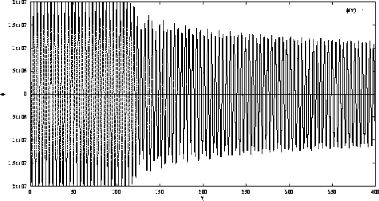
Figure 3.1: Plot of $\phi$ vs $\eta$, with $\text{$M_{\text{{\tiny P}}}$}/m=1.0\times 10^{14}$.

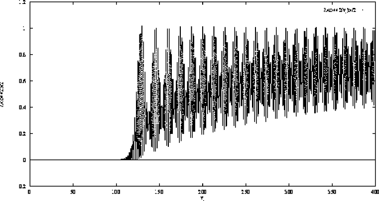
Figure 3.2: Plot of $\lambda\langle\text{$\varphi$}^{2}\rangle/2$ vs $\eta$, with $\text{$M_{\text{{\tiny P}}}$}/m=1.0\times 10^{14}$.

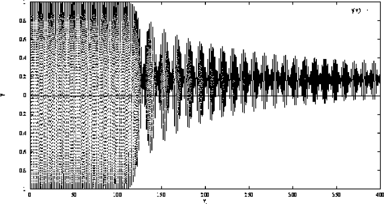
Figure 3.3: Plot of $\gamma$ vs $\eta$, with $\text{$M_{\text{{\tiny P}}}$}/m=1.0\times 10^{14}$.

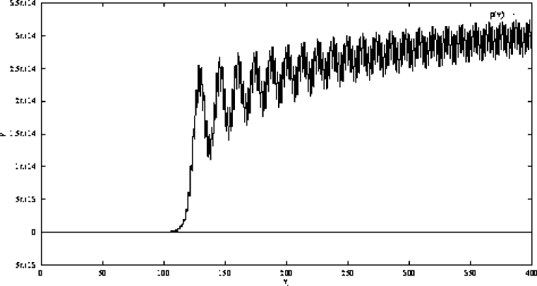
Figure 3.4: Plot of $\rho_{\text{{\tiny Q}}}$ vs $\eta$, with $\text{$M_{\text{{\tiny P}}}$}/m=1.0\times 10^{14}$.

The different solutions plotted correspond to different values of $\text{$M_{\text{{\tiny P}}}$}/m$, with $\lambda=10^{-14}$, $K/m=50$, and $\phi(\eta_{0})/m=2.0\times 10^{7}$. As discussed in Sec. 3.4.2, a physical momentum cutoff $K$ was used. The values chosen for $\text{$M_{\text{{\tiny P}}}$}/m$ were $10^{14}$, $10^{12}$, $6\times 10^{10}$, and $6\times 10^{9}$. The choice of $\text{$\hat{\phi}$}(\eta_{0})$ and $\lambda$ fixes $\eta_{0}$ by Eq. (3.33) and $H_{0}$ by Eq. (3.34). Table 3.1 shows (in units where $m=1$) the values of $M_{\text{{\tiny P}}}$, the inverse Hubble constant $H^{-1}(\eta_{0})$, and the figure numbers in which the corresponding solutions are plotted. The $H^{-1}(\eta_{0})$ column is the initial inverse Hubble constant, which gives the initial time scale for cosmic expansion. Figs. 3.1–3.19 plot the resulting solutions.

Figures	$\text{$\hat{\phi}$}(\eta_{0})$	$\lambda$	$M_{\text{{\tiny P}}}$	$K$	$H^{-1}(\eta_{0})$
3.1–3.4	$2\times 10^{7}$	$1\times 10^{-14}$	$1\times 10^{14}$	50.0	$1.7275\times 10^{6}$
3.5–3.8	$2\times 10^{7}$	$1\times 10^{-14}$	$1\times 10^{12}$	50.0	$1.7275\times 10^{4}$
3.9–3.14	$2\times 10^{7}$	$1\times 10^{-14}$	$6\times 10^{10}$	50.0	$1.0364\times 10^{3}$
3.15–3.19	$2\times 10^{7}$	$1\times 10^{-14}$	$6\times 10^{9}$	50.0	103.65

Table 3.1: Values of parameters for numerical solutions of Eqs. (3.75), (3.83), (3.76).

The time scales defined in Sec. 3.2.4 can now be explicitly computed. Using Eqs. (3.37) and (3.34), we have $f(\eta_{0})=\sqrt{2}$, $\rho_{0}=\text{$\hat{\phi}$}^{2}_{0}$, and

$$H(\eta_{0})=\sqrt{\frac{8\pi\text{$\hat{\phi}$}_{0}^{2}}{3\text{$M_{\text{{\tiny P}}}$}^{2}}}\equiv H_{0}.$$ (3.98)

Using Eq. (3.36), we find $\tau_{0}\simeq 4.118\,32\;m^{-1}$. The value of $\tau_{1}$ predicted by Eq. (3.41) is 132.624 $m^{-1}$, which is very close to the value predicted by Eq. (3.43), 132.759 $m^{-1}$. For the cases $\text{$M_{\text{{\tiny P}}}$}/m=10^{14}$ and $10^{12}$, it is clear from Table 3.1 that $H^{-1}_{0}\gg\tau_{1}$, so that the effect of cosmic expansion is expected to be insignificant on the preheating time scale $\tau_{1}$. For the case $\text{$M_{\text{{\tiny P}}}$}=6\times 10^{10}$, $1/(H_{0}\tau_{1})\sim 7.8$, so that the effect of cosmic expansion should be apparent and non-negligible. For the case $\text{$M_{\text{{\tiny P}}}$}=6\times 10^{9}$, $1/(H_{0}\tau_{1})\sim 0.78$, and cosmic expansion should have a significant effect on parametric amplification of quantum fluctuations.

Figs. 3.1–3.8 show the dynamics of the mean field and variance in the regime of very weak cosmic expansion, $H^{-1}\ll\tau_{1}$.

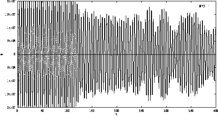
Figure 3.5: Plot of $\phi$ vs $\eta$, with $\text{$M_{\text{{\tiny P}}}$}/m=1.0\times 10^{12}$.

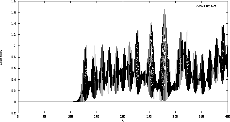
Figure 3.6: Plot of $\lambda\langle\text{$\varphi$}^{2}\rangle/2$ vs $\eta$, with $\text{$M_{\text{{\tiny P}}}$}/m=1.0\times 10^{12}$.

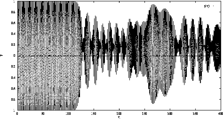
Figure 3.7: Plot of $\gamma$ vs $\eta$, with $\text{$M_{\text{{\tiny P}}}$}/m=1.0\times 10^{12}$.

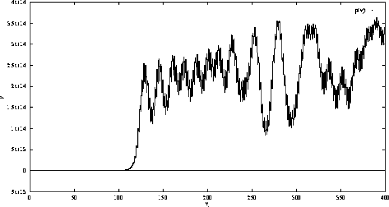
Figure 3.8: Plot of $\rho_{\text{{\tiny Q}}}$ vs $\eta$, with $\text{$M_{\text{{\tiny P}}}$}/m=1.0\times 10^{12}$.

As expected, under the influence of the elliptically oscillating mean field, the variance $\langle\text{$\varphi$}_{\text{{\tiny H}}}^{2}\rangle$ grows exponentially in time until $\lambda\langle\text{$\varphi$}_{\text{{\tiny H}}}^{2}\rangle/2$ is of the same order as $m^{2}+\lambda\text{$\hat{\phi}$}^{2}/2$, at which point back reaction shuts off the resonant transfer of energy to the inhomogeneous modes. The time scale for the variance to become of order unity can be clearly seen to be $\sim\tau_{1}$. As seen previously in studies of preheating dynamics in Minkowski space [99], on the time scale $\sim\tau_{1}$, the mean field decouples from its own fluctuations and oscillates with an asymptotically finite amplitude, given by [99] $\lambda\bar{\text{$\hat{\phi}$}^{2}}/(2m^{2})=0.914$. In the Minkowski space limit, corresponding to $\text{$M_{\text{{\tiny P}}}$}/m\rightarrow\infty$, covariant conservation of the energy-momentum tensor implies that $d{\rho}/dt=0$. This was verified for the case of $\text{$M_{\text{{\tiny P}}}$}/m=10^{14}$, where no change in $\rho$ was detected to within the numerical precision of our algorithm, as expected from dimensional analysis of Eq. (3.83). The increase in the scale factor for these cases was within a few parts in $10^{6}$ of the initial value $a(\eta_{0})=1$. The asymptotic equation of state plotted in Fig 3.13 is observed to be $\bar{\gamma}\sim 0.18$. This is exactly what would be predicted for a two-fluid model consisting of a mean field with equation of state given by Eq. (3.42), $\bar{\gamma}_{\text{{\tiny C}}}\simeq 0.0288$, and a relativistic gas corresponding to the energy density of the $\varphi$ field, with $\bar{\gamma}_{\text{{\tiny Q}}}\simeq 0.3333$. The average $\bar{\gamma}_{\text{{\tiny Q}}}+\bar{\gamma}_{\text{{\tiny C}}}=0.182$.

For the case $\text{$M_{\text{{\tiny P}}}$}/m=6\times 10^{10}$, the effect of cosmic expansion is clearly visible in Figs. 3.9–3.14.

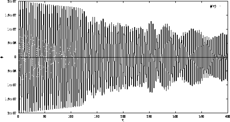
Figure 3.9: Plot of $\phi$ vs $\eta$, with $\text{$M_{\text{{\tiny P}}}$}/m=6.0\times 10^{10}$.

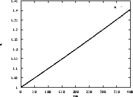
Figure 3.10: Plot of $a$ vs $\eta$, with $\text{$M_{\text{{\tiny P}}}$}/m=6.0\times 10^{10}$.

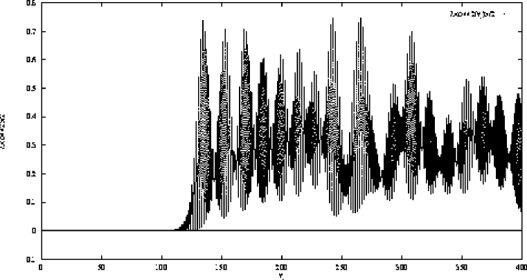
Figure 3.11: Plot of $\lambda\langle\text{$\varphi$}^{2}\rangle/2$ vs $\eta$, with $\text{$M_{\text{{\tiny P}}}$}/m=6.0\times 10^{10}$.

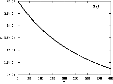
Figure 3.12: Plot of $\rho$ vs $\eta$, with $\text{$M_{\text{{\tiny P}}}$}/m=6.0\times 10^{10}$.

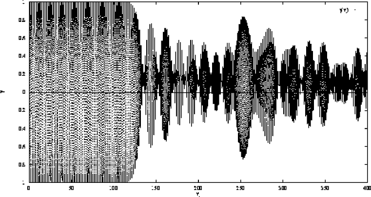
Figure 3.13: Plot of $\gamma$ vs $\eta$, with $\text{$M_{\text{{\tiny P}}}$}/m=6.0\times 10^{10}$.

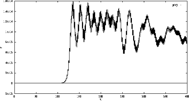
Figure 3.14: Plot of $\rho_{\text{{\tiny Q}}}$ vs $\eta$, with $\text{$M_{\text{{\tiny P}}}$}/m=6.0\times 10^{10}$.

In Fig. 3.9, the coherent oscillations of the mean field for the time period $0<\eta-\eta_{0}<\;\sim 27\tau_{0}$ are clearly seen to be redshifted by the usual $1/a$ factor expected from the Hubble damping term in Eq. (3.75). The expected asymptotic equation of state (taking into account cosmic expansion) computed from a simple two-fluid model is $\sim 0.133$, in agreement with Fig. 3.13.

Figs. 3.15–3.19 show the solution for $\text{$M_{\text{{\tiny P}}}$}/m=6\times 10^{9}$.

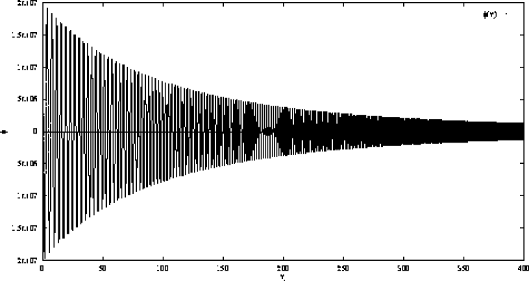
Figure 3.15: Plot of $\phi$ vs $\eta$, with $\text{$M_{\text{{\tiny P}}}$}/m=6.0\times 10^{9}$.

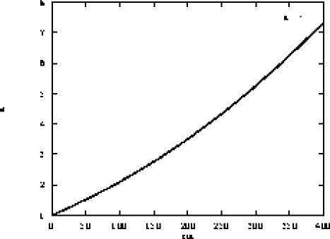
Figure 3.16: Plot of $a$ vs $\eta$, with $\text{$M_{\text{{\tiny P}}}$}/m=6.0\times 10^{9}$.

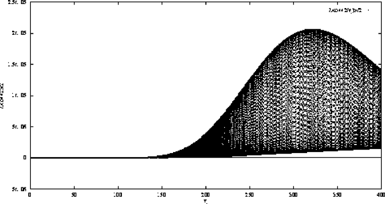
Figure 3.17: Plot of $\lambda\langle\text{$\varphi$}^{2}\rangle/2$ vs $\eta$, with $\text{$M_{\text{{\tiny P}}}$}/m=6.0\times 10^{9}$.

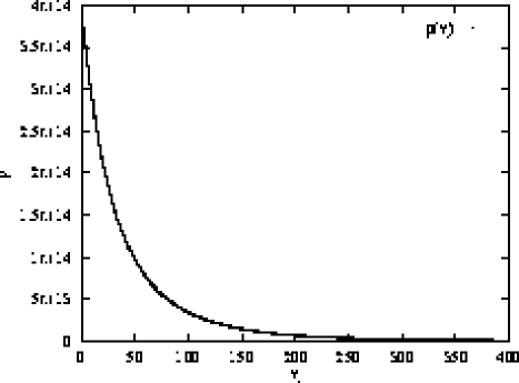
Figure 3.18: Plot of $\rho$ vs $\eta$, with $\text{$M_{\text{{\tiny P}}}$}/m=6.0\times 10^{9}$.

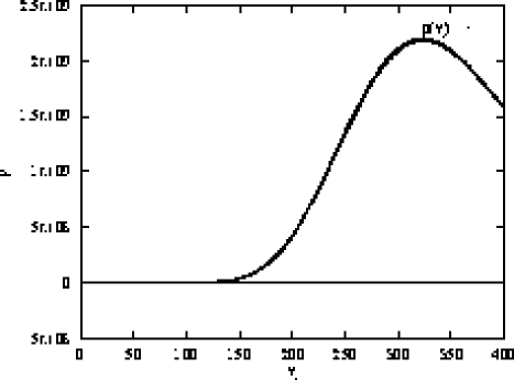
Figure 3.19: Plot of $\rho_{\text{{\tiny Q}}}$ vs $\eta$, with $\text{$M_{\text{{\tiny P}}}$}/m=6.0\times 10^{9}$.

In this case, $1/(H_{0}\tau_{1})\sim 0.781$. From Fig. 3.17, we clearly see that cosmic expansion renders parametric amplification of quantum fluctuations an inefficient mechanism of energy transfer to the inhomogeneous modes. The very rapid oscillations of the mean field at late times are due to the conformal time scale used here, in which the oscillation period of the mean field decreases inversely with $a$. Damping of the mean field due to cosmic expansion is the dominant effect in Fig. 3.15. The power-law decrease in energy density consistent with matter having an effective equation of state $\bar{\gamma}\simeq 0.0288$ can be seen in Fig. 3.18. At $\eta=300\;m^{-1}$, the ratio $\rho_{\text{{\tiny Q}}}/\rho\sim 0.0002$, so the fraction of energy density in the inhomogeneous modes is negligible in comparison to the classical, mean-field contribution. Since the variance $\langle\text{$\varphi$}_{\text{{\tiny H}}}^{2}\rangle$ is never large enough that it dominates the effective mass $M$, the mode functions approximately obey the one-loop equation, in which the effective frequency is $k^{2}+a^{2}(m^{2}+\lambda\text{$\hat{\phi}$}^{2})$, neglecting the $a^{\prime\prime}/a$ term. The width of the resonance can then be shown to be approximately given by $k^{2}\leq\lambda\text{$\hat{\phi}$}^{2}_{0}/2$. The variance is damped by $1/a^{2}$ due to cosmic redshift, so when $H^{-1}\sim\tau_{1}$, the variance never grows to be of order unity.

In addition to varying $M_{\text{{\tiny P}}}$, the coupling $\lambda$ was varied, with results in agreement with Eq. (3.41), showing a logarithmic dependence of $\tau_{1}$ on $\lambda^{-1}$.

3.5 Summary

In this Chapter we use the minimally coupled, quartically self-interacting scalar O$(N)$ field theory as a model for the inflaton field, and study its nonequilibrium dynamics nonperturbatively in a spatially flat FRW spacetime whose evolution is driven by the quantum field. We solve the coupled, self-consistent semiclassical Einstein equation, mean-field equation, and conformal-mode-function equations numerically. Our goal in this Chapter is to study the effects of spacetime dynamics on the mean field, and parametric amplification of quantum fluctuations. This process of energy transfer from the mean field to the inhomogeneous modes is inherently nonperturbative and nonequilibrium. It requires the use of the closed-time-path formalism and the two-particle-irreducible effective action. As our focus in this Chapter is on the parametric amplification of quantum fluctuations, we assume unbroken symmetry. Our analysis is, therefore, most relevant to reheating in chaotic inflation scenarios. We use the two-loop, covariant equations for the mean field and the two-point function for the fluctuation field derived in Chapter 2 and study the case of leading order in the $1/N$ expansion, an approximation which is valid on time scales much shorter than the mean-free time for multiparticle scattering ($\tau_{2}$). For FRW spacetimes, we use the well-established adiabatic regularization procedure to obtain finite expressions for the renormalized variance and energy-momentum tensor which enter into the mean-field equation, conformal-mode function equations, and the semiclassical Einstein equation. In our approach, covariant conservation of the energy-momentum tensor is preserved at all times, as it should be. (It should not and need not be put in by hand, as was done in a recent study of reheating in a fixed background FRW spacetime [162].) We use the adiabatic vacuum construction (matched at conformal-past infinity) to define the quantum state for the fluctuation field in FRW spacetime with asymptotic de Sitter initial conditions; this is the most physical vacuum construction given the decidedly nonadiabatic conditions which prevail at the end of inflation. The instantaneous Hamiltonian diagonalization constructions used in earlier studies of reheating in curved spacetime [124, 116] are known to be problematic [130].

We evolved the coupled dynamical equations for the mean field, variance, and scale factor using standard numerical methods, for time scales of 400 $m^{-1}$, where the initial period of mean-field oscillations is 4.11832 $m^{-1}$. Several regimes for the parameters of the system were investigated. From the solutions of the dynamical equations we studied the behavior of the scale factor $a$, the mean field $\hat{\phi}$, the energy density $\rho$, pressure-to-energy-density ratio $\gamma$, and the inhomogeneous-mode (fluctuation-field) energy density $\rho_{\text{{\tiny Q}}}$. The solutions of the dynamical equations were analyzed for a variety of values for $\text{$M_{\text{{\tiny P}}}$}\tau_{0}$, the parameter which controls the rate of cosmic expansion relative to the time scale for mean-field oscillations in the model. In the case of negligible cosmic expansion, corresponding to very small initial inflaton amplitude, the dynamics is identical to that seen in the group 2B (see Sec. 1.2) studies of O$(N)$ preheating in Minkowski space [99]. In particular, the conservation of energy and logarithmic dependence of the preheating time scale $\tau_{1}$ on the inverse coupling $\lambda^{-1}$ [as shown in Eq. (3.41)] are confirmed. For the case of moderate cosmic expansion, $H(\eta_{0})\tau_{1}\sim 10$ [where $H(\eta_{0})$ is the Hubble parameter at the initial time $\eta_{0}$], energy transfer via parametric amplification of quantum fluctuations is still efficient, and the dynamics can be understood using the analytic results of [99] (for Minkowski space), in terms of the conformally transformed mean-field amplitude $\tilde{\text{$\hat{\phi}$}}=\text{$\hat{\phi}$}/a$ and oscillation period $\tilde{\tau}_{0}=\tau_{0}/a$. The asymptotic effective equation of state is found to be consistent with the prediction of a simple two-fluid description of the late-time behavior of the system.

The most significant physical result concerns the case of rapid cosmic expansion, where $H^{-1}(\eta_{0})\simeq\tau_{1}$. In this case we find that parametric amplification of quantum fluctuations (via parametric resonance) is an inefficient mechanism of energy transfer to the inhomogeneous modes of the inflaton, because the parametric resonance effect is inhibited both by redshifting of the mean-field amplitude and by the redshifting of the physical momenta of the modes out of the resonance band. The energy density of particles produced through parametric resonance is in this case redshifted so rapidly that, in our model, the term $\lambda\langle\text{$\varphi$}_{\text{{\tiny H}}}^{2}\rangle/2$ never grows to be of the order of the tree-level effective mass, $m^{2}+\lambda\text{$\hat{\phi}$}^{2}/2$. As the mean-field amplitude is damped ($\propto 1/a$) due to cosmic expansion, eventually the resonant particle production ceases, and the mean field oscillates with a damped envelope at late times. This leads us to the following conclusions: (i) On the physical level, in chaotic inflation scenarios with a $\lambda\Phi^{4}$ inflaton minimally coupled to gravity and with a large initial inflaton amplitude at the end of slow roll, parametric amplification of the inflaton’s own quantum fluctuations is not a viable mechanism for reheating the Universe, unless the self-coupling is significantly increased. This does not imply that the phenomenon of parametric amplification of quantum fluctuations does not play a vital role in the “preheating” period of inflationary cosmology, for different models and/or couplings. The interesting case of a $\phi^{2}\chi^{2}$ model is currently under investigation. (ii) On a more methodological level, we conclude that a correct study of the reheating period in a chaotic inflation model with large inflaton amplitude at the onset of reheating must take into account the effects of spacetime dynamics. This should be carried out self-consistently using the coupled semiclassical Einstein equation and matter-field equations, so that no ad hoc assumptions need be made about the effective equation of state and/or the relevant time scales involved.

A full two-loop treatment of the unbroken symmetry mean-field dynamics of the O$(N)$ field theory [which involves solving the nonlocal, integro-differential equations (2.116) and (2.117)] includes multiparticle scattering processes, which provide a mechanism for reheating; but they are of a qualitatively different nature than the parametric resonance energy-transfer mechanism studied here. In addition, the nonlocal nature of the gap equation in the full two-loop analysis makes numerical solution of the coupled Einstein and matter equations difficult. In our model, scattering occurs on a time scale $\tau_{2}$ which is significantly longer than the time scale $\tau_{1}$ for parametric amplification of quantum fluctuations. Therefore, in this model the leading-order, large-$N$ (collisionless) approximation is sufficient for a study of parametric amplification of quantum fluctuations. In addition, realistic models of inflation invariably involve couplings of the inflaton to other fields, which provides additional mechanisms of energy transfer away from the inflaton mean field, and into its (or other fields’) quantum modes.

The issues involved in a systematic study of the thermalization stage of post-inflationary physics are more complex. A quantum kinetic field theory treatment taking into account multiparticle scattering is required. The two-loop, 2PI effective action is the simplest and most generally applicable rigorous formalism which contains the leading-order multiparticle scattering processes. The leading-order, $1/N$ approximation is a collisionless subcase of the two-loop, 2PI effective action; it is employed in this study in order to obtain local dynamical equations which can be solved numerically, and is adequate for a study of parametric amplification of quantum fluctuations. In addition, the growth of entropy must be understood within the context of a physically meaningful coarse graining of the full time-reversal-invariant quantum dynamics of the field theory. This is discussed in Chapter 5 below. A first-principles analysis of the thermalization stage is currently underway [184].

Chapter 4 Fermion production, noise, and stochasticity

4.1 Introduction

4.1.1 Background and issues

In Chapter 3 we studied the effect of parametric particle creation on the inflaton dynamics in the post-inflation, “preheating” stage. It was shown that analysis of the dominant physical processes during the early stages of reheating necessitates consideration of self-consistent back reaction of the inflaton variance on the mean field and inhomogeneous modes. This is a nonperturbative effect, and its description requires a consistent truncation of the Schwinger-Dyson equations [82, 99, 125]. Assuming initial conditions conducive to efficient parametric particle creation, the end state of the regime of parametric particle creation consists of a large inflaton variance (i.e., on the order of the tree level terms in the inflaton’s effective mass). Thus, both the inflaton mean field and variance should be treated on an equal footing. This requires a two-particle-irreducible (2PI) formulation of the effective action which is a subclass of the master effective action [82].

During the later stages of reheating, the dynamics of the inflaton field is thought, in the case of unbroken symmetry, to be dominated by fermionic particle creation [166]. This stage of inflaton dynamics is the subject of this chapter. We consider a model consisting of a scalar inflaton field $\phi$ (with $\lambda\phi^{4}$ self-coupling) coupled to a spinor field $\psi$ via a Yukawa interaction and we attempt to present as complete and rigorous a treatment as mandated by the self-consistency of the formalism and the actual solvability of the equations. Thus, we adopt a closed-time-path (CTP), two-particle-irreducible (2PI), coarse-grained effective action (CGEA) to derive the dynamics of the inflaton field. We have explained the significance of CTP and 2PI in Chapter 2 [67, 68, 69, 84, 185, 82, 80], and their relevance to the study of inflaton dynamics in Chapter 3. Here, an added feature of an open system is introduced: we wish to include the averaged effect of an environment on the system, and a useful method is via the coarse-grained effective action [186, 187, 188, 189, 190]. Let us explain the rationale for this.

4.1.2 Coarse-Grained Effective Action

In inflationary cosmology at the onset of the reheating period, the inflaton field’s zero mode typically has a large expectation value, whereas all other fields coupled to the inflaton, as well as inflaton modes with momenta greater than the Hubble constant, are to a good approximation in a vacuum state [8]. This suggests imposing a physical coarse graining in which one regards the inflaton field as the system, and the various quantum fields coupled to it as the environment. From the closed-time-path, coarse-grained effective action (CTP-CGEA) [186, 187, 188, 189, 190] derived in Sec. 4.2 below, one obtains effective dynamical equations for the inflaton field, taking into account its effect on the environment, and back reaction therefrom. For the present problem, the system consists of the inflaton mean field and variance, and the environment consists of the spinor field(s) coupled to the system via a Yukawa interaction.

We wish to emphasize here a subtle yet important distinction between the system-environment division in nonequilibrium statistical mechanics and the system-bath division assumed in thermal field theory. In the latter, one assumes that the propagators for the bath degrees of freedom are fixed, finite-temperature equilibrium Green functions, whereas in the case of the CTP-CGEA, the environmental propagators are slaved (in the sense of [82]) to the dynamics of the system degrees of freedom, and are not fixed a priori to be equilibrium Green functions for all time. This distinction is important for discussions of fermion particle production during reheating, because it is only when the inflaton mean field amplitude is small enough for the use of perturbation theory, that the system-bath split implicit in thermal field theory can be used. Otherwise, one must take into account the effect of the inflaton mean field on the bath (spinor) propagators.

4.1.3 Earlier work

The first studies of particle production during reheating in inflationary cosmology were [91, 93], where reasonable estimates of particle production were made, but back reaction effects were not addressed. The earliest studies of fermionic particle creation during reheating used time-dependent perturbation theory to compute the imaginary part of the self-energy for the zero mode of the inflaton field, which was related to the damping parameter in a friction-type phenomenological term in the equation of motion for the inflaton zero mode [91, 92, 191, 94, 95]. In these studies, it was assumed that the effect of fermionic particle production on the dynamics of the inflaton zero mode is that of a $\Gamma\dot{\phi}$ friction term. However, it has been shown [192, 69, 106, 107, 87, 108, 112, 90] that this assumption is not tenable for a wide variety of field-theoretic interactions and initial conditions. Rather, the effect of back reaction from particle production must be accounted for by deriving the effective evolution equation for the quantum expectation value of the inflaton zero mode, where the dynamics of the degrees of freedom of the produced particles are either coarse-grained (as in Sec. 4.3), or accounted for through self-consistent coupled equations (as in Sec. 4.2). In general, particle creation leads to a nonlocal dissipation term in the inflaton mean field equation, and it is only under rather idealized conditions and specialized cases that one can expect the dissipation kernel to approach a delta function (i.e., a friction term) [74, 75, 53, 56]. Therefore, [91, 94, 95] missed the time-nonlocal nature of fermion particle production and its effect on the dynamics of the inflaton field. In addition, these studies computed the self-energy in flat space, thereby neglecting the effect of curved spacetime on fermion production, and did not examine the stochastic noise arising from the coarse graining of the fermion field.

In addition, most early studies of fermion production during reheating, in using time-dependent perturbation theory to compute the vacuum particle production rate [91, 94, 95], did not include the effect of back reaction of the produced fermion particles on the particle production process itself. In [112], the effect of a thermal initial fermion distribution on the particle production process was investigated (and a Pauli blocking effect was shown), but their analytic derivation of the Pauli blocking effect involves the same perturbative expansion (i.e., system-bath split) described above, and therefore does not incorporate the effect of the produced fermion quanta on the particle production process. In order to take this effect into account, it is necessary to include the effect of the time-varying inflaton mean field in the equation of motion for the spinor propagator, which amounts to a coarse graining of the fermion field, in the system-environment sense, as described above. The perturbative amplitude expansion of the effective inflaton dynamics, in contrast, amounts to a system-bath coarse graining which does not include this back reaction effect.

More recent studies of fermion production during reheating [110, 111, 112] obtained dynamical equations for the inflaton mean field using a one-loop factorization of the Lagrangian, and solved them numerically. However, these studies were carried out in flat space, and because they studied only the dynamics of the inflaton mean field (and at one loop), their analysis did not take into account the back reaction of the inflaton variance on the fermion quantum modes, nor the back reaction of particle production on the dynamics of the inflaton two-point function. The importance of the curved spacetime effect was addressed in Chapter 3, and we will discuss below the importance of treating the inflaton quantum variance on equal footing with the mean field.

4.1.4 Present work

In this study, we wish to describe the late stages of the reheating period, in which the damping of the inflaton mean field is dominated by fermionic particle production; our starting point is the end of the preheating period (in which the inflaton dynamics was dominated by back reaction from parametric particle creation, as discussed in Chapter 3. Because the inflaton variance $\langle\varphi^{2}\rangle$ can (for sufficiently strong self-coupling) be on the order of the square of the amplitude of mean field oscillations at the end of preheating (in the case of unbroken symmetry) [125], it is necessary to treat the inflaton mean field and variance on an equal footing in a study of the subsequent effective dynamics of the inflaton field. This requires a two-loop, two-particle-irreducible formulation of the coarse-grained effective action. At two loops, both the inflaton mean field and the inflaton variance couple to the spinor degrees of freedom, and are damped by back reaction from fermion particle production; all the previous studies mentioned above, in using the 1PI effective action, missed this possibly important effect.

In addition to having a large variance, the inflaton amplitude at the end of the preheating period may be large enough that the usual perturbative expansion in powers of the Yukawa coupling constant is not valid [see Eq. (4.49) below], in which case a nonperturbative derivation of the inflaton dynamics is required. In the construction of the CTP-2PI, coarse-grained effective action below, the spinor propagators obey one-loop dynamical equations in which the inflaton mean field acts as an external source. Studies of fermion particle production during reheating which relied on the use of perturbation theory in the Yukawa coupling constant [91, 93, 92, 191, 94, 95, 87] therefore do not apply to the case of fermion particle production at the end of preheating with unbroken symmetry, when the Yukawa coupling is sufficiently large. The dynamical equations derived in Sec. 4.2 below for the inflaton mean field and variance are applicable even when, as may be the case, the inflaton mean field amplitude is large enough that a perturbative expansion in powers of the Yukawa coupling is not justified.

Although, as discussed above, a proper treatment of the early stage of fermion production during reheating, starting at the end of preheating with unbroken symmetry, should in principle employ the CTP-2PI-CGEA to obtain coupled equations of motion for the inflaton mean field and variance, at very late times the inflaton mean field and variance will have been damped sufficiently (due to the dissipative mechanisms derived below in Sec. 4.2) that the perturbative 1PI effective action will yield a qualitatively correct description of the inflaton mean-field dynamics. While curved spacetime effects should in principle be incorporated self-consistently for a quantitative calculation of the reheating temperature in a particular inflationary model (as discussed in [125]), for a general discussion of dissipative effective dynamics of the inflaton mean field in the case of weak cosmic expansion (where the Hubble constant $H$ is much smaller than the frequency of inflaton oscillations), it is reasonable to neglect curved spacetime effects in computing the spinor propagators. Therefore in Sec. 4.3, we derive the perturbative, flat-space CTP-1PI-CGEA to fourth order in the Yukawa coupling constant, and obtain an evolution equation for the inflaton mean field with nonlocal dissipation.

Another new feature of our work obtainable only from the stochastic approach adopted here is the derivation, in Sec. 4.4, of a Langevin equation for the inflaton mean field, with clear identification of the dissipation and noise kernels from the CGEA. We have calculated the energy dissipated and the fluctuations in the energy. From the latter we obtain the range of parameters where the conventional “mean-field” approach breaks down. We believe the methodology presented here provides a better theoretical framework for the investigation of phase transitions in the early universe, as exemplified by our treatment of reheating in inflationary cosmology.

4.1.5 Organization

Our work is organized as follows. In Sec. 4.2, we derive the coupled equations of motion for the inflaton mean field and variance, in a general curved spacetime, including diagrams in the coarse-grained CTP-2PI effective action of up to two-loop order. In Sec. 4.3, we specialize to Minkowski space and small mean-field amplitude, and obtain a perturbative mean field equation including dissipative effects up to fourth order in the Yukawa coupling constant. In Sec. 4.4, we examine the dissipation and noise kernels obtained in Sec. 4.3, and show that they obey a fluctuation-dissipation relation. We then derive a Langevin equation which self-consistently includes the effect of noise on the dynamics of the inflaton zero mode. We summarize our results in Sec. 4.5.

4.2 Coarse-grained inflaton dynamics in curved spacetime

In this section, we present a first-principles derivation of the nonequilibrium, nonperturbative, effective dynamics of a scalar inflaton field $\phi$ coupled to a spinor field $\psi$ via a Yukawa interaction, in a general, curved classical background spacetime. The use of the Schwinger-Keldysh closed-time-path (CTP) formalism allows formulation of the nonequilibrium dynamics of the inflaton from an appropriately defined initial quantum state. The evolution equations for the inflaton mean field and variance are derived from the two-loop, closed-time-path (CTP), two-particle-irreducible (2PI), coarse-grained effective action (CGEA). As the name suggests, there are two approximations of a statistical mechanical nature. One is the coarse graining of the environment— here the inflaton field is the system and the fermion field is the environment [186]. The other refers to a truncation of the correlation hierarchy for the inflaton field [82]— the two-particle-irreducible effective action. This formulation retains the inflaton mean field and variance as coupled dynamical degrees of freedom. Back Reaction of the scalar and spinor field dynamics on the spacetime is incorporated using the semiclassical Einstein equation, which follows from functional differentiation of the effective action with respect to the metric. It is shown that these dynamical equations are both real and causal, and the equations are cast in a form suitable for implementation of an explicit curved-spacetime renormalization procedure.

4.2.1 The model

We study a model consisting of a scalar field $\phi$ (the inflaton field) which is Yukawa-coupled to a spinor field $\psi$, in a curved, dynamical, classical background spacetime. The total action

$$S[\phi,\bar{\psi},\psi,g^{\mu\nu}]=S^{\text{{\tiny G}}}[g^{\mu\nu}]+S^{\text{{\tiny F}}}[\phi,\bar{\psi},\psi,g^{\mu\nu}],$$ (4.1)

consists of a part depicting classical gravity, $S^{\text{{\tiny G}}}[g^{\mu\nu}]$, and a part for the matter fields,

$$S^{\text{{\tiny F}}}[\phi,\bar{\psi},\psi,g^{\mu\nu}]=S^{\phi}[\phi,g^{\mu\nu}]+S^{\psi}[\bar{\psi},\psi,g^{\mu\nu}]+S^{\text{{\tiny Y}}}[\phi,\bar{\psi},\psi,g^{\mu\nu}],$$ (4.2)

whose scalar (inflaton), spinor (fermion), and Yukawa-interaction parts are given by

$$S^{\phi}[\phi,g^{\mu\nu}]=-\frac{1}{2}\int d^{\;4}x\sqrt{-g}\left[\phi(\square+m^{2}+\xi R)\phi+\frac{\lambda}{12}\phi^{4}\right],$$ (4.3)

$$S^{\psi}[\bar{\psi},\psi,g^{\mu\nu}]=\int d^{\;4}x\sqrt{-g}\left[\frac{i}{2}\left(\bar{\psi}\gamma^{\mu}\nabla_{\mu}\psi-(\nabla_{\mu}\bar{\psi})\gamma^{\mu}\psi\right)-\mu\bar{\psi}\psi\right],$$ (4.4)

$$S^{\text{{\tiny Y}}}[\phi,\bar{\psi},\psi,g^{\mu\nu}]=-\text{$f$}\int d^{\;4}x\sqrt{-g}\phi\bar{\psi}\psi.$$ (4.5)

For this theory to be renormalizable in semiclassical gravity, the bare gravity action $S^{\text{{\tiny G}}}[g^{\mu\nu}]$ of Eq. (4.1) should have the form given by Eq. (2.65) [129, 17]. In Eqs. (4.3)–(4.5), $m$ is the scalar field “mass” (with dimensions of inverse length); $\xi$ is the dimensionless coupling to gravity; $\mu$ is the spinor field “mass,” with dimensions of inverse length; $\square$ is the Laplace-Beltrami operator in the curved background spacetime with metric tensor $g_{\mu\nu}$; $\nabla_{\mu}$ is the covariant derivative compatible with the metric; $\sqrt{-g}$ is the square root of the absolute value of the determinant of the metric; $\lambda$ is the self-coupling of the inflaton field, with dimensions of $1/\sqrt{\hbar}$; $f$ is the Yukawa coupling constant, which has dimensions of $1/\sqrt{\hbar}$; and $R$ is the scalar curvature. The curved spacetime Dirac matrices $\gamma^{\mu}$ satisfy the anticommutation relation

$$\left\{\gamma^{\mu},\gamma^{\nu}\right\}_{+}=2g^{\mu\nu}1_{\text{{\tiny sp}}},$$ (4.6)

in terms of the contravariant metric tensor $g^{\mu\nu}$. The symbol $1_{\text{{\tiny sp}}}$ denotes the identity element in the Dirac algebra.

It is assumed that there is a definite separation of time scales between the stage of “preheating” discussed in Chapter 3, and fermionic particle production, which is our primary focus in this work. However, this does not imply that perturbation theory in the Yukawa coupling constant $f$ is necessarily valid, which would require that condition (4.49) (defined in Sec. 4.3 below) be satisfied. In addition, the fermion field mass $\mu$ is assumed to be much lighter than the inflaton field mass $m$, i.e., the renormalized parameters $m$ and $\mu$ satisfy $m\gg\mu$.

4.2.2 Closed-time-path, coarse-grained effective action

We denote the quantum Heisenberg field operators of the scalar field $\phi$ and the spinor field $\psi$ by $\Phi_{\text{{\tiny H}}}$ and $\Psi_{\text{{\tiny H}}}$, respectively, and the quantum state by $|\Omega\rangle$. For consistency with the truncation of the correlation hierarchy at second order, we assume $\Phi_{\text{{\tiny H}}}$ to have a Gaussian moment expansion in the position basis [150, 118], in which case the relevant observables are the scalar mean field $\hat{\phi}$ [defined in Eq. (3.2)], the mean-squared fluctuations, or variance [defined in Eq. (3.4)]. As discussed above, at the end of the preheating period, the inflaton variance can be as large as the square of the amplitude of mean-field oscillations. On the basis of our assumption of separation of time scales in Sec. 4.2.1, and the conditions which prevail at the onset of reheating, the initial quantum state $|\Omega\rangle$ is assumed to be an appropriately defined vacuum state for the spinor field.

The construction of the CTP-2PI-CGEA for the $\phi\text{$\bar{\psi}$}\psi$ theory in a general, curved, background spacetime closely parallels the construction of the CTP-2PI effective action for the O($N$) model in curved spacetime discussed in Chapter 2. Following the approach of Sec. 2.4, we define a “CTP manifold” ${\mathcal{M}}$, and a volume form ${\boldsymbol{\epsilon}}_{\mathcal{M}}$ on ${\mathcal{M}}$, in terms of the discrete set $\{+,-\}$ labeling the “time branch,” and a Cauchy hypersurface $\Sigma_{\star}$ which is far to the future of the time scales in which we are interested. The spacetime manifold $M$ is the past domain of dependence of $\Sigma_{\star}$. The restrictions of a function $\phi$, defined on ${\mathcal{M}}$, to the $+$ and $-$ time branches are denoted by $\phi_{+}$ and $\phi_{-}$, respectively. We can then define a matter field action on ${\mathcal{M}}$,

$${\mathcal{S}}^{\text{{\tiny F}}}[\phi_{-},\text{$\bar{\psi}$}_{-},\psi_{-},g^{\mu\nu}_{-};\phi_{+},\text{$\bar{\psi}$}_{+},\psi_{+},g^{\mu\nu}_{+}]\equiv S^{\text{{\tiny F}}}[\phi_{+},\text{$\bar{\psi}$}_{+},\psi_{+},g^{\mu\nu}_{+}]-S^{\text{{\tiny F}}}[\phi_{-},\text{$\bar{\psi}$}_{-},\psi_{-},g^{\mu\nu}_{-}],$$ (4.7)

where the spacetime integrations in $S^{\text{{\tiny F}}}$ are now over $M$ only. We use the symbol ${\mathcal{S}}^{\text{{\tiny F}}}$ to distinguish it from the action $S^{\text{{\tiny F}}}$ on $M$. Let us also simplify notation by suppressing time branch indices in the argument of functionals on ${\mathcal{M}}$, i.e.,

$${\mathcal{S}}^{\text{{\tiny F}}}[\phi,\text{$\bar{\psi}$},\psi,g^{\mu\nu}]\equiv{\mathcal{S}}^{\text{{\tiny F}}}[\phi_{-},\text{$\bar{\psi}$}_{-},\psi_{-},g^{\mu\nu}_{-};\phi_{+},\text{$\bar{\psi}$}_{+},\psi_{+},g^{\mu\nu}_{+}].$$ (4.8)

Let us also define the functional ${\mathcal{S}}^{\text{{\tiny Y}}}$ on ${\mathcal{M}}$ by

$${\mathcal{S}}^{\text{{\tiny Y}}}[\phi,\text{$\bar{\psi}$},\psi,g^{\mu\nu}]\equiv S^{\text{{\tiny Y}}}[\phi_{+},\text{$\bar{\psi}$}_{+},\psi_{+},g^{\mu\nu}_{+}]-S^{\text{{\tiny Y}}}[\phi_{-},\text{$\bar{\psi}$}_{-},\psi_{-},g^{\mu\nu}_{-}],$$ (4.9)

in analogy with Eq. (4.7). For a function $\phi$ on ${\mathcal{M}}$, the restrictions of $\phi$ to the $+$ and $-$ time branches are subject to the boundary condition

$$(\phi_{+})_{|\Sigma_{\star}}=(\phi_{-})_{|\Sigma_{\star}}$$ (4.10)

at the hypersurface $\Sigma_{\star}$. The gravity action $S^{\text{{\tiny G}}}$, promoted to a functional on ${\mathcal{M}}$, takes the form

$${\mathcal{S}}^{\text{{\tiny G}}}[g^{\mu\nu}_{+},g^{\mu\nu}_{-}]=S^{\text{{\tiny G}}}[g^{\mu\nu}_{+}]-S^{\text{{\tiny G}}}[g^{\mu\nu}_{-}],$$ (4.11)

where the range of spacetime integration in $S^{\text{{\tiny G}}}$ on the right-hand side of Eq. (4.11) is understood to be over $M$.

To formulate the CTP-2PI-CGEA, our first step is to define a generating functional for $n$-point functions of the scalar field, in terms of the initial quantum state $|\Omega\rangle$ which evolves under the influence of a local source $J$, and a non-local source $K$ coupled to the scalar field (in the interaction picture with the external sources being treated as the “interaction”). This generating functional depends on both $J$ and $K$, as well as the classical background metric $g^{\mu\nu}$. In the path integral representation, the generating functional $Z[J,K,g^{\mu\nu}]$ takes the form of a sum over scalar field configurations $\phi$ and complex Grassmann-valued configurations $\psi$ on the manifold ${\mathcal{M}}$,

$$\begin{split}Z[J,K,g^{\mu\nu}]\equiv\int_{\text{{\tiny ctp}}}&D\phi_{-}D\bar{\psi}_{-}D\psi_{-}D\phi_{+}D\bar{\psi}_{+}D\psi_{+}\exp\Biggl{[}\frac{i}{\hbar}\biggl{(}{\mathcal{S}}^{\text{{\tiny F}}}[\phi,\bar{\psi},\psi,g^{\mu\nu}]\\ &+\int_{M}d^{\;4}x\sqrt{-g}c^{ab}J_{a}\phi_{b}\\ &+\frac{1}{2}\int_{M}d^{\;4}x\sqrt{-g}\int_{M}d^{\;4}x^{\prime}\sqrt{-g^{\prime}}c^{ab}c^{cd}K_{ac}(x,x^{\prime})\phi_{b}(x)\phi_{d}(x^{\prime})\biggr{)}\Biggr{]},\end{split}$$ (4.12)

where $J_{a}(x)$ is a local $c$-number source and $K_{ab}(x,x^{\prime})$ is a nonlocal $c$-number source. The subscript CTP on the functional integral denotes a summation over field configurations $\phi_{\pm}$, $\text{$\bar{\psi}$}_{\pm}$, and $\psi_{\pm}$ which satisfy the boundary condition (4.10). The latin indices $a$, $b$, $c$, $\ldots\;$, have the discrete index set $\{+,-\}$, and denote the time branch [67, 68]. The boundary conditions on the functional integral of Eq. (4.12) at the initial data surface determine the quantum state $|\Omega\rangle$. The CTP indices have been dropped from $g^{\mu\nu}$ for ease of notation; it will be clear how to reinstate them [80] in the two-loop CTP–2PI effective action shown below in Sec. 4.3. The two-index symbol $c^{ab}$ is defined by the $n=2$ case of Eq. (2.27). The generating functional for normalized $n$-point functions is

$$W[J,K,g^{\mu\nu}]=-i\hbar\text{ln}Z[J,K,g^{\mu\nu}],$$ (4.13)

in terms of which we can define the classical scalar field on ${\mathcal{M}}$,

$$\text{$\hat{\phi}$}_{a}(x)_{\text{{\tiny$JK$}}}=c_{ab}\frac{1}{\sqrt{-g}}\frac{\delta W[J,K,g^{\mu\nu}]}{\delta J_{b}(x)},$$ (4.14)

and the scalar two-point function on ${\mathcal{M}}$ in the presence of the sources $J_{a}$ and $K_{ab}$,

$$\hbar G_{ab}(x,x^{\prime})_{\text{{\tiny$JK$}}}=2c_{ac}c_{bd}\frac{1}{\sqrt{-g}}\frac{1}{\sqrt{-g^{\prime}}}\frac{\delta W[J,Kg^{\mu\nu}]}{\delta K_{cd}(x,x^{\prime})}-\text{$\hat{\phi}$}_{a}(x)\text{$\hat{\phi}$}_{b}(x^{\prime}),$$ (4.15)

where the $JK$ subscripts indicate that $\hat{\phi}$ and $G$ are functionals of the $J_{a}$ and $K_{ab}$ sources. In the limit $J_{a}=K_{ab}=0$, the classical field is the same on the two time branches and it is equivalent to the mean field $\hat{\phi}$, as shown in Eq. (2.43). In the same limit, $G_{ab}$ becomes the CTP propagator for the fluctuation field defined in Eq. (3.3), as shown in Eqs. (2.44)–(2.47). In the coincidence limit $x^{\prime}=x$, all four components (2.44)–(2.47) are equivalent to the variance $\langle\text{$\varphi_{\text{{\tiny H}}}$}^{2}\rangle$ defined in Eq. (3.4). Provided we can invert Eqs. (4.14) and (4.15) to obtain $J_{a}$ and $K_{ab}$ in terms of $\text{$\hat{\phi}$}_{a}$ and $G_{ab}$, the CTP–2PI effective action can be defined as the double Legendre transform (in both $J_{a}$ and $K_{ab}$) of $W[J,K,g^{\mu\nu}]$,

$$\Gamma[\text{$\hat{\phi}$},G,g^{\mu\nu}]=W[J,K,g^{\mu\nu}]-\int_{M}d^{\;4}x\sqrt{-g}c^{ab}J_{a}(x)\text{$\hat{\phi}$}_{b}(x)\\ -\frac{1}{2}\int_{M}d^{\;4}x\sqrt{-g}\int_{M}d^{\;4}x^{\prime}\sqrt{-g^{\prime}}c^{ab}c^{cd}K_{ac}(x,x^{\prime})\left[\hbar G_{bd}(x,x^{\prime})+\text{$\hat{\phi}$}_{b}(x)\text{$\hat{\phi}$}_{d}(x^{\prime})\right].$$ (4.16)

The inverses of Eqs. (4.14) and (4.15) can be obtained by functional differentiation of Eq. (4.16) with respect to $\text{$\hat{\phi}$}_{a}$,

$$\frac{1}{\sqrt{-g}}\frac{\delta\Gamma[\text{$\hat{\phi}$},G,g^{\mu\nu}]}{\delta\text{$\hat{\phi}$}_{a}(x)}\\ =-c^{ab}J_{b}(x)_{\text{{\tiny$\text{$\hat{\phi}$}G$}}}-\frac{1}{2}c^{ab}c^{cd}\int_{M}d^{\;4}x^{\prime}\sqrt{-g^{\prime}}\left[K_{bd}(x,x^{\prime})_{\text{{\tiny$\text{$\hat{\phi}$}G$}}}+K_{db}(x^{\prime},x)_{\text{{\tiny$\text{$\hat{\phi}$}G$}}}\right]\text{$\hat{\phi}$}_{c}(x^{\prime}),$$ (4.17)

and with respect to $G_{ab}$,

$$\frac{1}{\sqrt{-g}}\frac{1}{\sqrt{-g^{\prime}}}\frac{\delta\Gamma[\text{$\hat{\phi}$},G,g^{\mu\nu}]}{\delta G_{ab}(x,x^{\prime})}=-\frac{\hbar}{2}c^{ac}c^{bd}K_{cd}(x,x^{\prime})_{\text{{\tiny$\text{$\hat{\phi}$}G$}}},$$ (4.18)

where the $\text{$\hat{\phi}$}G$ subscript indicates that $K_{ab}$ and $J_{a}$ are functionals of $\text{$\hat{\phi}$}_{a}$ and $G_{ab}$. Inserting Eqs. (4.17) and (4.18) into Eq. (4.16) yields a functional integro-differential equation for the CTP–2PI effective action in terms of $\hat{\phi}$ and $G$ only, so the $JK$ subscripts can be dropped. It is useful to change the variable of functional integration to be the fluctuation field about $\text{$\hat{\phi}$}_{a}$ defined by Eq. (2.33). Performing the change-of-variables $D\phi\rightarrow D\varphi$, the equation for $\Gamma$ is

$$\begin{split}\Gamma[\text{$\hat{\phi}$},G,g^{\mu\nu}]&=\int_{M}d^{\;4}x\int_{M}d^{\;4}x^{\prime}\frac{\delta\Gamma[\text{$\hat{\phi}$},G]}{\delta G_{ba}(x^{\prime},x)}G_{ab}(x,x^{\prime})\\ &-i\hbar\text{ln}\Biggl{\{}\int_{\text{{\tiny ctp}}}D\varphi_{+}D\text{$\bar{\psi}$}_{+}D\psi_{+}D\varphi_{-}D\text{$\bar{\psi}$}_{-}D\psi_{-}\exp\biggl{[}\frac{i}{\hbar}\Bigl{(}{\mathcal{S}}^{\text{{\tiny F}}}[\varphi+\text{$\hat{\phi}$},\text{$\bar{\psi}$},\psi,g^{\mu\nu}]\\ &-\int_{M}d^{\;4}x\frac{\delta\Gamma[\text{$\hat{\phi}$},G,g^{\mu\nu}]}{\delta\text{$\hat{\phi}$}_{a}}\varphi_{a}-\frac{1}{\hbar}\int_{M}d^{\;4}x\int_{M}d^{\;4}x^{\prime}\frac{\delta\Gamma[\text{$\hat{\phi}$},G,g^{\mu\nu}]}{\delta G_{ba}(x^{\prime},x)}\varphi_{a}(x)\varphi_{b}(x^{\prime})\Bigr{)}\biggr{]}\Biggr{\}},\end{split}$$ (4.19)

which has the formal solution

$$\Gamma[\text{$\hat{\phi}$},G,g^{\mu\nu}]={\mathcal{S}}^{\phi}[\text{$\hat{\phi}$}]-\frac{i\hbar}{2}\text{ln}\,\text{det}G_{ab}-i\hbar\text{ln}\,\text{det}F_{ab}+\Gamma_{2}[\text{$\hat{\phi}$},G]\\ +\frac{i\hbar}{2}\int_{M}d^{\;4}x\sqrt{-g}\int_{M}d^{\;4}x^{\prime}\sqrt{-g^{\prime}}{\mathcal{A}}^{ab}(x^{\prime},x)G_{ab}(x,x^{\prime}),$$ (4.20)

where ${\mathcal{A}}^{ab}$ is the second functional derivative of the scalar part of the classical action $S^{\phi}$, evaluated at $\hat{\phi}$,

$$\begin{split}i{\mathcal{A}}^{ab}(x,x^{\prime})&=\frac{1}{\sqrt{-g}}\left(\frac{\delta^{2}{\mathcal{S}}^{\phi}}{\delta\phi_{a}(x)\delta\phi_{b}(x^{\prime})}[\text{$\hat{\phi}$}]\right)\frac{1}{\sqrt{-g^{\prime}}}\\ &=-\left[c^{ab}(\square_{x}+m^{2}+\xi R(x))+c^{abcd}\frac{\lambda}{2}\text{$\hat{\phi}$}_{c}(x)\text{$\hat{\phi}$}_{d}(x)\right]\delta(x-x^{\prime})\frac{1}{\sqrt{-g^{\prime}}}.\end{split}$$ (4.21)

The symbol $F_{ab}$ denotes the one-loop CTP spinor propagator, which is defined by

$$F_{ab}(x,x^{\prime})\equiv{\mathcal{B}}_{ab}^{-1}(x,x^{\prime}),$$ (4.22)

where we are suppressing spinor indices, and the inverse spinor propagator ${\mathcal{B}}^{ab}$ is defined by

$$\begin{split}i{\mathcal{B}}^{ab}(x,x^{\prime})&=\frac{1}{\sqrt{-g}}\left[\frac{\delta^{2}({\mathcal{S}}^{\psi}[\text{$\bar{\psi}$},\psi]+{\mathcal{S}}^{\text{{\tiny Y}}}[\text{$\bar{\psi}$},\psi;\text{$\hat{\phi}$}])}{\delta\psi_{a}(x)\delta\text{$\bar{\psi}$}_{b}(x^{\prime})}\right]\frac{1}{\sqrt{-g^{\prime}}}\\ &=\left[c^{ab}\left(i\gamma^{\mu}\nabla^{\prime}_{\mu}-\mu\right)-c^{abc}\text{$f$}\text{$\hat{\phi}$}_{c}(x^{\prime})\right]\delta(x^{\prime}-x)\frac{1}{\sqrt{-g}}{1}_{\text{{\tiny sp}}}.\end{split}$$ (4.23)

It is clear from Eq. (4.23) that the use of the one-loop spinor propagators in the construction of the CTP-2PI-CGEA represents a nonperturbative resummation in the Yukawa coupling constant, which (as discussed above) goes beyond the standard time-dependent perturbation theory. The boundary conditions which define the inverses of Eqs. (4.21) and (4.23) are the boundary conditions at the initial data surface in the functional integral in Eq. (4.12), which in turn, define the initial quantum state $|\Omega\rangle$. The one-loop spinor propagator $F_{ab}$ is related to the expectation values of the spinor Heisenberg field operators for a spinor field in the presence of the c-number background field $\hat{\phi}$,

$$\hbar\left.F_{++}(x,x^{\prime})\right|_{\text{$\hat{\phi}_{+}$}=\text{$\hat{\phi}_{-}$}=\text{$\hat{\phi}$}}=\langle\Omega|T(\text{$\Psi_{\text{{\tiny H}}}$}(x)\text{$\bar{\Psi}_{\text{{\tiny H}}}$}(x^{\prime}))|\Omega\rangle,$$ (4.24)

$$\hbar\left.F_{--}(x,x^{\prime})\right|_{\text{$\hat{\phi}_{+}$}=\text{$\hat{\phi}_{-}$}=\text{$\hat{\phi}$}}=\langle\Omega|\tilde{T}(\text{$\Psi_{\text{{\tiny H}}}$}(x)\text{$\bar{\Psi}_{\text{{\tiny H}}}$}(x^{\prime}))|\Omega\rangle,$$ (4.25)

$$\hbar\left.F_{+-}(x,x^{\prime})\right|_{\text{$\hat{\phi}_{+}$}=\text{$\hat{\phi}_{-}$}=\text{$\hat{\phi}$}}=-\langle\Omega|\text{$\bar{\Psi}_{\text{{\tiny H}}}$}(x^{\prime})\text{$\Psi_{\text{{\tiny H}}}$}(x)|\Omega\rangle,$$ (4.26)

$$\hbar\left.F_{-+}(x,x^{\prime})\right|_{\text{$\hat{\phi}_{+}$}=\text{$\hat{\phi}_{-}$}=\text{$\hat{\phi}$}}=\langle\Omega|\text{$\Psi_{\text{{\tiny H}}}$}(x)\text{$\bar{\Psi}_{\text{{\tiny H}}}$}(x^{\prime})|\Omega\rangle,$$ (4.27)

where the spinor Heisenberg field operators obey the equations

$$(i\gamma^{\mu}\nabla_{\mu}-\mu-f\text{$\hat{\phi}$})\Psi=0,$$ (4.28)

$$(-i\gamma^{\mu}\nabla_{\mu}-\mu-f\text{$\hat{\phi}$})\bar{\Psi}=0.$$ (4.29)

The CTP spinor propagator components satisfy the relations (valid only when $\text{$\hat{\phi}_{+}$}=\text{$\hat{\phi}_{-}$}=\text{$\hat{\phi}$}$)

$$F_{++}(x,x^{\prime})^{\dagger}=F_{--}(x^{\prime},x),$$ (4.30)

$$F_{--}(x,x^{\prime})^{\dagger}=F_{++}(x^{\prime},x),$$ (4.31)

$$F_{-+}(x,x^{\prime})^{\dagger}=F_{-+}(x^{\prime},x),$$ (4.32)

$$F_{+-}(x,x^{\prime})^{\dagger}=F_{+-}(x^{\prime},x).$$ (4.33)

The functional $\Gamma_{2}[\text{$\hat{\phi}$},G]$ is defined as $-i\hbar$ times the sum of all vacuum diagrams drawn according to the following rules:

1. Vertices carry spacetime ($x\in M$) and time branch ($a\in\{+,-\}$) labels.

2. Scalar field lines denote $\hbar G_{ab}(x,x^{\prime})$.

3. Spinor lines denote the one-loop CTP spinor propagator $\hbar F_{ab}(x,x^{\prime})$ (spinor indices are suppressed), defined in Eq. (4.22).

4. There are three interaction vertices, given by $i{\mathcal{S}}^{\text{{\tiny I}}}/\hbar$, which is defined by

   $${\mathcal{S}}^{\text{{\tiny I}}}[\text{$\hat{\phi}$},\varphi,\text{$\bar{\psi}$},\psi]=S^{\text{{\tiny I}}}[\text{$\hat{\phi}_{+}$},\text{$\varphi_{+}$},\text{$\bar{\psi}_{+}$},\text{$\psi_{+}$}]-S^{\text{{\tiny I}}}[\text{$\hat{\phi}_{-}$},\text{$\varphi_{-}$},\text{$\bar{\psi}_{-}$},\text{$\psi_{-}$}],$$ (4.34)

   $$S^{\text{{\tiny I}}}[\text{$\hat{\phi}$},\text{$\varphi$},\text{$\bar{\psi}$},\psi]=-\int d^{4}x\sqrt{-g}\left[f\text{$\varphi$}\text{$\bar{\psi}$}\psi+\frac{\lambda}{24}\text{$\varphi$}^{4}+\frac{\lambda}{6}\text{$\hat{\phi}$}\text{$\varphi$}^{3}\right],$$ (4.35)

   where we have followed the notation of Eq. (4.9).

5. Only diagrams which are two-particle-irreducible with respect to cuts of scalar lines contribute to $\Gamma_{2}$.

The distinction between the CTP-2PI, coarse-grained effective action which arises here, and the fully two-particle-irreducible effective action (2PI with respect to scalar and spinor cuts), is due to the fact that we only Legendre-transformed sources coupled to $\phi$; i.e., the spinor field is treated as the environment. In Eq. (4.21), the curved-spacetime Dirac $\delta$ function is defined as in [17]. Comparison of Eq. (4.20) above with Eq. (4.13) of Ref. [80] [which was computed for the $O(N)$ model] shows that the $\text{Tr}\,\text{ln}F_{ab}$ in Eq. (4.20) differs from the usual one-loop term by a factor of 2, owing to the difference (in the exponent) between the Gaussian integral formulas for real and complex fields [79].

The functional $\Gamma_{2}[\text{$\hat{\phi}$},G,g^{\mu\nu}]$ can be evaluated in a loop expansion, which corresponds to an expansion in powers of $\hbar$,

$$\Gamma_{2}[\text{$\hat{\phi}$},G,g^{\mu\nu}]=\sum_{l=2}^{\infty}\hbar^{l}\Gamma^{(l)}[\text{$\hat{\phi}$},G,g^{\mu\nu}],$$ (4.36)

starting with the two-loop term, $\Gamma^{(2)}$. The functional $\Gamma^{(2)}$ has a diagrammatic expansion shown in Fig. 4.1,

Figure 4.1: Diagrammatic expansion for $\Gamma^{(2)}$, the two-loop part of the CTP-2PI coarse-grained effective action.

where solid lines represent the spinor propagator $F$ (as defined in Sec. 4.2), and dotted lines represent the scalar propagator $G$. The vertices terminating three $\phi$ lines are proportional to the scalar mean field $\hat{\phi}$. Each vertex carries spacetime $(x)$ and CTP $(+,-)$ labels. The $\lambda\phi^{4}$ self-interaction leads to two terms in the two-loop part of the effective action, the second and third graphs of Fig. 4.1. They are the “setting sun” diagram, which is $O(\lambda^{2})$, and the “double bubble,” which is $O(\lambda)$, respectively. The Yukawa interaction leads to only one diagram in $\Gamma^{(2)}$, the first diagram of Fig. 4.1,

$$\frac{if^{2}}{2}c^{aa^{\prime}a^{\prime\prime}}c^{bb^{\prime}b^{\prime\prime}}\int d^{\,4}x\sqrt{-g}\int d^{\,4}x^{\prime}\sqrt{-g^{\prime}}G_{ab}(x,x^{\prime})\text{Tr}_{\text{{\tiny sp}}}\left[F_{a^{\prime}b^{\prime}}(x,x^{\prime})F_{b^{\prime\prime}a^{\prime\prime}}(x^{\prime},x)\right],$$ (4.37)

where the trace is understood to be over the spinor indices which are not shown, and the three-index symbol $c^{abc}$ is defined by the $n=3$ case of Eq. (2.27). Here, we treat the $\lambda$ self-interaction using the time-dependent Hartree-Fock approximation [79], which is equivalent to retaining the $O(\lambda)$ (double-bubble) graph and dropping the $O(\lambda^{2})$ (setting sun) graph. We assume for the present study that the coupling $\lambda$ is sufficiently small that the $O(\lambda^{2})$ diagram is unimportant on the time scales of interest in the fermion production regime of the inflaton dynamics. The mean-field and gap equations including both the $O(\lambda)$ and the $O(\lambda^{2})$ diagrams were derived for a general curved spacetime in Chapter 2.

4.2.3 Evolution equations for $\hat{\phi}$ and $G$ in curved spacetime

The (bare) semiclassical field equations for the two-point function, mean field, and metric can be obtained from the CTP-2PI-CGEA by functional differentiation with respect $G_{ab}$, $\text{$\hat{\phi}$}_{a}$, and $g^{\mu\nu},$ followed by identifications of $\hat{\phi}$ and $g^{\mu\nu}$ on the two time branches, as shown in Eqs. (2.81)–(2.83). These equations constitute the semiclassical approximation to the full quantum dynamics for the system described by the classical action (4.1). Equation (2.81) should be understood as following after time branch indices have been reinstated on the metric tensor in the CTP-2PI-CGEA [80]. The field equation of semiclassical gravity (with bare parameters) is obtained directly from Eq. (2.83), and given by Eq. (2.84). The right-hand side of Eq. (2.84) is the (unrenormalized) quantum energy-momentum tensor defined by Eq. (2.85). The energy-momentum tensor $\langle T_{\mu\nu}\rangle$ is divergent in four spacetime dimensions, and must be regularized via a covariant procedure [17], as discussed in Sec. 3.3.3 above.

Making the two-loop approximation to the CTP-2PI-CGEA, where we take $\Gamma_{2}\simeq\hbar^{2}\Gamma^{(2)}$, and dropping the $O(\lambda^{2})$ diagram from $\Gamma_{2}$, the mean-field equation becomes

$$\left(\square+m^{2}+\xi R(x)+\frac{\lambda}{6}\text{$\hat{\phi}$}^{2}(x)+\frac{\lambda\hbar}{2}G(x,x)\right)\text{$\hat{\phi}$}+\hbar f\text{Tr}_{\text{{\tiny sp}}}[F_{ab}(x,x)]-\hbar^{2}g^{3}\Sigma(x)=0,$$ (4.38)

where $G(x,x)$ is the coincidence limit of $G_{ab}(x,x^{\prime})$, and in terms of a function $\Sigma(y)$ defined by

$$\begin{split}\Sigma(y)\equiv\int d^{\,4}x\sqrt{-g}\int d^{\,4}x^{\prime}\sqrt{-g^{\prime}}\biggl{\{}&G_{++}(x,x^{\prime})\text{Tr}_{\text{{\tiny sp}}}\left[F_{++}(x,y)F_{++}(y,x^{\prime})F_{++}(x^{\prime},x)\right]\\ -&G_{-+}(x,x^{\prime})\text{Tr}_{\text{{\tiny sp}}}\left[F_{-+}(x,y)F_{++}(y,x^{\prime})F_{+-}(x^{\prime},x)\right]\\ -&G_{+-}(x,x^{\prime})\text{Tr}_{\text{{\tiny sp}}}\left[F_{++}(x,y)F_{+-}(y,x^{\prime})F_{-+}(x^{\prime},x)\right]\\ +&G_{--}(x,x^{\prime})\text{Tr}_{\text{{\tiny sp}}}\left[F_{-+}(x,y)F_{+-}(y,x^{\prime})F_{--}(x^{\prime},x)\right]\biggr{\}}.\end{split}$$ (4.39)

Making use of the curved spacetime definitions of the scalar and spinor field Hadamard kernels [17]

$$G^{(1)}(x,x^{\prime}) =\langle\Omega|\{\varphi_{\text{{\tiny H}}}(x),\varphi_{\text{{\tiny H}}}(x^{\prime})\}|\Omega\rangle,$$ (4.40)

$$F^{(1)}(x,x^{\prime}) =\langle\Omega|[\Psi_{\text{{\tiny H}}}(x),\bar{\Psi}_{\text{{\tiny H}}}(x^{\prime})]|\Omega\rangle,$$ (4.41)

and retarded propagators

$$G_{R}(x,x^{\prime}) =i\theta(x,x^{\prime})\langle\Omega|[\varphi_{\text{{\tiny H}}}(x),\varphi_{\text{{\tiny H}}}(x^{\prime})]|\Omega\rangle,$$ (4.42)

$$F_{R}(x,x^{\prime}) =i\theta(x,x^{\prime})\langle\Omega|\{\Psi_{\text{{\tiny H}}}(x),\bar{\Psi}_{\text{{\tiny H}}}(x^{\prime})\}|\Omega\rangle,$$ (4.43)

the function $\Sigma(y)$ can be recast in a manifestly real and causal form,

$$\Sigma(y)=-2\int d^{4}x\sqrt{-g}\int d^{4}x^{\prime}\sqrt{-g^{\prime}}\,\text{Re}\,\text{Tr}_{\text{{\tiny sp}}}\Bigl{[}\Bigl{(}\theta(x,x^{\prime})G^{(1)}(x^{\prime},x)F^{(1)}(x,x^{\prime})\\ -G_{R}(x,x^{\prime})^{\dagger}F_{R}(x,x^{\prime})\Bigr{)}F_{R}(y,x^{\prime})^{\star}F_{R}(y,x)\Bigr{]},$$ (4.44)

from which it is clear that the integrand vanishes whenever $x$ or $x^{\prime}$ is to the future of $y$. The “gap” equation for $G_{ab}$ is obtained from Eq. (2.83),

$$(G^{-1})^{ba}(x,x^{\prime})={\mathcal{A}}^{ba}(x,x^{\prime})+\frac{i\lambda\hbar}{2}c^{ba}G(x,x)\delta(x-x^{\prime})\frac{1}{\sqrt{-g^{\prime}}}\\ +\hbar\text{$f$}^{2}c^{aa^{\prime}a^{\prime\prime}}c^{bb^{\prime}b^{\prime\prime}}\text{Tr}_{\text{{\tiny sp}}}\left[F_{a^{\prime}b^{\prime}}(x,x^{\prime})F_{b^{\prime\prime}a^{\prime\prime}}(x^{\prime},x)\right].$$ (4.45)

Multiplying Eq. (4.45) through by $G_{ab}$, performing a spacetime integration, and taking the $++$ component, we obtain

$$\biggl{(}(\square+m^{2}+\xi R+\frac{\lambda}{2}\text{$\hat{\phi}$}^{2}+\frac{\lambda\hbar}{2}G(x,x)\biggr{)}G_{++}(x,x^{\prime})\\ +\hbar\text{$f$}^{2}\int dx^{\prime\prime}\sqrt{-g^{\prime\prime}}{\mathcal{K}}(x,x^{\prime\prime})G_{++}(x^{\prime\prime},x^{\prime})=-i\delta(x-x^{\prime})\frac{1}{\sqrt{-g^{\prime}}},$$ (4.46)

in terms of a kernel ${\mathcal{K}}(x,x^{\prime\prime})$ defined by

$${\mathcal{K}}(x,x^{\prime})=-i\text{Tr}_{\text{{\tiny sp}}}\left[F_{++}(x,x^{\prime})F_{++}(x^{\prime},x)-F_{+-}(x,x^{\prime})F_{-+}(x^{\prime},x)\right].$$ (4.47)

Making use of Eqs. (4.41) and (4.43), this kernel takes the form

$${\mathcal{K}}(x,x^{\prime})=\text{Re}\,\text{Tr}_{\text{{\tiny sp}}}\left[F_{R}(x,x^{\prime})F^{(1)}(x^{\prime},x)\right],$$ (4.48)

which shows that the gap equation (4.46) is manifestly real and causal. As will be shown below in Sec. 4.3 (in a perturbative limit), the kernel ${\mathcal{K}}(x,x^{\prime})$ is dissipative, and it reflects back reaction from fermionic particle production induced by the time-dependence of the inflaton variance. The gap equation (4.46) is therefore damped for modes above threshold, and this damping is not accounted for in the 1PI treatments of inflaton dynamics (where only the inflaton mean field is dynamical). In contrast to previous studies [112, 110, 108] which assumed a local equation of motion for the inflaton propagator, the two-loop gap equation obtained from the CTP-2PI-CGEA includes a nonlocal kernel, which is a generic feature of back reaction from particle production. As stressed above, the dissipative dynamics of the inflaton two-point function can be important when the inflaton variance is on the order of the square of the inflaton mean-field amplitude; such conditions may exist at the end of preheating.

The set of evolution equations (4.38) for $\hat{\phi}$ and (4.46) for $G$, is formally complete to two loops. Dissipation arises due to the coarse graining of the spinor degrees of freedom. These dynamical equations are useful for general purposes, and are valid in a general background spacetime. However, in order to get explicit results, one needs to introduce approximations, as we now do.

4.3 Dynamics of small-amplitude inflaton oscillations

The effective evolution equations for the inflaton mean field $\hat{\phi}$ and variance $\langle\varphi^{2}\rangle$ derived in the previous section are useful for studying fermion production when $\text{$\hat{\phi}$}_{0}$, the amplitude of the spatially homogeneous inflaton mean-field oscillations, is large, and the inflaton variance is of the same order-of-magnitude as $(\text{$\hat{\phi}$}_{0})^{2}$. As discussed in Sec. 4.2 above, such conditions can prevail at the end of the preheating period in chaotic inflation with unbroken symmetry [99, 125]. Because of the dissipative kernel ${\mathcal{K}}(x,x^{\prime})$ in the gap equation (4.46), which damps the evolution of $G$, and the back reaction terms in the mean-field equation, which damp the oscillations of $\hat{\phi}$, eventually the condition,

$$f\text{$\hat{\phi}$}_{0}\ll m$$ (4.49)

will hold, at which point it is justifiable to follow the mean-field dynamics using the perturbative, 1PI, coarse-grained effective action [95]. Although in principle one should study this process in a general curved spacetime, for simplicity we assume spatial homogeneity, and that the inflaton mass is much greater than the Hubble constant, $m\gg H$. While this condition alone is in general not sufficient to ensure that curved spacetime effects are negligible during reheating (see, for example, [125], where cosmic expansion does affect preheating dynamics even though $m\gg H$), with the additional assumption of condition (4.49) it is reasonable to neglect the effect of cosmic expansion in the spinor propagators [111, 112]. In this and the following section, we also neglect the self-coupling $\lambda$, because for the case of unbroken symmetry, the lowest-order $\lambda$-dependent contribution to the perturbative inflaton self-energy is $O(\hbar^{2})$ [108], and we are only concerned with one-loop dynamics in this section.

Let us therefore specialize to Minkowski space, and implement a perturbative expansion of the CTP effective action in powers of the mean field $\hat{\phi}$. This formally entails a solution of the gap equation (4.46) for $G$, a back-substitution of the solution into the CTP-2PI coarse-grained effective action, and a subsequent expansion of this expression (now a functional of $\hat{\phi}$ only) in powers of $\hat{\phi}$. The resulting perturbative expansion for the effective action contains only free-field propagators. For consistency, one should use an initial density matrix for the spinor degrees of freedom which corresponds to the end-state particle occupation numbers of the nonperturbative dynamics of Sec. 4.2. For simplicity, however, we assume the initial quantum state for the spinor field is the vacuum state. Hereafter, $F_{ab}$ denotes the free-field, Minkowski-space, vacuum spinor CTP propagator, whose components are given by [63, 107, 117]

$$F_{++}(x,x^{\prime}) =\int\frac{d^{\,4}p}{(2\pi)^{4}}e^{-ip(x-x^{\prime})}\frac{i(\not{p}+m)}{p^{2}-\mu^{2}+i\epsilon},$$ (4.50)

$$F_{--}(x,x^{\prime}) =-\int\frac{d^{\,4}p}{(2\pi)^{4}}e^{-ip(x-x^{\prime})}\frac{i(\not{p}+m)}{p^{2}-\mu^{2}-i\epsilon},$$ (4.51)

$$F_{-+}(x,x^{\prime}) =\int\frac{d^{\,4}p}{(2\pi)^{4}}e^{-ip(x-x^{\prime})}2\pi(\not{p}+m)\delta(p^{2}-\mu^{2})\theta(p^{0}),$$ (4.52)

$$F_{+-}(x,x^{\prime}) =\int\frac{d^{\,4}p}{(2\pi)^{4}}e^{-ip(x-x^{\prime})}2\pi(\not{p}+m)\delta(p^{2}-\mu^{2})\theta(-p^{0}).$$ (4.53)

The $++$ and $--$ propagators admit a representation in terms of a time-ordering function $\theta(x,y)=\theta(x^{0}-y^{0})$,

$$F_{++}(x,x^{\prime}) =\theta(x,x^{\prime})F_{-+}(x,x^{\prime})+\theta(x^{\prime},x)F_{+-}(x,x^{\prime}),$$ (4.54)

$$F_{--}(x,x^{\prime}) =\theta(x,x^{\prime})F_{+-}(x,x^{\prime})+\theta(x^{\prime},x)F_{-+}(x,x^{\prime}).$$ (4.55)

The CTP effective action can be expanded in powers of $f^{2}$, and we find

$$\Gamma[\text{$\hat{\phi}$}]={\mathcal{S}}^{\phi}[\text{$\hat{\phi}$}]-\frac{i\hbar}{2}\text{ln}\,\text{det}({\mathcal{A}}^{ab})^{-1}-i\hbar\text{ln}\,\text{det}F_{ab}+\Gamma_{1}[\text{$\hat{\phi}$}],$$ (4.56)

The CTP effective action can be expanded in powers of $f^{2}$, and we find

$$\Gamma[\text{$\hat{\phi}$}]={\mathcal{S}}^{\phi}[\text{$\hat{\phi}$}]-\frac{i\hbar}{2}\text{ln}\,\text{det}(\tilde{{\mathcal{A}}}^{ab})^{-1}-i\hbar\text{ln}\,\text{det}F_{ab}+\Gamma_{1}[\text{$\hat{\phi}$}],$$ (4.57)

where the kernel $\tilde{{\mathcal{A}}}$ is defined by

$$i\tilde{{\mathcal{A}}}^{ab}(x,x^{\prime})=-c^{ab}(\square_{x}+m^{2})\delta(x-x^{\prime}),$$ (4.58)

and $\Gamma_{1}$ is defined as $-i\hbar$ times the sum of all one-particle-irreducible diagrams constructed with lines given by $\hbar\tilde{{\mathcal{A}}}^{-1}$ and $\hbar F_{ab}$, and vertices given by ${\mathcal{S}}^{\text{{\tiny Y}}}[\text{$\hat{\phi}$},\text{$\bar{\psi}$},\psi]/\hbar$ and ${\mathcal{S}}^{\text{{\tiny Y}}}[\varphi,\text{$\bar{\psi}$},\psi]/\hbar$. Because the free-field propagators $\tilde{{\mathcal{A}}}^{-1}$ and $F_{ab}$ do not depend on $\hat{\phi}$, the $\log(\det)$ do not contribute to the variation of $\Gamma[\text{$\hat{\phi}$}]$ with respect to $\hat{\phi}$, and therefore, they can be dropped. The functional $\Gamma_{1}[\text{$\hat{\phi}$}]$ can be expanded in powers of $\hbar$,

$$\Gamma_{1}[\text{$\hat{\phi}$}]=\sum_{l=1}^{\infty}\hbar^{l}\Gamma^{(l)}[\text{$\hat{\phi}$}],$$ (4.59)

where the term $\Gamma^{(l)}[\text{$\hat{\phi}$}]$ is the sum of all 1PI $l$-loop graphs. Order by order in the loop expansion and the coupling constant, the CTP 1PI effective action must satisfy the unitarity condition

$$\left.\Gamma_{1}\right|_{\text{$\hat{\phi}_{+}$}=\text{$\hat{\phi}$};\;\;\text{$\hat{\phi}_{-}$}=\text{$\hat{\phi}$}}=0,$$ (4.60)

which has been verified to two-loop order in the case of scalar $\lambda\Phi^{4}$ field theory [66]. The one-loop term in the loop expansion of the CTP effective action, $\Gamma^{(1)}[\text{$\hat{\phi}$}]$, can be further expanded in powers of $f^{2}$,

$$\Gamma^{(1)}[\text{$\hat{\phi}$}]=\sum_{n=1}^{\infty}f^{2n}\Gamma^{(1)}_{2n}[\text{$\hat{\phi}$}],$$ (4.61)

which corresponds to the usual amplitude expansion of the CTP effective action [112]. Figure 4.2 shows the diagrammatic expansion of $\Gamma^{(1)}$,

Figure 4.2: Diagrammatic expansion for $\Gamma^{(1)}$, the one-loop part of the CTP-1PI coarse-grained effective action.

where solid lines represent the spinor propagator $F$ (as defined in Sec. 4.3), and dotted lines represent multiplication by the scalar mean field $\hat{\phi}$. Each vertex carries spacetime $(x)$ and CTP $(+,-)$ labels. The terms $\Gamma_{2n}^{(1)}[\text{$\hat{\phi}$}]$ are generally divergent, but since the theory is renormalizable in the standard “in-out” formulation, it is renormalizable in the closed-time-path, “in-in” formulation [66, 67].

4.3.1 One-loop perturbative effective action at $O(f^{2})$

The $O(f^{2})$ term in the expansion of the one-loop CTP effective action, which is the first term in Fig. 4.2, takes the form

$$\Gamma^{(1)}_{2}[\text{$\hat{\phi}$}]=-\frac{i}{2}c^{abc}c^{a^{\prime}b^{\prime}c^{\prime}}\int d^{\,4}xd^{\,4}x^{\prime}\text{$\hat{\phi}$}_{a}(x)\text{$\hat{\phi}$}_{a^{\prime}}(x^{\prime})\text{Tr}_{\text{{\tiny sp}}}\left[F_{bb^{\prime}}(x,x^{\prime})F_{c^{\prime}c}(x^{\prime},x)\right].$$ (4.62)

Making use of sum and difference variables

$$\Sigma(x)=\frac{1}{2}\left[\text{$\hat{\phi}$}_{+}(x)+\text{$\hat{\phi}$}_{-}(x^{\prime})\right],$$ (4.63)

$$\Delta(x)=\text{$\hat{\phi}$}_{+}(x)-\text{$\hat{\phi}$}_{-}(x^{\prime}),$$ (4.64)

the functional $\Gamma^{(1)}_{2}[\text{$\hat{\phi}$}]$ can be recast in the form

$$\Gamma^{(1)}_{2}[\text{$\hat{\phi}$}]=\int d^{\,4}xd^{\,4}x^{\prime}\Biggl{[}\Sigma(x)\Delta(x^{\prime}){\mathcal{D}}_{2}(x,x^{\prime})+\frac{i}{2}\Delta(x)\Delta(x^{\prime}){\mathcal{N}}_{2}(x,x^{\prime})\Biggr{]},$$ (4.65)

in terms of manifestly real kernels ${\mathcal{D}}_{2}(x,x^{\prime})$ and ${\mathcal{N}}_{2}(x,x^{\prime})$ defined by

$${\mathcal{D}}_{2}(x,x^{\prime})=\,\text{Im}\,\text{Tr}_{\text{{\tiny sp}}}[F_{++}(x,x^{\prime})F_{++}(x^{\prime},x)+F_{+-}(x,x^{\prime})F_{-+}(x^{\prime},x)],$$ (4.66)

$${\mathcal{N}}_{2}(x,x^{\prime})=-\,\text{Re}\,\text{Tr}_{\text{{\tiny sp}}}[F_{++}(x,x^{\prime})F_{++}(x^{\prime},x)].$$ (4.67)

Only the kernel ${\mathcal{D}}_{2}(x,x^{\prime})$ contributes to the mean-field equation of motion. The kernel ${\mathcal{N}}_{2}(x,x^{\prime})$ constitutes a correlator for noise, and will be discussed in Sec. 4.4. The unitarity condition (4.60) requires that the sum of diagrams proportional to $\Sigma(x)\Sigma(x^{\prime})$ vanish identically. With the definitions of the retarded spinor propagator, Eq. (4.41), and the spinor Hadamard kernel, Eq. (4.43), which in Minkowski space take the form

$$F_{R}(x,x^{\prime})=i\theta(x,x^{\prime})[F_{-+}(x,x^{\prime})-F_{+-}(x,x^{\prime})],$$ (4.68)

$$F^{(1)}(x,x^{\prime})=F_{-+}(x,x^{\prime})+F_{+-}(x,x^{\prime}),$$ (4.69)

the kernel ${\mathcal{D}}_{2}(x,x^{\prime})$ can be written in a manifestly causal form,

$${\mathcal{D}}_{2}(x,x^{\prime})=\frac{1}{2}\,\text{Re}\,\text{Tr}_{\text{{\tiny sp}}}[F_{R}(x,x^{\prime})F^{(1)}(x^{\prime},x)].$$ (4.70)

Using Eq. (4.70), one can compute ${\mathcal{D}}_{2}(x,x^{\prime})$ in an arbitrary curved background spacetime. It should be noted that ${\mathcal{D}}_{2}(x,x^{\prime})$ is just the lowest-order term in the series expansion of ${\mathcal{K}}(x,x^{\prime})$ [defined in Eq. (4.48)] in powers of the coupling constant $f$. The appearance of the retarded propagator in Eq. (4.70) guarantees that the contribution of $\Gamma^{(1)}_{2}$ to the mean-field equation of motion is causal.

Let us now evaluate ${\mathcal{D}}_{2}(x,x^{\prime})$ using dimensional regularization and the modified minimal subtraction ($\overline{\text{MS}}$) renormalization prescription [194, 182, 153]. Dimensional regularization requires changing the coupling constant so that the interaction $S^{\text{{\tiny Y}}}$ has the correct dimensions in $n$ spacetime dimensions,

$$f\rightarrow f\Lambda^{\frac{4-n}{2}},$$ (4.71)

where we have introduced a parameter $\Lambda$, the renormalization scale, which has dimensions of mass. By Lorentz invariance and causality, the product of Feynman propagators can be written in terms of an amplitude $A_{2}$ [153],

$$\text{Tr}_{\text{{\tiny sp}}}\,[F_{++}(x,x^{\prime})F_{++}(x^{\prime},x)]=i\int\frac{d^{\,4}k}{(2\pi)^{4}}e^{-ik(x-x^{\prime})}A_{2}(k^{2}+i\epsilon),$$ (4.72)

and with this choice of renormalization prescription, the amplitude $A_{2}(k^{2})$ takes the form

$$A_{2}(k^{2})=-\frac{3}{4\pi^{2}}\int_{0}^{1}d\alpha E(\alpha;k^{2})\text{log}\,\Biggl{(}\frac{E(\alpha;k^{2})}{\Lambda^{2}}\Biggr{)},$$ (4.73)

where $E(\alpha;k^{2})$ is defined by

$$E(\alpha;k^{2})=\mu^{2}-\alpha(1-\alpha)k^{2}.$$ (4.74)

Note that in Eq. (4.73), the $\alpha$ integration shows up via the Feynman identity [153]

$$\frac{1}{C_{1}\ldots C_{N}}=(N-1)!\int_{0}^{1}d\alpha_{1}\cdots\int_{0}^{1}d\alpha_{N}\delta(\alpha_{1}+\cdots+\alpha_{N-1})\bigl{[}\alpha_{1}C_{1}+\cdots+\alpha_{N}C_{N}\bigr{]}^{-N}.$$ (4.75)

The $i\epsilon$ appearing in Eq. (4.72) ensures that the amplitude $A_{2}$ is evaluated on the physical sheet [195, 153]. The logarithm in Eq. (4.73) has a negative real argument when the two conditions $k^{2}>4\mu^{2}$ and $|2\alpha-1|<\sqrt{1-4\mu^{2}/k^{2}}$ are both satisfied. When $|2\alpha-1|<\sqrt{1-4\mu^{2}/k^{2}}$, the amplitude $A_{2}(k^{2})$ has a branch cut (considered as an analytically continued function of $k^{0}$) for $(k^{0})^{2}>\vec{k}^{2}+4\mu^{2}$. The discontinuity across the branch cut is related to the “cut” version of the diagram [the second term in Eq. (4.66)] via the Cutosky rules [196, 195, 197, 198, 172, 199],

$$\text{Tr}_{\text{{\tiny sp}}}[F_{+-}(x,x^{\prime})F_{-+}(x^{\prime},x)]=-i\int\frac{d^{\,4}k}{(2\pi)^{4}}e^{-ik(x-x^{\prime})}\text{Disc}[A_{2}(k^{2})]\theta(k^{0}).$$ (4.76)

From Eqs. (4.72), (4.73), and (4.76), it is straightforward to obtain an expression for the dissipation kernel,

$${\mathcal{D}}_{2}(x,x^{\prime})=\frac{3}{4\pi^{2}}\int\frac{d^{\,4}k}{(2\pi)^{4}}e^{-ik(x-x^{\prime})}\int_{0}^{1}d\alpha E(\alpha;k^{2})\Biggl{[}\text{log}\,\Biggl{(}\frac{|E(\alpha;k^{2})|}{\Lambda^{2}}\Biggr{)}\\ -i\pi\theta[-E(\alpha;k^{2})]\text{sgn}(k^{0})\Biggr{]},$$ (4.77)

where we have now taken the limit $\epsilon\rightarrow 0_{+}$. One can verify by inspection that this kernel is real. However, the second term in Eq. (4.77) breaks time-reversal invariance and leads to dissipative mean field dynamics. The one-loop Fourier-transformed mean-field equation is (dropping the caret from $\hat{\phi}$)

$$\Biggl{[}k^{2}-m^{2}+ik^{0}\tilde{\gamma}_{2}(k)-\frac{3\hbar f^{2}}{4\pi^{2}}\int^{1}_{0}d\alpha E(\alpha;k^{2})\text{log}\,\Biggl{(}\frac{|E(\alpha;k^{2})|}{\Lambda^{2}}\Biggr{)}\Biggr{]}\tilde{\phi}(k)=-\tilde{J}(k),$$ (4.78)

where $\tilde{\gamma}_{2}(k)$ is the dissipation function, defined as $-i\hbar f^{2}/k^{0}$ times the Fourier transform of the second term in Eq. (4.77),

$$\tilde{\gamma}_{2}(k)=\frac{\hbar f^{2}}{k^{0}}\text{Im}\,[\tilde{{\mathcal{D}}}_{2}(k)]=\frac{\hbar f^{2}}{8\pi}\frac{k^{2}}{|k^{0}|}\left(1-\frac{4\mu^{2}}{k^{2}}\right)^{3/2}\theta(k^{2}-4\mu^{2}).$$ (4.79)

The one-loop $O(f^{2})$ dissipation kernel agrees with previous calculations of the probability to produce a fermion particle pair of momentum $k$ [91, 94, 198, 200]. In Eq. (4.78), $\tilde{J}(k)$ is an external $c$-number source. The imaginary term $ik^{0}\tilde{\gamma}_{2}\tilde{\phi}$ in Eq. (4.78) breaks time-reversal invariance and acts as a $k$-dependent dissipative force in the mean field equation. The $\theta$ function enforces the energy threshold for the virtual fermion pair in the one-loop $O(f^{2})$ diagram to go on-shell. The dissipative mean-field equation (4.78) is essentially the linear-response approximation to the effective inflaton dynamics. It should be noted that the dissipation kernel ${\mathcal{D}}_{2}(x,x^{\prime})$ is nonlocal, in contrast with the local friction-type dissipation assumed in earlier studies of post-inflation reheating [10]. However, in the limit $\mu^{2}\rightarrow 0$, the dissipation kernel does become time-local, as there is no longer a length scale in the expression for ${\mathcal{D}}_{2}(x,x^{\prime})$ which could define a time scale for nonlocal dissipation [68].

4.3.2 One-loop perturbative effective action at $O(f^{4})$

The $O(f^{4})$ term in the one-loop CTP effective action consists of the “square” diagram, which is the second term in Fig. 4.2,

$$\Gamma^{(1)}_{4}[\text{$\hat{\phi}$}]=\frac{i}{4}c^{abc}c^{a^{\prime}b^{\prime}c^{\prime}}c^{def}c^{d^{\prime}e^{\prime}f^{\prime}}\int d^{4}xd^{4}x^{\prime}d^{4}y^{\prime}d^{4}y\biggl{[}\text{Tr}_{\text{{\tiny sp}}}\bigl{[}F_{bb^{\prime}}(x,x^{\prime})F_{c^{\prime}f^{\prime}}(x^{\prime},y^{\prime})F_{e^{\prime}e}(y^{\prime},y)F_{fc}(y,x)\bigr{]}\\ \times\text{$\hat{\phi}$}_{a}(x)\text{$\hat{\phi}$}_{a^{\prime}}(x^{\prime})\text{$\hat{\phi}$}_{d}(y)\text{$\hat{\phi}$}_{d^{\prime}}(y^{\prime})\biggr{]}.$$ (4.80)

Expanding out the contracted CTP indices, we obtain

$$\begin{split}\Gamma^{(1)}_{4}[\text{$\hat{\phi}$}]=&\frac{i}{4}\int d^{4}xd^{4}x^{\prime}d^{4}y^{\prime}d^{4}y\biggl{[}\\ &\text{$\hat{\phi}_{+}$}(x)\text{$\hat{\phi}_{+}$}(x^{\prime})\text{$\hat{\phi}_{+}$}(y)\text{$\hat{\phi}_{+}$}(y^{\prime})\text{Tr}_{\text{{\tiny sp}}}\bigl{\{}F_{++}(x,x^{\prime})F_{++}(x^{\prime},y^{\prime})F_{++}(y^{\prime},y)F_{++}(y,x)\bigr{\}}\\ &+\text{$\hat{\phi}_{-}$}(x)\text{$\hat{\phi}_{-}$}(x^{\prime})\text{$\hat{\phi}_{-}$}(y)\text{$\hat{\phi}_{-}$}(y^{\prime})\text{Tr}_{\text{{\tiny sp}}}\bigl{\{}F_{--}(x,x^{\prime})F_{--}(x^{\prime},y^{\prime})F_{--}(y^{\prime},y)F_{--}(y,x)\bigr{\}}\\ &-4\text{$\hat{\phi}_{+}$}(x)\text{$\hat{\phi}_{-}$}(x^{\prime})\text{$\hat{\phi}_{-}$}(y^{\prime})\text{$\hat{\phi}_{-}$}(y)\text{Tr}_{\text{{\tiny sp}}}\bigl{\{}F_{+-}(x,x^{\prime})F_{--}(x^{\prime},y^{\prime})F_{--}(y^{\prime},y)F_{-+}(y,x)\bigr{\}}\\ &-4\text{$\hat{\phi}_{-}$}(x)\text{$\hat{\phi}_{+}$}(x^{\prime})\text{$\hat{\phi}_{+}$}(y^{\prime})\text{$\hat{\phi}_{+}$}(y)\text{Tr}_{\text{{\tiny sp}}}\bigl{\{}F_{-+}(x,x^{\prime})F_{++}(x^{\prime},y^{\prime})F_{++}(y^{\prime},y)F_{+-}(y,x)\bigr{\}}\\ &+4\text{$\hat{\phi}_{+}$}(x)\text{$\hat{\phi}_{+}$}(x^{\prime})\text{$\hat{\phi}_{-}$}(y^{\prime})\text{$\hat{\phi}_{-}$}(y)\text{Tr}_{\text{{\tiny sp}}}\bigl{\{}F_{++}(x,x^{\prime})F_{+-}(x^{\prime},y^{\prime})F_{--}(y^{\prime},y)F_{-+}(y,x)\bigr{\}}\\ &+2\text{$\hat{\phi}_{+}$}(x)\text{$\hat{\phi}_{-}$}(x^{\prime})\text{$\hat{\phi}_{+}$}(y^{\prime})\text{$\hat{\phi}_{-}$}(y)\text{Tr}_{\text{{\tiny sp}}}\bigl{\{}F_{+-}(x,x^{\prime})F_{-+}(x^{\prime},y^{\prime})F_{+-}(y^{\prime},y)F_{-+}(y,x)\bigr{\}}\biggr{]}.\end{split}$$ (4.81)

When $\Gamma_{4}^{(1)}$ is expressed in terms of $\Delta$ and $\Sigma$ [defined in Eqs. (4.63) and (4.64)], only those terms with one factor of $\Delta$ and three factors of $\Sigma$ contribute to the mean field equation of motion. As a consequence of the unitarity condition (4.60), the sum of terms proportional to four factors of $\Sigma$ must vanish. Keeping only those terms in the effective action which contribute to the mean field equation or are quadratic in $\Delta$, we find

$$\begin{split}\Gamma_{4}^{(1)}[\text{$\hat{\phi}$}]=\int d^{4}xd^{4}x^{\prime}d^{4}y^{\prime}d^{4}y\biggl{[}&\Delta(x)\Sigma(x^{\prime})\Sigma(y^{\prime})\Sigma(y){\mathcal{D}}_{4}(x,x^{\prime},y^{\prime},y)\\ &+\frac{i}{2}\Delta(x)\Delta(x^{\prime})\Sigma(y^{\prime})\Sigma(y){\mathcal{N}}_{4}(x,x^{\prime},y^{\prime},y)\biggr{]},\end{split}$$ (4.82)

in terms of a kernel ${\mathcal{D}}_{4}(x,x^{\prime},y^{\prime},y)$ defined by

$${\mathcal{D}}_{4}(x,x^{\prime},y^{\prime},y)=-\text{Im}\,\text{Tr}_{\text{{\tiny sp}}}\biggl{[}F_{++}(x,x^{\prime})F_{++}(x^{\prime},y^{\prime})F_{++}(y^{\prime},y)F_{++}(y,x)\\ +F_{++}(x,x^{\prime})F_{+-}(x^{\prime},y^{\prime})F_{--}(y^{\prime},y)F_{-+}(y,x)\\ +F_{+-}(x,x^{\prime})F_{--}(x^{\prime},y^{\prime})F_{-+}(y^{\prime},y)F_{++}(y,x)\\ +F_{+-}(x,x^{\prime})F_{-+}(x^{\prime},y^{\prime})F_{+-}(y^{\prime},y)F_{-+}(y,x)\\ -F_{+-}(x,x^{\prime})F_{-+}(x^{\prime},y^{\prime})F_{++}(y^{\prime},y)F_{++}(y,x)\\ -F_{++}(x,x^{\prime})F_{+-}(x^{\prime},y^{\prime})F_{-+}(y^{\prime},y)F_{++}(y,x)\\ -F_{++}(x,x^{\prime})F_{++}(x^{\prime},y^{\prime})F_{+-}(y^{\prime},y)F_{-+}(y,x)\\ -F_{+-}(x,x^{\prime})F_{--}(x^{\prime},y^{\prime})F_{--}(y^{\prime},y)F_{-+}(y,x)\biggr{]},$$ (4.83)

and a “noise” kernel ${\mathcal{N}}_{4}(x,x^{\prime},y^{\prime},y)$ defined by

$${\mathcal{N}}_{4}(x,x^{\prime},y^{\prime},y)=\text{Re}\,\text{Tr}_{\text{{\tiny sp}}}\biggl{[}F_{++}(x,x^{\prime})F_{++}(x^{\prime},y^{\prime})F_{++}(y^{\prime},y)F_{++}(y,x)\\ +F_{++}(x,x^{\prime})F_{+-}(x^{\prime},y^{\prime})F_{--}(y^{\prime},y)F_{-+}(y,x)\\ -F_{+-}(x,x^{\prime})F_{--}(x^{\prime},y^{\prime})F_{-+}(y^{\prime},y)F_{++}(y,x)\\ -F_{+-}(x,x^{\prime})F_{-+}(x^{\prime},y^{\prime})F_{+-}(y^{\prime},y)F_{-+}(y,x)\\ +F_{+-}(x,x^{\prime})F_{-+}(x^{\prime},y^{\prime})F_{++}(y^{\prime},y)F_{++}(y,x)\\ -F_{++}(x,x^{\prime})F_{+-}(x^{\prime},y^{\prime})F_{-+}(y^{\prime},y)F_{++}(y,x)\\ -F_{++}(x,x^{\prime})F_{++}(x^{\prime},y^{\prime})F_{+-}(y^{\prime},y)F_{-+}(y,x)\\ +F_{+-}(x,x^{\prime})F_{--}(x^{\prime},y^{\prime})F_{--}(y^{\prime},y)F_{-+}(y,x)\\ +\{F_{++}(x,y^{\prime})F_{++}(y^{\prime},x^{\prime})F_{++}(x^{\prime},y)F_{++}(y,x)\\ -F_{+-}(x,y^{\prime})F_{--}(y^{\prime},x^{\prime})F_{-+}(x^{\prime},y)F_{++}(y,x)\\ -F_{++}(x,y^{\prime})F_{+-}(y^{\prime},x^{\prime})F_{--}(x^{\prime},y)F_{-+}(y,x)\\ +F_{+-}(x,y^{\prime})F_{-+}(y^{\prime},x^{\prime})F_{+-}(x^{\prime},y)F_{-+}(y,x)\\ -F_{+-}(x,y^{\prime})F_{-+}(y^{\prime},x^{\prime})F_{++}(x^{\prime},y)F_{++}(y,x)\\ +F_{++}(x,y^{\prime})F_{+-}(y^{\prime},x^{\prime})F_{-+}(x^{\prime},y)F_{++}(y,x)\\ -F_{++}(x,y^{\prime})F_{++}(y^{\prime},x^{\prime})F_{+-}(x^{\prime},y)F_{-+}(y,x)\\ +F_{+-}(x,y^{\prime})F_{--}(y^{\prime},x^{\prime})F_{--}(x^{\prime},y)F_{-+}(y,x)\}/2\biggr{]},$$ (4.84)

The noise kernel ${\mathcal{N}}_{4}$ does not contribute to the mean field equation of motion. There are, of course, terms in $\Gamma^{(1)}_{4}[\text{$\hat{\phi}$}]$ which are higher order in $\Delta$, for example, $O(\Delta^{4})$, but in passing over to a stochastic equation for $\hat{\phi}$ in Sec. 4.4, we will be assuming that $\Delta$ is small, so that higher-order terms in powers of $\Delta$ can be ignored. Such terms will in general contribute to non-Gaussian noise, which will be studied in an upcoming paper [201].

Let us evaluate the first term of Eq. (4.83), which consists of only Feynman propagators. The term is logarithmically divergent, and as in Sec. 4.3.1, we use dimensional continuation and the modified minimal subtraction ($\overline{\text{MS}}$) renormalization scheme. Because we are only interested in deriving the dissipative terms in the mean-field equation coming from this diagram, and because we are assuming $m\gg\mu$, we include only the one-loop logarithm. We find

$$\text{Tr}_{\text{{\tiny sp}}}\Bigl{[}F_{++}(x,x^{\prime})F_{++}(x^{\prime},y^{\prime})F_{++}(y^{\prime},y)F_{++}(y,x)\Bigr{]}_{\text{log only}}\\ =i\int\frac{d^{4}k_{1}}{(2\pi)^{4}}\frac{d^{4}k_{2}}{(2\pi)^{4}}\frac{d^{4}k_{3}}{(2\pi)^{4}}e^{-i[-(k_{1}+k_{2}+k_{3})\cdot x+k_{1}\cdot x^{\prime}+k_{2}\cdot y^{\prime}+k_{3}\cdot y]}A_{4}(k_{1},k_{2},k_{3}),$$ (4.85)

where the amplitude $A_{4}(k_{1},k_{2},k_{3})$ is defined by

$$A_{4}(k_{1},k_{2},k_{3})=-\frac{3}{2\pi^{2}}\int d\alpha_{1}d\alpha_{2}d\alpha_{3}\log\Biggl{[}\frac{E_{4}(\alpha_{1},\alpha_{2},\alpha_{3};k_{1},k_{2},k_{3})}{\Lambda^{2}}\Biggr{]},$$ (4.86)

in terms of a function $E_{4}$ defined by

$$\begin{split}E_{4}(\alpha_{1},\alpha_{2},\alpha_{3};k_{1},k_{2},k_{3})=&\Bigl{[}(1-\alpha_{1})k_{1}+(1-\alpha_{1}-\alpha_{2})k_{2}+(1-\alpha_{1}-\alpha_{2}-\alpha_{3})k_{3}\Bigr{]}^{2}\\ &-(1-\alpha_{1})k_{1}^{2}-(1-\alpha_{1}-\alpha_{2})(k_{2}^{2}+2k_{1}\cdot k_{2})\\ &-(1-\alpha_{1}-\alpha_{2}-\alpha_{3})(2k_{1}\cdot k_{3}+2k_{2}\cdot k_{3}+k_{3}^{2})+\mu^{2}.\end{split}$$ (4.87)

As in Sec. 4.3.1, the cut diagrams in Eq. (4.83) are related to the discontinuities in $E_{4}(\alpha_{1},\alpha_{2},\alpha_{3};k_{1},k_{2},k_{3})$ via the Cutosky rules. The details are shown in the appendix. We can then express the dissipation kernel ${\mathcal{D}}_{4}(x,x^{\prime},y^{\prime},y)$ as a Fourier transform over external momenta,

$${\mathcal{D}}_{4}(x,x^{\prime},y^{\prime},y)=\int\frac{d^{4}k_{1}}{(2\pi)^{4}}\frac{d^{4}k_{2}}{(2\pi)^{4}}\frac{d^{4}k_{3}}{(2\pi)^{4}}e^{-i[-(k_{1}+k_{2}+k_{3})\cdot x+k_{1}\cdot x^{\prime}+k_{2}\cdot y^{\prime}+k_{3}\cdot y]}\tilde{{\mathcal{D}}}_{4}(k_{1},k_{2},k_{3}),$$ (4.88)

in terms of a function $\tilde{{\mathcal{D}}}_{4}(k_{1},k_{2},k_{3})$ defined by

$$\begin{split}\tilde{{\mathcal{D}}}_{4}(k_{1},k_{2},k_{3})=\frac{3}{2\pi}\Biggl{[}&\frac{1}{\pi}\int d\alpha_{1}d\alpha_{2}d\alpha_{3}\log\left(\frac{|E_{4}(\alpha_{1},\alpha_{2},\alpha_{3};k_{1},k_{2},k_{3})|}{\Lambda^{2}}\right)\\ &+i\text{sgn}(k_{2}^{0}+k_{3}^{0})h[(k_{2}+k_{3})^{2}]+i\text{sgn}(k_{1}^{0}+k_{2}^{0})h[(k_{1}+k_{2})^{2}]\\ &+i\text{sgn}(k_{1}^{0}+k_{2}^{0}+k_{3}^{0})h[k_{2}^{2}]+i\text{sgn}(k_{2}^{0})h[(k_{1}+k_{2}+k_{3})^{2}]\\ &+i\text{sgn}(k_{3}^{0})h[k_{1}^{2}]+i\text{sgn}(k_{1}^{0})h[k_{3}^{2}]-iH(k_{1},k_{2},k_{3})\Biggr{]},\end{split}$$ (4.89)

and the functions $h(s)$ and $H(k_{1},k_{2},k_{3})$ are defined by

$$\qquad h(s)=\sqrt{1-\frac{4\mu^{2}}{s}}\theta(s-4\mu^{2}),$$ (4.90)

$$\begin{split}H(k_{1},k_{2},k_{3})=\int_{\alpha_{1},\alpha_{2},\alpha_{3}>0}\bigl{\{}&\theta[-E_{4}(\alpha_{1},\alpha_{2},\alpha_{3};k_{1},k_{2},k_{3})]\\ &\times[\theta(k_{1}^{0})\theta(-k_{2}^{0})\theta(k_{3}^{0})-\theta(-k_{1}^{0})\theta(k_{2}^{0})\theta(-k_{3}^{0})]\bigr{\}}.\end{split}$$ (4.91)

Equation (4.89) leads to the following mean-field equation at $O(f^{4})$,

$$\begin{split}\Biggl{[}&k^{2}-m^{2}+ik^{0}\tilde{\gamma}_{2}(k)-\frac{3\hbar f^{2}}{4\pi^{2}}\int^{1}_{0}d\alpha E(\alpha;k^{2})\text{log}\,\Biggl{(}\frac{|E(\alpha;k^{2})|}{\Lambda^{2}}\Biggr{)}\Biggr{]}\tilde{\phi}(k)\\ &-\frac{3i\hbar f^{4}}{2\pi}\int\frac{d^{4}q}{(2\pi)^{4}}\frac{d^{4}l}{(2\pi)^{4}}\tilde{\phi}(k-q-l)\tilde{\phi}(q)\tilde{\phi}(l)\Biggl{[}\frac{i}{\pi}\int d\alpha_{1}d\alpha_{2}d\alpha_{3}\log\left(\frac{|E_{4}(l+q-k,-q,-l)|}{\Lambda^{2}}\right)\\ &\qquad\qquad\qquad\qquad\qquad\qquad\qquad\qquad\qquad\qquad+\text{sgn}(q^{0}+l^{0})h[(q+l)^{2}]+\text{sgn}(k^{0})h(q^{2})\\ &\qquad\qquad\qquad\qquad\qquad\qquad\qquad\qquad\qquad\qquad+\text{sgn}(k^{0}-l^{0})h[(k-l)^{2}]+\text{sgn}(q^{0})h(k^{2})\\ &\qquad\qquad\qquad\qquad\qquad\qquad\qquad\qquad\qquad\qquad+\text{sgn}(k^{0}-q^{0}-l^{0})h(l^{2})\\ &\qquad\qquad\qquad\qquad\qquad\qquad\qquad\qquad\qquad\qquad+\text{sgn}(l^{0})h[(k-q-l)^{2}]\\ &\qquad\qquad\qquad\qquad\qquad\qquad\qquad\qquad\qquad\qquad+H(l+q-k,-q,-l)\Biggr{]}=-\tilde{J}(k).\end{split}$$ (4.92)

The presence of terms of the form $i\text{sgn}(p^{0})h(p^{2})$ in Eq. (4.92) clearly signifies dissipative dynamics. The $\theta$-function in Eq. (4.90) enforces the energy threshold for the virtual fermion quanta created at a particular vertex to go on-shell. Comparing Eq. (4.92) and Eq. (4.78), and assuming spatial homogeneity, we see that the $O(f^{4})$ dissipation kernel must be taken into account whenever the condition (4.49) fails to hold for the solution $\phi(t)$ to Eq. (4.78).

At the end of the regime of parametric resonance in chaotic inflaton, i.e. the “preheating” regime, the inflaton mean field may oscillate with an amplitude as large as $\sim m/g_{\phi\chi}$, where $g_{\phi\chi}$ is the coupling to another scalar field $\chi$, typically on the order of $10^{-4}$ [166]. Condition (4.49) would then be violated if $f>g_{\phi\chi}$. In this case it would be necessary, at a minimum, to take into account higher order terms (such as ${\mathcal{D}}_{4}$) in the mean-field equation, until such time as the amplitude $\text{$\hat{\phi}$}_{0}(t)$ has decreased to the point where Eq. (4.49) is satisfied.

4.4 Noise kernel and stochastic inflaton dynamics

Although the kernels ${\mathcal{N}}_{2}(x,x^{\prime})$ and ${\mathcal{N}}_{4}(x,x^{\prime},y^{\prime},y)$ do not contribute to the mean field equation, i.e., the equation of motion for $\hat{\phi}$, they contain information about stochasticity in a quasi-classical description of the effective dynamics of the inflaton field [74, 53, 75, 56, 202, 54, 76, 203, 188]. In this section, we study the effect of stochasticity on the dynamics of the inflaton mean field, within the perturbative framework established above.

4.4.1 Langevin equation and fluctuation-dissipation relation at $O(f^{2})$

In this section we show how to obtain a classical stochastic equation for the inflaton field from the $O(f^{2})$ perturbative CTP effective action. From Eq. (4.65), it follows that the $O(f^{2})$ one-loop perturbative CTP effective action has the form

$$\Gamma[\text{$\hat{\phi}$}]={\mathcal{S}}^{\phi}[\text{$\hat{\phi}$}]+\int d^{4}xd^{4}x^{\prime}\left[\Sigma(x)\Delta(x^{\prime})\mu_{2}(x,x^{\prime})+\frac{i}{2}\Delta(x)\Delta(x^{\prime})\nu_{2}(x,x^{\prime})\right],$$ (4.93)

where for simplicity we have defined

$$\nu_{2}(x,x^{\prime}) =\hbar f^{2}{\mathcal{N}}_{2}(x,x^{\prime}),$$ (4.94)

$$\mu_{2}(x,x^{\prime}) =\hbar f^{2}{\mathcal{D}}_{2}(x,x^{\prime}).$$ (4.95)

In order to extract the stochastic noise arising from the kernel ${\mathcal{N}}_{2}(x,x^{\prime})$, we use the Gaussian identity [151]

$$\exp\biggl{[}-\frac{1}{2\hbar}\int d^{\,4}xd^{\,4}x^{\prime}\Delta(x)\Delta(x^{\prime})\nu_{2}(x,x^{\prime})\biggr{]}\\ =N\int D\xi_{2}\exp\biggl{[}-\frac{1}{2\hbar}\int d^{\,4}xd^{\,4}x^{\prime}\xi_{2}(x)\nu_{2}^{-1}(x,x^{\prime})\xi_{2}(x^{\prime})+\frac{i}{\hbar}\int d^{\,4}x\xi_{2}(x)\Delta(x)\biggr{]},$$ (4.96)

where $N$ is a normalization factor which does not depend on $\Delta$, and $\xi_{2}$ is a $c$-number functional integration variable. Following [202], we now define a functional

$$P[\xi_{2}]=N\exp\biggl{[}-\frac{1}{\hbar}\int d^{\,4}xd^{\,4}x^{\prime}\xi_{2}(x)\nu_{2}^{-1}(x,x^{\prime})\xi_{2}(x^{\prime})\biggr{]},$$ (4.97)

and it follows from Eq. (4.96) that $P[\xi_{2}]$ is normalized in the sense of

$$\int D\xi_{2}P[\xi_{2}]=1.$$ (4.98)

Using Eq. (4.96), we can rewrite the $O(f^{2})$ one-loop CTP effective action, Eq. (4.93), as

$$\Gamma[\text{$\hat{\phi}$}]=-i\hbar\log\,\int D\xi_{2}P[\xi_{2}]\exp\biggl{[}\frac{i}{\hbar}\Bigl{(}{\mathcal{S}}^{\phi}[\text{$\hat{\phi}$}]+\int d^{\,4}xd^{\,4}x^{\prime}\Sigma(x)\Delta(x^{\prime})\mu_{2}(x,x^{\prime})\\ +\int d^{\,4}x\xi_{2}(x)\Delta(x)\Bigr{)}\biggr{]}.$$ (4.99)

This suggests defining a new effective action which depends on both $\xi_{2}$ and $\text{$\hat{\phi}$}_{\pm}$ (dropping the carat from $\hat{\phi}$),

$$\Gamma[\phi,\xi_{2}]={\mathcal{S}}^{\phi}[\phi]+\int d^{\,4}xd^{\,4}x^{\prime}\Sigma(x)\Delta(x^{\prime})\mu_{2}(x,x^{\prime})+\int d^{\,4}x\xi_{2}(x)\Delta(x).$$ (4.100)

Let us define a type of ensemble average

$$\langle\langle A\rangle\rangle=\int D\xi_{2}P[\xi_{2}]A(\xi_{2}),$$ (4.101)

and note that Eqs. (4.97) and (4.101) imply that

$$\langle\langle\xi_{2}(x)\rangle\rangle=0,$$ (4.102)

$$\langle\langle\xi_{2}(x)\xi_{2}(x^{\prime})\rangle\rangle=\hbar\nu_{2}(x,x^{\prime}).$$ (4.103)

Clearly then,

$$\left.\left(\frac{\delta}{\delta\text{$\hat{\phi}_{+}$}}\langle\langle\Gamma[\phi,\xi_{2}]\rangle\rangle\right)\right|_{\text{$\phi_{+}$}=\text{$\phi_{-}$}=\phi}=\left.\left(\frac{\delta}{\delta\text{$\hat{\phi}_{+}$}}\Gamma[\phi]\right)\right|_{\text{$\phi_{+}$}=\text{$\phi_{-}$}=\phi}.$$ (4.104)

Taking the variation of $\Gamma[\phi,\xi_{2}]$ with respect to $\phi_{+}$ and setting $\text{$\phi_{+}$}=\text{$\phi_{-}$}=\phi$, we obtain (after a Fourier transform)

$$\Biggl{[}k^{2}-m^{2}+ik^{0}\tilde{\gamma}_{2}(k)-\frac{3\hbar f^{2}}{4\pi^{2}}\int^{1}_{0}d\alpha E(\alpha;k^{2})\text{log}\,\Biggl{(}\frac{|E(\alpha;k^{2})|}{\Lambda^{2}}\Biggr{)}\Biggr{]}\tilde{\phi}(k)+\tilde{\xi}_{2}(k)=-\tilde{J}(k),$$ (4.105)

where $\tilde{\xi}_{2}(k)$ is defined by

$$\tilde{\xi}_{2}(k)=\int d^{\,4}xe^{ikx}\xi_{2}(x).$$ (4.106)

We now interpret Eq. (4.105) as a Langevin equation with stochastic force $\xi_{2}$. The inflaton Fourier mode $\tilde{\phi}$ appearing in Eq. (4.105) should be viewed as a $c$-number stochastic variable, and the presence of the stochastic force $\xi_{2}$ indicates spontaneous breaking of spatial translation invariance by a Gaussian (but not white) noise source $\xi_{2}$ [56]. Moreover, this stochastic equation obeys a zero-temperature fluctuation-dissipation relation, as we now show. First, let us calculate the one-loop $O(f^{2})$ noise kernel, ${\mathcal{N}}_{2}(x,x^{\prime})$ [defined in Eq. (4.67) above], using dimensional regularization and modified minimal subtraction,

$$\nu_{2}(x,x^{\prime})=\frac{\hbar f^{2}}{8\pi}\int\frac{d^{\,4}k}{(2\pi)^{4}}e^{-ik(x-x^{\prime})}\tilde{\nu}_{2}(k),$$ (4.107)

in terms of the Fourier-transformed noise kernel

$$\tilde{\nu}_{2}(k)=\frac{\hbar f^{2}}{8\pi}k^{2}\Bigl{(}1-\frac{4\mu^{2}}{k^{2}}\Bigr{)}^{\frac{3}{2}}\theta(k^{2}-4\mu^{2}).$$ (4.108)

The noise kernel $\nu_{2}(x,x^{\prime})$ is colored; colored noise has been observed in other interacting field theories [53, 56, 202]. By inspection of Eqs. (4.79) and (4.108), it follows that

$$|k^{0}|\tilde{\gamma}_{2}(k)=\tilde{\nu}_{2}(k),$$ (4.109)

which leads to the zero-temperature fluctuation-dissipation relation [202],

$$\nu_{2}(t,\vec{k})=\int_{-\infty}^{\infty}dt^{\prime}K(t-t^{\prime})\gamma_{2}(t^{\prime},\vec{k}),$$ (4.110)

in terms of the distribution-valued kernel $K(t)$ defined by

$$K(t)=\int_{0}^{\infty}\frac{d\omega}{\pi}\omega\cos(\omega t),$$ (4.111)

and the spatially Fourier-transformed dissipation function and noise kernel,

$$\nu_{2}(t,\vec{k})=\int^{\infty}_{-\infty}\frac{dk^{0}}{2\pi}e^{-ik^{0}t}\tilde{\nu}_{2}(k),$$ (4.112)

$$\gamma_{2}(t,\vec{k})=\int^{\infty}_{-\infty}\frac{dk^{0}}{2\pi}e^{-ik^{0}t}\tilde{\gamma}_{2}(k).$$ (4.113)

This shows the physical significance of the noise kernel $\nu_{2}(x,x^{\prime})$ in an effective description of the dynamics of the scalar mean field.

4.4.2 Langevin equation and fluctuation-dissipation relation at $O(f^{4})$

In this section we consider the $O(f^{4})$ one-loop noise kernel, ${\mathcal{N}}_{4}$. The non-normal-threshold singularities in $A_{4}$ lead to a noise kernel which depends on $\Sigma$, which is known to lead to ambiguities in the resulting Langevin equation [204, 205]. The meaning and interpretation of the non-normal-threshold parts of ${\mathcal{N}}_{4}$ and ${\mathcal{D}}_{4}$ will be the subject of a future study [201]. Here, we focus on the effect of the normal-threshold singularities of $A_{4}$, which for the noise kernel, ${\mathcal{N}}_{4}$, contribute a term

$$\frac{i}{2}\int d^{4}xd^{4}x^{\prime}\Delta(x)\Delta(x^{\prime})\Sigma(x)\Sigma(x^{\prime})\nu_{4}(x,x^{\prime})$$ (4.114)

to the CTP effective action, where the kernel $\nu_{4}(x,x^{\prime})$ is defined by

$$\nu_{4}(x,x^{\prime})=-\frac{3\hbar f^{4}}{\pi}\int\frac{d^{4}q}{(2\pi)^{4}}e^{-iq\cdot(x-x^{\prime})}h(q^{2}),$$ (4.115)

and the function $h(s)$ was defined in Eq. (4.90) above. The normal-threshold singularities of the dissipation kernel, ${\mathcal{D}}_{4}$, [the second and third terms of Eq. (4.89)], lead to the following contribution to the CTP effective action,

$$\int d^{4}xd^{4}x^{\prime}\Delta(x)\Sigma(x)\left[\Sigma(x^{\prime})\right]^{2}\mu_{4}(x,x^{\prime}),$$ (4.116)

where the kernel $\mu_{4}(x,x^{\prime})$ is defined by

$$\mu_{4}(x,x^{\prime})=-\frac{3i\hbar f^{4}}{\pi}\int\frac{d^{4}q}{(2\pi)^{4}}e^{-iq\cdot(x^{\prime}-x)}\text{sgn}(q^{0})h(q^{2}).$$ (4.117)

With the definitions

$$\mu_{4}(x,x^{\prime})=i\int\frac{d^{4}q}{(2\pi)^{4}}e^{-iq\cdot(x^{\prime}-x)}q^{0}\tilde{\gamma}_{4}(q),$$ (4.118)

$$\nu_{4}(x,x^{\prime})=\int\frac{d^{4}q}{(2\pi)^{4}}e^{-iq\cdot(x^{\prime}-x)}\tilde{\nu}_{4}(q),$$ (4.119)

it follows immediately that the normal-threshold parts of ${\mathcal{D}}_{4}$ and ${\mathcal{N}}_{4}$ obey a fluctuation-dissipation relation identical in form to Eq. (4.109),

$$|q^{0}|\tilde{\gamma}_{4}(q)=\tilde{\nu}_{4}(q).$$ (4.120)

Making use of Eq. (4.96), the $O(f^{4})$ effective action (including only normal-threshold contributions) can be written in the form

$$\Gamma[\phi,\xi_{2},\xi_{4}]={\mathcal{S}}^{\phi}[\phi]+\int d^{4}xd^{4}x^{\prime}\Delta(x)\Sigma(x^{\prime})\mu_{2}(x,x^{\prime})+\int d^{4}x\xi_{2}(x)\Delta(x)\\ +\int d^{4}xd^{4}x^{\prime}\Delta(x)\Sigma(x)\left[\Sigma(x^{\prime})\right]^{2}\mu_{4}(x,x^{\prime})+\int d^{4}x\xi_{4}(x)\Delta(x)\Sigma(x),$$ (4.121)

where the stochastic noise source $\xi_{4}$ satisfies the conditions

$$\langle\langle\xi_{4}(x)\rangle\rangle=0$$ (4.122)

$$\langle\langle\xi_{4}(x)\xi_{4}(x^{\prime})\rangle\rangle=\hbar\nu_{4}(x,x^{\prime}).$$ (4.123)

Taking the functional derivative of Eq. (4.121) and making the usual identification, we obtain a Langevin equation with an additive noise $\xi_{2}$ and a multiplicative noise $\xi_{4}$,

$$\begin{split}\Biggl{[}&q^{2}-m^{2}+iq^{0}\tilde{\gamma}_{2}(q)-\frac{3\hbar f^{2}}{4\pi^{2}}\int_{0}^{1}d\alpha E(\alpha;q^{2})\log\left(\frac{|E(\alpha;q^{2})|}{\Lambda^{2}}\right)\Biggr{]}\tilde{\phi}(q)\\ &+\int\frac{d^{4}k}{(2\pi)^{4}}\frac{d^{4}l}{(2\pi)^{4}}Q(l,q,k)\tilde{\phi}(q-l)\tilde{\phi}(k)\tilde{\phi}(l-k)\\ &\qquad\qquad\qquad\qquad\qquad\qquad\qquad\qquad=-\tilde{\xi}_{2}(q)-\tilde{J}(q)-\int\frac{d^{4}k}{(2\pi)^{4}}\tilde{\xi}_{4}(q-k)\tilde{\phi}(k),\end{split}$$ (4.124)

where $d^{3}\alpha=d\alpha_{1}d\alpha_{2}d\alpha_{3}$, and $Q(l,q,k)$ is defined as

$$Q(l,q,k)=il^{0}\tilde{\gamma}_{4}(l)-\frac{3\hbar f^{4}}{2\pi^{2}}\int_{0}^{1}d^{3}\alpha\log\left(\frac{|E_{4}(\alpha_{1},\alpha_{2},\alpha_{3};l-q,-k,l-k)|}{\Lambda^{2}}\right).$$ (4.125)

The stochastic force $\xi_{4}$ is clearly seen to contribute multiplicatively to the Langevin equation for $\phi$.

4.4.3 Homogeneous mean field dynamics at $O(f^{2})$

To make connection with post-inflationary reheating, it is customary to assume that the mean field $\hat{\phi}$ is spatially homogeneous [90, 166, 95]. In this case, the Langevin equation (4.105) takes the form

$$\left[\omega^{2}-m^{2}+i\omega\beta(\omega)+\eta(\omega)\right]\tilde{\phi}(\omega)+\tilde{\xi}_{2}(\omega)=-\tilde{J}(\omega),$$ (4.126)

where we have defined

$$\beta(\omega)=\frac{\hbar f^{2}}{8\pi}\frac{\omega^{2}}{|\omega|}\left(1-\frac{4\mu^{2}}{\omega^{2}}\right)^{3/2}\theta(\omega^{2}-4\mu^{2}),$$ (4.127)

$$\eta(\omega)=-\frac{3\hbar f^{2}}{4\pi^{2}}\int_{0}^{1}d\alpha E(\alpha;\omega^{2})\log\left(\frac{|E(\alpha;\omega^{2})|}{\Lambda^{2}}\right).$$ (4.128)

The total energy dissipated to the fermion field over the history of the dynamical evolution of the mean field is given [at $O(f^{2})$] by

$${\mathcal{E}}=-\int^{\infty}_{-\infty}dtF_{v}(t)\frac{d\phi(t)}{dt},$$ (4.129)

where the friction force $F_{v}(t)$ is the Fourier transform of $i\beta(\omega)\omega\tilde{\phi}(\omega)$. After a bit of Fourier algebra, we obtain an expression for the ensemble-averaged, total dissipated energy,

$$\langle\langle{\mathcal{E}}\rangle\rangle=\frac{\hbar f^{2}}{8\pi^{2}}\int_{2\mu}^{\infty}d\omega\omega^{3}\left(1-\frac{4\mu^{2}}{\omega^{2}}\right)^{3/2}\frac{|\tilde{J}(\omega)|^{2}}{\left[\omega^{2}-m^{2}+\eta(\omega)\right]^{2}+\omega^{2}\beta(\omega)^{2}}.$$ (4.130)

It is straightforward to compute the variance in the total dissipated energy. Making use of Eq. (4.103), we find

$$|\langle\langle{\mathcal{E}}^{2}\rangle\rangle-\langle\langle{\mathcal{E}}\rangle\rangle^{2}|=\frac{\hbar^{4}f^{6}}{256\pi^{6}}\int_{2\mu}^{\infty}d\omega\omega^{6}I(\omega)\left(1-\frac{4\mu^{2}}{\omega^{2}}\right)^{3}\frac{|\tilde{J}(\omega)|^{2}}{\left[(\omega^{2}-m^{2}+\eta(\omega))^{2}+\omega^{2}\beta(\omega)^{2}\right]^{2}},$$ (4.131)

where the function $I(\omega)$ is defined by

$$I(\omega)=\int_{0}^{\sqrt{\omega^{2}-4\mu^{2}}}dkk^{2}(\omega^{2}-k^{2})\left(1-\frac{4\mu^{2}}{\omega^{2}-k^{2}}\right)^{3/2}.$$ (4.132)

Following [91], we assume that the inflaton field is held fixed via an external, constant $c$-number source $J$ for $t<0$, and that the source is removed for $t\geq 0$,

$$J(t)=J\theta(-t).$$ (4.133)

Setting $\hbar=1$, assuming that $m\gg\mu$, and expanding to lowest order in $f$, we obtain for the ensemble averaged dissipated energy,

$$\langle\langle{\mathcal{E}}\rangle\rangle=\frac{f^{2}J^{2}}{16\pi^{2}m^{2}}.$$ (4.134)

Let us now compute the variance in the total dissipated energy. Performing a regularization via dimensional continuation, we obtain

$$|\langle\langle{\mathcal{E}}^{2}\rangle\rangle-\langle\langle{\mathcal{E}}\rangle\rangle^{2}|=\frac{f^{6}J^{2}m^{2}}{960\pi^{6}}\delta^{2},$$ (4.135)

where $\delta$ is a constant of order unity defined by $\delta^{2}=|119/60-\gamma_{\text{{\tiny EM}}}-\log(4\pi m^{2}/\Lambda^{2})|$, and $\gamma_{\text{{\tiny EM}}}$ is the Euler-Mascheroni constant, $\approx 0.5772$. Taking the ratio of the square root of Eq. (4.135) and Eq. (4.134), we obtain the relative strength of the RMS fluctuations in the total dissipated energy density, ${\mathcal{E}}_{\text{{\tiny rms}}}$,

$$\frac{{\mathcal{E}}_{\text{{\tiny rms}}}}{\langle\langle{\mathcal{E}}\rangle\rangle}\equiv\frac{\sqrt{|\langle\langle{\mathcal{E}}^{2}\rangle\rangle-\langle\langle{\mathcal{E}}\rangle\rangle^{2}|}}{\langle\langle{\mathcal{E}}\rangle\rangle}=\frac{2fm^{3}\delta}{\sqrt{15}\pi J}.$$ (4.136)

The parameter $J$ is related to the initial inflaton amplitude $\text{$\hat{\phi}$}_{0}(t_{0})$ by $J=\text{$\hat{\phi}$}_{0}(t_{0})m^{2}/2$, which leads to

$$\frac{{\mathcal{E}}_{\text{{\tiny rms}}}}{\langle\langle{\mathcal{E}}\rangle\rangle}=\frac{4fm\delta}{\sqrt{15}\pi\text{$\hat{\phi}$}_{0}(t_{0})}\simeq 0.390\frac{mf}{\text{$\hat{\phi}$}_{0}(t_{0})}.$$ (4.137)

The fundamental assumption which justified the perturbative expansion in $f$, Eq. (4.49), is seen to be independent of Eq. (4.137). Therefore, the ratio ${\mathcal{E}}_{\text{{\tiny rms}}}/{\mathcal{E}}$ is not required to be small by consistency with perturbation theory. As the initial inflaton amplitude $\phi_{0}$ is made larger, the relative strength of the rms fluctuations of ${\mathcal{E}}$ is seen to decrease, in accordance with the correspondence principle. It has been shown that the fluctuations in the total dissipated energy density are related to the fluctuations in the occupation numbers of modes [76].

Let us now examine whether the rms fluctuations in the total dissipated energy, as given by Eq. (4.137), is significant, given a reasonable value for the inflaton amplitude at the end of the preheating regime (the period of parametric resonance-induced particle production). In chaotic inflaton with a scalar field $\chi$ coupled to the inflaton field via a coupling constant $g_{\phi\chi}$, the typical inflaton amplitude at the end of the preheating regime is on the order of $m/g_{\phi\chi}$ [166]. In this case, we would find ${\mathcal{E}}_{\text{{\tiny rms}}}/\langle\langle{\mathcal{E}}\rangle\rangle\simeq fg_{\phi\chi},$ from which it is clear that fluctuations in the total dissipated energy are not significant relative to the ensemble-averaged total dissipated energy, and therefore should not appreciably affect the reheating temperature. However, in new inflation scenarios where the inflaton amplitude $\text{$\hat{\phi}$}_{0}$ can be on the order of $m$ at the onset of reheating, the ratio $m/\text{$\hat{\phi}$}_{0}$ can be of order unity [10]. In this case, the ratio ${\mathcal{E}}_{\text{{\tiny rms}}}/\langle\langle{\mathcal{E}}\rangle\rangle\simeq f$, which may not be a negligible effect.

Although as shown above, stochasticity does not dramatically affect the total energy dissipated via fermion production in chaotic inflation, we may inquire whether the noise term in the Langevin equation for the inflaton zero-mode, Eq. (4.126), may nonetheless be non-negligible during the reheating period. Let us compute the rms fluctuations in the inflaton zero-mode, $\text{$\hat{\phi}$}_{\text{{\tiny rms}}}$. Following methods described above, we find that the rms fluctuations of the inflaton zero mode are given, to $O(f^{2})$, by

$$\text{$\hat{\phi}$}_{\text{{\tiny rms}}}=\frac{f}{\pi}\frac{m}{\sqrt{60\pi}}\sigma,$$ (4.138)

where $\sigma^{2}=|61/30-\gamma_{\text{{\tiny EM}}}-\log(4\pi m^{2}/\Lambda^{2})|$. Equation (4.138) is seen to be independent of the inflaton zero-mode amplitude $\text{$\hat{\phi}$}_{0}$.

In order to determine the relative importance of fluctuations in the inflaton zero-mode amplitude $\text{$\hat{\phi}$}_{0}$ during and at the end of the reheating period, we must introduce curved spacetime arguments. This is because the end of the reheating period is determined by the time $t_{\text{{\tiny end}}}$ at which the Hubble constant becomes of the order of $3\beta(m)$ for the case of $\lambda=0$ being discussed in this section [10, 95]. Starting with the semiclassical Einstein equation (2.84) for spatially flat Friedmann-Robertson-Walker (FRW) cosmology, setting $b=c=\Lambda_{c}=0$ (following arguments similar to those of Sec. III D of Ref. [125]), retaining only the inflaton zero mode as the dynamical degree of freedom (for consistency with FRW), and retaining both the $\psi$ field energy density $\rho_{\psi}$ and the classical, stochastic energy density of the inflaton zero mode, we have

$$H^{2}=\frac{\dot{a}^{2}}{a^{2}}=\frac{8\pi}{3\text{$M_{\text{{\tiny P}}}$}^{2}}\left(\rho(\overline{\text{$\hat{\phi}$}^{2}})+\rho_{\psi}\right),$$ (4.139)

where $a$ is the scale factor, the dot denotes a derivative with respect to cosmic time, and $\rho(\overline{\text{$\hat{\phi}$}^{2}})$ is the energy density as a function of the time-average (over one period of oscillation) of $\text{$\hat{\phi}$}^{2}$, which is given by the virial theorem,

$$\overline{\rho(\text{$\hat{\phi}$})}\simeq m^{2}\overline{\text{$\hat{\phi}$}^{2}}=\frac{1}{2}m^{2}(\text{$\hat{\phi}$}_{0})^{2}.$$ (4.140)

Making use of Eqs. (4.126), (4.133), and (4.139), we obtain an approximate expression for the (ensemble-averaged) energy density of the inflaton zero-mode at the end of the reheating period (to lowest order in $f$),

$$\rho(t_{\text{{\tiny end}}})\simeq\frac{3f^{4}\text{$M_{\text{{\tiny P}}}$}^{2}m^{2}}{(8\pi)^{3}e},$$ (4.141)

where $e$ is the base of the natural logarithm. Note that this expression is independent of the initial inflaton amplitude [166]. Equation (4.141) allows us to solve for the value of $\text{$\hat{\phi}$}_{0}$ at the end of reheating. We find

$$\text{$\hat{\phi}$}_{0}(t_{\text{{\tiny end}}})\simeq\frac{\sqrt{6/e}\text{$M_{\text{{\tiny P}}}$}f^{2}}{(8\pi)^{3/2}}.$$ (4.142)

The rms fluctuations in the inflaton zero mode, $\text{$\hat{\phi}$}_{\text{{\tiny rms}}}$, can only play a role in the inflaton zero-mode dynamics during reheating if the ratio $\text{$\hat{\phi}$}_{\text{{\tiny rms}}}/\text{$\hat{\phi}$}_{0}$ is not small relative to higher-order [e.g., $O(f^{4})$] processes which we are neglecting. In light of the minimum inflaton zero-mode amplitude attained during reheating, Eq. (4.142), we find that the ratio of fluctuations in the inflaton zero-mode to the zero-mode amplitude is given by

$$\frac{\text{$\hat{\phi}$}_{\text{{\tiny rms}}}}{\text{$\hat{\phi}$}_{0}(t_{\text{{\tiny end}}})}\simeq\frac{8\sigma m}{f\text{$M_{\text{{\tiny P}}}$}}\sqrt{\frac{e}{45}}\simeq 2.37\frac{m}{f\text{$M_{\text{{\tiny P}}}$}}.$$ (4.143)

We estimate the ratio of the mean-squared inflaton amplitude fluctuations to the shift in the inflaton mass to be

$$\left|\frac{\hat{\phi}^{2}_{\mbox{\tiny rms}}}{\eta(m)}\right|\simeq 0.01.$$ (4.144)

If, prior to the end of reheating at $t_{\text{{\tiny end}}}$, $\text{$\hat{\phi}$}_{\text{{\tiny rms}}}/\text{$\hat{\phi}$}_{0}(t)$ becomes larger than higher-order terms which are neglected in our perturbative expansion, then fluctuations in the inflaton zero mode are a non-negligible effect. This will happen when $\text{$\hat{\phi}$}_{\text{{\tiny rms}}}/\text{$\hat{\phi}$}_{0}(t_{\text{{\tiny end}}})$, given by Eq. (4.143), is not $\ll 1$. This shows that stochasticity must be taken into account in the dynamics of the inflaton zero mode, during the late stages of the reheating period.

4.5 Summary

In this chapter, we present the results of a study of (unbroken-symmetry) inflaton dynamics during the late stages of reheating, which is dominated by fermion particle production to a light spinor field coupled to the inflaton field via a Yukawa coupling. We derived coupled nonperturbative equations for the inflaton mean field and two-point function, in a general curved spacetime, and showed that, in addition to the dissipative mean-field equation, the gap equation for the two-point function is also dissipative, due to fermion particle production. Simultaneous evolution of the inflaton mean-field and two-point function is necessary for correctly following the inflaton dynamics after the end of the preheating period, because the large value of the variance invalidates use of the ordinary perturbative, 1PI effective action.

We also derived the dissipation and noise kernels for the small-amplitude dynamics of the inflaton field, valid in the late stages of reheating when the inflaton mean-field amplitude is very small. The $O(f^{2})$ noise and dissipation kernels, as well as the normal-threshold parts of the $O(f^{4})$ noise and dissipation kernels, are shown to obey a zero-temperature fluctuation-dissipation relation. With the noise and dissipation kernels, a Langevin equation for the inflaton zero mode is derived, and it is shown that the noise leads to a variance for the inflaton amplitude which is non-negligible before the end of reheating.

Chapter 5 Correlation entropy in effectively open systems

5.1 Introduction

As emphasized in Chapter 3, an important issue within inflationary cosmology is how, and to what temperature, the Universe reheats following the period of profuse particle production. Knowledge of this temperature is important for consistency of the inflationary Universe picture with the standard big bang cosmology. Because of the self-coupling of the inflaton field and its coupling to other quantum fields, it is expected that the inflaton field and those coupled to it will eventually come to local thermal equilibrium in the expanding background spacetime, with the usual equilibrium equation of state depending on the masses of the particle species relative to the temperature of the plasma [10]. The quantitative description of how the system reaches local thermal equilibrium, and at what temperature, is known as the thermalization problem. Though there have been some previous studies of this problem, most either employed classical arguments in an essential way [116], or utilized initial conditions which are not appropriate to the end of preheating in realistic inflation scenarios [206]. In light of the recent, newer understanding of the role that parametric resonance effects play during reheating, the thermalization problem is at present unsolved [207]. Because of the tremendous variety of different inflationary models, and the fact that the details of preheating dynamics of the inflaton field is severely model-dependent, any discussion of the thermalization period will of necessity be rather general. However, it is useful to explicate some of the challenges, both conceptual and technical, inherent in the thermalization problem.

First and most important, it is not clear that a separation of macroscopic and microscopic time scales exists at the end of the preheating period [99]. In the two-particle-irreducible language of Chapter 3, a separation of macroscopic and microscopic time scales would require that the initial conditions be such that one can assume a quasilocal expansion for the time dependence of the effective mass. In fact, preliminary evidence suggests that for many realistic inflation scenarios, such a separation does not exist at the end of the preheating stage, as can be seen in Chapter 3, where the time scale for variations of the effective mass is on the order of the microscopic time scale for the theory. Such a separation constitutes the basis for passing over from the full, closed-system dynamics of quantum fields (given by the functional Schrödinger or quantum Liouville equation) to a quantum kinetic theory description in which one obtains separate equations for quantum field-theoretic processes on microscopic time scales, and relaxation phenomena on macroscopic time scales [68]. By quantum kinetic field theory, we are referring to the hierarchy of coupled equations for the relativistic Wigner function and its higher-correlation analogues, which are obtained by a Fourier transform of the relative coordinates in the Schwinger-Dyson equations for correlation functions (or alternatively, in the master effective action whose variation yields the Schwinger-Dyson equations). This is a quantum analogue of the BBGKY hierarchy [208], expressed in a representation convenient for distinguishing between microscopic (quantum field-theoretic) and macroscopic (transport and relaxation) phenomena. As such, it does not require near-equilibrium conditions, and in fact, is applicable for a rather general moment expansion of the initial density matrix [68]. It should be pointed out that in order to identify the relativistic Wigner function with a distribution function for quasiparticles, one must show that the density matrix has decohered, and this is neither guaranteed nor required by the existence of a separation of macroscopic and microscopic time scales [209].

Let us briefly comment on the important relation between quantum kinetic field theory in its full generality, and an effective relativistic Boltzmann description of relaxation phenomena for the one-particle distribution function of quasiparticles. In nonequilibrium statistical mechanics, as is well known [208, 210], the act of truncating the BBGKY hierarchy does not in itself lead to irreversibility and an $H$-theorem. One must further perform a type of coarse graining of the truncated, coupled equations for $n$-particle distribution functions. For example, if one truncates the hierarchy to include only the one-particle and two-particle distribution functions, it is the subsequent assumption that the two-particle distribution function at some initial time factorizes in terms of a product of single-particle distribution functions (which is related to the assumption of molecular chaos), and leads to the (irreversible) Boltzmann equation [211]. The assumption that the two-particle distribution function factorizes is an example of a type of coarse graining called slaving of the two-particle distribution function to the single-particle distribution function, in the language of Calzetta and Hu [82]. The situation in quantum kinetic field theory is completely analogous. One may choose to work with a truncation of the hierarchy of the Wigner function and its higher correlation analogues, or one may instead perform a slaving of, for example, the Wigner-transformed four-point function, which leads (within the context of perturbation theory) directly to the relativistic Boltzmann equation [68] and the usual $H$-theorem. Typically this slaving of the higher correlation function(s) involves imposing causal boundary conditions to obtain a particular solution for the higher correlation function(s) in terms of the lower order correlation functions [68, 82]. The truncation and subsequent slaving of the hierarchy within quantum kinetic field theory can be carried out at any desired order, as dictated by the initial conditions and relevant interactions. As with any coarse graining procedure, in implementing the slaving of a higher correlation/distribution function to lower correlation/distribution functions, one is going over from a closed system to an effectively open system, the hallmarks of which are the emergence of dissipation [68, 185] and noise/fluctuations [56, 82]. This fact has led some to search for stochastic generalizations of the Boltzmann equation [212, 213], motivated by that fact that systems in thermal equilibrium always manifest fluctuations, as embodied in the fluctuation-dissipation relation [214, 215].

The essential point about the process of slaving of higher correlation (or distribution) functions is that it is a step which is wholly independent of the assumption of macroscopic and microscopic time scales. In fact, a completely analogous procedure exists at the level of the Schwinger-Dyson equations (i.e., without Wigner transformation) for correlation functions in an interacting quantum field theory [82]. Recall that the Schwinger-Dyson equations are, in the context of nonequilibrium field theory formulated using the Schwinger-Keldysh closed-time-path, an infinite chain of coupled dynamical equations for all order correlation functions of the quantum field. The importance of the closed-time-path formalism in nonequilibrium situations is that it ensures that the equations are causal and that the correlation functions are “in-in” expectation values in the appropriate initial quantum state or density matrix. As with the BBGKY hierarchy in nonequilibrium statistical mechanics, the general strategy is usually to truncate the hierarchy of correlation functions at some finite order. A general procedure has been presented for obtaining coupled equations for correlation functions at any order $l$ in the correlation hierarchy, which involves a truncation of the master effective action at a finite order in the loop expansion [82]. By working with an $l$ loop-order truncation of the master effective action, one obtains a closed, time-reversal invariant set of coupled equations for the first $l+1$ correlation functions, $\hat{\phi}$, $G$, $C_{3}$, …, $C_{l+1}$. In general, the equation of motion for the highest order correlation function will be linear, and thus can be formally solved using Green’s function methods. The existence of a unique solution depends on supplying causal boundary conditions. When the resulting solution for the highest correlation function is then back-substituted into the evolution equations for the other lower-order correlation functions, the resulting dynamics is not time-reversal invariant, and generically dissipative. As with the slaving of the higher-order Wigner-transformed correlation function in quantum kinetic field theory, we have then gone over from a closed system (the truncated equations for correlation functions) to an effectively open system. In addition to dissipation, one expects that an effectively open system will manifest noise/fluctuations, as shown by Calzetta and Hu for the case of the slaving of the four-point function to the two-point function in the symmetry-unbroken $\lambda\Phi^{4}$ field theory [82]. Thus a framework exists for exploring irreversibility and fluctuations within the context of a unitarily evolving quantum field theory, using the truncation and slaving of the correlation hierarchy. The effectively open system framework is useful for precisely those situations, such as thermalization in the post inflationary Universe, where a separation of macroscopic and microscopic time scales (which would permit an effective kinetic theory description) does not exist.

While it is certainly not the only coarse graining scheme which could be applied to an interacting quantum field, the slaving of higher correlation functions to lower-order correlation functions within a particular truncation of the correlation hierarchy, as a particular coarse graining method, has several important benefits. First, it can be implemented in a truly nonperturbative fashion, which is essential for post-inflation reheating, where the inflaton variance can be on the order of the tree-level effective mass at the end of preheating [99, 125]. This necessitates a nonperturbative resummation of daisy graphs, which can be incorporated in the truncation/slaving of the correlation hierarchy in a natural way. Second, the truncation of the correlation hierarchy accords with our intuition that the degrees of freedom readily accessible to physical measurements are often limited to the mean field and two-point function. For example, the transition rate of a particle detector coupled via a $m(\tau)\phi[x^{\mu}(\tau)]$ interaction to a quantum field [where $m(\tau)$ is the detector’s monopole moment operator] depends on the field’s positive-frequency Wightman function [17].

Related to the non-existence of a separation of microscopic and macroscopic time scales in the conditions which prevail at the end of preheating (where one cannot treat the time-varying effective mass in the quasilocal approximation), is the fact that for any collection of parametric oscillators with time dependent frequency, the notion of vacuum state, and hence, that of particle, is ambiguous [17, 130]. While the growth of the variance of the inhomogeneous modes of the inflaton field during preheating can be attributed to parametric particle creation [95], it is unlikely that a well-defined and unique particle concept for the inflaton field exists at the end of the preheating period. This is because the inflaton zero mode amplitude and variance contribute a time dependent term to the effective mass, which means that modes of the inflaton field (or other fields coupled to it) perceive a time-dependent effective frequency. In addition, the expansion of the background spacetime also contributes a time-dependence to the effective frequency of quantum modes. The closest approximation to a “no-particle” state is obtained by defining an adiabatic vacuum, [22] which was discussed in Sec. 3.2.3, and in terms of this, one can define an adiabatic particle basis [217]. In this study, we perform a coarse graining which is independent of particle representation, and thereby avoid the subtle issues involved in defining particles in time dependent background.

A third challenge presented by the thermalization problem in post-inflationary reheating is the issue of how to define the entropy of the inflaton field as it proceeds towards thermal equilibrium. This is an essential point for post-inflation reheating in cosmology. As discussed in Chapter 3, at the end of the slow roll period in inflationary cosmology, the quantum state for matter fields (other than the inflaton field, which has a large expectation value) is to a good approximation given by an adiabatic vacuum state [8]. This implies an extremely small entropy density per comoving volume element. At the end of the reheating period, the matter fields have reached a state of local thermal equilibrium, and the entropy per comoving volume element should be given very nearly by finite-temperature field theory calculations. Therefore, during the reheating period, the entropy per comoving volume grows by an enormous amount. An important criterion of the physicality of a particular coarse graining scheme is whether it predicts a monotonically increasing entropy during the thermalization stage. It should be pointed out that defining the entropy of a quantum field is an older problem than inflationary cosmology, and dates to early studies of particle production and vacuum viscosity in curved spacetime. In these studies, hydrodynamic transport coefficients such as bulk and shear viscosity were computed in finite temperature field theory, and were related to the rate of entropy growth through the first law of thermodynamics [168, 33, 218, 219, 191]. This approach required the assumption of near-equilibrium conditions, an “imperfect fluid” (hydrodynamic) form for the energy-momentum tensor, and a background temperature $T$.

Because entropy is of such fundamental importance, it is useful to discuss how entropy can be defined for the various ways (outlined above) of approximating the dynamics of a quantum field. First, for a unitarily evolving quantum field theory whose dynamics is a closed system and governed by the quantum Liouville equation, it is well known that the von Neumann entropy of the density matrix,

$$S_{\text{{\tiny VN}}}=-\text{Tr}[\text{${\boldsymbol{\rho}}$}(t)\ln\text{${\boldsymbol{\rho}}$}(t)],$$ (5.1)

is exactly conserved. If one can assume a separation of macroscopic and microscopic time scales, one can go over to the quantum kinetic field theory framework. However, in merely carrying out the Wigner transform, one has not sacrificed any information, and therefore, one should not expect any increase in entropy. Of course, if one additionally makes the assumption of factorization (equivalently, slaving of the Wigner-transformed four-point function), one indeed obtains the relativistic Boltzmann equation in the binary collision approximation. The Boltzmann entropy $S_{\text{{\tiny B}}}$ defined in terms of the phase space distribution $f(k,X)$ for quasiparticles can in this case be shown to satisfy a relativistic $H$-theorem [220, 68]. However, in the case where there does not exist such a separation of time scales, how does one define the entropy of a quantum field? For nonperturbative truncations of the dynamics of interacting quantum fields, this is a nontrivial question [171]. Intuitively, one expects that any coarse graining which leads to an effectively open system with irreversible dynamics will also lead to the growth of entropy. This intuition is based on nonequilibrium quantum statistical mechanics, where if one has a specific projection operator $P$ projects out the irrelevant degrees of freedom from the density operator and retains only the relevant degrees of freedom (thus going over to an open system),

$$\text{${\boldsymbol{\rho}}$}_{\text{{\tiny R}}}(t)=P\text{${\boldsymbol{\rho}}$}(t),$$ (5.2)

there exists a formalism for deriving the equation of motion of the reduced density matrix $\text{${\boldsymbol{\rho}}$}_{\text{{\tiny R}}}$, and in terms of it, the coarse-grained entropy

$$S_{\text{{\tiny CG}}}=-\text{Tr}[\text{${\boldsymbol{\rho}}$}_{\text{{\tiny R}}}(t)\ln\text{${\boldsymbol{\rho}}$}_{\text{{\tiny R}}}(t)],$$ (5.3)

which will in general not be conserved [221, 208]. Another equally powerful method adept to field theory is the Feynman-Vernon influence functional formalism [70] which has been used to treat open systems [223].

Let us give a brief depiction of entropy generated associated with parametric particle creation for a free quantum field in an expanding Universe [22], or for an interacting field such as the $\lambda\Phi^{4}$ theory in the Hartree-Fock approximation or the O$(N)$ field theory at leading order in the large-$N$ expansion [117, 217], where the dynamics of the quantum field reduces to a collection of parametric oscillators, each with a time-dependent frequency. Since the underlying dynamics is clearly unitary and time-reversal invariant in this case, a suitable coarse graining leading to entropy growth is not trivially evident. Hu and Pavon [224] first made the observation that a coarse graining is implicitly incorporated when one chooses to depict particle numbers in the $n$-particle Fock (or “N”) representation or to depict phase coherence in the coherent state (or “P”) representation. Various proposals for coarse graining the dynamics of parametric oscillators have followed [224, 225, 226, 227, 228, 229, 230, 118, 223]. The language of squeezed states is particularly useful for describing entropy growth due to parametric particle creation [226, 222, 231, 223]. For our purposes, the essential features of entropy growth due to parametric particle creation which distinguish it from correlational entropy growth to be discussed below, are that parametric particle creation involves a choice of representation for the state space of the parametric oscillators, and also usually involves an explicit coarse graining which can be expressed in terms of a projection operator acting on the density matrix.

In contrast to entropy growth resulting from parametric particle creation, the coarse graining implicit in the slaving of the correlation hierarchy represents a choice of relevant correlations versus irrelevant correlations. In this sense, it accords with our intuitive notion that only the lower correlation functions are readily accessible to physical measurement. However, it is not clear in what sense the nonperturbative slaving of the correlation hierarchy corresponds to the projection of irrelevant variables from the full density matrix of the quantum field. Nevertheless, it is clear that once one truncates the Schwinger-Dyson hierarchy, and carries out a subsequent slaving of a higher correlation function to the lower correlation functions, then the resulting effectively open system will manifest irreversibility and dissipation. As such, this coarse graining scheme should result in entropy growth. Because the equal-time correlation functions determine the moment expansion of the (Schrödinger-picture) density matrix, one may attempt to associate a reduced density matrix with the dynamical equations for the equal-time correlation functions in an effectively open system. Using Eq. 5.3, one may then define a coarse-grained entropy for the effectively open system, which we call the (Calzetta-Hu) correlation entropy to emphasize its origin in the slaving of the correlation hierarchy. This is the entropy which we endeavor to compute in this study.

It is useful to compare the coarse graining scheme in the Calzetta-Hu correlation entropy with the coarse graining scheme proposed by Hu and Kandrup in their study of the entropy growth due to particle interactions in quantum field theory [171]. In the language of a collection of coupled parametric oscillators, the Hu-Kandrup proposal is to define a reduced density matrix by projecting the full density operator onto each oscillator’s single-oscillator Hilbert space in turn,

$${\boldsymbol{g}}(\text{$\vec{k}$})\equiv\text{Tr}_{\vec{k}^{\prime}\neq\text{$\vec{k}$}}\text{${\boldsymbol{\rho}}$},$$ (5.4)

and defining the reduced density operator as the tensor product of the projected single-oscillator density operators ${\boldsymbol{g}}(\text{$\vec{k}$})$,

$$\text{${\boldsymbol{\rho}}$}_{\text{{\tiny R}}}\equiv\bigotimes_{\text{$\vec{k}$}}{\boldsymbol{g}}(\text{$\vec{k}$}).$$ (5.5)

The coarse-grained (Hu-Kandrup) entropy is then just given by Eq. (5.3), from which we obtain

$$S_{\text{{\tiny CG}}}=-\sum_{\text{$\vec{k}$}}\text{Tr}[{\boldsymbol{g}}(\text{$\vec{k}$})\ln{\boldsymbol{g}}(\text{$\vec{k}$})].$$ (5.6)

It is interesting to observe that for a spatially translation-invariant density matrix for a quantum field theory which is Gaussian in the position basis, the Hu-Kandrup entropy is just the von Neumann entropy of the full density matrix, because the spatially translation-invariant, Gaussian density matrix separates into a product over density submatrices for each $\vec{k}$ oscillator. Like the Calzetta-Hu correlation-hierarchy coarse graining scheme, the Hu-Kandrup coarse graining does not choose or depend on a particular representation for the single oscillator Hilbert space. In this sense, it is not sensitive to parametric particle creation, but instead, it is sensitive to the establishment of correlations through the explicit couplings between the oscillators [171]. The Hu-Kandrup coarse graining also has a direct interpretation in terms of projection operator language, which is very convenient from the standpoint of defining a coarse-grained entropy.

In this study, we are interested in the growth of entropy due to the coarse graining of the correlation hierarchy by slaving of a higher correlation function. The simplest nonperturbative truncation of the Schwinger-Dyson equations for the $\lambda\Phi^{4}$ field theory which contains the time-dependent Hartree-Fock approximation (necessary for taking into account the large variance of the inhomogeneous modes of the inflaton field at the end of preheating) is the two-loop truncation of the master effective action, in which only the mean field $\hat{\phi}$, the two-point function $G$, the three-point function $C_{3}$ are dynamical. All higher order correlation functions obey algebraic constraints, and can thus be expressed in terms of the three dynamical correlation functions. While this truncation of the Schwinger-Dyson equations is well-defined and could in principle be solved, it is disadvantageous for two reasons. First, as stated above, without some coarse graining, the system will not manifest irreversibility and will not equilibrate. Secondly, and on a more pragmatic level, it is much easier to work with a Gaussian density matrix than a non-Gaussian density matrix. Therefore we slave the three-point function to the mean field and two-point function, and thus arrive at an effectively open system. In principle, a systematic analysis of the coarse-grained dynamics of the mean field and two-point function should include stochasticity [82], but we shall defer a study of stochasticity to a future investigation.

This chapter is organized as follows. In Sec. 5.2, we show how the two-loop truncation of the correlation hierarchy leads to coupled, time-reversal invariant equations for the mean field $\hat{\phi}$, the two-point function $G$, and the three-point function $C_{3}$. We then show that slaving of $C_{3}$ to $G$ and $\hat{\phi}$ leads to an effective open system in which the dynamics for $G$ and $\hat{\phi}$ is irreversible and dissipative. In Sec. 5.3, we show how the two-loop truncation of the correlation hierarchy can be reformulated in local equations for equal-time correlation functions. In Sec. 5.4, we argue that slaving of the correlation hierarchy leads to the growth of correlation entropy. In Sec. 5.5 we summarize our results and discuss their physical significance, as well as possible extensions of this work.

5.2 Correlation hierarchy and effectively open systems

We seek a consistent truncation of the Schwinger-Dyson equations for the Minkowski-space $\lambda\Phi^{4}$ field theory at third order in the correlation hierarchy, which means that the dynamical variables are the mean field $\hat{\phi}$, the two-point function $G$, and the three-point function $C_{3}$. As mentioned above, this is the simplest (nonperturbative) truncation of the correlation hierarchy which contains explicit mode-mode interactions. In this truncation of the dynamics, higher correlation functions obey algebraic constraints which relate them to the dynamical correlations. Generalizing the CTP-2PI (closed-time-path, two-particle-irreducible) effective action to incorporate arbitrary-order nonlocal sources (e.g., three-point sources $J_{abc}(x,y,z)$, four-point sources $J_{abcd}(w,x,y,z)$, etc.) within the Schwinger-Keldysh framework for nonequilibrium quantum fields, one obtains the master effective action, which is a functional which, when properly truncated, yields an arbitrary-order truncation of the Schwinger-Dyson equations for correlation functions [68, 185, 81, 82]. In general, truncating the master effective action at a finite number of loops $l$ yields a truncation of the Schwinger-Dyson equations in which only the first $l+1$ correlation functions, $\hat{\phi}$, $G$, $C_{3}$, …, $C_{l+1}$ are dynamical, and all higher correlation functions are constrained. Therefore the coupled equations for $\hat{\phi}$, $G$, and $C_{3}$ which we seek correspond to the two-loop truncation of the master effective action. For the $\lambda\Phi^{4}$ field theory, the two-loop truncation of the master effective action (denoted by $\Gamma_{l=2}[\text{$\hat{\phi}$},G,C_{3}]$ in Chapter 2) has the form

$$\Gamma_{l=2}[\text{$\hat{\phi}$},G,C_{3}]=S[\text{$\hat{\phi}$}]-\frac{i}{2}\text{Tr}\text{ln}G+\frac{i}{2}{\mathcal{A}}^{AB}G_{BA}-\frac{\lambda}{8}\sigma^{ABCD}G_{AB}G_{CD}\\ +\frac{i}{12}C_{ABC}(G^{-1})^{AA^{\prime}}(G^{-1})^{BB^{\prime}}(G^{-1})^{CC^{\prime}}C_{A^{\prime}B^{\prime}C^{\prime}}-\frac{\lambda}{6}\sigma^{ABCD}C_{ABC}\text{$\hat{\phi}$}_{D},$$ (5.7)

where we have (following [68]) introduced a compact notation using capital letters as indices to denote both spacetime and CTP labels [68], i.e., $A=(a,x)$, $B=(b,x^{\prime})$, etc. In terms of the CTP notation of the previous chapters,

$$\text{$\hat{\phi}$}_{A}\equiv\text{$\hat{\phi}$}_{a}(x),$$ (5.8)

and

$$G_{AB}=G_{ab}(x,x^{\prime}).$$ (5.9)

In this new notation, the four-index symbol $\sigma^{ABCD}$ denotes

$$\sigma^{ABCD}=c^{abcd}\delta(x-x^{\prime})\delta(x-x^{\prime\prime})\delta(x-x^{\prime\prime\prime}),$$ (5.10)

and the two-index symbol $\sigma^{AB}$ denotes

$$\sigma^{AB}=c^{ab}\delta(x-x^{\prime}).$$ (5.11)

As in Chapter 2, ${\mathcal{A}}^{AB}$ denotes the second functional derivative of the classical action with respect to $\phi$, evaluated at $\hat{\phi}$,

$$i{\mathcal{A}}^{AB}=\frac{\delta^{2}S}{\delta\phi_{A}\delta\phi_{B}}[\text{$\hat{\phi}$}]=-(\square+m^{2})\sigma^{AB}-\frac{\lambda}{2}\sigma^{ABA^{\prime}B^{\prime}}\text{$\hat{\phi}$}_{A^{\prime}}\text{$\hat{\phi}$}_{B^{\prime}}.$$ (5.12)

In the two-loop truncation of the master effective action, all $n$-point correlation functions for $n>3$ are constrained, and can be expressed in terms of $\hat{\phi}$, $G$, and $C_{3}$ [82]. The evolution equations for $C_{3}$, $G$, and $\hat{\phi}$ are obtained by functional differentiation of the effective action with respect to $C_{3}$, $G$, and $\hat{\phi}$, respectively:

$$\frac{i}{6}(G^{-1})^{AE}(G^{-1})^{BF}(G^{-1})^{CG}C_{ABC}-\frac{\lambda}{6}\sigma^{EFGD}\text{$\hat{\phi}$}_{D}=0,$$ (5.13)

$$\frac{i}{2}(G^{-1})^{FE}-\frac{i}{2}{\mathcal{A}}^{FE}+\frac{\lambda}{4}\sigma^{ABEF}G_{AB}$$

$$\qquad\qquad+\frac{i}{4}C_{ABC}(G^{-1})^{AE}(G^{-1})^{FA^{\prime}}(G^{-1})^{BB^{\prime}}(G^{-1})^{CC^{\prime}}C_{A^{\prime}B^{\prime}C^{\prime}}=0,$$ (5.14)

$$\sigma^{EA}(\square+m^{2})\text{$\hat{\phi}$}_{A}+\frac{\lambda}{6}\sigma^{EABC}\text{$\hat{\phi}$}_{A}\text{$\hat{\phi}$}_{B}\text{$\hat{\phi}$}_{C}+\frac{\lambda}{2}\sigma^{ABED}G_{BA}\text{$\hat{\phi}$}_{D}+\frac{\lambda}{6}\sigma^{ABCE}C_{ABC}=0.$$ (5.15)

With a little bit of algebra, this reduces to

$$i(G^{-1})^{AE}C_{ABC}-\lambda\sigma^{EFGD}\text{$\hat{\phi}$}_{D}G_{FB}G_{GC}=0,$$ (5.16)

$$\sigma^{EA}(\square+m^{2})\text{$\hat{\phi}$}_{A}+\frac{\lambda}{2}\sigma^{ABED}\left(\frac{1}{3}\text{$\hat{\phi}$}_{A}\text{$\hat{\phi}$}_{B}+G_{AB}\right)\text{$\hat{\phi}$}_{D}+\frac{\lambda}{6}\sigma^{ABCE}C_{ABC}=0,$$ (5.17)

$$i\left[(\square+m^{2})\sigma^{EA}+\frac{\lambda}{2}\sigma^{EACD}(\text{$\hat{\phi}$}_{C}\text{$\hat{\phi}$}_{D}+G_{CD})\right]G_{AF}+\frac{i\lambda}{2}\sigma^{EBCD}\text{$\hat{\phi}$}_{D}C_{FBC}=\delta^{E}_{\;\;F}.$$ (5.18)

The above three equations are the coupled, time-reversal invariant, dynamical equations for the mean field, the two-point function, and the three-point function. This truncation of the Schwinger-Dyson hierarchy does not lead to irreversibility or dissipation. However, let us now slave the three-point function to the mean-field and two-point function, which means solving Eq. (5.16) for the history of the three-point function with appropriate initial data for $C_{3}$ [68, 185, 82]. Formally, the particular solution is

$$C_{ABC}=-i\lambda\sigma^{EFGD}G_{EA}G_{FB}G_{GC}\text{$\hat{\phi}$}_{D},$$ (5.19)

where boundary conditions have to be imposed to get the homogeneous part of the solution. It is the causal boundary conditions introduced to solve Eq. (5.16) which introduces an “arrow of time” into the problem. If we view Eq. (5.19) as representing an approximation to the dynamics for $C_{3}$, we may insert it into the two-loop effective action (5.7), obtaining

$$\Gamma[\text{$\hat{\phi}$},G]=S[\text{$\hat{\phi}$}]-\frac{i}{2}\text{Tr}\text{ln}G+\frac{i}{2}{\mathcal{A}}^{AB}G_{BA}-\frac{\lambda}{8}\sigma^{ABCD}G_{AB}G_{CD}\\ +\frac{i}{12}\lambda^{2}\sigma^{ABCD}\sigma^{A^{\prime}B^{\prime}C^{\prime}D^{\prime}}\text{$\hat{\phi}$}_{D}\text{$\hat{\phi}$}_{D^{\prime}}G_{AA^{\prime}}G_{BB^{\prime}}G_{CC^{\prime}},$$ (5.20)

which is precisely the two-loop, 2PI effective action for the $\lambda\Phi^{4}$ theory (as discussed in Chapter 2). From previous studies [68, 82], it is known that the order $\lambda^{2}$ term in this action leads to non-time-reversal-invariant dynamics for the mean field and two-point function. In slaving the three-point function to the mean field and two-point function, we have introduced a coarse graining which turns the closed system of (5.16)–(5.18) into an effective open system. To see this, let us compute the equation of motion for the mean-field $\hat{\phi}$ by taking the functional derivative with respect to $\hat{\phi}_{+}$ and then identifying $\text{$\hat{\phi}_{+}$}=\text{$\hat{\phi}_{-}$}=\text{$\hat{\phi}$}$, as described in Chapter 2. We obtain a real and causal equation of the form

$$\left(\square+m^{2}+\frac{\lambda}{6}\text{$\hat{\phi}$}^{2}+\frac{\lambda}{2}G\right)\text{$\hat{\phi}$}(x)+\frac{\lambda^{2}}{3}\int d^{\,4}x^{\prime}\text{Im}\left(G_{++}(x,x^{\prime})^{3}\right)\theta(x,x^{\prime})=0.$$ (5.21)

The theta function $\theta(x,x^{\prime})$ appearing in the integrand dictates that the integral is over the past history of $\hat{\phi}$; this term is clearly not time-reversal invariant. Furthermore, if one substitutes free-field propagators for the $G_{ab}$ in Eq. (5.21), [an approximation which corresponds to a quadratic expansion of $\Gamma[\text{$\hat{\phi}$},G]$ in powers of $\hat{\phi}$], it follows that the equation for $\hat{\phi}$ is dissipative for momentum modes of $\hat{\phi}$ above the three-particle threshold $9m^{2}$ [234, 68, 82],

$$\text{Im}(G_{++}(x,x^{\prime})^{3})\theta(x,x^{\prime})=\int\frac{d^{\,4}k}{(2\pi)^{4}}e^{ik\cdot(x-x^{\prime})}\int^{\infty}_{9m^{2}}ds\frac{h(s)}{s-(k+i\epsilon)^{2}},$$ (5.22)

where

$$(k+i\epsilon)^{2}=(k_{0}+i\epsilon)^{2}-\vec{k}^{2},$$ (5.23)

and the function $h(s)$ is given by [82]

$$h(s)=\frac{8}{s}\int^{(\sqrt{s}-m)^{2}}_{4m^{2}}dt\sqrt{(s+m^{2}-t)^{2}-4sm^{2}}\sqrt{1-\frac{4m^{2}}{t}}\theta(s-9m^{2}).$$ (5.24)

Having illustrated how the slaving of higher correlation function(s) to the lower correlation functions leads to irreversible dynamics, let us momentarily return to the full two-loop truncation of the Schwinger-Dyson equations for $\hat{\phi}$, $G$, and $C_{3}$. Although Eq. (5.16) readily leads to the time-oriented Ansatz (5.19) for slaving the three-point function to $\hat{\phi}$ and $G$, it is not convenient if, instead, we wish to simultaneously solve the coupled Eqs. (5.16)–(5.18). This is because one must have a closed expression for $G^{-1}$ in order understand (5.16) as a differential equation. Making use of Eqs. (5.13) and (5.14), we have

$$(G^{-1})^{FE}=i(\square+m^{2})\sigma^{FE}+\frac{i\lambda}{2}\sigma^{ABEF}(\text{$\hat{\phi}$}_{A}\text{$\hat{\phi}$}_{B}+G_{AB})\\ -\frac{i\lambda}{2}\sigma^{FBCD}(G^{-1})^{AE}\text{$\hat{\phi}$}_{D}C_{ABC},$$ (5.25)

from which we obtain a formal expression for $G^{-1}$,

$$(G^{-1})^{DE}=i\left[(\square+m^{2})\sigma^{FE}+\frac{\lambda}{2}\sigma^{ABEF}(\text{$\hat{\phi}$}_{A}\text{$\hat{\phi}$}_{B}+G_{AB})\right](M^{-1})^{D}_{\;\;F},$$ (5.26)

in terms of the inverse of the “matrix” $M_{A}^{\;\;B}$ defined by

$$M_{A}^{\;\;B}=\delta_{A}^{\;\;B}+\frac{i\lambda}{2}\sigma^{BECD}\text{$\hat{\phi}$}_{D}C_{AEC}.$$ (5.27)

Naturally, the inverse $(M^{-1})^{A}_{\;\;B}$ has an infinite power series expansion in $\lambda$, but for our purposes, it is sufficient to work at lowest order in $\lambda$ in the equation for $C_{ABC}$, so we will take as a first approximation $M_{A}^{\;\;B}\simeq\delta_{A}^{\;\;B}+O(\lambda)$, whereupon the equation for $C_{ABC}$ becomes linear,

$$i{\mathcal{A}}^{AE}C_{ABC}=\lambda\sigma^{EFGD}\text{$\hat{\phi}$}_{D}G_{BF}G_{GC},$$ (5.28)

where ${\mathcal{A}}^{AB}$ is defined above in Eq. (5.12). From Eqs. (5.17), (5.18), and (5.28), we see immediately that this approximation of the two-loop Schwinger-Dyson equations results in coupled dynamical equations for $\hat{\phi}$, $G$, and $C_{3}$ which are manifestly time-reversal invariant. The essential features of Eq. (5.28) are that it is linear in $C_{3}$ and that, for a spatially translation-invariant quantum state, it does not couple the various spatial momentum modes of the spatial Fourier representation of $C_{3}$ to one another.

5.3 Dynamics of equal-time correlation functions

While the previous exposition of the functional integral approach to deriving the (truncated and coarse-grained) correlation dynamics is useful for a study of the origin of dissipation in an effective open system [68, 185], it appears to be less convenient for computing the entropy of the quantum field, and in particular, making a connection between the slaving of $C_{3}$ and the growth of entropy. This is because in the functional integral approach, the dynamical equations derived are time-nonlocal. Since in this chapter we are concerned with the problem with defining the entropy of an effectively open system, it would be useful to have a formulation of the dynamics which makes reference only to the equal-time expectation values of various products of the Heisenberg field operators $\Phi_{\text{{\tiny H}}}$ and $\dot{\Phi}_{\text{{\tiny H}}}$, which are the quantities which should actually appear in a position-basis moment expansion of the Schrödinger-picture density operator [235, 118]. Let us therefore reconsider the $\lambda\Phi^{4}$ field theory in the Heisenberg picture, and derive the evolution equations for equal-time correlation functions and their time derivatives. As in the previous section, we will first work with a two-loop truncation of the Schwinger-Dyson equations in the same approximation as Eqs. (5.28), (5.18), and (5.17). As in Chapter 2, the Heisenberg field operator is $\Phi_{\text{{\tiny H}}}$ and its conjugate momentum operator, $\dot{\Phi}_{\text{{\tiny H}}}$. The Heisenberg equation of motion for the field operator has the form

$$\ddot{\Phi}_{\text{{\tiny H}}}+m^{2}\text{$\Phi_{\text{{\tiny H}}}$}+\frac{\lambda}{6}\Phi^{3}_{\text{{\tiny H}}}=0.$$ (5.29)

Let us suppose that the quantum state of the system consists of a density operator $\text{${\boldsymbol{\rho}}$}_{\text{{\tiny H}}}$ which is invariant under spatial translations and rotations, and is Hermitian and has unit trace, $\text{Tr}(\text{${\boldsymbol{\rho}}$}_{\text{{\tiny H}}})=1$. In the Heisenberg picture, the density operator is time independent. The expectation value of an observable ${\mathcal{O}}_{\text{{\tiny H}}}$ is given by

$$\langle{\mathcal{O}}\rangle=\text{Tr}(\text{${\boldsymbol{\rho}}$}_{\text{{\tiny H}}}{\mathcal{O}}_{\text{{\tiny H}}}).$$ (5.30)

The mean field, defined in Eq. (2.2) above, is then given by

$$\text{$\hat{\phi}$}(x^{0})=\langle\Phi\rangle=\text{Tr}(\text{${\boldsymbol{\rho}}$}_{\text{{\tiny H}}}\text{$\Phi_{\text{{\tiny H}}}$}(x)),$$ (5.31)

which is spatially homogeneous due to the spatial translation and rotation invariance of the density matrix and the action for the $\lambda\Phi^{4}$ theory. Following Eq. (2.3), we define the fluctuation field $\varphi_{\text{{\tiny H}}}$ by

$$\text{$\varphi_{\text{{\tiny H}}}$}(x)=\text{$\Phi_{\text{{\tiny H}}}$}(x)-\text{$\hat{\phi}$}(x^{0}).$$ (5.32)

The expectation value of $\varphi_{\text{{\tiny H}}}$ clearly vanishes as a consequence of Eqs. (2.2) and (2.3). Inserting Eq. (5.32) into Eq. (5.29), and taking the expectation value, we find

$$\ddot{\text{$\hat{\phi}$}}+m^{2}\text{$\hat{\phi}$}+\frac{\lambda}{6}(\text{$\hat{\phi}$}^{3}+[A(t)]+3\text{$\hat{\phi}$}[G(t)])=0,$$ (5.33)

where we have defined

$$[A(x^{0})]=\langle\text{$\Phi_{\text{{\tiny H}}}$}(x)^{3}\rangle=\text{Tr}(\text{${\boldsymbol{\rho}}$}_{\text{{\tiny H}}}\text{$\Phi_{\text{{\tiny H}}}$}(x)^{3})$$ (5.34)

$$[G(x^{0})]=\langle\text{$\Phi_{\text{{\tiny H}}}$}(x)^{2}\rangle=\text{Tr}(\text{${\boldsymbol{\rho}}$}_{\text{{\tiny H}}}\text{$\Phi_{\text{{\tiny H}}}$}(x)^{2}),$$ (5.35)

which are spatially homogeneous because of the translation and rotation invariance of the density matrix. Making use of Eqs. (5.29) and (5.33), we can derive an equation of motion for $\varphi_{\text{{\tiny H}}}$,

$$\ddot{\text{$\varphi$}}_{\text{{\tiny H}}}(x)+m^{2}\text{$\varphi_{\text{{\tiny H}}}$}(x)+\frac{\lambda}{6}(\text{$\varphi$}_{\text{{\tiny H}}}^{3}+3\text{$\hat{\phi}$}^{2}\text{$\varphi_{\text{{\tiny H}}}$}+3\text{$\hat{\phi}$}\text{$\varphi$}^{2}_{\text{{\tiny H}}}-[A]-3\text{$\hat{\phi}$}[G])=0.$$ (5.36)

Using Eqs. (5.29) and (5.36), we would like to derive coupled equations for the equal-time correlation functions and their derivatives. To simplify notation, we will use the latin indices $i,j,k,l,m,n$ to denote spatial coordinates, so that $G_{ij}(t)$ stands for $G(\vec{x}_{i},t;\vec{x}_{j},t)$. We will further simplify notation by dropping explicit notation of the time $t$, so that $G_{ij}(t)$ will be abbreviated as $G_{ij}$. Finally, we drop the $H$ subscript on Heisenberg field operators. In this notation, we seek coupled equations for

$$A_{ijk}=\langle\text{$\varphi$}_{i}\text{$\varphi$}_{j}\text{$\varphi$}_{k}\rangle,$$ (5.37)

$$B_{ijk}=\frac{1}{3}\langle\text{$\dot{\varphi}$}_{i}\text{$\varphi$}_{j}\text{$\varphi$}_{k}+\text{$\varphi$}_{i}\text{$\dot{\varphi}$}_{j}\text{$\varphi$}_{k}+\text{$\varphi$}_{i}\text{$\varphi$}_{j}\text{$\dot{\varphi}$}_{k}\rangle,$$ (5.38)

$$C_{ijk}=\frac{1}{3}\langle\text{$\varphi$}_{i}\text{$\dot{\varphi}$}_{j}\text{$\dot{\varphi}$}_{k}+\text{$\dot{\varphi}$}_{i}\text{$\varphi$}_{j}\text{$\dot{\varphi}$}_{k}+\text{$\dot{\varphi}$}_{i}\text{$\dot{\varphi}$}_{j}\text{$\varphi$}_{k}\rangle,$$ (5.39)

$$D_{ijk}=\langle\text{$\dot{\varphi}$}_{i}\text{$\dot{\varphi}$}_{j}\text{$\dot{\varphi}$}_{k}\rangle,$$ (5.40)

$$G_{ij}=\langle\text{$\varphi$}_{i}\text{$\varphi$}_{j}\rangle,$$ (5.41)

$$F_{ij}=\frac{1}{2}\langle\text{$\dot{\varphi}$}_{i}\text{$\varphi$}_{j}+\text{$\varphi$}_{i}\text{$\dot{\varphi}$}_{j}\rangle,$$ (5.42)

$$E_{ij}=\langle\text{$\dot{\varphi}$}_{i}\text{$\dot{\varphi}$}_{j}\rangle,$$ (5.43)

along with $\hat{\phi}$ and $\dot{\text{$\hat{\phi}$}}\equiv\text{$\hat{\pi}$}$. It should be emphasized that in the above definitions a limit process is understood which would avoid the appearance of Schwinger terms [237, 206]. Clearly, $A_{ijk}$ as defined above is just the equal-time limit of $C_{3}$ from the previous section, and $G_{ij}$ is just the equal-time limit of $G$ from the previous section. In the two-loop truncation of the correlation hierarchy, the correlation functions $C_{4}$ and $C_{5}$ are constrained [82]. The constraint equations for $C_{4}$ and $C_{5}$ are

$$\langle\text{$\varphi$}_{i}\text{$\varphi$}_{j}\text{$\varphi$}_{k}\text{$\varphi$}_{l}\rangle=G_{ij}G_{kl}+G_{ik}G_{jl}+G_{il}G_{jk}$$ (5.44)

and

$$\langle\text{$\varphi$}_{i}\text{$\varphi$}_{j}\text{$\varphi$}_{k}\text{$\varphi$}_{l}\text{$\varphi$}_{m}\rangle=G_{ij}A_{klm}+G_{ik}A_{jlm}+G_{il}A_{jkm}+G_{im}A_{jkl}+G_{jk}A_{ilm}\\ +G_{jl}A_{ikm}+G_{jm}A_{ikl}+G_{kl}A_{ijm}+G_{km}A_{ijl}+G_{lm}A_{ijk}.$$ (5.45)

We now differentiate each of Eqs. (5.37)–(5.43) (as well as $\hat{\pi}$ and $\hat{\phi}$) with respect to time, and apply Eqs. (5.36), (5.44), and (5.45), and we find that within the approximation where the equations of motion for spatial Fourier modes of $C_{3}$ do not couple to one another [i.e., where we require agreement with Eq. (5.28)], we obtain a closed set of dynamical equations for the equal-time correlation functions and their time derivatives, $A_{ijk}$, $B_{ijk}$, $C_{ijk}$, $D_{ijk}$, $G_{ij}$, $F_{ij}$, $E_{ij}$, $\hat{\phi}$, and $\hat{\pi}$,

$$\dot{A}_{ijk}=3B_{ijk}$$ (5.46)

$$\dot{B}_{ijk}=2C_{ijk}-{\mathfrak{M}}^{2}A_{ijk}-\frac{\lambda}{3}\text{$\hat{\phi}$}(G_{ij}G_{ik}+G_{jk}G_{ji}+G_{ki}G_{kj})$$ (5.47)

$$\dot{C}_{ijk}=D_{ijk}-2{\mathfrak{M}}^{2}B_{ijk}-\frac{\lambda}{3}\text{$\hat{\phi}$}(G_{ik}F_{ij}+G_{ij}F_{ik}+G_{ij}F_{jk})$$ (5.48)

$$\dot{D}_{ijk}=-3{\mathfrak{M}}^{2}-\lambda\text{$\hat{\phi}$}(F_{ij}F_{ik}+F_{jk}F_{ji}+F_{ki}F_{kj})$$ (5.49)

$$\dot{G}_{ij}=2F_{ij}$$ (5.50)

$$\dot{F}_{ij}=E_{ij}-{\mathfrak{M}}^{2}G_{ij}-\frac{\lambda}{4}\text{$\hat{\phi}$}(A_{iij}+A_{ijj})$$ (5.51)

$$\dot{E}_{ij}=-2{\mathfrak{M}}^{2}F_{ij}$$ (5.52)

$$\dot{\text{$\hat{\phi}$}}=\text{$\hat{\pi}$}$$ (5.53)

$$\dot{\text{$\hat{\pi}$}}=-\left(m^{2}+\frac{\lambda}{6}\text{$\hat{\phi}$}^{2}+\frac{\lambda}{2}[G]\right)\text{$\hat{\phi}$}-\frac{\lambda}{6}[A],$$ (5.54)

where ${\mathfrak{M}}^{2}$ is the time-dependent Hartree-Fock effective mass defined by

$${\mathfrak{M}}^{2}=m^{2}+\frac{\lambda}{2}\text{$\hat{\phi}$}^{2}+\frac{\lambda}{2}[G].$$ (5.55)

The appearance of $\lambda\text{$\hat{\phi}$}/6$ in Eq. (5.54), as opposed to the $\lambda\text{$\hat{\phi}$}/2$ in Eq. (2.129), is because in this Chapter we are working in the time-dependent Hartree-Fock approximation for the $\lambda\Phi^{4}$ theory instead of the leading-order large-$N$ approximation in the O$(N)$ theory studied in Chapter 2. We remind the reader that $[A]=A_{iii}$ and $[G]=G_{ii}$. It can be verified that Eqs. (5.46)–(5.54) are time-reversal invariant, where under the time-reversal operator $\Theta$ acts as follows

$$\Theta(A_{ijk})=A_{ijk},$$ (5.56)

$$\Theta(B_{ijk})=-B_{ijk},$$ (5.57)

$$\Theta(C_{ijk})=C_{ijk},$$ (5.58)

$$\Theta(D_{ijk})=-D_{ijk},$$ (5.59)

$$\Theta(G_{ij})=G_{ij},$$ (5.60)

$$\Theta(F_{ij})=-F_{ij},$$ (5.61)

$$\Theta(E_{ij})=E_{ij},$$ (5.62)

$$\Theta(\text{$\hat{\phi}$})=\text{$\hat{\phi}$},$$ (5.63)

$$\Theta(\text{$\hat{\pi}$})=-\text{$\hat{\pi}$}.$$ (5.64)

Eqs. (5.46)–(5.54) represent a generalization of the equations derived in [236] to third order in the correlation hierarchy, for the case of the $\lambda\Phi^{4}$ model. Because of the time-reversal invariance of the dynamical equations, it is expected that the density matrix whose moment expansion is given by the equal-time correlation functions (5.37)–(5.43) would have conserved von Neumann entropy. However, this appears to be difficult to prove.

It is interesting to note that the equations of motion for the time-dependent Hartree-Fock approximation are contained in the equations of motion (5.46)–(5.54), which is to be expected since this approximation is known to be a subcase of the two-loop truncation of the 2PI effective action, as pointed out in Chapter 2. In the present context, the time-dependent Hartree-Fock approximation consists of setting $A_{ijk}=0$ for all time, and in that case the resulting equations of motion for $G_{ij}$, $F_{ij}$ and $E_{ij}$ take the simple form

$$\dot{G}_{ij}=2F_{ij},$$ (5.65)

$$\dot{F}_{ij}=E_{ij}-{\mathfrak{M}}^{2}G_{ij},$$ (5.66)

$$\dot{E}_{ij}=-2{\mathfrak{M}}^{2}F_{ij},$$ (5.67)

which is seen to agree with the equations of motion in [236]. We note that in the time-dependent Hartree-Fock approximation, there is a first integral which can be obtained from Eqs. (5.65)–(5.67),

$$\frac{d}{dt}\left(E_{ij}G_{ij}-F_{ij}^{2}\right)=0.$$ (5.68)

Therefore it will be useful to define

$$\sigma_{ij}^{2}\equiv 4(E_{ij}G_{ij}-F_{ij}^{2}),$$ (5.69)

where the $\sigma_{ij}$ function is a constant of the motion in the time-dependent Hartree-Fock approximation. It is not obvious from the definition (5.69) whether $\sigma_{ij}$ is necessarily real. However, it was shown in [118] that the spatial Fourier transform of $\sigma_{ij}$, denoted by $\sigma_{\vec{k}}$, is real and bounded from below, as a consequence of the uncertainty principle. that its spatial Fourier transform is indeed real, and bounded from below. We will also show in the next section that by including the “setting-sun” diagram which goes beyond the Hartree-Fock approximation (i.e., in the effectively open system discussed in Sec. 5.2), the $\sigma_{ijk}$ function defined by Eq. (5.69) is no longer constant.

Let us therefore slave the three-point function to the mean field and two-point function as was done in Sec. 5.2, in which case the equal-time correlation function $A_{ijk}$ takes the form

$$A_{ijk}(t)=2\lambda\int d^{\,4}y\theta(t,y^{0})\text{Im}\left[G_{++}(y,x_{i})G_{++}(y,x_{j})G_{++}(y,x_{k})\right]\text{$\hat{\phi}$}(y),$$ (5.70)

where $x_{i}$, $x_{j}$ and $x_{k}$ are shorthand for $(t,\vec{x}_{i})$, $(t,\vec{x}_{j})$, etc., and the $i,j,k$ label the spatial coordinate vectors but are not vector indices. The functions $G_{++}(x,x^{\prime})$ are the time-ordered Green functions satisfying the equation

$$\left(\square+{\mathfrak{M}}^{2}\right)G_{++}(x,x^{\prime})=-i\delta(x-x^{\prime}),$$ (5.71)

with appropriate “in-in” boundary conditions. The parameter ${\mathfrak{M}}^{2}$ is the time-dependent effective mass defined in Eq. (5.55). In the effectively open system where the three-point function is slaved to the mean field and the two-point function, it is evidently not possible to represent the coupled equations for $\hat{\phi}$ and $G$ in terms of completely time-local quantities, since the time-ordered propagators appear. This accords with intuition gained from the projection operator formalism in nonequilibrium statistical mechanics, where the resulting equation for the “relevant” density operator is time nonlocal [221]. However, the dynamical equations for $\hat{\phi}$ and $G$ are still well-defined, provided boundary conditions are supplied to get a unique solution to Eq. (5.71). In this case, however, the dynamics becomes time-nonlocal and irreversible.

5.4 Correlation entropy

In the preceding sections we derived coupled equations for the equal-time correlation functions within a two-loop truncation of the correlation hierarchy for the $\lambda\Phi^{4}$ field theory, and showed how the slaving of the three-point function to the mean field and the two-point function leads to irreversibility and dissipation. In this section we attempt to define the entropy associated with this effectively open system, which we call the (Calzetta-Hu) correlation entropy. Recall that the slaving of the three-point function leads to coupled equations (5.50), (5.51), (5.52), (5.53), and (5.54) for $G_{ij}$, $F_{ij}$, $E_{ij}$, $\hat{\phi}$, and $\hat{\pi}$, where $A_{ijk}$ is expressed in terms of the two-point function and mean field by Eq. (5.70). Because we have slaved the three-point function, the reduced density matrix should have a Gaussian moment expansion in the position basis. In this section we investigate the consequences of this fact for the entropy of the effectively open system.

For a calculation of the correlation entropy, we now go over to the Schrödinger picture, where $\Phi_{\text{$\vec{k}$}}$ and $\Pi_{\text{$\vec{k}$}}$ are the spatially Fourier transformed field operator and conjugate momentum, respectively. The most general Gaussian density operator satisfying spatial translation and rotation invariance has the position-basis matrix element [235, 118]

$$\langle\phi^{\prime}|\text{${\boldsymbol{\rho}}$}|\phi\rangle=\prod_{\text{$\vec{k}$}}(2\pi\xi_{\text{$\vec{k}$}}^{2})^{-1/2}\exp\biggl{[}i\text{$\hat{\pi}$}(\phi^{\prime}_{0}-\phi_{0})-\frac{\sigma_{\text{$\vec{k}$}}^{2}+1}{8\xi_{\text{$\vec{k}$}}^{2}}\left[(\phi^{\prime}_{\text{$\vec{k}$}}-\text{$\hat{\phi}$}\delta_{\text{$\vec{k}$}0})^{2}+(\phi_{\text{$\vec{k}$}}-\text{$\hat{\phi}$}\delta_{\text{$\vec{k}$}0})^{2}\right]\\ -\frac{i\eta_{\text{$\vec{k}$}}}{2\xi_{\text{$\vec{k}$}}}\left[(\phi^{\prime}_{\text{$\vec{k}$}}-\text{$\hat{\phi}$}\delta_{\text{$\vec{k}$}0})^{2}-(\phi_{\text{$\vec{k}$}}-\text{$\hat{\phi}$}\delta_{\text{$\vec{k}$}0})^{2}\right]+\frac{\sigma_{\text{$\vec{k}$}}^{2}-1}{4\xi_{\text{$\vec{k}$}}^{2}}(\phi^{\prime}_{\text{$\vec{k}$}}-\text{$\hat{\phi}$}\delta_{\text{$\vec{k}$}0})(\phi_{\text{$\vec{k}$}}-\text{$\hat{\phi}$}\delta_{\text{$\vec{k}$}0})\biggr{]},$$ (5.72)

where $\xi_{\text{$\vec{k}$}}$, $\sigma_{\text{$\vec{k}$}}$, and $\eta_{\text{$\vec{k}$}}$ are all functions of time. The $\sigma_{\text{$\vec{k}$}}$ parameter controls the extent to which the density operator represents a mixed state. It has been called the “phase mixing” parameter by some authors [235]; we eschew this nomenclature because of the alternative meanings of “phase mixing” in statistical mechanics. The equal-time correlation functions can be computed directly from Eq. (5.72),

$$\text{Tr}\left[\text{${\boldsymbol{\rho}}$}(t)(\Phi_{\text{$\vec{k}$}}-\text{$\hat{\phi}$}\delta_{\text{$\vec{k}$}0})^{2}\right]=\xi^{2}_{\text{$\vec{k}$}},$$ (5.73)

$$\text{Tr}\left[\text{${\boldsymbol{\rho}}$}(t)(\Pi_{\text{$\vec{k}$}}-\text{$\hat{\pi}$}\delta_{\text{$\vec{k}$}0})^{2}\right]=\eta_{\text{$\vec{k}$}}^{2}+\frac{\sigma_{\text{$\vec{k}$}}^{2}}{4\xi_{\text{$\vec{k}$}}^{2}},$$ (5.74)

$$\text{Tr}\left[\text{${\boldsymbol{\rho}}$}(t)(\Phi_{\text{$\vec{k}$}}\Pi_{\text{$\vec{k}$}}+\Pi_{\text{$\vec{k}$}}\Phi_{\text{$\vec{k}$}}-2\text{$\hat{\phi}$}\text{$\hat{\pi}$}\delta_{\text{$\vec{k}$}0})\right]=2\xi_{\text{$\vec{k}$}}\eta_{\text{$\vec{k}$}}.$$ (5.75)

Then it is straightforward to determine the relations between the time-dependent functions in the moment expansion of the density operator and the equal-time correlation functions,

$$G_{\text{$\vec{k}$}}(t)=\xi_{\text{$\vec{k}$}}^{2},$$ (5.76)

$$E_{\text{$\vec{k}$}}(t)=\eta_{\text{$\vec{k}$}}^{2}+\frac{\sigma_{\text{$\vec{k}$}}^{2}}{4\xi_{\text{$\vec{k}$}}^{2}},$$ (5.77)

$$F_{\text{$\vec{k}$}}(t)=\xi_{\text{$\vec{k}$}}\eta_{\text{$\vec{k}$}},$$ (5.78)

where, due to spatial translation invariance, the spatially Fourier-transformed two-point functions are defined as

$$G_{ij}(t)=\int\frac{d^{\,3}k}{(2\pi)^{3}}e^{i\text{$\vec{k}$}\cdot(\vec{x}_{i}-\vec{x}_{j})}G_{\text{$\vec{k}$}}(t),$$ (5.79)

and similarly for $F_{ij}$ and $E_{ij}$. In the approximation where the three-point function has been slaved to the mean field and two-point function, we can use Eqs. (5.50), (5.51), and (5.52) to obtain

$$\frac{d}{dt}\left(E_{ij}G_{ij}-F_{ij}^{2}\right)=\frac{d}{dt}\left(\frac{\sigma_{ij}^{2}}{4}\right)=\frac{\lambda}{4}\text{$\hat{\phi}$}(A_{iij}+A_{ijj}),$$ (5.80)

so that $\sigma_{ij}$ is no longer a constant of the motion. Note that the $\sigma_{\text{$\vec{k}$}}$ defined in Eq. (5.77) above is just the spatial Fourier transform of $\sigma_{ij}$,

$$\sigma_{ij}(t)=\int\frac{d^{\,3}k}{(2\pi)^{3}}e^{i\text{$\vec{k}$}\cdot(\vec{x}_{i}-\vec{x}_{j})}\sigma_{\text{$\vec{k}$}}(t).$$ (5.81)

As stated above, due to the uncertainty principle, $\sigma_{\text{$\vec{k}$}}$ is bounded from below [118], $\sigma_{\text{$\vec{k}$}}\geq 1$. We are now in a position to compute the coarse-grained entropy of the reduced density matrix in the effectively open system where the three-point function has been slaved, the correlation entropy. Making use of the calculation of [235, 118], we find

$$S_{\text{{\tiny CG}}}= -\text{Tr}[\text{${\boldsymbol{\rho}}$}(t)\ln\text{${\boldsymbol{\rho}}$}(t)]$$ (5.82)

$$=\sum_{\text{$\vec{k}$}}\left[\left(\frac{\sigma_{\text{$\vec{k}$}}(t)+1}{2}\right)\ln\left(\frac{\sigma_{\text{$\vec{k}$}}(t)+1}{2}\right)-\left(\frac{\sigma_{\text{$\vec{k}$}}(t)-1}{2}\right)\ln\left(\frac{\sigma_{\text{$\vec{k}$}}(t)-1}{2}\right)\right],$$ (5.83)

where $\sigma_{\text{$\vec{k}$}}$ is given by Eqs. (5.69) and (5.81). From Eq. (5.80), we see that $\dot{S}$ is given by

$$\dot{S}_{\text{{\tiny CG}}}=\sum_{\text{$\vec{k}$}}\frac{\dot{\sigma}_{\text{$\vec{k}$}}}{2}\ln\left(\frac{\sigma_{\text{$\vec{k}$}}+1}{\sigma_{\text{$\vec{k}$}}-1}\right),$$ (5.84)

where $\dot{\sigma}_{\text{$\vec{k}$}}$ is given by Eqs. (5.80) and (5.81). It is not clear from Eq. (5.84) whether $\dot{S}_{\text{{\tiny CG}}}$ is positive definite.

5.5 Summary

In this chapter we have shown how the truncation of the master effective action in the Schwinger-Keldysh formalism leads to coupled, nonperturbative, and causal dynamical equations for correlation functions in the $\lambda\Phi^{4}$ field theory, and that the slaving of higher correlation functions to the lower correlation functions leads to irreversibility and dissipation. We then showed that a coupled set of equations can be derived for equal-time correlation functions which appears to be equivalent to the two-loop truncation of the master effective action. Finally, we showed that the slaving of the three-point function to the mean field and two-point function leads to nonconserved correlation entropy. The coupled equations derived in Sec. 5.3 may be useful in a further study of the thermalization stage in post-inflation reheating.

There are several directions in which this study might be extended. First, we intend to investigate whether the two-loop coupled equations for equal-time correlation functions, which are manifestly time-reversal invariant, are also Hamiltonian. This would imply a conserved von Neumann entropy for the density operator in this closed truncation of the correlation hierarchy. Secondly, we would like to compute the Hu-Kandrup entropy for this truncation of the dynamics, and to compare it with the correlation entropy computed above in the case of the effectively open system (where the three-point function has been slaved to the mean field and the two-point function). Finally, it would be useful to investigate under what conditions the correlation entropy is strictly increasing, as this would help to clarify the role that the slaving of the correlation hierarchy plays in describing the equilibration of nonequilibrium quantum fields. The dynamical equations derived for equal-time correlation functions in Sec. 5.3 may prove useful in a systematic study of the thermalization stage of a realistic inflation scenario.

Chapter 6 Conclusion

In this dissertation, we have studied the nonequilibrium dynamics of quantum fields in both curved spacetime and Minkowski space, with particular emphasis on the reheating problem in inflationary cosmology. The primary theoretical tools utilized (in various combinations) in this dissertation are the Schwinger-Keldysh closed-time-path formalism, the two-particle-irreducible and $n$-particle irreducible effective actions, and the coarse grained effective action.

We first derived the coupled dynamical equations for the mean field and two-point function of a minimally coupled, quartically self-interacting O$(N)$-invariant quantum field in a general curved, classical spacetime including diagrams up to two loops in the CTP-2PI effective action. The equations obtained are useful for the study of the dynamics of the inflaton field during the reheating period of inflationary cosmology, and, with a changeover to a tachyonic mass, would be useful for a study of the dynamics of a symmetry-breaking phase transition. Various subcases of the two-loop equations were discussed, including the leading order large-$N$ expansion, which is of particular use in a study of parametric particle creation including back reaction effects.

Next we studied the dynamics of the O$(N)$ model in spatially flat FRW spacetime at leading order in the large-$N$ expansion, where the dynamics of the scale factor is determined self-consistently using the semiclassical Einstein equation. Initial conditions appropriate to the end-state of the slow-roll period in chaotic inflation were assumed. The coupled dynamical equations for the mean field, scale factor, and inhomogeneous modes of the inflaton field were solved numerically for different values of the ratio of the inflaton mass $m$ to the Planck mass $M_{\text{{\tiny P}}}$. Nearly relativistic oscillations were assumed, where the initial inflaton amplitude $\text{$\hat{\phi}$}_{0}$ satisfies $m^{2}\simeq\lambda\text{$\hat{\phi}$}_{0}^{2}/2$. It was shown that for the case where $\text{$\hat{\phi}$}_{0}\gtrsim\text{$M_{\text{{\tiny P}}}$}/300$, parametric resonance effects are not an efficient mechanism of energy transfer from the background field to the inhomogeneous modes because of cosmic expansion. This shows that cosmic expansion should be taken into account in a study of preheating dynamics in inflationary scenarios, such as chaotic inflation, where the inflaton amplitude is $\text{$M_{\text{{\tiny P}}}$}/300$ at the end of slow roll, and more generally, when the time scale for growth of the inflaton variance due to parametric resonance is on the order of the Hubble time.

We then studied fermion particle production in a model consisting of a scalar $\lambda\Phi^{4}$ inflaton field coupled via a Yukawa coupling $f$ to a fermion field $\Psi$. Fermion particle production is expected to be important at late stages during reheating in models with unbroken symmetry, after back reaction has caused parametric resonance effects to cease. We derived nonperturbative equations for the inflaton mean field and two-point function which are dissipative due to fermion particle production. In the small-amplitude limit where perturbation theory is valid, we showed that the effective dynamics of the inflaton zero mode, at order $f^{2}$, can be described by a stochastic equation. The dissipation and noise kernels were shown to satisfy a zero-temperature fluctuation-dissipation relation (FDR). Furthermore, the normal threshold parts of the perturbative coarse-grained effective action at $O(f^{4})$ were shown to satisfy an FDR, and the noise kernel contributes multiplicatively to the effective stochastic equation for the zero mode. The stochastic variance of the inflaton zero mode was computed for the late stages of reheating, and it was shown that the rms fluctuations of the inflaton amplitude can be on the order of the inflaton amplitude before the end of reheating, and under such circumstances, the effect of stochasticity on the zero mode evolution should be taken into account.

Finally, we discussed various proposals for defining the entropy of an interacting quantum field, and in particular, the correlation entropy which arises when one performs a slaving of a higher correlation function within the context of a systematic truncation of the correlation hierarchy. We showed how the slaving of a higher correlation function leads to an effectively open system where dissipation necessarily arises. We then presented a framework for deriving time-local, coupled equations for equal-time correlation functions within the context of a two-loop truncation of the Schwinger-Dyson hierarchy (in which the mean field, the two-point function, and the three-point function are dynamical). We then computed the correlation entropy arising from the slaving of the three-point function to the mean field and two-point function.

One avenue of ongoing research is the application of the above-described methods to a study of the dynamics of a nonequilibrium phase transition in a field theory with a spontaneously broken symmetry [40]. While phase transitions have long been treated using phenomenological methods such as the time-dependent Landau-Ginzberg equation [238, 239], a complete, first-principles picture of a nonequilibrium phase transition from the viewpoint of correlation dynamics, including domain growth and/or spinodal decomposition (the groundwork for which was set forth in [84]), has yet to emerge. The master effective action [82], which allows systematic improvement over mean-field and Hartree-Fock calculations, is the preferred tool for this purpose.

One of the more important cosmological applications of the study of nonequilibrium phase transitions is the problem of computing the density of topological defects produced in a GUT-scale phase transition in the early Universe. In particular, GUT models with a vacuum manifold which has nontrivial first homotopy group may give rise to cosmic strings, which are one of the prevailing candidates for seeding large-scale structure [207]. Incorporating stochasticity arising from the slaving of the four-point function within the three-loop truncation of the Schwinger-Dyson equations (with unbroken symmetry) can in principle be used to compute the variance in the defect density, which would give an indication of the validity of most previous calculations [which focus on only on the ensemble-averaged defect density [240]] to observational limits on primordial fluctuations. In addition, there has recently been a great deal in interest in (and controversy regarding) the possibility of nonthermal symmetry restoration during the preheating dynamics of a quantum field with symmetry-breaking potential [98, 241, 242, 163, 97, 124, 99]. The 2PI effective action has already been applied to this problem [241]. The CTP-2PI effective action has also recently proven useful in the study of the dynamics of disoriented chiral condensates (DCCs) which might be produced in relativistic heavy-ion collisions of sufficient energy to locally restore chiral symmetry [243, 217, 142, 144, 244, 143].

The use of the coarse grained effective action, in conjunction with the Schwinger-Keldysh closed-time-path formalism, as in Chapter 4 where we studied fermion particle production during reheating, may prove useful in several problems in cosmology and particle physics. In particular, the coarse grained effective action may be used to study the nonperturbative, effective dynamics of soft modes of the gauge field in the high temperature, symmetry-unbroken phase of the electroweak theory, which is necessary in order to correctly determine the hot electroweak baryon violation rate [205, 245]. The coarse grained effective action has also been applied to a study of relaxation, transport, and thermalization phenomena [206, 190] in scalar field theory with a quartic interaction, and should be applicable to a study of effective dynamics of soft gluon modes in the quark-gluon plasma, where the microscopic theory is finite-temperature QCD. Of most direct importance for inflationary cosmology is the study of the coarse grained dynamics of super-horizon modes of the inflaton field during the slow roll period, where decoherence and stochasticity are directly related to the emergence of a classical picture of primordial density perturbations [53]. Work on this problem is ongoing [54, 45].

The problem of thermalization in post-inflation reheating is also the subject of continued investigation [184]. As described in Chapter 5, a systematic study of the thermalization stage will necessarily require inclusion of diagrams beyond the Hartree-Fock approximation (or equivalently, leading order in the large-$N$ expansion for an O$(N)$ model). At this point, temporal non-localities enter into the effective dynamics of the two-point function and mean field, as derived from the 2PI effective action. Therefore, the method discussed in Sec. 5.3 of deriving coupled time-local equations for equal-time correlation functions should prove useful. More generally, the theoretical techniques involved in the study of thermalization in post-inflationary reheating should prove useful for any problem which involves thermalization of quantum fields in a dynamical background, such as GUT phase transitions in the early Universe.

Appendix A Discontinuities of the square diagram

In this appendix, the seven terms of Eq. (4.83) involving cut propagators are explicitly evaluated using the Cutosky rules. The second and third terms of Eq. (4.83) correspond to normal-threshold singularities in the $t$ and $s$ channels, and are given by

$$\int\frac{d^{4}q}{(2\pi)^{4}}\text{Tr}_{\text{{\tiny sp}}}\Bigl{[}F_{++}(q)F_{+-}(q+k_{1})F_{--}(q+k_{1}+k_{2})F_{-+}(q+k_{1}+k_{2}+k_{3})\Bigr{]}\\ =-i\text{Disc}[A_{4}(k_{1},k_{2},k_{3})_{|\alpha_{1}=\alpha_{3}=0}]\theta(k_{2}^{0}+k_{3}^{0})$$ (A.1)

and

$$\int\frac{d^{4}q}{(2\pi)^{4}}\text{Tr}_{\text{{\tiny sp}}}\Bigl{[}F_{+-}(q)F_{--}(q+k_{1})F_{-+}(q+k_{1}+k_{2})F_{++}(q+k_{1}+k_{2}+k_{3})\Bigr{]}\\ =-i\text{Disc}[A_{4}(k_{1},k_{2},k_{3})_{|\alpha_{2}=0;\;\;\alpha_{1}+\alpha_{3}=1}]\theta(k_{1}^{0}+k_{2}^{0}),$$ (A.2)

respectively. The third term in Eq. (4.83) corresponds to the leading-order singularity of the square diagram [195] (i.e., the solution of the Landau equations in which $\alpha_{1},\alpha_{2},\alpha_{3}$ are all nonzero),

$$\int\frac{d^{4}q}{(2\pi)^{4}}\text{Tr}_{\text{{\tiny sp}}}\Bigl{[}F_{+-}(q)F_{-+}(q+k_{1})F_{+-}(q+k_{1}+k_{2})F_{-+}(q+k_{1}+k_{2}+k_{3})\Bigr{]}\\ =i\text{Disc}[A_{4}(k_{1},k_{2},k_{3})_{|\alpha_{1},\alpha_{2},\alpha_{3}>0}]\theta(k_{1}^{0})\theta(-k_{2}^{0})\theta(k_{3}^{0}).$$ (A.3)

The last four terms in Eq. (4.83) correspond to the four remaining twice-contracted singularities, and are given by

$$\int\frac{d^{4}q}{(2\pi)^{4}}\text{Tr}_{\text{{\tiny sp}}}\Bigl{[}F_{++}(q)F_{+-}(q+k_{1})F_{-+}(q+k_{1}+k_{2})F_{++}(q+k_{1}+k_{2}+k_{3})\Bigr{]}\\ =i\text{Disc}[A_{4}(k_{1},k_{2},k_{3})_{|\alpha_{2}=\alpha_{3}=0}]\theta(k_{2}^{0}),$$ (A.4)

$$\int\frac{d^{4}q}{(2\pi)^{4}}\text{Tr}_{\text{{\tiny sp}}}\Bigl{[}F_{++}(q)F_{++}(q+k_{1})F_{+-}(q+k_{1}+k_{2})F_{-+}(q+k_{1}+k_{2}+k_{3})\Bigr{]}\\ =i\text{Disc}[A_{4}(k_{1},k_{2},k_{3})_{|\alpha_{3}=0;\;\;\alpha_{1}+\alpha_{2}=1}]\theta(k_{3}^{0}),$$ (A.5)

$$\int\frac{d^{4}q}{(2\pi)^{4}}\text{Tr}_{\text{{\tiny sp}}}\Bigl{[}F_{+-}(q)F_{-+}(q+k_{1})F_{++}(q+k_{1}+k_{2})F_{++}(q+k_{1}+k_{2}+k_{3})\Bigr{]}\\ =i\text{Disc}[A_{4}(k_{1},k_{2},k_{3})_{|\alpha_{1}=\alpha_{2}=0}]\theta(k_{1}^{0}),$$ (A.6)

$$\int\frac{d^{4}q}{(2\pi)^{4}}\text{Tr}_{\text{{\tiny sp}}}\Bigl{[}F_{+-}(q)F_{--}(q+k_{1})F_{--}(q+k_{1}+k_{2})F_{-+}(q+k_{1}+k_{2}+k_{3})\Bigr{]}\\ =i\text{Disc}[A_{4}(k_{1},k_{2},k_{3})_{|\alpha_{1}=0;\;\;\alpha_{2}+\alpha_{3}=1}]\theta(k_{1}^{0}+k_{2}^{0}+k_{3}^{0}).$$ (A.7)

References

- [1] A. H. Guth, Phys. Rev. D 23, 347 (1981).
- [2] K. Sato, Phys. Lett. 99B, 66 (1981).
- [3] A. Albrecht and P. J. Steinhardt, Phys. Rev. Lett. 48, 1220 (1982).
- [4] A. D. Linde, Phys. Lett. 114B, 431 (1982).
- [5] A. D. Linde, Phys. Lett. 162B, 281 (1985).
- [6] A. A. Starobinsky, in Field Theory, Quantum Gravity and Strings, Proceedings of the Seminar Series, Meudon and Paris, 1984–1985, edited by H. J. de Vega and N. Sánchez (Springer-Verlag, Berlin, 1986).
- [7] J. M. Bardeen and G. J. Bublik, Class. Quantum Grav. 4, 473 (1987).
- [8] R. H. Brandenberger, Rev. Mod. Phys. 57, 1 (1985).
- [9] L. F. Abbott and S.-Y. Pi, Inflationary Cosmology (World Scientific, Singapore, 1986).
- [10] E. W. Kolb and M. S. Turner, The Early Universe (Addison-Wesley, Redwood, CA, 1990), Chap. 8.
- [11] A. D. Linde, Inflation and Quantum Cosmology (Academic Press, San Diego, 1990).
- [12] A. D. Linde, Report No. astro-ph/9610077 (unpublished).
- [13] P. J. Steinhardt and M. S. Turner, Phys. Rev. D 29, 2162 (1984).
- [14] J. E. Lidsey, A. R. Liddle, E. W. Kolb, E. J. Copeland, T. Barreiro, and M. Abney, Rev. Mod. Phys. 69, 373 (1997).
- [15] B. L. Hu, in Inner Space/Outer Space: The Interface Between Cosmology and Particle Physics, Proceedings of the Fermilab Conference, May 1984, edited by E. W. Kolb, M. S. Turner, D. Lindley, K. Olive, and D. Seckel (University of Chicago Press, Chicago, 1986), pp. 479–488.
- [16] B. L. Hu, in Recent Developments in General Relativity, Proceedings of the 4th Marcel Grossman Meeting, Rome, 1985, edited by R. Ruffini (North-Holland, Amsterdam, 1986).
- [17] N. D. Birrell and P. C. W. Davies, Quantum Fields in Curved Space (Cambridge University Press, Cambridge, United Kingdom, 1982).
- [18] B. L. Hu, in Quantum Physics and the Universe, Proceedings of the Waseda Conference, Tokyo, 1993, edited by M. Namiki et al. (Pergamon Press, Oxford, United Kingdom, 1993), [Vistas Astron. 37, 391 (1993); Report No. gr-qc/9302031].
- [19] B. L. Hu, in Proceedings of the Second Paris Cosmology Colloquium, Observatoire de Paris, June, 1994, edited by H. J. de Vega and N. Sánchez (World Scientific, Singapore, 1995), p. 111, [Report No. gr-qc/9409053].
- [20] A. A. Starobinsky, Phys. Lett. 91B, 99 (1980).
- [21] B. L. Hu and D. J. O’Connor, Phys. Rev. D 34, 2535 (1986).
- [22] L. Parker, Phys. Rev. 183, 1057 (1969).
- [23] R. U. Sexl and H. K. Urbantke, Phys. Rev. 179, 1247 (1969).
- [24] Y. B. Zel’dovich, Zh. Eksp. Teor. Fiz. Pis. Red. 12, 443 (1970), [JETP Lett. 12, 307–311 (1971)].
- [25] Y. B. Zel’dovich and A. A. Starobinsky, Zh. Eksp. Teor. Fiz. 61, 2161 (1971), [Sov. Phys. JETP 34(6), 1159–1166 (1972)].
- [26] B. L. Hu, Phys. Rev. D 9, 3263 (1974).
- [27] Y. B. Zel’dovich and A. A. Starobinsky, Zh. Eksp. Teor. Fiz. Pis. Red. 26, 323 (1977), [JETP Lett. 28, 252–255 (1977)].
- [28] B. L. Hu and L. Parker, Phys. Lett. 63A, 217 (1977).
- [29] B. L. Hu and L. Parker, Phys. Rev. D 17, 933 (1978).
- [30] F. V. Fischetti, J. B. Hartle, and B. L. Hu, Phys. Rev. D 20, 1757 (1979).
- [31] J. B. Hartle and B. L. Hu, Phys. Rev. D 20, 1772 (1979).
- [32] J. B. Hartle and B. L. Hu, Phys. Rev. D 21, 2756 (1980).
- [33] B. L. Hu, Phys. Lett. 103B, 331 (1981).
- [34] P. A. Anderson, Phys. Rev. D 29, 615 (1984).
- [35] D. J. O’Connor, B. L. Hu, and T. C. Shen, Phys. Lett. 130B, 31 (1983).
- [36] T. C. Shen, B. L. Hu, and D. J. O’Connor, Phys. Rev. D 31, 2401 (1985).
- [37] B. L. Hu and D. J. O’Connor, Phys. Rev. D 36, 1701 (1987).
- [38] A. L. Berkin, Phys. Rev. D 46, 1551 (1992).
- [39] B. L. Hu and D. J. O’Connor, Phys. Rev. Lett. 56, 1613 (1986).
- [40] E. Calzetta, B. L. Hu, and S. A. Ramsey, “Spinodal Decomposition via Correlation Dynamics of Quantum Fields,” (in preparation).
- [41] B. L. Hu, Class. Quantum Grav. 10, S93 (1993).
- [42] A. H. Guth and S.-Y. Pi, Phys. Rev. D 32, 1899 (1985).
- [43] J. M. Cornwall and R. Bruinsma, Phys. Rev. D 38, 3146 (1988).
- [44] O. E. Buryak, Phys. Rev. D 53, 1763 (1996).
- [45] B. L. Hu, S. A. Ramsey, and A. Raval, “Nonequilibrium Inflaton Dynamics: Decoherence and Classical Stochastic Equations,” (in preparation).
- [46] A. H. Guth and S.-Y. Pi, Phys. Rev. Lett. 49, 1110 (1982).
- [47] A. A. Starobinsky, Phys. Lett. 117B, 175 (1982).
- [48] S. W. Hawking, Phys. Lett. 115B, 295 (1982).
- [49] J. M. Bardeen, P. J. Steinhardt, and M. S. Turner, Phys. Rev. D 28, 679 (1983).
- [50] R. Brandenberger, R. Kahn, and W. H. Press, Phys. Rev. D 28, 1809 (1983).
- [51] V. F. Mukhanov, H. A. Feldman, and R. H. Brandenberger, Phys. Rep. 215, 203 (1992).
- [52] N. Deruelle, C. Gundlach, and D. Langlois, Phys. Rev. D 46, 5337 (1992).
- [53] B. L. Hu, J. P. Paz, and Y. Zhang, in The Origin of Structure in the Universe, edited by E. Gunzig and P. Nardone (Kluwer, Dordrecht, 1993), p. 227, [Report No. gr-qc/9512049].
- [54] E. Calzetta and B. L. Hu, Phys. Rev. D 52, 6770 (1995).
- [55] A. Matacz, Phys. Rev. D 55, 1860 (1997).
- [56] B. L. Hu, in Proceedings of the Third International Workshop on Thermal Field Theory and Applications, Banff, Canada, 1993, edited by R. Kobes and G. Kunsatter (World Scientific, Singapore, 1994), [Report No. gr-qc/9403061].
- [57] J. Schwinger, J. Math. Phys. 2, 407 (1961).
- [58] P. M. Bakshi and K. T. Mahanthappa, J. Math. Phys. (N.Y.) 4, 1 (1963), ibid, 4, 12 (1963).
- [59] L. V. Keldysh, Zh. Eksp. Teor. Fiz. 47, 1515 (1964), [Sov. Phys. JETP 20, 1018–1026 (1965)].
- [60] A. Niemi and G. Semenoff, Ann. Phys. (N.Y.) 152, 105 (1981).
- [61] A. Niemi and G. Semenoff, Nucl. Phys. B230, 181 (1984), [FS10].
- [62] N. P. Landsman and C. G. van Weert, Phys. Rep. 145, 141 (1987).
- [63] K. Chou, Z. Su, B. Hao, and L. Yu, Phys. Rep. 118, 1 (1985).
- [64] Z. Su, L. Y. Chen, X. Yu, and K. Chou, Phys. Rev. B 37, 9810 (1988).
- [65] B. S. DeWitt, in Quantum Concepts in Space and Time, edited by R. Penrose and C. J. Isham (Clarendon Press, Oxford, United Kingdom, 1986).
- [66] R. D. Jordan, Phys. Rev. D 33, 444 (1986).
- [67] E. Calzetta and B. L. Hu, Phys. Rev. D 35, 495 (1987).
- [68] E. Calzetta and B. L. Hu, Phys. Rev. D 37, 2878 (1988).
- [69] E. Calzetta and B. L. Hu, Phys. Rev. D 40, 656 (1989).
- [70] R. P. Feynman and F. L. Vernon, Jr., Ann. Phys. (N.Y.) 24, 118 (1963).
- [71] R. P. Feynman and A. R. Hibbs, Quantum Mechanics and Path Integrals (McGraw-Hill, New York, 1965).
- [72] A. O. Caldeira and A. J. Leggett, Physica A 121, 587 (1983).
- [73] H. Grabert, P. Schramm, and G. L. Ingold, Phys. Rep. 168, 115 (1988).
- [74] B. L. Hu, J. P. Paz, and Y. Zhang, Phys. Rev. D 45, 2843 (1992).
- [75] B. L. Hu, J. P. Paz, and Y. Zhang, Phys. Rev. D 47, 1576 (1993).
- [76] E. Calzetta and B. L. Hu, Phys. Rev. D 49, 6636 (1994).
- [77] E. P. Wigner, Phys. Rev. 40, 749 (1932).
- [78] M. Hillery, R. F. O’Connell, M. O. Scully, and E. P. Wigner, Phys. Rep. 106, 121 (1984).
- [79] J. M. Cornwall, R. Jackiw, and E. Tomboulis, Phys. Rev. D 10, 2428 (1974).
- [80] S. A. Ramsey and B. L. Hu, Phys. Rev. D 56, 661 (1997).
- [81] E. Calzetta and B. L. Hu, in Directions in General Relativity, Proceedings of the Brill-Misner Symposium, University of Maryland, College Park, May 1993, edited by B. L. Hu and T. A. Jacobson (Cambridge University Press, Cambridge, United Kingdom, 1993), Vol. 2, [Report No. gr-qc/9302013].
- [82] E. Calzetta and B. L. Hu, in Heat Kernel Techniques and Quantum Gravity, Vol. 4 of Discourses in Mathematics and Its Applications, Winnipeg, 1994, edited by S. A. Fulling (Texas A&M University Press, College Station, TX, 1995), [Report No. hep-th/9501040].
- [83] E. Calzetta, S. Habib, and B. L. Hu, Phys. Rev. D 37, 2901 (1988).
- [84] E. Calzetta, Ann. Phys. (N.Y.) 190, 32 (1989).
- [85] A. D. Linde, Phys. Rev. D 49, 1783 (1994).
- [86] E. W. Kolb, A. Linde, and A. Riotto, Phys. Rev. Lett. 77, 4290 (1996).
- [87] L. A. Kofman, A. Linde, and A. A. Starobinsky, Phys. Rev. Lett. 73, 3195 (1994).
- [88] R. Allahverdi and B. A. Campbell, Phys. Lett. B 395, 169 (1997).
- [89] J. H. Traschen and R. H. Brandenberger, Phys. Rev. D 42, 2491 (1990).
- [90] L. A. Kofman, in Relativistic Astrophysics: A Conference in Honor of Igor Novikov’s 60th Birthday, edited by B. Jones and D. Markovic (Cambridge University Press, Cambridge, United Kingdom, 1996), [Report No. astro-ph/9605155].
- [91] L. F. Abbott, E. Farhi, and M. B. Wise, Phys. Lett. 117B, 29 (1982).
- [92] A. Albrecht, P. J. Steinhardt, M. S. Turner, and F. Wilczek, Phys. Rev. Lett. 48, 1437 (1982).
- [93] A. D. Dolgov and A. D. Linde, Phys. Lett. 116B, 329 (1982).
- [94] A. D. Dolgov and D. P. Kirilova, Yad. Fiz. 51, 273 (1990) [Sov. J. Nucl. Phys. 51 (1), 172 (1990)].
- [95] Y. Shtanov, J. Traschen, and R. Brandenberger, Phys. Rev. D 51, 5438 (1995).
- [96] A. Dolgov and K. Freese, Phys. Rev. D 51, 2693 (1995).
- [97] L. A. Kofman, A. Linde, and A. A. Starobinsky, Phys. Rev. Lett. 76, 1011 (1996).
- [98] I. I. Tkachev, Phys. Lett. B 357, 35 (1996).
- [99] D. Boyanovsky, H. J. de Vega, R. Holman, and J. F. J. Salgado, Phys. Rev. D 54, 7570 (1996).
- [100] L. Parker and S. D. Fulling, Phys. Rev. D 9, 341 (1974).
- [101] S. A. Fulling, L. Parker, and B. L. Hu, Phys. Rev. D 10, 3905 (1974), 11, 1714(E) (1975).
- [102] S. A. Fulling and L. Parker, Ann. Phys. (N.Y.) 87, 176 (1974).
- [103] L. S. Brown and J. P. Cassidy, Phys. Rev. D 15, 2810 (1977).
- [104] J. Schwinger, Phys. Rev. 82, 664 (1951).
- [105] B. S. DeWitt, in Relativity, Groups and Topology, edited by C. DeWitt and B. S. DeWitt (Gordon and Breach, New York, 1964).
- [106] J. P. Paz, Phys. Rev. D 42, 529 (1990).
- [107] A. Stylianopoulos, Ph.D. thesis, University of Maryland, College Park, 1991.
- [108] D. Boyanovsky, H. J. de Vega, R. Holman, D.-S. Lee, and A. Singh, Phys. Rev. D 51, 4419 (1995).
- [109] D. T. Son, Phys. Rev. D 54, 3745 (1996).
- [110] D. Boyanovsky, M. D’Attanasio, H. J. de Vega, R. Holman, D.-S. Lee, and A. Singh, Report No. hep-ph/9505220 (unpublished).
- [111] D. Boyanovsky, M. D’Attanasio, H. J. de Vega, R. Holman, and D.-S. Lee, in Proceedings of the School on String Gravity and Physics at the Planck Scale, Erice, Sicily, edited by N. Sánchez (World Scientific, Singapore, 1995), [Report No. hep-ph/9511361].
- [112] D. Boyanovsky, M. D’Attanasio, H. J. de Vega, R. Holman, and D.-S. Lee, Phys. Rev. D 52, 6805 (1995).
- [113] J. Baacke, K. Heitmann, and C. Patzold, Phys. Rev. D 55, 7815 (1997).
- [114] D. I. Kaiser, Phys. Rev. D 53, 1776 (1996).
- [115] F. D. Mazzitelli, J. P. Paz, and C. El Hasi, Phys. Rev. D 40, 955 (1989).
- [116] S. Y. Khlebnikov and I. I. Tkachev, Phys. Lett. B 390, 80 (1997).
- [117] F. Cooper, S. Habib, Y. Kluger, E. Mottola, J. P. Paz, and P. Anderson, Phys. Rev. D 50, 2848 (1994).
- [118] F. Cooper, S. Habib, Y. Kluger, and E. Mottola, Phys. Rev. D 55, 6471 (1997).
- [119] D. Boyanovsky and H. J. de Vega, Phys. Rev. D 47, 2343 (1993).
- [120] D. Boyanovsky, H. J. de Vega, and R. Holman, Phys. Rev. D 49, 2769 (1994).
- [121] Y. Zhang, Ph.D. thesis, University of Maryland, College Park, 1991.
- [122] D. Boyanovsky, R. Holman, and S. P. Kumar, Phys. Rev. D 56, 1958 (1997).
- [123] G. F. Mazenko, Phys. Rev. D 34, 2223 (1986).
- [124] D. Boyanovsky, D. Cormier, H. J. de Vega, R. Holman, A. Singh, and M. Srednicki, Report No. hep-ph/9609527 (unpublished).
- [125] S. A. Ramsey and B. L. Hu, Phys. Rev. D 56, 678 (1997).
- [126] S. A. Ramsey, B. L. Hu, and A. M. Stylianopoulos, “Nonequilibrium inflaton dynamics and reheating. II. Fermion production, noise, and stochasticity.”, (submitted to Phys. Rev. D).
- [127] S. A. Ramsey and B. L. Hu, “Nonequilibrium inflaton dynamics and reheating. III. Fluctuations, dissipation, and entropy generation,” (in preparation).
- [128] C. W. Misner, K. S. Thorne, and J. A. Wheeler, Gravitation (Freemen, San Francisco, 1973).
- [129] B. S. DeWitt, Phys. Rep., Phys. Lett. 19C, 297 (1975).
- [130] S. A. Fulling, in Aspects of Quantum Field Theory in Curved Spacetime (Cambridge University Press, Cambridge, United Kingdom, 1989), Chap. 7.
- [131] D. J. Toms, Phys. Rev. D 21, 2805 (1980).
- [132] L. H. Ford and D. J. Toms, Phys. Rev. D 25, 1510 (1982).
- [133] G. M. Shore, Ann. Phys. (N.Y.) 128, 376 (1980).
- [134] A. Vilenkin and L. H. Ford, Phys. Rev. D 26, 1231 (1982).
- [135] A. Vilenkin, Nucl. Phys. B226, 504 (1983).
- [136] B. Allen, Nucl. Phys. B226, 228 (1983).
- [137] P. A. Anderson and R. Holman, Phys. Rev. D 34, 2277 (1985).
- [138] B. Ratra, Phys. Rev. D 31, 1931 (1985).
- [139] B. L. Hu, in The Very Early Universe, edited by G. Gibbons, S. W. Hawking, and S. T. C. Siklos (Cambridge University Press, Cambridge, United Kingdom, 1983).
- [140] S. Sinha and B. L. Hu, Phys. Rev. D 38, 2423 (1988).
- [141] A. Stylianopoulos and B. L. Hu, Phys. Rev. D 39, 3647 (1989).
- [142] D. Boyanovsky, H. J. de Vega, and R. Holman, Phys. Rev. D 51, 734 (1994).
- [143] D. Boyanovsky, H. J. de Vega, R. Holman, and S. P. Kumar, Phys. Rev. D 56, 5233 (1997).
- [144] D. Boyanovsky, H. J. de Vega, and R. Holman, in Proceedings of the Second Paris Cosmology Colloquium, Observatoire de Paris, June, 1994, edited by H. J. de Vega and N. Sánchez (World Scientific, Singapore, 1995), pp. 127–215, [Report No. hep-th/9412052].
- [145] S. K. Ma, Modern Theory of Critical Phenomena (Benjamin, New York, 1976).
- [146] G. Eyal, M. Moshe, S. Nishigaki, and J. Zinn-Justin, Nucl. Phys. B470, 369 (1996).
- [147] A. D. Linde, Report No. hep-th/9410082 (unpublished).
- [148] S. Coleman, R. Jackiw, and H. D. Politzer, Phys. Rev. D 10, 2491 (1974).
- [149] J. B. Hartle and G. T. Horowitz, Phys. Rev. D 24, 257 (1981).
- [150] F. D. Mazzitelli and J. P. Paz, Phys. Rev. D 39, 2234 (1989).
- [151] L. H. Ryder, Quantum Field Theory (Cambridge University Press, Cambridge, United Kingdom, 1985).
- [152] R. Jackiw, Phys. Rev. D 9, 1686 (1974).
- [153] M. E. Peskin and D. V. Schroeder, An Introduction to Quantum Field Theory (Addison-Wesley, Redwood, CA, 1995).
- [154] D. J. Toms, Phys. Rev. D 26, 2713 (1982).
- [155] S. S. Chern, J. Soc. Ind. Appl. Math. 10, 751 (1962).
- [156] R. M. Wald, in General Relativity (University of Chicago Press, Chicago, 1984), Chap. 8.
- [157] G. ’t Hooft and M. Veltman, Nuclear Physics B 44, 189 (1972).
- [158] J. S. Dowker and R. Critchley, Phys. Rev. D 13, 3224 (1976).
- [159] B. L. Hu and D. J. O’Connor, Phys. Rev. D 30, 743 (1984).
- [160] J. P. Paz and F. D. Mazzitelli, Phys. Rev. D 37, 2170 (1988).
- [161] A. D. Linde, Phys. Lett. 129B, 177 (1983).
- [162] D. Boyanovsky, D. Cormier, H. J. de Vega, and R. Holman, Phys. Rev. D 55, 373 (1997).
- [163] L. A. Kofman, Report No. hep-ph/9608341 (unpublished).
- [164] T. S. Bunch and P. C. W. Davies, Proc. R. Soc. London A360, 117 (1978).
- [165] S. Y. Khlebnikov and I. I. Tkachev, Phys. Rev. Lett. 77, 219 (1996).
- [166] L. Kofman, A. Linde, and A. A. Starobinsky, Phys. Rev. D 56, 3258 (1997).
- [167] R. H. Brandenberger, in Proceedings of the Latin American Symposium on High Energy Physics, Merida, Mexico, October 1996, [Report No. hep-ph/9702217].
- [168] S. Weinberg, Gravitation and Cosmology: Principles and Applications of the General Theory of Relativity (Wiley, New York, 1972).
- [169] G. F. Mazenko, W. G. Unruh, and R. M. Wald, Phys. Rev. D 31, 273 (1985).
- [170] I. S. Gradshteyn and I. M. Ryzhik, Tables of Integrals, Series, and Products (Academic Press, New York, 1964).
- [171] B. L. Hu and H. E. Kandrup, Phys. Rev. D 35, 1776 (1987).
- [172] P. Ramond, Field Theory: A Modern Primer (Addison-Wesley, Redwood, CA, 1990).
- [173] T. S. Bunch, J. Phys. A 13, 1297 (1980).
- [174] R. G. Root, Phys. Rev. D 10, 3322 (1974).
- [175] B. L. Hu, Phys. Lett. 71A, 169 (1979).
- [176] P. A. Anderson, Phys. Rev. D 32, 1302 (1985).
- [177] W.-M. Suen, Phys. Rev. D 35, 1793 (1987).
- [178] W.-M. Suen and P. R. Anderson, Phys. Rev. D 35, 2940 (1987).
- [179] J. Z. Simon, Phys. Rev. D 41, 3720 (1990).
- [180] L. Parker and J. Z. Simon, Phys. Rev. D 47, 1339 (1993).
- [181] X. Jaén, J. Llosa, and A. Molina, Phys. Rev. D 34, 2302 (1986).
- [182] J. Collins, Renormalization (Cambridge University Press, Cambridge, United Kingdom, 1984).
- [183] A. Ringwald, Ann. Phys. (N.Y.) 177, 129 (1987).
- [184] S. A. Ramsey and B. L. Hu, “Nonequilibrium inflaton dynamics and reheating. IV. Particle interaction and collisional thermalization,” (in preparation).
- [185] B. L. Hu, Physica A 158, 399 (1989).
- [186] B. L. Hu, in Relativity and Gravitation: Classical and Quantum, Proceedings of the SILARG VII Symposium, Cocoyoc, Mexico, 1990, edited by J. C. D’Olivo et al. (World Scientific, Singapore, 1991); B. L. Hu and Y. Zhang, Report No. UMDPP-90-186 (unpublished).
- [187] S. Sinha and B. L. Hu, Phys. Rev. D 44, 1028 (1991).
- [188] F. Lombardo and F. D. Mazzitelli, Phys. Rev. D 53, 2001 (1996).
- [189] D. A. R. Dalvit and F. D. Mazzitelli, Phys. Rev. D 54, 6338 (1996).
- [190] C. Greiner and B. Müller, Phys. Rev. D 55, 1026 (1997).
- [191] M. Morikawa and M. Sasaki, Phys. Lett. 165B, 59 (1985).
- [192] M. Morikawa, Phys. Rev. D 33, 3607 (1986).
- [193] T. S. Bunch and L. Parker, Phys. Rev. D 20, 2499 (1979).
- [194] W. A. Bardeen, A. J. Buras, D. W. Duke, and T. Muta, Phys. Rev. D 18, 3998 (1978).
- [195] R. J. Eden, P. V. Landshoff, D. I. Olive, and J. C. Polkinghorne, The Analytic -Matrix (Cambridge University Press, Cambridge, United Kingdom, 1966).
- [196] R. E. Cutosky, J. Math. Phys. 1, 429 (1960).
- [197] G. ’t Hooft and M. Veltman, in Summer Institute on Particle Interactions at Very High Energies, Louvain, Belgium, 1973, edited by D. Speiser, F. Halzen, and J. Weyers (Plenum Press, New York, 1974).
- [198] C. Itzykson and J. Zuber, Quantum Field Theory (Addison-Wesley, New York, 1980).
- [199] M. Veltman, Diagrammatica - The Path to Feynman Rules (Cambridge University Press, Cambridge, United Kingdom, 1994).
- [200] A. Berera, Phys. Rev. Lett. 75, 3218 (1995).
- [201] E. Calzetta, B. L. Hu, and S. A. Ramsey, “Quantum Field Theory of Noise,” in preparation.
- [202] B. L. Hu and S. Sinha, Phys. Rev. D 51, 1587 (1995).
- [203] M. Gleiser and R. O. Ramos, Phys. Rev. D 50, 2441 (1994).
- [204] H. Risken, The Fokker-Planck Equation, 2nd ed. (Springer-Verlag, Berlin, 1989).
- [205] D. T. Son, Report No. hep-ph/9707351 (unpublished).
- [206] D. Boyanovsky, I. D. Lawrie, and D. S. Lee, Phys. Rev. D 54, 4013 (1996).
- [207] R. H. Brandenberger, in Field Theoretical Methods in Fundamental Physics, Proceedings of the 15th Symposium on Theoretical Physics, Seoul National University, August 1996, edited by C. Lee (Mineumsa, Seoul, 1997), [Report No. hep-ph/9701276].
- [208] R. Balescu, Equilibrium and nonequilibrium statistical mechanics (Wiley, New York, 1975).
- [209] S. Habib, Phys. Rev. D 42, 2566 (1990).
- [210] J. R. Dorfman, notes from lectures given at the University of Utrecht, Spring 1994 (unpublished).
- [211] J. A. McLennan, Introduction to non-equilibrium statistical mechanics (Prentice Hall, Englewood Cliffs, New Jersey, 1989).
- [212] M. Kac and J. Logan, in Fluctuation Phenomena, edited by E. W. Montroll and J. L. Lebowitz (Elsevier Science, Amsterdam, 1979), lectures given at L’Ecole Polytechnique Federale at Lausanne, Switzerland, Summer 1974.
- [213] H. Spohn, in Nonequilibrium Phenomena I. The Boltzmann Equation, edited by J. L. Lebowitz and E. W. Montroll (North-Holland, Amsterdam, 1983).
- [214] H. Callen and T. Welton, Phys. Rev. 83, 34 (1951).
- [215] R. Kubo, M. Toda, and N. Hashitsume, Statistical Physics II: Nonequilibrium Statistical Mechanics, 2nd ed. (Springer-Verlag, Heidelberg, 1991).
- [216] S. Jeon and L. G. Yaffe, Phys. Rev. D 53, 5799 (1995).
- [217] F. Cooper, Report No. hep-ph/9701203 (unpublished).
- [218] B. L. Hu, Phys. Lett. 90A, 375 (1982).
- [219] B. L. Hu, in Cosmology of the Early Universe, Vol. 1 of Advanced Series in Astrophysics and Cosmology, edited by L. Z. Fang and R. Ruffini (World Scientific, Singapore, 1984), pp. 23–44.
- [220] S. R. de Groot, W. A. van Leeuwen, and C. G. van Weert, Relativistic Kinetic Theory (North-Holland, Amsterdam, 1980).
- [221] R. Zwanzig, in Lectures in Theoretical Physics, edited by W. E. Brittin, B. W. Downes, and J. Downes (Interscience, New York, 1961).
- [222] B. L. Hu, G. W. Kang, and A. Matacz, Intl. J. Mod. Phys. A 9, 991 (1994).
- [223] D. Koks, A. Matacz, and B. L. Hu, Phys. Rev. D 55, 5917 (1997).
- [224] B. L. Hu and D. Pavon, Phys. Lett. 180B, 329 (1986).
- [225] H. E. Kandrup, Phys. Rev. D 37, 3505 (1988).
- [226] L. Grischuk and Y. V. Sidorov, Phys. Rev. D 42, 3413 (1990).
- [227] M. Gasperini and M. Giovannini, Phys. Lett. B 301, 334 (1993).
- [228] R. Brandenberger, V. Mukhanov, and T. Prokopec, Phys. Rev. D 48, 2443 (1993).
- [229] E. Keski-Vakkuri, Phys. Rev. D 49, 2122 (1994).
- [230] S. Habib, Y. Kluger, E. Mottola, and J. P. Paz, Phys. Rev. Lett. 76, 4660 (1996).
- [231] A. Matacz, Phys. Rev. D 49, 788 (1994).
- [232] C. Anastopoulos, Phys. Rev. D 56, 1009 (1997).
- [233] M. E. Carrington and U. Heinz, [Report No. hep-th/9606055] (unpublished).
- [234] J. D. Bjorken and S. D. Drell, Relativistic Quantum Fields (McGraw-Hill, New York, 1965).
- [235] O. Éboli, R. Jackiw, and S.-Y. Pi, Phys. Rev. D 37, 3557 (1988).
- [236] G. F. Mazenko, Phys. Rev. Lett. 54, 2163 (1985).
- [237] S. Pokorski, Gauge Field Theories (Cambridge University Press, Cambridge, United Kingdom, 1987).
- [238] A. J. Bray, Adv. Phys. 43, 357 (1994).
- [239] P. Laguna and W. H. Zurek, Phys. Rev. Lett. 78, 2519 (1996).
- [240] A. J. Gill and R. J. Rivers, Phys. Rev. D 51, 6949 (1995).
- [241] A. Riotto and I. I. Tkachev, Phys. Lett. B 385, 57 (1996).
- [242] D. Boyanovsky, H. J. de Vega, and R. Holman, Report No. hep-ph/9609366 (unpublished).
- [243] F. Cooper, Y. Kluger, E. Mottola, and J. P. Paz, Phys. Rev. D 51, 2377 (1995).
- [244] D. Boyanovsky, M. D’Attanasio, H. J. de Vega, and R. Holman, Phys. Rev. D 54, 1748 (1996).
- [245] P. Arnold, D. Son, and L. G. Yaffe, Phys. Rev. D 55, 6264 (1997).