DISSERTATION

Quantum Radiation
from
Black Holes

ausgeführt zum Zwecke der Erlangung des akademischen Grades eines Doktors der technischen Wissenschaften unter der Leitung von

O. Univ. Prof. DI. Dr. techn. Wolfgang Kummer
E136 Institut für Theoretische Physik

eingereicht an der Technischen Universität Wien
Fakultät für Technische Naturwissenschaften und Informatik
von

Daniele Hofmann e9326914
Nordwestbahnstrasse 35A/5 A-1020 Wien

Wien, im Mai 2002

1 Introduction

Already before I started to study physics I was fascinated by the milestones of modern theoretical physics which are supposed to explain the whole universe: the theory of General Relativity (GR), which governs the macrocosm, the world of galaxies, Black Holes (BH), and the universe as a whole, all being parts of a single curved manifold which evolves according to a deterministic law. And Quantum Field Theory (QFT) which describes the world on the microscopic scale as a steady succession of unpredictable interactions between the immense multitude of fundamental particles.

Until today these two theories have remained the best verified and most fundamental theories in physics, although it has become clear very soon that both break down within a certain range of their parameters. Einstein has shown that the gravitational force is mediated by the geometry through the gravitational field which propagates information and energy with a finite velocity (the finiteness is already a consequence of Special Relativity). The dynamics of the geometry is described by the Einstein equations

$$G_{\mu\nu}=R_{\mu\nu}-\frac{g_{\mu\nu}}{2}=-\frac{8\pi G}{c^{2}}T_{\mu\nu},$$ (1)

which are the basis of GR. $G_{\mu\nu}$ is the Einstein tensor that represents the geometric content of the theory. On the r.h.s. stands the Energy-Momentum (EM) tensor (also called stress-energy tensor) which contains the matter part. The sign in (1) is chosen such that a positive energy density $T_{tt}>0$ leads to an attractive gravitational potential in the Newtonian approximation. The theory of GR already incorporates various concepts: the equivalence principle (the inertial mass of a body equals its gravitational mass) which suggests a geometrical description; the self-interaction of the gravitational field (information is transported by energy that produces information etc.); the equivalence of accelerated systems (introducing partly Mach’s principle into GR). However, it does not include the particle properties of the gravitational field. It is generally assumed that the gravitational interaction is governed by the rules of quantum mechanics as soon as the exchange of gravitons becomes comparable with that of other particles. The underlying idea is that the coupling constants of the known forces approach each other with increasing particle energy and decrease until they finally meet with the gravitational coupling constant $G=6.7\cdot 10^{-8}\frac{cm^{3}}{g\cdot s}$. The energy scale at which quantum effects play a significant role in gravity is given by the Planck scale $m_{Pl}=\sqrt{\frac{\hbar c}{G}}\approx 2.2\cdot 10^{-5}g\hat{=}10^{19}\,GeV$. The characteristic length scale at which spacetime is expected to deviate from the classical description (of GR) is $l_{Pl}=\sqrt{\frac{\hbar G}{c^{3}}}=1.6\cdot 10^{-33}cm$. At this point the known theories are assumed to fail and correct physical predictions could only be made by a theory of Quantum Gravity.

The lack of knowledge beyond the Planck scale manifests itself already in ordinary QFT and GR: the virtual particles exchanged in loop graphs may carry arbitrary energies which generally leads to ultraviolet (UV) divergences. They indicate that the separation into a fixed spacetime and point-particles which propagate on it does not describe accurately a physical process at extremely high energy densities. A step into this direction has been taken by string theory, where the point particles are replaced by extended objects which themselves reveal an inner structure (by their geometry and topology); the spacetime structure, however, remains classical. Further, the problem of the particle masses and couplings of the fundamental particles in the Standard Model has not been resolved. They enter as parameters, although a fundamental theory, including the gravitational interaction, should allow to calculate them from basic principles. As in the classical theory of self-interacting point particles also in GR the theory itself predicts its own breakdown as it contains singular solutions, where the spacetime curvature, and thus the energy density, diverges. Singularities appear in the most accepted and common applications such as the Friedmann solutions, describing the evolving universe until the Big Bang, and the Schwarzschild solution, when it describes a BH. All in all, there is convincing evidence that the present picture one has of the spacetime structure and particle interactions is limited and that a new theory, which is capable to answer the open questions, may require fundamentally different concepts to all current approaches.

The aim of a theory of Quantum Gravity is to unify the principles of quantum mechanics with GR which can only succeed if the the main conceptual problem is overcome, namely, to deal with a quantum field (e.g. the metric or the connection) that describes the spacetime on which it lives. It is generally believed that the solution lies in a non-perturbative treatment because there is no natural background that serves as a starting point for the perturbation; one can show by simple arguments that the perturbation series of the self-interacting gravitational field is non-renormalisable.

In my thesis I will consider a problem which, within a certain range of the parameters, can be resolved by the “classical” methods of GR and QFT. I will investigate the interaction of a quantum field with a strong (but still classical, i.e. below the Planck scale) gravitational field, or in other words, the quantisation of free scalar particles on a curved spacetime. I consider scalar particles because they involve the characteristic features of such calculations but are easier to handle than higher-spin fields; the extension to arbitrary spin is tedious but not fundamentally different. More specifically, I will take a Schwarzschild spacetime (describing a BH) as background manifold, whereby I restrict myself to sufficiently large BH masses $M\gg m_{Pl}$ so that the gravitational field outside the horizon lies far below the Planck scale. In this setting the latter can be treated as a classical field which acts on the quantum field as an external source. I will not examine the interior of the horizon where the fields become arbitrarily large, independently of the BH mass. For an external observer a huge BH, from the gravitational point of view, is a classical system whose field is perfectly described by GR.

Nevertheless, already this “external” combination of QFT and GR (as compared to the internal combination when quantising the gravitational field itself) reveals fundamentally new physical phenomena which are hidden in the classical theory. A particularly nice example is Hawking radiation from a BH. Although classically no particles can leave the BH (by definition), quantum theory predicts the spontaneous production of particles close to the event horizon which can leave the BH to infinity and decrease thereby the BH mass. The effect of particle production always occurs in the presence of strong fields which “feed” the vacuum of some quantum field (a similar effect can be observed in electrodynamics where the photon field produces electron-positron pairs). What makes the situation particular are the global properties of the BH spacetime which are characterised by the event horizon. As it prevents information and particles from leaving the interior region of the BH, it gives the whole spacetime some causal structure; the latter is not affected by the Hawking radiation as it is a thermal distribution which is not related to the inner structure of a BH. Although the Hawking effect clarifies the question of the BH evolution, the problem of its final fate, and the predicted transition between different spacetime topologies, requires a theory of Quantum Gravity. In my thesis the calculation of the Hawking flux will be a “by-product” of the quantisation procedure – on the other hand it serves as a motivation because it provides a direct interpretation of the results and application to cosmological models.

The starting point of my computations is the Einstein-Hilbert action

$$L_{EH}=\int_{M}\left[\frac{c^{2}}{16\pi G}R+\frac{(\partial S)^{2}}{2}-\frac{m^{2}S^{2}}{2}\right]\sqrt{-g}d^{4}x$$ (2)

which contains the Lagrangian of a massive scalar field. It describes the classical propagation of a scalar particle $S$ with mass $m$ on a spacetime $M$ (I use the same symbol for the manifold as for the BH mass) with metric $g_{\mu\nu}$, where $R$ is the scalar curvature. If the gravitational effect of the scalar particle is small, compared to that of the BH, the r.h.s. of (1) can be set to $0$. The geometry is then that of a vacuum spacetime. This approximation is maintained when the scalar field is quantised, as long as the gravitational field on the horizon does not reach the Planck scale (see the estimate in Section 1.2).

Throughout this thesis I will use natural (Planck) units: I set $c=\hbar=G=k_{B}=1$. This means that times, distances, energies and temperatures become dimensionless quantities which are measured in multiples of the Planck unit $m_{Pl}=l_{Pl}=1$. The value of a quantity in arbitrary units is obtained by multiplying it with the corresponding Planck quantity in these units. For estimates of loop orders etc. I reinsert $\hbar$ in the respective equation.

The plan of my thesis is the following: in the present Chapter I introduce the basic concepts of GR and QFT. Most importantly I show how a scalar field can be quantised in the semi-classical approximation by the path integral formalism.

In the second Chapter I present the Christensen-Fulling (CF) approach [1], by which the problem of computing the expectation value of the EM tensor can be reduced to the computation of two basic components. Then I introduce the two-dimensional dilaton model. It allows to describe a Schwarzschild spacetime by a two-dimensional Einstein-Hilbert action, whereby the additional structure enters by the appearance of the dilaton field. Further, I discuss the boundary conditions and their relation to the quantum states of the scalar field, and show how they can be fixed by the choice of integration constants in the CF approach. In this course I can show the state-independence of the basic components.

In Chapter three I discuss the effective action from which I can derive all expectation values of the quantised free scalar field. Thereby I will distinguish between massive and massless scalar fields and develop a local, respectively non-local, perturbation theory. The starting point in both cases is the so-called heat kernel which is regularised by the zeta-function regularisation. In particular I examine the convergence condition of the local Seeley-DeWitt expansion [2, 3] in Section 3.1.3. Further, I will adopt the covariant perturbation theory [4] (presented in Section 3.2) for arbitrary two-dimensional models.

The following two Chapters include the main parts of my thesis: in Chapter four I consider massive scalar particles in four dimensions. I calculate the expectation value of the EM tensor by the local expansion of the effective action and the CF method and discuss the relevance of the obtained results.

In the fifth Chapter I repeat this procedure for massless particles in the dilaton model. Most importantly I can show that the corresponding non-local effective action can be derived directly from the heat kernel by the covariant perturbation theory. A major part of this Chapter is devoted to the examination of the two-dimensional Green functions by an appropriate perturbation series. In this context I can show the consistency of the effective action with the assumed boundary conditions and the infrared (IR) renormalisation. Finally, I reproduce the results for the Hawking flux obtained in the literature [5] which have now been derived by a closed and rigorous calculation.

Figure 1 shows the logical flow of my thesis. The left side of the diagram corresponds to the dilaton model, the right side to the four-dimensional theory. The objects in the center are associated to both, respectively.

Figure 1: Logical Flow of my Thesis

1.1 Black Holes

A BH is defined as a region in spacetime where the gravitational field is strong enough to prevent even light from escaping to infinity. It is formed by a body of mass $M$ when it is contracted to a size smaller than $2M$. There is ample evidence that such objects indeed exist, especially at the centre of galaxies, although clearly a BH has never been observed directly, but only by its gravitational interaction. The classical picture of BH formation is that very heavy stars, such as neutron stars or white dwarfs, may have sufficiently high energy densities so that no known force can stop it from collapsing to a point-like object, the singularity. The Chandrasekhar limit for a white dwarf is $1.2-1.4$ masses of the sun until it exceeds the necessary energy density (for neutron stars there are other limits). As long as there exists no satisfying theory of Quantum Gravity, one can only argue about the inner structure of a BH – quantum theoretical arguments suggest that the mass is not concentrated at a single point but merely distributed over highly excited gravitons. Anyway, the existence of BHs as cosmological objects is rather well established and during the last years they have become a playground for astronomers as well as theorists.

In this Section I will give a short introduction on the basic concepts of BHs, whereby I concentrate on the aspects and methods needed in this work.

1.1.1 The Schwarzschild Black Hole

A Schwarzschild metric describes a spacetime that is characterised only by a mass which is concentrated at its origin. The BH is the region of spacetime that is hidden by the event horizon and from which matter and even light cannot escape. Because it has no angular momentum the spacetime is spherically symmetric. Further, the whole spacetime is static – the space outside of the BH is empty, no radiation or matter falls in or out, and the mass remains constant. Also it cannot be decreased by gravitational radiation since there are no spherically symmetric gravitational waves (s-waves), according to the Birkhoff theorem [6]. For this reason the Schwarzschild BH is also called “eternal”.

The Schwarzschild spacetime is an exact solution of the vacuum Einstein equations $G_{\mu\nu}=0$, see (1) for $T_{\mu\nu}=0$, under the additional condition of spherical symmetry. The solution can be expressed in several coordinate systems which are valid for different patches of the spacetime. For the exterior of the event horizon the Schwarzschild gauge

$$ds^{2}=\left(1-\frac{2M}{r}\right)dt^{2}-\frac{1}{\left(1-\frac{2M}{r}\right)}dr^{2}-r^{2}[d\theta^{2}+\sin^{2}\theta\,d\varphi^{2}]$$ (3)

is appropriate. One immediately observes that the metric is singular on the event horizon $r=2M$. This is only a coordinate singularity which in this gauge prevents us from calculating beyond the horizon. Of course there are other gauges that allow calculations inside the BH, see Appendix A.3. The physical singularity of course lies at $r=0$. Here the spacetime curvature becomes singular.

By a conformal transformation, see Appendix C, with infinite conformal factor in the asymptotic region, the Schwarzschild spacetime can be mapped onto a Penrose diagram (Figure 1).

Figure 2: Penrose Diagram of a Schwarzschild Spacetime

In this diagram the asymptotic region is mapped onto five distinct parts: spacelike infinity $I^{0}$, future null infinity ${\cal I}^{+}$, past null infinity ${\cal I}^{-}$, future timelike infinity $I^{+}$, and past timelike infinity $I^{-}$. They correspond to the points (or regions), where spacelike, lightlike and timelike geodesics end if they are infinitely continued into the future or past. For instance, incoming massless particles are emitted somewhere on ${\cal I}^{-}$ in region $1$ and travel on a lightlike geodesic until they cross the future horizon $H^{+}$. Note that the conformal transformation preserves the angles between geodesics and hence the conformal structure of the spacetime – lightlike geodesics always have $45$ degree inclination with respect to a horizontal line.

Region $1$ corresponds to the patch of the spacetime which is covered by Schwarzschild coordinates. Region $2$ represents the BH. One can see from the diagram that no causal (i.e. timelike or light-like) geodesic starting from this region can escape to ${\cal I}^{+}$. The event horizon $H^{+}$ separates these two regions. The (future and past) singularity is drawn as a jagged line. Surprisingly, it is identified with a spacelike part of the spacetime (and not with a timelike as one might expect). One can see indeed from the metric (3) that the notions of spacelike and timelike change their role on the horizon. Note that there are regions in the diagram, namely $1^{\prime}$ and $2^{\prime}$, which do not represent regions in a realistic BH spacetime. Region $2^{\prime}$ is called the White Hole and it is the necessary mathematical continuation of the BH if the latter shall be static. Region $1^{\prime}$ is not even causally connected with the visible part of the spacetime $1$ and it can be considered as a hidden parallel universe. The problem of these unphysical parts of the diagram is resolved when describing the BH as a cosmological object that was formed by a collapsing body. The dashed line in the diagram, which starts from $I^{-}$ and ends somewhere inside the BH, shows the surface of a such a body. Obviously regions $1^{\prime}$ and $2^{\prime}$ now are found in the interior of this collapsing body which is no more correctly described by the Schwarzschild solution.

Although the Schwarzschild spacetime cannot describe correctly the evolution of a cosmological BH it is a good approximation in the quasi-static phase, where the BH has formed completely and the surrounding spacetime is almost empty (region $1$ and $2$ to the right of the dashed line). If the BH is very massive, its surface temperature is low and it evolves slowly by continuously radiating away massless particles (see Section 1.1.4). The geometry outside of the horizon then is nicely described by the Schwarzschild metric (3). In the calculation of quantum mechanical expectation values I will employ the static approximation by inserting for the spacetime geometry the Schwarzschild solution.

1.1.2 Isometries

An active diffeomorphism from a manifold to itself that preserves the metric is called an isometry. If the isometry is generated by a vector field $V^{\mu}$ that gives the displacement at each spacetime point this vector field is called a Killing field. On a given manifold Killing fields can be found by solving the Killing equation

$${\cal L}_{V}g_{\mu\nu}=V^{\rho}\nabla_{\rho}g_{\mu\nu}+(\nabla_{\mu}V^{\rho})g_{\rho\nu}+(\nabla_{\nu}V^{\rho})g_{\mu\rho}=2\nabla_{(\mu}V_{\nu)}=0,$$ (4)

where ${\cal L}_{V}$ is the Lie-derivative into the direction of the vector field $V$. This reflects the fact that the metric and hence all geometrical properties of the spacetime do not change by moving into the direction of a Killing field. The Schwarzschild spacetime has four globally independent Killing fields, one of which is timelike. From the time-independence of the metric components of the Schwarzschild metric we immediately observe that $(1,0,0,0)$ is a timelike Killing vector field. It expresses the time-translation symmetry of the Schwarzschild spacetime that characterises all stationary spacetimes. In this specific case the timelike Killing field is also hypersurface orthogonal which means that Schwarzschild is static.

The other three Killing fields are spacelike and generate the spherical symmetry. The orbits they form are two-spheres $S^{2}$. Locally one only has two independent Killing fields, e.g. the basis vectors $\partial_{\theta},\partial_{\varphi}$ of a tangent basis on $S^{2}$. Because the two-sphere cannot be covered by a single coordinate patch one needs a third Killing field to form a global basis of the tangent space. In practical calculations it is sufficient to work with $\partial_{\theta},\partial_{\varphi}$, because the basis vector $\partial_{\theta}$ becomes singular only at isolated points, namely the poles.

A general tensor field is said to be invariant under translations into the direction of a vector field if the Lie-derivative of the tensor field vanishes. The Lie-derivative into a coordinate direction is simply given by the partial derivative for this coordinate (in the corresponding coordinate basis). The invariance condition can thus be written as

$${\cal L}_{\partial_{\mu}}T^{\alpha\beta\dots}=\partial_{\mu}T^{\alpha\beta\dots}=0.$$ (5)

In a generally relativistic system the existence of Killing fields of the manifold normally implies the invariance of the matter fields under translations into the direction of the Killing fields. This is the case if the inhomogeneous Einstein equations (1) can be solved exactly. If the Lie-derivative into the symmetry-direction is then applied to the whole equation the result follows immediately.

In this work I will describe the spacetime geometry by that of the Schwarzschild solution, although the r.h.s. of the Einstein equations is not exactly zero. Therefore it is possible that the matter, produced by the quantum radiation from the BH, the Hawking effect, does not obey the symmetry conditions of the spacetime (a spherically symmetric potential may exhibit asymmetric solutions). Nevertheless, it is believed that the spherically symmetric part of the Hawking radiation, i.e. the s-waves, give the major contribution to the total flux and thus one imposes the symmetry conditions

$${\cal L}_{\partial_{\theta}}S=0\,\,,\,\,{\cal L}_{\partial_{\varphi}}S=0$$ (6)

on the scalar field $S$. With respect to quantum mechanical expectation values it is obvious that the symmetry conditions must be imposed on the observables. In Section 2.1.1 I show how the form of the EM tensor is restricted by the s-wave condition.

Note that a realistic BH spacetime exhibits no time-translation symmetry! Hence, also the matter fields are not invariant under time-translations

$${\cal L}_{\partial_{t}}S\neq 0.$$ (7)

1.1.3 Energy and Flux

The interesting physical observables of the scalar field are the energy density and the local fluxes. They are given by the timelike components $T_{t\mu}$ of the EM tensor

$$T_{\mu\nu}=\frac{2}{\sqrt{-g}}\frac{\delta L_{m}}{\delta g^{\mu\nu}},$$ (8)

where $L_{m}$ is the matter action, i.e. the part of (2) that contains the scalar field $S$. The prefactor is chosen such that $T_{\mu\nu}$ is indeed a tensorial object (see below its derivation). The EM tensor can be defined as the Noether current which is conserved under a translation from one spacetime point with coordinates $x^{\mu}$ to some other $(x^{\prime})^{\mu}=x^{\mu}+\xi^{\mu}$. The change of the metric and the scalar field $S$ under this transformation is given by the Lie-derivative into the direction of $\xi$:

$$\delta_{\xi}g^{\mu\nu}={\cal L}_{\xi}g^{\mu\nu}=-\xi^{\mu;\nu}-\xi^{\nu;\mu}\,\,,\,\,\delta_{\xi}S={\cal L}_{\xi}S=\xi^{\mu}\partial_{\mu}S.$$ (9)

The matter part of the action changes as

$$\delta_{\xi}L_{m}[x\to x^{\prime}] = \int\delta_{\xi}g^{\mu\nu}\frac{\delta L_{m}}{\delta g^{\mu\nu}}d^{4}x+\int\delta_{\xi}S\frac{\delta L_{m}}{\delta S}d^{4}x$$ (10)

$$\stackrel{{\scriptstyle EOM}}{{=}} \int-(\xi^{\mu;\nu}+\xi^{\nu;\mu})T_{\mu\nu}\frac{\sqrt{-g}}{2}d^{4}x$$

$$\stackrel{{\scriptstyle EOM}}{{=}} \int\xi^{\mu}\nabla^{\nu}T_{\mu\nu}\sqrt{-g}d^{4}x.$$

In the first line I have used $\frac{\delta L_{m}}{\delta S}=0$, which means that $S$ fulfils the classical equations of motion (EOM). If the action functional shall be invariant under spacetime translations (diffeomorphism invariance) the EM tensor must be locally conserved:

$$\nabla^{\mu}T_{\mu\nu}=0.$$ (11)

This is the conservation equation of the EM tensor which is one of the basic concepts of this work. Namely, it establishes relations between the components of the EM tensor and thereby reduces significantly the number of independent components at a certain spacetime point. Most importantly, I will show that the conservation of the EM tensor extends to quantum mechanical expectation values (Section 2.1 and Section 2.2.3). This is not trivial since I have used the classical EOM in the classical derivation.

The EM tensor, and its conservation law, includes all kinds of matter fields but does not define a notion of gravitational energy. Unfortunately, there is no similar local expression in the metric such that a general energy conservation law could be formulated, including gravitational waves (except in two-dimensional gravity [9]). For globally hyperbolic, and asymptotically flat spacetimes there exists at least a global conservation law. Namely, one can define the energy and momentum of the whole spacetime at spatial infinity $I^{0}$ by an integral over some expression in the metric and the intrinsic curvature on a given Cauchy surface. The so defined energy and momentum are independent of that surface by which they are calculated and can be interpreted as the total available energy and momentum of the considered spacetime. In particular, I introduce the term ADM mass for the total energy on a BH spacetime with the demanded properties. For a Schwarzschild spacetime it is identical to the mass of the BH $m_{ADM}=M$.

The fact that some energy and flux is “hidden” in the gravitational degrees of freedom has another intriguing consequence: the classical assumption that the energies and fluxes of the matter fields are strictly positive may be violated on a curved spacetime. There exist several independent energy conditions corresponding to different physical requirements. The weak energy condition

$$T_{\mu\nu}\xi^{\mu}\xi^{\nu}\geq 0$$ (12)

demands that the energy density, as measured by any observer, is positive, $\xi^{\mu}$ being a timelike vector field which is tangent to the geodesic of the observer. This is strictly valid for all classical fields whose EM tensor is given by the variation of a classical action as in (8) (see at the end of this Section). For the expectation values of quantum fields the weak energy condition may be violated. In particular, in the evaporation process of a BH a flux of virtual particles with negative energy goes into the BH and thereby decreases its mass.

In order to illustrate the physical meaning of the components of the EM tensor and to identify the correct signs, I will integrate the conservation equation over a small spatial volume $\triangle V$ with surface $\partial V$. I will do this for a flat spacetime, keeping in mind the peculiarities of curved spacetime:

$$\int_{\triangle V}\partial_{t}T^{t}{}_{t}d^{3}x=\partial_{t}\int_{\triangle V}T^{t}{}_{t}d^{3}x=-\int_{\triangle V}\partial_{\kappa}T^{\kappa}{}_{t}d^{3}x=-\oint_{\partial V}T_{t\kappa}d^{2}f^{\kappa}.$$ (13)

The measure of the surface $\partial V$ is $d^{2}f^{\kappa}=\varepsilon^{\kappa}{}_{\mu\nu}dx^{\mu}\wedge dx^{\nu}\frac{\sqrt{-g}}{d!}$ and $d=3$ is the space dimension. The change in time of the energy in $\triangle V$ is minus the flux through the surface $\partial V$. Thus, $T_{tt}$ can be interpreted as the energy density and $T_{t\kappa}\,,\kappa={1,2,3}$ as the fluxes into the corresponding coordinate directions. Further, one can derive the relation

$$\partial_{t}\int_{\triangle V}T^{t}{}_{\kappa}d^{3}x=-\oint_{\partial V}T_{\kappa\lambda}d^{2}f^{\lambda}$$ (14)

which shows that the change of momentum of $\triangle V$ is determined by the total pressure acting on its surface. The pressure is given by the integral over the stresses $T_{ij}$. On a spherically symmetric spacetime the only nonzero stresses are $T_{rr},T_{\theta\theta}$ and $T_{\varphi\varphi}$. If I set $\kappa=r$ in the last equation I get $\partial_{t}\int_{\triangle V}T^{t}{}_{r}d^{3}x=-\frac{1}{3}\oint_{\partial V}T^{r}{}_{r}\sqrt{-g}d\theta\wedge d\varphi$. Thus, the change of radial flux in time is given by the change of the stress in the r-direction. For $\kappa=\theta,\varphi$, the r.h.s. becomes zero because $T_{\theta\theta},T_{\varphi\varphi}$ are independent of $\theta,\varphi$. Accordingly the fluxes into the $\theta,\varphi$-directions are constant on a spherically symmetric spacetime (in Section 2.1.1 I will show that they are even zero).

On a flat spacetime one can introduce the four-momentum vector of a system

$$P^{\mu}=\oint_{\partial V}T^{\mu}{}_{\nu}d^{2}f^{\nu}.$$ (15)

This concept cannot be generalised easily to curved spacetimes because there the tangent spaces differ at each spacetime point. Nevertheless, for globally hyperbolic and asymptotically flat spacetimes one can define the ADM mass of the spacetime by a similar integral, where $V$ is the whole spacetime [10].

In the discussion of boundary conditions a light-cone coordinate system (300) will be particularly convenient. In this gauge the components $T_{--},T_{++}$ (357,358) are the outgoing and incoming fluxes. On a Schwarzschild spacetime the two can be combined to the total flux by the relation

$$T^{r_{\ast}}{}_{t}=-T^{t}{}_{r_{\ast}}=\frac{1}{\left(1-\frac{2M}{r}\right)}(T_{--}-T_{++}),$$ (16)

where $r_{\ast}$ is the Regge-Wheeler coordinate, see Appendix A.3. In my sign-convention $T^{r_{\ast}}{}_{t}$ is positive for matter moving into the positive r-direction. Note that in Wald’s convention (see Appendix A.1) the positive flux is given by $T^{t}{}_{r_{\ast}}$. In both conventions $T_{tr}$ is negative for an outgoing flux of particles with positive energy!

A scalar particle $S$ with action (2) has an EM tensor

$$T_{\mu\nu}=\partial_{\mu}S\partial_{\nu}S-\frac{g_{\mu\nu}}{2}[(\partial S)^{2}-m^{2}S^{2}],$$ (17)

where I have used the relation (387)

$$\frac{\delta\sqrt{-g}(x)}{\delta g^{\mu\nu}(x^{\prime})}=-g_{\mu\nu}\frac{\sqrt{-g}}{2}\delta(x-x^{\prime}).$$ (18)

The trace of the EM tensor then is $T=2m^{2}S^{2}-(\partial S)^{2}$. The signs in the scalar action (2) and the defining equation of the EM tensor (8) are chosen such that, in my sign convention, the energy density of a classical massive scalar field is strictly positive:

$$T_{tt}=\frac{(\partial_{t}S)^{2}}{2}-g_{tt}\frac{g^{rr}(\partial_{r}S)^{2}+g^{\theta\theta}(\partial_{\theta}S)^{2}+g^{\varphi\varphi}(\partial_{\varphi}S)^{2}}{2}+g_{tt}\frac{m^{2}S^{2}}{2}\geq 0.$$ (19)

As already mentioned this is no more valid for the expectation values of quantum fields.

In Appendix A.5 I discuss some further properties of the EM tensor like the effect of non-minimal coupling to the curvature.

1.1.4 Hawking Radiation

The idea that BHs radiate when quantum theory is incorporated to describe the matter fields was introduced by Stephen Hawking in the middle of the seventies [11, 12], building upon previous work by Unruh [13]. Before that, it was considered as a fact that the event horizon of a BH cannot decrease which would mean that a BH, once produced, could never disappear from spacetime. The final state of a BH has been seen as a stationary state, completely described by the mass, the angular momentum, and the charge (if any). With Hawking’s discovery this scenario changed dramatically. It was soon realized that a continuously radiating BH looses its mass and finally may disappear completely. This fact and the evaporation process itself raised lots of new interesting questions, many of which are still not answered. On the phenomenological side one may ask if the Hawking radiation of a BH may be observed directly. This seems to be rather delicate since the known BHs have been found by their extremely high-energetic X-rays, produced by the accretion of mass from nearby neutron stars. In comparison to this high amount of “classical” radiation the Hawking flux is almost negligible. Because the lifetime of small BHs may be less than the age of the universe, one might conjecture that we are surrounded by a large amount of small BHs formed at the time of the Big Bang, the so-called primordial BHs [14]. Their possible existence and investigation could give further hints on the inhomogeneity of the universe at very early times. On the theoretical side the open questions are linked with the lack of a theory of Quantum Gravity. In the final period of the evaporation process the quantum fluctuations of the metric become dominant. Thus one needs exact control of the backreaction of the metric and its further action on the particle vacuum and so on. It is assumed that some feedback between the radiation and the gravitational field at this stage settles the Hawking flux, which in the semi-classical approximation would tend to infinity as the BH mass decreases. Unfortunately, the exact solution is still unknown. This lack of knowledge about the final BH evolution prevents us from understanding some fundamental problems such as the information loss puzzle. Namely, the information once swallowed by the BH (say a system of pure quantum states) is lost forever if it disappears at the end of the evaporation process. There is no evidence that the Hawking radiation (as a thermal mixture of quantum states) has somehow encoded the information of the matter which has passed the event horizon. The only possibility that the information be released could be at the very final stage which is still unknown ground. If this is not the case the unitarity of quantum theory would be violated (the probability to find the particle which had fallen into the BH somewhere in the universe might become zero)! Figure 2 shows a Penrose diagram of a realistic BH. The dashed line again marks the surface of the collapsing body that forms the BH. The information loss problem is illustrated by the “Cauchy surfaces” $\Sigma_{1},\Sigma_{2}$: information that leaves $\Sigma_{1}$ on causal geodesics into the future may either reach $\Sigma_{2}$ or fall into the spacelike singularity (indicated by a jagged line). The spacetime is no more globally hyperbolic.

Figure 3: Black Hole Evolution

The quantum mechanical effect that enables BHs to radiate away their mass is known as particle production. It always takes place when a quantum vacuum of some particle species interacts with an external field. The vacuum is assumed to be filled with virtual particle-antiparticle pairs whose total energy is zero. Thus, one of the particles of a pair carries negative energy (violating the weak energy condition), while the other particle may carry sufficient positive energy to be on the mass-shell. If the particles interact with some external field they may acquire some additional energy. If it is sufficient, both particles become real and can be measured in a detector. This physical process is well-known for strong electromagnetic fields. Near a BH the situation is more subtle. In principle there is enough gravitational energy to produce real particles but the gravitational radiation has to tunnel through the event horizon. Alternatively we can think of a particle with negative energy, produced in the pair-production process, that falls into the BH and thereby decreases its mass. As it is trapped in the BH we are not confronted with the situation that a particle of negative energy might be measured. The other particle (which is real) can probably escape to infinity.

The main result of Stephen Hawking’s famous calculation on BH radiance was [12]: BHs emit radiation at a characteristic temperature

$$T_{H}=\frac{1}{8\pi M},$$ (20)

where $M$ is the BH mass. Hawking speaks of a temperature (instead of energy or frequency) to emphasize the relation to thermodynamics.

Hawking did not compute explicitly the expectation value of the EM tensor, while this is one of the aims of my thesis. Instead he circumvented this problem by relating the amplitude of a particle (with a certain energy $E$) emitted by the BH to the one of a particle absorbed by the BH. The ratio of these two probabilities already implies that the radiation corresponds to the one of a Black Body at a certain temperature. It has the form of the Boltzmann distribution

$$\frac{\text{P(emit particle with E)}}{\text{P(absorb particle with E)}}=e^{-\frac{E}{T_{H}}}$$ (21)

and shows that the probability to emit particles with an energy higher than $T_{H}$ is exponentially damped. Surprisingly, this result was obtained without explicitly calculating the probabilities! By this and some statistical physics one can already calculate the Hawking radiation, i.e. the amount of energy radiated away through a unit surface per unit time.

In the following I calculate the Hawking flux of massless particles with spin $0$ starting from the Black Body hypothesis. I consider the surface of a BH as a perfect Black Body which is described by infinitely many oscillators with energies $E_{r}$. The probability that an oscillator is in the state $E_{r}$ is $e^{-\frac{E_{r}}{T_{H}}}$. Because the total number of particles is not fixed, the partition function is given by a sum over all possible occupation numbers in all possible states:

$$Z[T_{H}]=\sum_{n_{1}=0}^{\infty}\sum_{n_{2}=0}^{\infty}\cdots e^{-\frac{(n_{1}E_{1}+n_{2}E_{2}+\dots)}{T_{H}}}\\ =\left(\sum_{n_{1}=0}^{\infty}e^{-\frac{n_{1}E_{1}}{T_{H}}}\right)\cdot\left(\sum_{n_{2}=0}^{\infty}e^{-\frac{n_{2}E_{2}}{T_{H}}}\right)\cdots=\prod_{E_{r}}\frac{1}{1-e^{-\frac{E_{r}}{T_{H}}}}.$$ (22)

The separation of the summations into products of sums is possible because all sums go to $\infty$. The average occupation number of some energy-mode is given by

$$\left<n_{r}\right>=-T_{H}\frac{\partial\ln Z}{\partial E_{r}}=\frac{e^{-\frac{E_{r}}{T_{H}}}}{1-e^{-\frac{E_{r}}{T_{H}}}}=\frac{1}{e^{\frac{E_{r}}{T_{H}}}-1}.$$ (23)

What is still missing is the number and distribution of energy states in a unit spacetime volume. The energy states are identified with the states of translational kinetic energy, characterised by a momentum three-vector (the energy clearly only depends on the absolute value of the momentum $p$). In a unit volume these states are counted as $f(p)dp=1\cdot\frac{p^{2}}{2\pi^{2}}dp=\frac{\omega^{2}}{2\pi^{2}}d\omega=\frac{E^{2}}{2\pi^{2}}dE$, where I have written a $1$ for the unit volume and $\nu$ is the frequency corresponding to the momentum $p$ (in ordinary units one has the relation $p=\frac{\hbar\omega}{c}$). Combining the measure in the state-space with the average state-occupation number, one obtains the distribution of particles in the state-space in a unit volume:

$$dN_{E}=\frac{1}{2\pi^{2}}\frac{E^{2}}{e^{\frac{E}{T_{H}}}-1}dE.$$ (24)

Planck’s law of Black Body radiation is finally obtained by multiplying by the energy in the given state:

$$E\cdot dN_{E}=\frac{1}{2\pi^{2}}\frac{E^{3}}{e^{\frac{E}{T_{H}}}-1}dE.$$ (25)

The total flux, i.e. the energy radiated away per unit time, of a BH is now simply given by integrating over the whole range of energy and multiplying with the surface $A$ of the BH and the speed of light $c=1$:

$$\text{Flux}_{tot}=\frac{1}{4}\frac{A}{2\pi^{2}}\int_{0}^{\infty}\frac{E^{3}}{e^{\frac{E}{T_{H}}}-1}dE=\frac{\pi^{2}A(T_{H})^{4}}{120}.$$ (26)

The factor $\frac{1}{4}$ comes in because only the energy radiated into the half-plane from some infinitesimal hole in the Black Body contributes: $\text{Flux}_{tot}\propto\\ \int_{\text{hp}}\cos\theta\frac{d^{2}\Omega}{4\pi}=\frac{1}{4}$; the factor $\cos\theta$ enters because the radiation leaves the BH under an angle $\theta$. If we insert the Hawking temperature $T_{H}=\frac{1}{8\pi M}$, and the area of the event horizon $A=16\pi M^{2}$, we obtain

$$\text{Flux}_{tot}=\frac{1}{30720\pi M^{2}}.$$ (27)

The local flux is obtained by dividing by $\frac{1}{4\pi r^{2}}$.

Although Hawking’s result was revolutionary since it showed that BHs are dynamical objects that may evaporate and finally disappear, it was just the trigger for subsequent calculations on quantised fields in curved spacetime. For many physical considerations the explicit form of the quantum EM tensor is needed. Even more, when the final state of an evaporating BH is investigated, one has to deal with the full interaction between the metric and the quantised fields. The latter problem, because of its nonlinearity, goes far beyond the quantisation of non-interacting fields on a curved background and is not within the scope of this work. Nevertheless, such calculations cannot be avoided when seeking answers to the information loss puzzle or other fundamental questions that arise in the extreme regimes of singularities.

1.2 Semi-Classical Quantum Gravity

A complete theory of Quantum Gravity should describe gravitational effects at very high energy densities or very small distances. In these regions the classical deterministic description of the gravitational field by the Einstein equations breaks down and quantum effects, like the uncertainty principle, become important. One expects that this happens at the Planck scale, when the spacetime curvature becomes comparable to the Planck curvature

$$R_{\text{Planck}}=\frac{c^{3}}{\hbar\cdot G}\approx 3.829\cdot 10^{65}\text{cm}^{-2}\,\hat{=}1\,\text{(Planck units)}.$$ (28)

Such high energy densities only exist near singularities like the one at the centre of BHs. Unfortunately, such a theory does not yet exist. Conceptual problems, like the dual role of the metric as a dynamical field and the background, have not yet been overcome. Further, there is no experimental evidence for quantum gravitational effects because they take place only under extreme conditions.

In this work the metric always remains a classical external field that interacts with the quantum fields which live on the curved background. This means that the metric still obeys classical, deterministic EOM, while the matter is described by a quantum mechanical probability function. The interaction is then described by the semi-classical Einstein equations which I will “derive” in the following from fundamental considerations.

I assume that there exists some generating functional $Z$ that contains the whole information on all physical observables. It can be written as a path integral over all physical variables, weighted by the corresponding action functionals:

$$Z=\int{\cal D}g\det{\cal F}[g]{\cal D}S\cdots e^{i(L_{EH}[g,S]+L_{GF}[g]+\dots)}.$$ (29)

Here $\det{\cal F}[g]$ is the Fadeev-Popov determinant of the metric field and $L_{GF}$ is the gauge-fixing part of the action (gravity is a non-Abelian gauge theory [15]). Clearly, the expectation values are independent of the choice of gauge (corresponding to a choice of coordinate system). The following steps only have a formal character, thus I will neglect the peculiarities of gravity as a gauge theory and discard the Fadeev-Popov determinant and the gauge-fixing term. In principle one could add all known matter fields but I will only consider the case of a scalar field with action (2). The generating functional depends on the sources $j$ that are coupled to the matter fields and whose variations lead to the expectation values. The path integral must be invariant under (local) translations $g_{\mu\nu}\to g_{\mu\nu}+\delta g_{\mu\nu}$ ($\delta g$ is independent of the metric):

$$0=\delta_{g}Z=\delta_{g}\int{\cal D}g{\cal D}S\,e^{iL_{EH}[g,S]}\\ =i\int\delta g_{\mu\nu}\int{\cal D}g{\cal D}S\left(\frac{\delta L_{EH}[g,S]}{\delta g_{\mu\nu}}\right)e^{iL_{EH}[g,S]}d^{4}x.$$ (30)

Note that any reasonable path integral measure is invariant under translations ${\cal D}g={\cal D}(g+\delta g)$. If we add some normalising factor (see below), we recover the Einstein equations for the expectation values of the quantum operators of the fields (denoted by a hat on top):

$$\left<\hat{G}_{\mu\nu}\right>=-\frac{1}{2}\left<\hat{T}_{\mu\nu}\right>.$$ (31)

In the same way one can derive the classical EOM for the expectation value of the scalar field. The fact that the expectation values of quantum fields obey the classical EOM is known as Ehrenfest theorem.

Equation (31) holds exactly. Now I introduce the semi-classical approximation by replacing $\left<\hat{G}_{\mu\nu}\right>$ by $G_{\mu\nu}[\left<\hat{g}\right>]$, where $\left<\hat{g}_{\mu\nu}\right>=g^{0}_{\mu\nu}+\hbar g^{1}_{\mu\nu}+\dots$ is the expectation value of the metric field expanded in orders of $\hbar$. Clearly the two expressions differ in general. Nevertheless, in situations where the classical metric $g^{0}$ is dominant, the approximation $\left<\hat{G}_{\mu\nu}\right>\approx G_{\mu\nu}[\left<\hat{g}\right>]$ is justified. The spacetime geometry is then described by the semi-classical Einstein equations:

$$G_{\mu\nu}[\left<g\right>]=-\frac{1}{2}\left<\hat{T}_{\mu\nu}\right>.$$ (32)

In particular, the semi-classical approximation can be applied in the exterior region of heavy Schwarzschild BHs $M\gg m_{Pl}=1$: the curvature $R^{\mu}{}_{\nu\sigma\tau}$ behaves like $Mr^{-3}$ (393) and is of the order $M^{-2}\ll 1$ at the horizon. The radiative components of the vacuum expectation value of the EM tensor behave like $r^{-2}$ and are of the order $cM^{-4}$, where $c=\frac{1}{10^{6}\pi^{2}}$ by (27). Thus, the classically induced spacetime curvature is dominant near the horizon which is the region where the physically interesting processes take place. The quantum fields dominate far away from the BH, but their energy density still falls off sufficiently rapidly so that the spacetime is considered asymptotically flat.

Now I can expand both sides of (32) in orders of $\hbar$:

$$G^{0}_{\mu\nu}[g_{0}]+\Delta^{1}_{\mu\nu}[g_{0},g_{1}]+\dots=-\frac{1}{2}\left(T_{\mu\nu}^{0}+\left<\hat{T}_{\mu\nu}\right>^{1}[g_{0}]+\dots\right).$$ (33)

The terms of zeroth order in $\hbar$ correspond to the classical expressions. Because of the non-linearity in the metric the higher order terms on the l.h.s. such as $\Delta^{1}_{\mu\nu}$ do not have the analytical form of the Einstein tensor $G_{\mu\nu}$. Note that the first quantum order of the matter fields $\left<\hat{T}_{\mu\nu}\right>^{1}$, calculated by field quantisation on a given background, only depends on the classical metric $g_{0}$. The first quantum correction $g_{1}$ of the metric often is called the backreaction (see Section 1.2.3) of the spacetime on the quantum field. It is of particular interest if one starts with a static, classical metric $g_{0}$, because it encodes the evolution of the BH (in a range where the semi-classical approximation holds). In this thesis I only consider the zeroth order of the geometry $g_{0}$, which is determined by the vacuum Einstein equations $G^{0}_{\mu\nu}[g_{0}]=-\frac{1}{2}T_{\mu\nu}^{0}=0$ as the Schwarzschild solution (3). Then I compute the first order of the r.h.s. of (33) $\left<\hat{T}_{\mu\nu}\right>^{1}[g_{0}]$ by quantising the scalar field $S$ on this background.

1.2.1 Expectation Values

The main subject of this work will be the computation of the quantum mechanical expectation values of the EM tensor

$$\left<\hat{T}_{\mu\nu}\right>$$ (34)

in a general quantum state which shall not be specified for the moment. $\hat{T}_{\mu\nu}(x)$ is the local operator that corresponds to a measurement of the EM tensor. The classical EM tensor of a scalar field (8) is a quadratic expression in the fields. Thus one might consider the process of measuring energy and momentum as the production of some test-particle at a certain spacetime point $x$ that propagates in a closed loop and is then annihilated at the same point, Figure 3. Such loops without external scalar field legs are responsible for the infinite vacuum energy in ordinary QFT (in flat spacetime). The difference of the respective values in curved spacetime and flat spacetime is the amount of energy supplied by strong gravitational fields for spontaneous particle production. From perturbation theory we know that closed loops correspond to orders in $\hbar$. This means that the vacuum expectation value of the EM tensor is a pure quantum effect that contributes solely to the order $\hbar^{1}$ if there is no self-interaction or interaction with other particles and if the metric is classical. The interaction of the scalar particle with the gravitational field is considered as a classical process (which in Feynman diagrams are represented by tree-graphs). It can be visualized by an external line that intersects the scalar loop at the point of measurement. If the scalar particles are massless the interaction with gravity is a non-local process because the scalar loops can then become infinitely large and the interaction may occur arbitrarily apart from the point of measurement $x$. Note that higher quantum orders in the metric (like the backreaction) could be represented by graviton loops and therefore would contribute only to the order $\hbar^{2}$ to the expectation value of the EM tensor.

Figure 4: Vacuum Loop without and with Gravitons: the scalar loops are drawn as straight lines, the gravitational field as jagged lines.

In this work I will use the path integral method to quantise the scalar field $S$, while the metric is considered as a classical field. The basic object in this approach is the generating functional

$$Z[g]={\cal N}\int_{\left|\bullet\right>_{g}}{\cal D}S\cdot e^{iL_{m}[g,S]}$$ (35)

which contains the whole information on the quantum system (such as eigenstates). $L_{m}$ is the matter action of the scalar field and ${\cal N}$ is some (infinite, but field-independent) normalisation constant. Symbolically I have marked the path integral by a quantum state $\left|\bullet\right>_{g}$ (which is not yet specified) to emphasize the dependence of the generating functional on the boundary conditions. The transition from the full path integral (29) over all variables to (35) can be accomplished by the introduction of a delta-function $\delta(g-g_{0})$ into (29) which restricts the geometry to the classical value.

From $Z$ one can already derive the expectation value of the EM tensor. The metric which enters (35) is the expectation value $\left<g\right>$ in the actual state of the system and may in general contain the backreaction and hence orders in $\hbar$. Clearly, as I do not know the full quantum metric from the beginning, I insert an approximate (static) metric (which will be the classical Schwarzschild one) to obtain a first order solution of $\left<T_{\mu\nu}\right>$. From this one may calculate the backreaction which reinserted into the path integral gives the next order of the EM tensor and so forth (which is not within the scope of this work). It is convenient to introduce the generating functional of the connected graphs $W$ by

$$Z[g]=e^{iW[g]}\,\,\to\,\,W[g]=-i\ln\left({\cal N}\int{\cal D}S\cdot e^{iL_{m}[g,S]}\right).$$ (36)

It produces the expectation value of the EM tensor by variation for the spacetime metric as in (8)

$$\left<T_{\mu\nu}(x)\right>=\frac{2}{\sqrt{-g}}\frac{\delta W[g]}{\delta g^{\mu\nu}(x)}=\frac{\int{\cal D}S\cdot{\cal T}_{\mu\nu}[S](x)\cdot e^{iL_{m}[g,S]}}{\int{\cal D}S\cdot e^{iL_{m}[g,S]}}.$$ (37)

The expectation value of an arbitrary observable of the scalar field $S$ can be obtained by the introduction of an external source $j(x)$, coupled to the observable, into the classical action:

$$L_{m}[g,S,j]=L_{m}[g,S]+\int j(x){\cal O}[S](x)\sqrt{-g}d^{4}x.$$ (38)

It is then obtained by variation of $W[g,j]$ for this source and subsequently setting it to zero:

$$\left<O\right>=\frac{1}{\sqrt{-g}}\frac{\delta W[g,j]}{\delta j(x)}\biggm{|}_{j=0}.$$ (39)

Normally one introduces the generating functional of the one-particle irreducible (1PI) graphs $\Gamma[-\!\!\!\!\!S]$ (where $-\!\!\!\!\!S$ is the mean field defined by $-\!\!\!\!\!S=\frac{\delta W}{\delta j}$ if ${\cal O}=S$), also called the effective action, in the course of the renormalisation procedure. It is related to the connected functional $W$ by a Legendre transform and differs from it (among other things) by the fact that the generated 1PI graphs do not possess external legs (as compared to the connected graphs). For non-interacting fields the only possible loop graphs are single loops without external legs as there exists no interaction vertex to connect a propagator to the loop, hence $W$ and $\Gamma$ are equivalent. Therefore, I will call $W$ the effective action as it is common in the literature.

If the complete matter action $L_{m}[g,S,j]$ is a quadratic expression in the scalar field, the effective action is a Gaussian path integral that can be integrated out. In particular, the observable ${\cal O}$ must also be quadratic in $S$ which is the case for the EM tensor. In this thesis I will not introduce a source term but calculate the expectation values as in (37).

The scalar field in the path integral of (35) can be separated into a classical and a quantum part: $S=S_{0}+S_{q}$. Accordingly, the classical action can be expanded around the classical solution

$$L_{m}=L_{m}[g,S_{0}]+\int S_{q}(x)\frac{\delta L_{m}}{\delta S}\biggm{|}_{S=S_{0}}d^{4}x\\ +\int\int S_{q}(x)S_{q}(y)\frac{\delta^{2}L_{m}}{(\delta S)^{2}}\biggm{|}_{S=S_{0}}d^{4}xd^{4}y,$$ (40)

where the second term vanishes $\frac{\delta L_{m}}{\delta S}|_{S=S_{0}}=0$. As $S_{0}$ is some fixed classical solution the path integral measure becomes ${\cal D}S_{q}$. The first term $L_{m}[g,S_{0}]$ can be pulled out of the path integral, but nevertheless, it contributes to the expectation values, namely by the classical value. The quadratic term simply reproduces the matter action, whereby the total field $S$ is replaced by the quantum part. Since there are no higher orders, as I consider free fields, the perturbation can be written as

$$L_{m}[g,S]=L_{m}[g,S_{0}]+L_{m}[g,S_{q}].$$ (41)

Analogously the observable of the EM tensor ${\cal T}_{\mu\nu}$ can be expanded around its classical value ${\cal T}_{\mu\nu}[S]={\cal T}_{\mu\nu}[S_{0}]+{\cal T}_{\mu\nu}[S_{0},S_{q}]+{\cal T}_{\mu\nu}[S_{q}]$. If a classical solution $S_{0}$ is inserted which mimics a collapsing body forming a BH, one obtains contributions from the mixed term ${\cal T}_{\mu\nu}[S_{0},S_{q}]$ as one calculates the expectation value. This might lead to the grey-body factors which modify the expected Hawking flux.

In this thesis I set $S_{0}=0$ and thus $S=S_{q}$. This choice of classical solution fixes the boundary conditions (see below) and hence the quantum state of the effective action. This state will turn out to be the so-called Boulware state which I denote with $\left|B\right>$ (I define it properly in Section 2.4.1). It is not the vacuum state of the theory, although it corresponds to the state of lowest asymptotic energy density because it exhibits unphysical properties on the horizon (see Section 2.4)! Throughout this work I will always assume that the effective action is in the Boulware state and that all expectation values calculated from it thus correspond to this state. Namely, beside the fact that one does not have to care about boundary terms etc., another advantage of this state is that it fits best to the static approximation of the spacetime metric. The latter implies asymptotic flatness and this is only consistent if the scalar field vanishes asymptotically. Further, I will show that any quantum state can be recovered easily at the level of expectation values.

Of particular importance is the vacuum state $\left|0\right>$. It is defined as the quantum state which yields the minimum value for the expectation value of the energy density $\left<0\left|T_{tt}\right|0\right>:=\text{min}\left<T_{tt}\right>$ in a given background geometry. Classically this would be realized by a field configuration where the field vanishes on the whole spacetime. If pair-production is possible there are two contributions to the vacuum energy: first, by the particle production, as described in Section 1.1.4. Second, by the vacuum polarisation which I will discuss now. It is given by contribution of the disconnected scalar loops that are always present in the vacuum state. In the free theory, there is only one loop (namely the one representing the measurement of the EM tensor), whereas in models with interacting fields there are disconnected graphs at each loop order (as they do not depend on the point of measurement, they only contribute to the infinitesimal normalisation and are formally eliminated by the denominator in (37)). The contribution of the vacuum loop is divergent in general and needs to be renormalised, see next Section. Both effects, the particle production and the vacuum polarisation, contribute to the vacuum energy – the former mainly by real and the latter by virtual particles. As the particle production near the horizon of a BH involves virtual particles, namely the ones swallowed by it, it is not possible to rigorously distinguish between the two contributions.

The vacuum state is not only characterised by some minimal finite energy density, but also by some outgoing flux (otherwise there would be no particle production). However, the incoming flux is zero: a finite incoming flux would increase the energy density beyond the minimum value. Because the outgoing particles carry away energy from the BH the vacuum state changes continuously. This suggests to define a vacuum state $\left|0\right>_{\Sigma}$ on each time-slice $\Sigma$ as the state of lowest total energy of the spacelike submanifold, orthogonal to the timelike curve that defines the time-slicing.

One further observation is of interest: in flat spacetime a vacuum expectation value is defined by the so-called in-vacuum $\left<\text{in}\right|O\left|\text{in}\right>$. The state $\left|\text{in}\right>$ corresponds to the vacuum state in the remote past which has been propagated forward in time to the spacetime point of measurement. If we trace back the evolution of the BH before the time of the collapse we find that our “vacuum state” is occupied by the particles that have formed the BH. In this respect one cannot speak of a vacuum state in the common sense – such a state can only be defined on a spacetime with zero ADM mass, i.e. without BH. Nevertheless, this notion is sensible in the static approximation and bearing in mind that we have a multi-particle system. Thus the vacuum state is only defined for some time-slice by the actual mass of the BH and the emptiness of the states in the remote past of the corresponding static solution.

1.2.2 Renormalisation

The mathematical expression of the scalar loop, and thus the vacuum energy, in general is divergent. This fundamental problem emerges in every QFT and reflects the fact that the physics at very high energies (in Quantum Gravity at least the Planck scale) or small distances is not yet understood. Accordingly one speaks of an UV divergence. UV divergences generally appear in loop graphs to all orders, as there one includes infinitesimally small loops in the path integral which lead to infinite energy densities. By restricting the range of the momenta by the introduction of some cut-off one can regularise the expectation values. Then one relates the measured observable to some reference (renormalisation) point (e.g. by simply substracting the value at this point) and thereby obtains a finite value when removing the cut-off. This procedure is known as renormalisation and it guarantees that the fundamental QFTs yield sensible results in the range where the physics is well-understood.

The ultimate basis of the renormalisation is that one knows “experimentally” the value of some observables at some significant point and then extrapolates within some range that is within the scope of the theory (e.g. below the Planck scale where Quantum Gravity is supposed to play a role). In flat spacetime the vacuum energy is simply renormalised to zero. This is in nice agreement with the observations which suggest that the spacetime is almost perfectly flat (the problem of reproducing the finite but extremely small cosmological constant by the vacuum energy of the known fundamental particles is still unresolved). However, as QFT mainly deals with microscopic systems that do not significantly affect the spacetime curvature, the vacuum energy can be considered constant and can thus be set to an arbitrary value – if gravity is neglected energy has no absolute meaning and one only measures differences of energies.

In the present context gravitational effects clearly play a crucial role and the vacuum energy depends on the renormalisation point. Thus it is necessary to fix its absolute value at some reference point where the vacuum energy is known. I define the renormalised vacuum expectation value of the EM tensor by substracting the flat spacetime value:

$$\left<0\left|T_{\mu\nu}\right|0\right>_{ren;g}:=\left<0\left|T_{\mu\nu}\right|0\right>_{g}-\left<0\left|T_{\mu\nu}\right|0\right>_{flat}.$$ (42)

This can be generalised to expectation values in arbitrary quantum states. Unfortunately, this definition of the renormalised EM tensor does not eliminate all divergences. However, it demonstrates the basic concept of the renormalisation on a curved manifold. The remaining problems shall be clarified as soon as they emerge.

1.2.3 Backreaction

The backreaction of the quantum field on the spacetime geometry is given by the higher order terms $g^{1},g^{2}\dots$ of the metric in $\hbar$ which are produced by the loop contributions of the EM tensor. In principle it can be calculated iteratively by equation (33). The classical metric $g^{0}$ alone determines the one-loop order of the EM tensor $\left<T_{\mu\nu}\right>^{1}[g^{0}]$. Thus, we get a system of coupled second order differential equations for the components of $g^{1}$, namely

$$\Delta^{1}_{\mu\nu}=\frac{\hbar}{2}\left[2\nabla^{\kappa}\nabla_{(\nu}\bar{g}^{1}_{\mu)\kappa}-\square\bar{g}^{1}_{\mu\nu}-g_{\mu\nu}\nabla^{\kappa}\nabla^{\lambda}\bar{g}^{1}_{\kappa\lambda}\right]=-\frac{1}{2}\left<T_{\mu\nu}\right>^{1}.$$ (43)

Here I have introduced the auxiliary metric $\bar{g}^{1}_{\mu\nu}=g^{1}_{\mu\nu}-\frac{g_{\mu\nu}}{2}g^{1}\,,\,\bar{g}^{1}=-g^{1}=-g^{\mu\nu}g^{1}_{\mu\nu}$. If $g^{1}$ is known one can calculate the next order of the EM tensor and so on. As I consider a free scalar field the computation of the EM tensor to all orders involves calculating a single one-loop graph, where the metric includes increasing orders in $\hbar$. The crucial point is thus to solve the differential equation (43).

In the problem of Hawking radiation the control over the backreaction is necessary to study the Hawking radiation in an evolving BH spacetime, i.e. when the static approximation is no more justified. Thereby one has to bear in mind that the perturbational expansion of the Einstein equations (33) breaks down, together with the semi-classical approximation, for $M\approx m_{Pl}=1$. If one wants to calculate beyond this, one has to include the full backreaction by some non-perturbative method, e.g. by integrating out exactly the gravitational degrees of freedom (in the dilaton model, Section 2.2, such a calculation already exists [16] – note, however, that there is no dynamical degree of freedom in two-dimensional models). In the slowly evolving phase one expects a damping of the Hawking flux by the backreaction – by extrapolation to the late-time evolution one could probably avoid the infinite temperature of infinitely small BHs $T_{H}\propto\frac{1}{M}$ predicted by the semi-classical calculation. Further, backreaction effects might change significantly the estimates on the lifetime of BHs which could have far-reaching consequences for many cosmological models.

2 Christensen-Fulling Approach in $4d$ and $2d$

The main task in calculating Hawking radiation is to find an expression for the vacuum expectation value of the EM tensor. Clearly not all components are of direct interest. Some components are already eliminated by symmetry conditions as I will only consider the s-waves of the radiation. Christensen and Fulling [1] have shown that by the use of the conservation equation (11) on a Schwarzschild spacetime the number of independent components of the EM tensor reduces to two. The remaining two non-vanishing components, which in the following I will call the basic components, are obtained by integrating the conservation equation of the EM tensor. Thereby enter two integration constants which determine the quantum state of the system. The latter is related to the boundary conditions, that e.g. fix the incoming flux on ${\cal I}^{-}$, and it will be an important part of this work to clarify this relation and the problem of the correct quantum state in general.

The method of Christensen and Fulling is neither the only way to compute the EM tensor nor does it provide a means to obtain the vacuum expectation values of the basic components. The computation of the latter will be the most difficult part of the whole problem and one must rely on elaborate methods to calculate expectation values of quantum fields on a curved spacetime.

What makes the CF approach so appealing is that it allows to control easily the boundary conditions and hence the quantum state of the system. Most importantly, it separates those components of the EM tensor that are independent of the quantum state (the basic ones) and others that are not (these are the ones containing real particle states). It will turn out that the effective action in the static approximation only produces expectation values in the unphysical $\left|B\right>$-state, where no asymptotic particle states are occupied. By the CF method one can add the missing terms to reconstruct the physically correct quantum state.

Generally, this method is only applicable in the static approximation because it is based on the conservation equation in a Schwarzschild geometry. This means that when backreaction effects become important, the CF representation does not provide the correct relation between the components of the EM tensor!

I start with the original derivation in four spacetime dimensions. Then I shortly present the two-dimensional dilaton model that describes the dynamics of a classical field on a four-dimensional, spherically symmetric spacetime and show that the CF method can be established also in this model. Finally, I discuss the boundary conditions and quantum states of the expectation values and how they fit into the framework derived in this Chapter.

2.1 Christensen-Fulling Representation in $4d$

The basic principle of the CF approach is to use the energy-momentum conservation equation for the expectation value of the EM tensor. Formally, the conservation equation at the quantum level can be derived by demanding general coordinate (diffeomorphism) invariance of the full path integral (35). The metric and the scalar field transform under a diffeomorphism $(x^{\prime})^{\rho}=x^{\rho}+\xi^{\rho}$ as

$$\delta_{\xi}g^{\rho\sigma} = {\cal L}_{\xi}g^{\rho\sigma}=-\nabla^{\rho}\xi^{\sigma}-\nabla^{\sigma}\xi^{\rho}$$ (44)

$$\delta_{\xi}S = {\cal L}_{\xi}S=\xi^{\rho}\partial_{\rho}S,$$ (45)

where ${\cal L}_{\xi}$ is the Lie-derivative into the direction of $\xi$. The variation of the generating functional $Z$ under a diffeomorphism transformation shall vanish:

$$0 = \delta_{\xi}Z[g]$$ (46)

$$= i{\cal N}\int{\cal D}S\int_{M}\delta_{\xi}g^{\rho\sigma}\frac{\delta L_{m}}{\delta g^{\rho\sigma}}d^{4}x\cdot e^{iL_{m}[S]}+\lim_{y\to x}\int_{M}\delta_{\xi}S(x)\frac{\delta Z[g]}{\delta S(y)}d^{4}x$$

$$= i{\cal N}\int{\cal D}S\int_{M}(-\nabla^{\rho}\xi^{\sigma}-\nabla^{\sigma}\xi^{\rho})\frac{1}{2}T_{\rho\sigma}\sqrt{-g}d^{4}x\cdot e^{iL_{m}[S]}$$

$$+\lim_{y\to x}{\cal N}\int{\cal D}S\int_{M}\xi^{\rho}\partial_{\rho}S(x)\frac{\delta}{\delta S(y)}e^{iL_{m}[S]}d^{4}x$$

$$= i{\cal N}\int{\cal D}S\int_{M}\xi^{\rho}\nabla^{\sigma}T_{\rho\sigma}\sqrt{-g}d^{4}x\cdot e^{iL_{m}[S]}$$

$$-\lim_{y\to x}{\cal N}\int{\cal D}S\int_{M}e^{iL_{m}[S]}\frac{\delta}{\delta S(y)}[\xi^{\rho}\partial_{\rho}S(x)]d^{4}x$$

$$= i\int_{M}\xi^{\rho}\nabla^{\sigma}\left(\left<T_{\rho\sigma}\right>+\frac{ig_{\rho\sigma}}{\sqrt{-g}}\lim_{y\to x}\delta(x-y)\right)\sqrt{-g}d^{4}x.$$

From the third to the forth equality I have dropped a “surface term”
$\int{\cal D}S\frac{\delta}{\delta S}\dots$. The delta-function in the last line represents the divergent part of the zero-point energy. The substraction of this term corresponds to the normal ordering in the operator approach. The result is a finite renormalised EM tensor. It obeys the conservation equation

$$\nabla_{\rho}\left<T^{\rho}{}_{\sigma}\right>_{ren}=0.$$ (47)

2.1.1 Symmetries of the Energy-Momentum Tensor

Before writing down the conservation equation for a Schwarzschild BH it proves useful to find the most general form of the EM tensor on a spherically symmetric spacetime (I do not assume staticity at this stage). It is restricted by the existence of the three Killing vector fields that characterise a spherically symmetric spacetime and which have two-spheres $S^{2}$ as orbits. The symmetry condition is that the Lie-derivatives of the EM tensor into the directions of the Killing fields have to vanish. For consistency with the conservation equation I must impose the same condition for the divergence of the EM tensor. Locally the three Killing vector fields that form the $so(3)$ algebra are linearly dependent. In particular, when using spherical coordinates $\theta,\varphi$, the tangent vectors $\partial_{\theta},\partial_{\varphi}$ form a complete basis of the isometry algebra except at the poles of the sphere. Thus, bearing in mind that the poles are isolated, regular points of the manifold, it suffices to demand

$${\cal L}_{\partial_{\theta}}T^{\rho}{}_{\sigma}={\cal L}_{\partial_{\varphi}}T^{\rho}{}_{\sigma}=0.$$ (48)

In a coordinate basis the Lie-derivative along a basis vector coincides with the partial derivative into the same direction. Thus the necessary condition is that $T^{\rho}{}_{\sigma}$ does not depend on $\theta,\varphi$: $\partial_{\theta,\varphi}T^{\rho}{}_{\sigma}=0$.

Now I come to the conservation equation that has to obey

$${\cal L}_{\partial_{\theta}}(\nabla_{\rho}T^{\rho}{}_{\sigma})={\cal L}_{\partial_{\varphi}}(\nabla_{\rho}T^{\rho}{}_{\sigma})=0.$$ (49)

For convenience I use a vielbein frame, see Appendix A.4. In this formalism the above condition reads $E_{2,3}(e_{m}{}^{\rho}e^{n}{}_{\sigma}T^{m}{}_{n})=0$ and therefore $E_{2,3}T^{m}{}_{n}=0$ for all $m,n$ except $E_{2}T^{2}{}_{3}=-\frac{\cot\theta}{r}\,T^{2}{}_{3}$. I start with writing down the symmetry conditions for the conservation equation in a coordinate basis and then change to a vielbein frame to calculate the covariant derivatives (the connection one-form on a Schwarzschild spacetime is (390)). The first new condition is

$${\cal L}_{\theta}\left(\nabla_{\rho}T^{\rho}{}_{t}\right)=\partial_{\theta}\left(\nabla_{\varphi}T^{\varphi}{}_{t}\right)=\partial_{\theta}\left(\sqrt{1-\frac{2M}{r}}\nabla_{3}T^{3}{}_{0}\right)\\ =\partial_{\theta}\left(\frac{\left(1-\frac{2M}{r}\right)}{r}T^{1}{}_{0}+\frac{\cot\theta\sqrt{1-\frac{2M}{r}}}{r}T^{2}{}_{0}\right)=-\frac{1}{\sin^{2}\theta\cdot r}T^{2}{}_{0}=0.$$ (50)

This component of the EM tensor must be identically zero on a spherically symmetric spacetime. By the symmetry of the coordinate directions $\theta$ and $\varphi$ the component $T^{3}{}_{0}=0$ must also vanish. In the same way I get

$${\cal L}_{\theta}\left(\nabla_{\rho}T^{\rho}{}_{r}\right)=\partial_{\theta}\left(\nabla_{\varphi}T^{\varphi}{}_{r}\right)=\partial_{\theta}\left(\sqrt{1-\frac{2M}{r}}\nabla_{3}T^{3}{}_{1}\right)\\ =\partial_{\theta}\left(\frac{\left(1-\frac{2M}{r}\right)}{r}T^{1}{}_{1}+\frac{\cot\theta\sqrt{1-\frac{2M}{r}}}{r}T^{2}{}_{1}\right)=-\frac{1}{\sin^{2}\theta\cdot r}T^{2}{}_{1}=0,$$ (51)

and hence $T^{2}{}_{1}=0$. From the symmetry between the $\theta$- and $\varphi$-coordinate also $T^{3}{}_{1}=0$ follows. The next condition is

$${\cal L}_{\theta}(\nabla_{\rho}T^{\rho}{}_{\theta})=\partial_{\theta}(\nabla_{\varphi}T^{\varphi}{}_{\theta})=\partial_{\theta}(r\nabla_{3}T^{3}{}_{2})\\ =\partial_{\theta}\left[\cot\theta(T^{2}{}_{2}-T^{3}{}_{3})+\sqrt{1-\frac{2M}{r}}T^{1}{}_{2}\right]=-\frac{1}{\sin^{2}\theta}(T^{2}{}_{2}-T^{3}{}_{3})=0,$$ (52)

i.e. $T^{2}{}_{2}=T^{3}{}_{3}$ or in a coordinate basis $T^{\theta}{}_{\theta}=T^{\varphi}{}_{\varphi}$. Finally, we have

$${\cal L}_{\theta}(\nabla_{\rho}T^{\rho}{}_{\varphi})={\cal L}_{\theta}(\nabla_{\theta}T^{\theta}{}_{\varphi}+\nabla_{\varphi}T^{\varphi}{}_{\varphi})=\partial_{\theta}\left[r\sin\theta(\nabla_{2}T^{2}{}_{3}+\nabla_{3}T^{3}{}_{3})\right]\\ =\partial_{\theta}\left(2\sin\theta\sqrt{1-\frac{2M}{r}}T^{1}{}_{3}+\cos\theta\,T^{2}{}_{3}\right)\\ =2\cos\theta\sqrt{1-\frac{2M}{r}}T^{1}{}_{3}-\sin\theta\,T^{2}{}_{3}=0.$$ (53)

If I bring the term in $T^{2}{}_{3}$ to the r.h.s., divide the equation by the prefactors of the l.h.s. (if $\theta\neq\frac{\pi}{2}$), and let a derivative $E_{2}$ act on it I obtain

$$2E_{2}T^{1}{}_{3}=0=\frac{1}{r\sqrt{1-\frac{2M}{r}}\cos^{2}\theta}T^{2}{}_{3}+\frac{\tan\theta}{\sqrt{1-\frac{2M}{r}}}E_{2}T^{2}{}_{3}\\ =\frac{1}{r\sqrt{1-\frac{2M}{r}}\cos^{2}\theta}T^{2}{}_{3}-\frac{\tan\theta\cot\theta}{\sqrt{1-\frac{2M}{r}}}T^{2}{}_{3}=\frac{\tan^{2}\theta}{r\sqrt{1-\frac{2M}{r}}}T^{2}{}_{3}.$$ (54)

This means that I get two conditions, namely $T^{2}{}_{3}=0$ and $T^{1}{}_{3}=0$, whereby the latter has been guessed already by symmetry considerations. Alternatively, this could have been seen already from the above equation by setting $\theta=0$, respectively $\theta=\frac{\pi}{2}$, because the components of the EM tensor are independent of $\theta$.

To sum it up, by demanding ${\cal L}_{\partial_{\theta},\partial_{\varphi}}T^{\rho}{}_{\sigma}=0$ and for consistency
${\cal L}_{\partial_{\theta},\partial_{\varphi}}\nabla_{\rho}T^{\rho}{}_{\sigma}=0$, the form of the EM tensor is constrained to [1]

$$T^{m}{}_{n}=\left(\begin{array}[]{cccc}T^{0}{}_{0}&T^{0}{}_{1}&0&0\\ -T^{0}{}_{1}&T^{1}{}_{1}&0&0\\ 0&0&T^{2}{}_{2}&0\\ 0&0&0&T^{2}{}_{2}\end{array}\right).$$ (55)

From now on I will always assume implicitly that the EM tensor has this form! Because of $T^{2}{}_{3}=0$, the relations

$$E_{i}T^{m}{}_{n}=0$$ (56)

now hold for all $m,n$ and $i=2,3$.

In the beginning of Section 2.1 I have shown that the EM tensor is still conserved at the quantum level (47). Its explicit form does not enter the symmetry considerations of the current Section. Hence, I can simply replace it by the quantum mechanical expectation value of the EM tensor operator and obtain the same result: the vacuum expectation value of the EM tensor on a spherically symmetric spacetime has the non-vanishing components

$$\left<T^{m}{}_{n}\right>=\left(\begin{array}[]{cccc}\left<T^{0}{}_{0}\right>&\left<T^{0}{}_{1}\right>&0&0\\ -\left<T^{0}{}_{1}\right>&\left<T^{1}{}_{1}\right>&0&0\\ 0&0&\left<T^{2}{}_{2}\right>&0\\ 0&0&0&\left<T^{2}{}_{2}\right>\end{array}\right).$$ (57)

This follows directly from the fact that the geometry is described as a classical physical system. The EM tensor operator clearly may break the spherical symmetry and is constrained in no way as long as it is not applied to physical states.

Again I emphasize that (55) is the form of the EM tensor on a general, spherically symmetric spacetime. I have shown this for a Schwarzschild spacetime, but the results remain the same if the metric is changed in the first block $g_{\alpha\beta};\alpha,\beta\in\{t,r\}$, e.g. for a non-static metric. At no point I have used the staticity condition ${\cal L}_{\partial_{t}}T^{\rho}{}_{\sigma}=0$! The physical manifold describing an evolving BH in fact does not possess a timelike Killing field. If such a symmetry were present the radiation components of the EM tensor $T_{01}=T_{10}$ also would have to vanish.

In the following I will give some physical picture to clarify the significance of the calculations in this Section. In GR matter and geometry are intimately related and the existence of some spacetime symmetry (that is always accompanied by some Killing field) means that also the matter-distribution has the same symmetry structure. For instance, a spherically symmetric spacetime implies that the fields on this spacetime are invariant under translations into the direction of the spherical Killing fields. On the other hand, one can scatter plane waves on a large BH without significantly disturbing the spherical symmetry, although strictly speaking the symmetry conditions are violated. In this respect one might consider the part of the EM tensor of the form (55) as the spherically symmetric (s-wave) contribution of the radiation which possibly possesses modes with higher angular momentum though the s-waves represent the main contribution.

2.1.2 Conservation Equation

The conservation equation $\nabla_{\rho}T^{\rho}{}_{\sigma}=0$ consists of four independent equations. In a vielbein frame the first two of them read

$$\nabla_{m}T^{m}{}_{0} = E_{1}T^{1}{}_{0}+\left(\frac{2M}{r^{2}\sqrt{1-\frac{2M}{r}}}+\frac{2\sqrt{1-\frac{2M}{r}}}{r}\right)T^{1}{}_{0}=0$$ (58)

$$\nabla_{m}T^{m}{}_{1} = E_{1}T^{1}{}_{1}+\left(\frac{M}{r^{2}\sqrt{1-\frac{2M}{r}}}+\frac{2\sqrt{1-\frac{2M}{r}}}{r}\right)T^{1}{}_{1}$$ (59)

$$-\frac{\sqrt{1-\frac{2M}{r}}}{r}(T^{2}{}_{2}+T^{3}{}_{3})-\frac{M}{r^{2}\sqrt{1-\frac{2M}{r}}}T^{0}{}_{0}=0.$$

The third equation $\nabla_{m}T^{m}{}_{2}=0$ again gives $T^{2}{}_{2}=T^{3}{}_{3}$ which is already included by the representation (55) of the EM tensor, while the last equation $\nabla_{m}T^{m}{}_{3}=0$ is trivially fulfilled. In a coordinate basis the two new equations have the form

$$\partial_{r}T^{r}{}_{t} = -\frac{2}{r}T^{r}{}_{t}$$ (60)

$$\partial_{r}T^{r}{}_{r} = -\left(\frac{2}{r}+\frac{M}{r^{2}\left(1-\frac{2M}{r}\right)}\right)T^{r}{}_{r}+\frac{2}{r}T^{\theta}{}_{\theta}+\frac{M}{r^{2}\left(1-\frac{2M}{r}\right)}T^{t}{}_{t},$$ (61)

where I have set $T^{\theta}{}_{\theta}=T^{\varphi}{}_{\varphi}$. (60) has the exact solution

$$T^{r}{}_{t}=-\frac{K}{M^{2}r^{2}},$$ (62)

where $K$ is an integration constant. The solution of (61) can formally be written as [1]

$$T^{r}{}_{r}=\frac{1}{r^{2}\left(1-\frac{2M}{r}\right)}\left\{\frac{Q-K}{M^{2}}+\int_{2M}^{r}\Bigm{[}MT(r^{\prime})+2(r^{\prime}-3M)T^{\theta}{}_{\theta}(r^{\prime})\Bigm{]}dr^{\prime}\right\}.$$ (63)

Here $Q$ is another integration constant and $T$ is the trace of the EM tensor. The component $T^{t}{}_{t}$ has been eliminated by the relation $T^{t}{}_{t}=T-T^{r}{}_{r}-2T^{\theta}{}_{\theta}$. Therefore, the complete EM tensor only depends on two independent constants $Q,K$ and two independent and unknown functions $T,T^{\theta}{}_{\theta}$ which I call the basic components. The integration constants will be determined by the boundary conditions imposed on the EM tensor. Thereby different choices of boundary conditions will lead to different quantum states. The main difficulty lies in finding the quantum mechanical expectation values of the basic components $\left<T\right>,\left<T^{\theta}{}_{\theta}\right>$.

2.2 Dilaton Model

The dilaton model has been invented to describe the dynamics of spherically symmetric (scalar) matter on a spherically symmetric four-dimensional spacetime by a modified two-dimensional Einstein-Hilbert action. If the matter does not exhibit spherical symmetry in $4d$ the dilaton model only describes the s-waves of an angular-momentum decomposition, i.e. the spherically symmetric part (this, certainly, only makes sense if the remaining part causes negligible perturbations of the geometry). Its name is due to a scalar field, the dilaton field, which is part of the original four-dimensional metric and appears as a scalar field in the $2d$ action. In fact it represents no dynamical degree of freedom (i.e. it is pure gauge) as already the four-dimensional spherically symmetric action possesses none: the Birkhoff theorem states that there is no spherically symmetric gravitational radiation, i.e. such systems (without matter) are static! The four-dimensional manifold $M$ can be imagined as a two-dimensional submanifold $L$ with Minkowski signature, spanned by the coordinates $t,r$, where at each point two-spheres $S^{2}$ of varying size are attached. If necessary I will mark the geometrical objects by an index according to their associated (sub-)manifold (objects belonging to the two-sphere $S^{2}$ are marked by an index $S$). Sometimes I will only use an index $4$ or $2$ to emphasize association to $M$ respectively $L$. The physics shall not depend on the value of the sphere-coordinates $\theta,\varphi$, it does instead depend on the size of the sphere which by its intrinsic curvature contributes to the total spacetime curvature. This picture suggests that the four-dimensional theory can indeed be described by the dilaton model if the intrinsic curvature of the two-sphere, depending only on the position of the sphere on $L$ and hence on $t,r$, is added to the curvature of $L$ (more precisely, one also must add an embedding term). The procedure to compute the two-dimensional action of the dilaton model and, in particular, its scalar curvature is called spherical reduction and carried out in detail in Appendix D.

Before going into detail I mention some general aspects of dimensional reduction. Although the gravitational part of the model exhibits no dynamical degrees of freedom the metric in general is non-static because radiation may occur by the matter fields (and those certainly can radiate by s-waves) – this is exactly the situation to be described in this work. Any four-dimensional spacetime that possesses at least two independent Killing-fields can be reduced to a two-dimensional model. There are even pure gravity models that possess dynamical degrees of freedoms which are represented by dilaton models in a two-dimensional action (for instance, the Gowdy model [17] describes a vacuum spacetime with cylindrical symmetry and has two independent gravitational degrees of freedom which are inherited by two dilaton fields in the $2d$ action). The Schwarzschild spacetime, which is employed in the static approximation, has (beside the spacelike Killing-fields) a timelike Killing field and could thus be further reduced to a one-dimensional model. Clearly, such a model would be trivial and could not describe the evolution of a realistic BH. Finally, the dilaton model is not restricted to scalar fields. It can also be used to describe fermions on a spherically symmetric spacetime.

The most general spherically symmetric four-dimensional line-element can be written as:

$$ds^{2}=g^{M}_{\alpha\beta}(t,r)dx^{\alpha}dx^{\beta}-X(t,r)\left(d\theta^{2}+\sin^{2}\theta\,d\varphi^{2}\right).$$ (64)

$X$ is the dilaton field. It is a function of the coordinates $x^{\alpha}$ on $L$ and its value gives the area of the two-sphere $S^{2}$ at the actual point. The explicit form of the dilaton field depends on the choice of coordinate system on $L$. For a Schwarzschild spacetime in Schwarzschild coordinates it becomes $X=r^{2}$. Generally (for non-static spacetimes) some time-dependence may appear; however, as the dilaton represents a gauge degree of freedom, the choice $X=r^{2}$ is always admissible. The two-dimensional line-element of $L$ is simply given by

$$ds^{2}=g^{L}_{\alpha\beta}(t,r)dx^{\alpha}dx^{\beta},$$ (65)

which means that the first block of the four-dimensional metric $g_{\rho\sigma}$ can be identified with the metric on $L$: $g^{M}_{\alpha\beta}\equiv g^{L}_{\alpha\beta}$. In the following I will sketch the spherical reduction procedure (the tedious part of the calculation is done in Appendix D). I start from the four-dimensional scalar field action functional (2). Then I replace all quantities by their reduced expressions. For the kinetic term $(\partial S)^{2}$ the s-mode condition ${\cal L}_{\partial_{\theta,\partial_{\varphi}}}S=\partial_{\theta,\varphi}S=0$ ($S=S(t,r)$) globally leads to $g^{\rho\sigma}(\partial_{\rho}S)(\partial_{\sigma}S)=g^{\alpha\beta}(\partial_{\alpha}S)(\partial_{\beta}S)$ which means it is sufficient to replace the four-dimensional metric by the two-dimensional one. The spacetime measure transforms like $\sqrt{-g_{M}}=X\sqrt{-g_{L}}$. The transformation of the scalar curvature is more complicated and carried out explicitly in Appendix D, (448). After having replaced all expressions in the $4d$ action I can integrate over the isometric coordinates $\theta,\varphi$ and obtain the two-dimensional action of the dilaton model

$$L_{dil}=\int_{L}\left\{XR+\frac{(\partial X)^{2}}{2X}-2+X\left[\frac{(\partial S)^{2}}{2}-\frac{m^{2}S^{2}}{2}\right]\right\}\sqrt{-g_{L}}d^{2}x.$$ (66)

For convenience I have divided by a factor $4\pi$ that has to be recast if the physical four-dimensional observables are considered. The dilaton field has a kinetic term and is coupled non-minimally to the scalar curvature. Of particular importance is the non-minimal coupling of the scalar field $S$ to the dilaton. If this coupling were absent, the dilaton field would decouple from its dynamics and the scalar field would only “feel” the intrinsic geometry of the two-dimensional manifold $L$ described by the metric $g_{L}$. The dilaton would then become superfluous and hence I will call the minimally coupled model also intrinsic two-dimensional theory.

Here I will not show explicitly the classical equivalence of the action (66) with (2) for its s-mode solutions, for this see e.g. [9]. Just for completeness I state the existence of a first order formalism by the introduction of auxiliary fields that facilitates path integrals of the geometric variables [9]. In this work the geometry remains classical, hence the form (66) is sufficient.

2.2.1 Reconstruction of the $4d$ Energy-Momentum Tensor

We have seen that the EM tensor describing s-waves on a spherically symmetric, four-dimensional spacetime has only $4$ independent components (55,57). In the $4d$ theory the whole EM tensor is obtained by variation of the matter action for the metric. In the dilaton model the variation for the metric yields a $2\times 2$-matrix that, up to a factor $X$, corresponds to the first quadrant of the four-dimensional EM tensor:

$$T^{2}_{\alpha\beta}=\frac{2}{\sqrt{-g_{L}}}\frac{\delta L_{dil}^{m}}{\delta g^{\alpha\beta}}=X\cdot\left\{(\partial_{\alpha}S)(\partial_{\beta}S)-\frac{g_{\alpha\beta}}{2}\left[(\partial S)^{2}-m^{2}S^{2}\right]\right\}.$$ (67)

Note that the scalar $(\partial S)^{2}$ is contracted by the $2d$ metric and hence differs by a term $g^{\theta\theta}(\partial_{\theta}S)^{2}+g^{\varphi\varphi}(\partial_{\varphi}S)^{2}$ from the corresponding expression in (17). For s-waves this term vanishes because of the symmetry condition ${\cal L}_{\theta,\varphi}S=0$ and thus the relation

$$T_{\alpha\beta}:=\frac{1}{4\pi X}T^{2}_{\alpha\beta}$$ (68)

between the components of the EM tensor in the two-dimensional dilaton model and the first quadrant of the four-dimensional EM tensor can be established (I have not marked the $4d$ EM tensor by an index $4$ because it is computed here in the dilaton model). Equation (68) can be interpreted as the s-wave approximation to the four-dimensional EM tensor $T^{4}_{\rho\sigma}$.

The remaining non-vanishing component of the EM tensor is $T^{\theta}{}_{\theta}$. In $4d$ it is given by

$$(T^{\theta}{}_{\theta})_{4}=\frac{1}{2}\left[m^{2}S^{2}-g^{\alpha\beta}(\partial_{\alpha}S)(\partial_{\beta}S)\right]=\frac{1}{2}\left[m^{2}S^{2}-(\partial S)^{2}_{(2)}\right].$$ (69)

The index $(2)$ in the last expression indicates that the contraction may be performed by the two-dimensional metric of the $2d$ manifold $L$. This shows that $T^{\theta}{}_{\theta}$ only consists of quantities accessible in the dilaton model, even if the s-wave condition is not fulfilled by $S$. It can be seen easily that this component is obtained by varying the dilaton action (more precisely its matter part $L_{dil}^{m}$) for the dilaton field:

$$T^{\theta}{}_{\theta}:=-\frac{1}{4\pi\sqrt{-g_{L}}}\frac{\delta L_{dil}^{m}}{\delta X}.$$ (70)

At the classical level this relations holds for fields with arbitrary angular momentum (as long as the geometry is almost perfectly spherically symmetric, i.e. if the spacetime is almost vacuum). The component $T^{\theta}{}_{\theta}$ has no intrinsic meaning in the two-dimensional dilaton model. For convenience I define a quantity that differs from (70) by a factor $4\pi$

$$(T^{\theta}{}_{\theta})_{2}:=-\frac{1}{\sqrt{-g_{L}}}\frac{\delta L_{dil}^{m}}{\delta X},$$ (71)

as the formal analogue of $(T^{\theta}{}_{\theta})_{4}$ in the dilaton model.

At the classical level one strictly has

$$T_{\alpha\beta}^{4}\bigm{|}_{s-modes}=T_{\alpha\beta}\,\,,\,\,(T^{\theta}{}_{\theta})_{4}=T^{\theta}{}_{\theta}.$$ (72)

This follows directly from the equivalence of the classical EOM. However, it is not yet obvious that this equivalence extends to the level of quantum mechanical expectation values. Anyway, I will use equations (68,70) to reconstruct the four-dimensional EM tensor from the expectation values $\left<T_{\alpha\beta}\right>_{2},\left<T^{\theta}{}_{\theta}\right>_{2}$ computed in the dilaton model.

2.2.2 Non-Conservation Equation in $2d$

As we have seen in Section 2.1 the basis of the CF approach in $4d$ is the energy-momentum conservation equation. It allows to calculate all components of the EM tensor on a Schwarzschild spacetime from the four-dimensional trace $T$ and the $T^{\theta}{}_{\theta}$-component.

It is a nice feature of the dilaton model that it reveals an analogue of that. If one extends the diffeomorphism invariance to the dilaton field $X$, which is necessary in $2d$ because there the dilaton is just a scalar field like $S$, the conservation of the two-dimensional EM tensor is spoilt by the appearance of an extra-term; the latter turns out to be nothing but the $T^{\theta}{}_{\theta}$-component of the EM tensor. If the components of the EM tensor are transformed into four-dimensional components (see last Section) one recovers the $4d$ conservation equation. In the present Section the EM tensor is always understood as the two-dimensional one if not indicated otherwise.

Under a diffeomorphism transformation $(x^{\prime})^{\alpha}=x^{\alpha}+\xi^{\alpha}$ the metric changes as $\delta_{\xi}g^{\alpha\beta}={\cal L}_{\xi}g^{\alpha\beta}=-\nabla^{\alpha}\xi^{\beta}-\nabla^{\beta}\xi^{\alpha}$. Because the dilaton field is an ordinary scalar field in the two-dimensional action it transforms as $\delta_{\xi}X={\cal L}_{\xi}X=\xi^{\alpha}\partial_{\alpha}X$. The matter part of the $2d$ action changes as

$$\delta_{\xi}L_{dil}^{m}[x\to x^{\prime}]=\int_{L}\delta_{\xi}g^{\alpha\beta}\frac{\delta L_{dil}^{m}}{\delta g^{\alpha\beta}}d^{2}x+\int_{L}\delta_{\xi}X\frac{\delta L_{dil}^{m}}{\delta X}d^{2}x+\int_{L}\delta_{\xi}S\frac{\delta L_{dil}^{m}}{\delta S}d^{2}x\\ \stackrel{{\scriptstyle EOM}}{{=}}\int_{L}\left\{-(\xi^{\alpha;\beta}+\xi^{\beta;\alpha})T_{\alpha\beta}+\xi^{\alpha}\partial_{\alpha}X[(\partial S)^{2}-m^{2}S^{2}]\right\}\frac{\sqrt{-g_{L}}}{2}d^{2}x\\ \stackrel{{\scriptstyle EOM}}{{=}}\int_{L}\xi^{\alpha}\left\{2\nabla^{\beta}T_{\alpha\beta}+\partial_{\alpha}X[(\partial S)^{2}-m^{2}S^{2}]\right\}\frac{\sqrt{-g_{L}}}{2}d^{2}x.$$ (73)

The result is the “non-conservation equation” [5]

$$\nabla_{\alpha}T^{\alpha}{}_{\beta}=\frac{\partial_{\beta}X}{2}[m^{2}S^{2}-(\partial S)^{2}]=-\frac{\partial_{\beta}X}{\sqrt{-g_{L}}}\frac{\delta L_{dil}^{m}}{\delta X},$$ (74)

whereas in an intrinsically two-dimensional model (without dilaton field) the r.h.s. would be zero. (74) can be checked by considering s-mode solutions in the four-dimensional conservation equation ($T^{m}{}_{n}$ is now the four-dimensional EM tensor, the index $m$ runs from $0$ to $d$):

$$0=\nabla_{m}T^{m}{}_{c}=\nabla_{a}T^{a}{}_{c}+\nabla_{i}T^{i}{}_{c}\\ =E_{a}T^{a}{}_{c}+\omega^{a}{}_{m}(E_{a})T^{m}{}_{c}-\omega^{m}{}_{c}(E_{a})T^{a}{}_{m}+\omega^{i}{}_{m}(E_{i})T^{m}{}_{c}-\omega^{m}{}_{c}(E_{i})T^{i}{}_{m}\\ =[E_{a}T^{a}{}_{c}+\omega^{a}{}_{b}(E_{a})T^{b}{}_{c}-\omega^{b}{}_{c}(E_{a})T^{a}{}_{b}]+\omega^{i}{}_{a}(E_{i})T^{a}{}_{c}-\omega^{i}{}_{c}(E_{k})T^{k}{}_{i}\\ =\nabla_{a}\frac{(T^{a}{}_{c})_{2}}{4\pi X}+\frac{E_{a}X}{X}T^{a}{}_{c}-\frac{E_{c}X}{2X}T^{i}{}_{i}=\frac{1}{X}\left[\frac{1}{4\pi}\nabla_{a}(T^{a}{}_{c})_{2}-(E_{c}X)T^{\theta}{}_{\theta}\right].$$ (75)

Here I have used the s-wave conditions (55,56) and the relations between the connections on $M$ and $L$ Appendix D (437). By inserting (70) one indeed arrives at (74).

The CF representation in the dilaton model is obtained by solving the non-conservation equation for a (four-dimensional) Schwarzschild spacetime. In particular, this means that the gauge for the dilaton field has to be fixed as $X=r^{2}$. To keep track of the dilaton field I leave it as $X$ in the equations as long as possible. In contrast to the four-dimensional conservation equation its two-dimensional analogue only produces two independent equations that, however, contain the whole information (remember that the two additional equations in $4d$ were redundant):

$$\partial_{r}T^{r}{}_{t} = -\frac{\partial_{t}X}{\sqrt{-g_{L}}}\frac{\delta L_{dil}^{m}}{\delta X}=0$$ (76)

$$\partial_{r}T^{r}{}_{r} = \frac{M}{r^{2}\left(1-\frac{2M}{r}\right)}(T^{t}{}_{t}-T^{r}{}_{r})-\frac{\partial_{r}X}{\sqrt{-g_{L}}}\frac{\delta L_{dil}^{m}}{\delta X}.$$ (77)

The corresponding solutions can be written as

$$T^{r}{}_{t} = -\frac{K_{2}}{M^{2}}$$ (78)

$$T^{r}{}_{r} = \frac{1}{\left(1-\frac{2M}{r}\right)}\biggm{\{}\frac{Q_{2}-K_{2}}{M^{2}}$$ (79)

$$+\int_{2M}^{r}\left[\frac{MT}{(r^{\prime})^{2}}-\left(1-\frac{2M}{r^{\prime}}\right)\frac{\partial_{r}X}{\sqrt{-g_{L}}}\frac{\delta L_{dil}^{m}}{\delta X}\right]dr^{\prime}\biggm{\}},$$

where I have substituted $T^{t}{}_{t}=T-T^{r}{}_{r}$.

They are classically equivalent to the four-dimensional solutions (62,63). To see this I first show the relation between the trace of the four-dimensional EM tensor for s-waves and the trace of the two-dimensional EM tensor:

$$T_{4}=g^{\rho\sigma}T^{4}_{\rho\sigma}=g^{\alpha\beta}T^{4}_{\alpha\beta}+2T^{\theta}{}_{\theta}\stackrel{{\scriptstyle s-modes}}{{=}}\frac{T_{2}}{4\pi X}-\frac{1}{2\pi\sqrt{-g_{L}}}\frac{\delta L_{dil}}{\delta X}.$$ (80)

If I put this into the solution of the four-dimensional conservation equation (62,63) and replace the components of the EM tensor by the relations (68,70), I obtain the solutions (78,79) with the constants multiplied by a factor $4\pi$:

$$K_{4}=4\pi K_{2}\,\,,\,\,Q_{4}=4\pi Q_{2}.$$ (81)

As I will fix these constants in the particular model in which I work I will never use this relation explicitly, hence I can omit the dimension index. Thus the CF approach is recovered in the dilaton model by means of the non-conservation equation. The whole EM tensor is still determined by two constants and two functions (the basic components), which in $4d$ were $T_{4},(T^{\theta}{}_{\theta})_{4}$ and in the dilaton model are $T_{2},(T^{\theta}{}_{\theta})_{2}$. Note that the indices $2,4$ emphasize by which model the marked object has been calculated (this difference becomes important at the quantum level). The reconstructed components carry no index as they live in $4d$ but are calculated by the dilaton model. If I work with the dilaton model I will compute all components of the EM tensor in $2d$ (by the non-conservation equation) and finally reconstruct the four-dimensional EM tensor by the relations (68,70).

In two dimensions the light-cone gauge (300), Appendix A.5.1 is particularly useful. The non-conservation equation there becomes

$$\partial_{+}T_{--} = -\partial_{-}T_{-+}+2(\partial_{-}\rho)T_{-+}-\frac{e^{-2\rho}}{4}(\partial_{-}X)(\partial S)^{2}$$ (82)

$$\partial_{-}T_{++} = -\partial_{+}T_{-+}+2(\partial_{+}\rho)T_{-+}-\frac{e^{-2\rho}}{4}(\partial_{+}X)(\partial S)^{2}.$$ (83)

In the static approximation $\partial_{+}=-\partial_{-}=\frac{1}{2}\partial_{r_{\ast}}$ both equations become identical! Therefore, the components $T_{--},T_{++}$ only differ by an integration constant, namely $K$. It is this constant, being the difference of incoming and outgoing flux, that determines the total flux, see (16,78).

2.2.3 Quantum Equivalence

What fundamentally distinguishes quantum theory from classical theory is the fact that one can only make statements on the average behaviour of a particle or system. The expectation value of the EM tensor tells us something about the average energy density and flux of a sufficiently large number of measured particles. A single particle’s properties may differ infinitely much from this average value, though quantum theory can at least give the probability for this to occur (which may be infinitely small).

In particular, the probability wave function might describe a “classical” particle (if interpreted in this “wrong” way) that violates the spherical symmetry condition if applied directly to the wave function (and not to the expectation values) as it would suggest the classical interpretation. From the classical point of view a spherically symmetric scalar field configuration (s-waves) has to fulfil ${\cal L}_{\theta}S=\partial_{\theta}S=0$ (and further ${\cal L}_{\varphi}S=0$). In the quantum mechanical interpretation the physical observables are the expectation values of the quantum operators and the symmetry condition must therefore hold only when applied to the expectation values in physical states.

This means that the classical condition $\partial_{\theta}S=0$ must be replaced by $\partial_{\theta}\left<S\right>=0$ when going over to the quantum picture. Note that for a classical field $\partial_{\theta}S=0$ implies that $(\partial_{\theta}S)^{2}=0$. The same is true for an operator $\hat{O}:=\partial_{\theta}S$: if $\hat{O}\left|\text{phys}\right>=0$ for all physical states $\left|\text{phys}\right>$, it then follows automatically that $\hat{O}^{2}\left|\text{phys}\right>=0$. However, the condition $\partial_{\theta}\left<S\right>=0$ does not necessarily imply $\left<(\partial_{\theta}S)^{2}\right>=0$. This means that the expectation value $\left<(\partial_{\theta}S)^{2}\right>$ might contribute to the EM tensor though the mean field $\left<S\right>$ fulfils the symmetry condition. If this is indeed the case the equivalence between the dilaton model and the $4d$ theory is broken because the dilaton model cannot produce such a term.

In particular this term appears in the trace of the four-dimensional EM tensor

$$T_{4}=2m^{2}S^{2}-(\partial S)^{2}=2m^{2}S^{2}-g^{\alpha\beta}\partial_{\alpha}S\partial_{\beta}S-2g^{\theta\theta}(\partial_{\theta}S)^{2}.$$ (84)

Here I have used the relation $g^{\theta\theta}(\partial_{\theta}S)^{2}=g^{\varphi\varphi}(\partial_{\varphi}S)^{2}$ that follows from the spherical symmetry condition of the EM tensor $T^{\theta}{}_{\theta}=T^{\varphi}{}_{\varphi}$:

$$T^{\theta}{}_{\theta}=g^{\theta\theta}(\partial_{\theta}S)^{2}+\frac{1}{2}\left[m^{2}S^{2}-(\partial S)^{2}\right]\\ =g^{\varphi\varphi}(\partial_{\varphi}S)^{2}+\frac{1}{2}\left[m^{2}S^{2}-(\partial S)^{2}\right]=T^{\varphi}{}_{\varphi}.$$ (85)

Because it is derived purely from symmetry considerations this relation also holds for expectation values: $\left<g^{\theta\theta}(\partial_{\theta}S)^{2}\right>_{4}=\left<g^{\varphi\varphi}(\partial_{\varphi}S)^{2}\right>_{4}$.

For classical s-waves the condition $(\partial_{\theta}S)^{2}=0$ guarantees that relation (80) holds and that the solutions (62,63) of the four-dimensional conservation equation are equivalent to those of the two-dimensional one (78,79).

At the quantum level this equivalence might be broken even if the symmetry conditions for the mean field $\partial_{\theta}\left<S\right>=0$ and the EM tensor (57) hold, because the l.h.s. and r.h.s. of (80) differ by the expectation value $\left<g^{\theta\theta}(\partial_{\theta}S)^{2}\right>_{4}$.

Also other expectation values like $\left<S^{2}\right>$ may differ because in the four-dimensional path integral functions $S$, having an angular-dependence, may contribute to the expectation values, but there the situation is less transparent.

Although the expectation values entering the non-conservation equation might deviate from those calculated by the $4d$ theory the equation itself is still valid at the quantum level. In other words, the diffeomorphism invariance is not broken in the quantised theory.

To show this I introduce the non-minimal coupling of the scalar field to the dilaton field into the path integral. Further, I must add the complete geometric part $L_{g}$ of the dilaton action because it encodes the dynamics of the dilaton field. A $2d$ diffeomorphism transformation applied to the path integral yields the quantum non-conservation equation:

$$0 = \delta_{\xi}Z_{2d}[g]={\cal N}\delta_{\xi}\int{\cal D}S\cdot e^{i\int_{L}\left[XR+\frac{(\partial X)^{2}}{2}+X\frac{(\partial S)^{2}}{2}-X\frac{m^{2}S^{2}}{2}\right]\sqrt{-g_{L}}d^{2}x}$$ (86)

$$= {\cal N}\int{\cal D}S\int_{L}\biggm{\{}\delta_{\xi}g^{\alpha\beta}\frac{\delta L_{g}+L_{dil}^{m}}{\delta g^{\alpha\beta}}+\delta_{\xi}X\frac{\delta L_{g}+L_{dil}^{m}}{\delta X}+\delta_{\xi}S\frac{\delta L_{dil}^{m}}{\delta S}\biggm{\}}d^{2}x\cdot e^{i(L_{g}+L_{dil}^{m})}$$

$$= \left<1\text{l}\right>i\int_{L}2\xi^{\alpha}\nabla^{\beta}\biggm{\{}X\left(R_{\alpha\beta}-g_{\alpha\beta}\frac{R}{2}\right)+g_{\alpha\beta}\square X-\nabla_{\alpha}\nabla_{\beta}X$$

$$+\frac{(\nabla_{\alpha}X)(\nabla_{\beta}X)}{2}-g_{\alpha\beta}\frac{(\partial X)^{2}}{4}\biggm{\}}\sqrt{-g_{L}}d^{2}x+i\int_{L}\xi^{\alpha}\nabla^{\beta}\left<T_{\alpha\beta}\right>\sqrt{-g_{L}}d^{2}x$$

$$+i\int_{L}\xi^{\alpha}(\partial_{\alpha}X)\biggm{\{}\left<1\text{l}\right>[R-\square X]+\frac{1}{2}\left<(\partial S)^{2}-m^{2}S^{2}\right>\biggm{\}}\sqrt{-g_{L}}d^{2}x$$

$$+\lim_{y\to x}{\cal N}\int{\cal D}S\int_{L}\xi^{\alpha}\left[\partial_{\alpha}S\frac{\delta}{\delta S(y)}\right]e^{i\int_{L}\frac{X}{2}[(\partial S)^{2}-m^{2}S^{2}]\sqrt{-g_{L}}d^{2}x}d^{2}x$$

$$= \left<1\text{l}\right>i\int_{L}\xi^{\alpha}\biggm{\{}2R_{\alpha}{}^{\beta}\nabla_{\beta}X-R\nabla_{\alpha}X+2\nabla_{\alpha}\square X-2R_{\alpha}{}^{\beta}\nabla_{\beta}X-2\nabla_{\alpha}\square X$$

$$+(\nabla^{\beta}\nabla_{\alpha}X)\nabla_{\beta}X+(\nabla_{\alpha}X)\square X-(\nabla_{\alpha}\nabla^{\beta}X)\nabla_{\beta}X\biggm{\}}\sqrt{-g_{L}}d^{2}x+\dots$$

$$= i\int_{L}\xi^{\alpha}\biggm{\{}\nabla^{\beta}\Bigm{(}\left<T_{\alpha\beta}\right>+\frac{ig_{\alpha\beta}}{\sqrt{-g_{L}}}\lim_{y\to x}\delta(x-y)\Bigm{)}$$

$$+\frac{\partial_{\alpha}X}{2}\left<(\partial S)^{2}-m^{2}S^{2}\right>\biggm{\}}\sqrt{-g_{L}}d^{2}x.$$

Again, I interpret the contribution of the delta-function as the infinite zero-point energy of the quantised scalar field $S$. Upon substraction of this term, the renormalised EM tensor fulfils

$$\nabla^{\beta}\left<T_{\alpha\beta}\right>_{ren}=\frac{\partial_{\alpha}X}{2}\left<m^{2}S^{2}-(\partial S)^{2}\right>$$ (87)

which is indeed the expectation value of the non-conservation equation (74).

2.3 Basic Components - Trace Anomaly

By the CF method one can calculate all components of the EM tensor starting from two basic components which are the trace of the EM tensor $T$ and the $T^{\theta}{}_{\theta}$-component (and in the dilaton model the formal analogue of the latter). This will turn out to be a great advantage at the quantum level because the basic components are independent of the quantum state (see Section 2.4.2). For convenience I collect their expectation values in Table 1 ($W$ is the effective dilaton action).

                    4d $\left<T\right>_{4}$ $\left<T^{\theta}{}_{\theta}\right>_{4}$ 2d $\left<T\right>_{2}$ $\left<T^{\theta}{}_{\theta}\right>_{2}=-\frac{1}{\sqrt{-g_{L}}}\frac{\delta W}{\delta X}$

                                                         Table 1
According to my opinion this state-independence of the basic components is the main reason why the CF approach is this useful. Namely, to fix the quantum state directly in the effective action is much trickier than to do this simply by adjusting the constants $Q,K$. Besides, the explicit use of the conservation equation guarantees that the energy-momentum conservation, which has been shown to be manifest at the level of expectation values, is always fulfilled. Christensen and Fulling themselves pointed out that the main advantage of their approach lies in the knowledge of the trace anomaly for general (even) dimensions. According to them this reduces the problem to finding the expectation value $\left<T^{\theta}{}_{\theta}\right>$. Indeed, in the dilaton model (which was not examined by CF) one can refer to the trace-anomaly to obtain the expectation value $\left<T\right>_{2}$. But then one still misses the other basic component which has to be derived in a quite different manner. In $4d$ the trace anomaly does not enter at all if one considers minimally coupled scalars (as I do). To clarify my point of view in these matters I will shortly discuss the notion of general couplings and how they affect the basic components.

In a non-dilatonic gravitational action (i.e. there is no dilaton field, $S$ is the only field apart from the metric) a scalar field is said to be coupled non-minimally to gravity if the Lagrangian contains a term $\xi S^{2}R$, where $\xi\neq 0$ (see (365)). For dimensional reasons the scalar field appears quadratically and $\xi$ is a dimensionless constant. If the scalar field is massless one can find in any dimension a value for $\xi$ such that the trace of the EM tensor vanishes on-shell. In this case one says that the scalar field is conformally coupled. Two dimensions are somewhat particular as there $\xi=0$ corresponds to conformal coupling; further, the trace then already vanishes off-shell.

During the last years theories with non-minimally coupled scalar fields have become fashionable again in different areas of gravitational physics. Already Kaluza discovered that the compactification of an empty five-dimensional spacetime produces a non-minimally coupled scalar field in four dimensions, but he avoided an interpretation by setting it constant [18]. Jordan adopted his calculations and interpreted this scalar field as a local gravitational coupling constant [19], following ideas of Mach [20] and Dirac. In order to find a theoretical description of the recently discovered far-distant accelerating galaxies this idea was resurrected and the non-minimally coupled scalar field was named “quintessence” [21]. In this course various potentials were invented to mimic the late-time evolution of the expanding universe, carried by an increasing cosmological constant. Because they are also plagued with compactification problems, string theorists and SuperGravitationalists occupy themselves by examining non-minimally coupled scalar fields and deriving scalar potentials that serve the cosmologists to fit their data. A special role thereby play conformally coupled scalar fields: the string coordinates are “conformally coupled” scalar fields because they live on a two-dimensional manifold, the string, and their conformal coupling coincides with minimal (i.e. no) coupling. What makes the conformal coupling interesting (and gives it its name) is that it introduces a new symmetry into the theory: conformal invariance. If the metric is conformally transformed in an active way as $g_{\rho\sigma}\to\tilde{g}_{\rho\sigma}=\Omega^{2}(x)g_{\rho\sigma}$ the action changes as

$$\delta_{g}L_{m}[g,S]=(\Omega^{2}-1)g_{\rho\sigma}\frac{\delta L_{m}[g,S]}{\delta g_{\rho\sigma}}\propto T.$$ (88)

This shows that the action is form-invariant under a conformal transformation if the scalar field is conformally coupled. Note that GR is not invariant under conformal transformations [22]! Namely, what characterises a general relativistic spacetime is its geometry which is described by the metric. If the metric $g$ is conformally transformed to a metric $\tilde{g}$ it does not describe the same spacetime anymore. By a singular conformal transformation one could even map a Schwarzschild spacetime onto flat spacetime [23]. This is not so for a the string worldsheet – the physical content is purely described by its topology and is therefore conformally invariant. Beside string theory conformal invariance appears in solid state physics in certain phenomena like ferromagnetism. This in the past suggested that the conformal group, including the Lorentz-group, might be a fundamental symmetry group in nature. A crucial test is whether the conformal symmetry of a system survives the quantisation procedure. If a classical system is invariant under conformal transformations but the quantised system is not one speaks of a conformal anomaly, see Appendix C.2. Because the breaking of the conformal invariance is accompanied by an acquisition of a non-vanishing trace of the EM tensor one also speaks of a trace anomaly. Indeed, one can show that a conformally coupled scalar field possesses a non-vanishing trace of the quantised EM tensor (425,427). Generically the renormalisation procedure in QFT breaks the conformal invariance (only string theory seems to escape this problem). Also this, and the non-invariance of GR, make it highly unlikely that conformally coupled matter correctly describes Nature.

In this thesis I will always assume minimal coupling of the scalar fields in the $4d$ action. Nevertheless, there is one reason why in the context of Hawking radiation matter has often been coupled conformally in the $4d$ action: by coincidence the quantum mechanical expectation value of $T$ turns out to be computable in a surprisingly simple manner if the classical theory was conformally invariant, i.e. if $\left<T\right>$ is a trace anomaly (in Appendix C.2 I calculate the trace anomaly in $4d$ and $2d$). Unfortunately, this does not help in finding the other basic component $\left<T^{\theta}{}_{\theta}\right>$. Further, one has to decide whether one couples the scalar field conformally in $4d$ or in $2d$ because the spherical reduction destroys this property of the $4d$ action! With my choice of minimal coupling in $4d$ the scalar field is automatically conformally (minimally) coupled in $2d$ (because $\xi=0$, see Appendix C). Thus I can use (only in the dilaton model) the trace anomaly to calculate $\left<T\right>_{2}$. All other basic components (in $4d$ and $2d$) must be derived by more involved computations. Finally, I mention that the scalar field is non-minimally coupled to gravity in a different sense: namely, its Lagrangian is multiplied by the dilaton field $X$ which by itself is coupled to the scalar curvature. This type of non-minimal coupling has nothing to do with the coupling of the scalar field to the scalar curvature discussed above and it does not interfere with it: the scalar field remains conformally coupled in $2d$, in whatever way it is coupled to the dilaton field. The presence of the dilaton changes the form of the conformal anomaly but not the fact that it is an anomaly.

2.4 Boundary Conditions

The constants $K,Q$ that appear in the CF approach are related to the boundary conditions of the expectation value of the EM tensor (of those components obtained from the conservation equation). The boundary conditions in the asymptotic region are connected to the quantum state of the system as they determine the occupied states on the boundary of the manifold. A crucial point is to show that the basic components are independent of the boundary conditions and hence of the quantum state.

They can be used to set initial conditions of the scalar field on some time-slice in the past. The evolution of the mean “scalar field” $\left|S\right>$, that contains sufficiently many particles such as to be considered as a statistical mixture with some average energy and momentum, obeys classical EOM according to the Ehrenfest theorem. Clearly one cannot make predictions on the trajectory of a single particle that scatters on the BH, but the total flux of all particles evolves in a deterministic way. Hence, we have to consider the state of the system as a multi-particle state whose actual energy, as measured at a certain instant of time, is rather insensitive to the state of single particles. The vacuum state is then defined as the state in which the “average” energy of a particle, i.e. the energy density, becomes minimal.

If the system is non-static a quantum state can only be defined on a certain time-slice. In the case of a realistic BH spacetime such a time-slice is characterised by the actual mass of the BH. The quantum state then evolves simultaneously with the BH evolution. In particular, the vacuum state of an evolving BH differs on each time-slice and is therefore unstable – this instability of the vacuum is responsible for the particle creation and vice versa.

By its construction the CF method is restricted to the description of matter fields on a static Schwarzschild spacetime. If one fixes the initial conditions such that a steady flux of incoming particles scatters on the BH, sooner or later it will affect the geometry by increasing the BH mass, no matter how small the flux is. Nevertheless, if the BH is large (compared to the matter contribution of the scalar field) and evolves slowly enough that it can be considered static the CF method can be applied to calculate the local flux. Further, the outgoing flux is independent of the incoming one (as long as its gravitational effect is very small compared to that of the BH), it solely depends on the BH mass; the BH steadily produces some amount of Hawking radiation, while the (spherically symmetric) incoming flux is swallowed by it. This means that the (arbitrary) fixation of the asymptotic outgoing radiation is not a physically sensible (though mathematically permissible) boundary condition. For instance, if the outgoing flux is set to zero this causes divergences of the EM tensor at the horizon in global coordinates (the Hawking temperature goes to infinity because the heat cannot be carried off). Vice versa, the regularity condition of the EM tensor on the future horizon completely determines the outgoing Hawking flux which is the quantity of primary interest. What remains is to fix the incoming flux which now uniquely characterises the quantum state (if we insist on the regularity at the horizon). If it does not balance exactly the outgoing flux the BH grows or shrinks. The first scenario is in fact realized by heavy BHs whose Hawking temperature (20) lies below the temperature of the universe (background radiation). Small BHs radiate at very high temperatures and shrink rapidly, thereby leaving the quasi-static phase which is accessible to the CF method. The physically most interesting state is the one, where the incoming flux is zero. I will show below that this is indeed the state of lowest energy density and I will therefore call it the vacuum state of the system.

2.4.1 Quantum States

I define a quantum state as a complete set of boundary conditions that fixes uniquely the expectation value of the EM tensor. On the one hand these conditions are imposed explicitly on the fields (or Green functions), on the other hand they are introduced via the constants $K,Q$ of the CF representation. The former kind concerns the basic components, while the latter determines (through the energy-momentum conservation) the dynamical components of the EM tensor that possess radiative terms of the order $r^{-2}$. In the following I discuss the connection between the constants $K,Q$ and the quantum states.

In principle $K$ and $Q$ may have arbitrary values, each combination corresponding to different quantum states. There are three states that are of particular interest in the examination of BH radiation.

The Boulware state $\left|B\right>$ can be defined by demanding that the incoming as well as outgoing flux is zero (and consequently the total flux). These boundary conditions guarantee that there are no occupied real particle states in the asymptotic region. Further, the spacetime is static like the classical Schwarzschild spacetime because the total asymptotic flux is zero and hence the BH mass does neither increase nor decrease. Unfortunately, the EM tensor in $\left|B\right>$ inevitably becomes (quadratically) divergent on the horizon in global coordinates. This feature is rather unphysical since there is no principal obstruction to measure the flux at (or even behind) the horizon. Therefore I will not consider $\left|B\right>$ as a physical quantum state of the system, although it is admissible with respect to energy-momentum conservation. This peculiarity is shared by all states that are characterised (among other things) by a non-vanishing constant $Q$. Despite this physical drawback, the Boulware state is of conceptual interest because it turns out to be the natural state of the effective action.

In the Unruh and Hartle-Hawking states $\left|U\right>,\left|H\right>$ one demands from the beginning that the flux remains finite at the (future) horizon in global coordinates (which are regular at the horizon). This already implies that there is some positive outgoing flux that is fixed alone by this boundary condition which is realized by setting $Q=0$, see below. The second condition handles the incoming flux by fixing $K$. It can be chosen arbitrarily between zero and infinite (but not smaller than zero to maintain the weak energy condition).

In the $\left|H\right>$-state the incoming flux is set to the same value as the outgoing flux, thereby keeping the spacetime static. Thus the total flux is zero which corresponds to $K=0$. One says that the BH is in thermal equilibrium with some heat-bath at infinity. This situation is given e.g. by a BH whose Hawking temperature equals the temperature of the universe (corresponding to the background radiation). Such an equilibrium is unstable because a BH whose temperature lies minimally beyond the one of the universe radiates away its mass while its temperature increases. Nevertheless, this state is of some interest because it can be described geometrically by a static spacetime with the appropriate asymptotic behaviour (which differs from the asymptotically flat Schwarzschild spacetime).

In the $\left|U\right>$-state the incoming flux is set to zero. As there is always some outgoing flux the BH looses mass until it finally disappears. This state describes a BH that is surrounded by vacuum or a background radiation whose temperature is much lower than the Hawking temperature. Clearly, the latter must be low enough so that the BH is still in the quasi-static phase, otherwise the CF method cannot be applied. Because I can show that the $\left|U\right>$ state is the physical state of lowest asymptotic energy density (thereby I exclude unphysical states like $\left|B\right>$), I identify it with the vacuum state of the system: $\left|U\right>\equiv\left|0\right>$. The Unruh state is most appropriate to describe an evaporating BH and backreaction effects because in the interesting region the outgoing flux is assumed to be much higher than the actual background radiation (this does certainly not apply for BHs which are surrounded by matter sources). In the quasi-static phase such effects are negligible and the calculated Hawking flux is identical to the one in the $\left|H\right>$-state.

In the following I examine the boundary conditions in the four-dimensional theory. The results can be adopted directly in the dilaton model.

First, I will consider the regularity condition at the future horizon. A sufficient condition is that all components of the EM tensor in Kruskal coordinates $\left<T_{UU},T_{VV},T_{UV},T_{\theta\theta}\right>$ are finite for $U=0$. I start with the assumption that the basic components $\left<T\right>,\left<T^{\theta}{}_{\theta}\right>$ are finite at the horizon; this is sensible since both quantities are independent of the coordinate systems considered. Then it follows that also $\left<T_{UV}\right>\propto\left<T\right>$ (356,364) and $\left<T_{VV}\right>$ (358,363) are finite. The last component can be expressed as (62,63)

$$\left<T_{UU}\right>\propto\frac{1}{(r-2M)^{2}}\biggm{\{}\left(\left<T\right>-2\left<T^{\theta}{}_{\theta}\right>\right)(r-2M)r-2Q\\ -2\int_{2M}^{r}\left[M\left<T\right>+2(r^{\prime}-3M)\left<T^{\theta}{}_{\theta}\right>\right]dr^{\prime}\biggm{\}}\\ \stackrel{{\scriptstyle r\to 2M}}{{\approx}}\frac{1}{(r-2M)^{2}}\biggm{\{}\left(\left<T\right>-2\left<T^{\theta}{}_{\theta}\right>\right)(r-2M)r-2Q\\ -2(r-2M)\left[M\left<T\right>+2(r-3M)\left<T^{\theta}{}_{\theta}\right>\right]\biggm{\}}\\ =-\frac{2Q}{(r-2M)^{2}}+O\left((r-2M)^{0}\right).$$ (89)

Thus the choice $Q=0$ guarantees the regularity of the remaining components $\left<T_{UU},T_{VV},T_{UV}\right>$ at the future horizon.

Second, I want to examine the meaning of the constant $K$. Obviously $K$ determines the total flux into the r-direction (62) which can be written as the difference of the outgoing and incoming fluxes (16). Further, we see from (62,63,357,358) and $\left<T^{t}{}_{t}\right>=\left<T\right>-\left<T^{r}{}_{r}\right>-2\left<T^{\theta}{}_{\theta}\right>$ that

$$\left<T_{--}\right> \stackrel{{\scriptstyle r\to\infty}}{{\approx}} \frac{1}{r^{2}}\left\{-\frac{2Q}{M^{2}}-2f(r)\right\}+O\left(r^{-3}\right)$$ (90)

$$\left<T_{++}\right> \stackrel{{\scriptstyle r\to\infty}}{{\approx}} \frac{1}{r^{2}}\left\{\frac{4K-2Q}{M^{2}}-2f(r)\right\}+O(r^{-3}),$$ (91)

where I have defined the function

$$f(r):=\int_{2M}^{r}\left[M\left<T\right>+2(r^{\prime}-3M)\left<T^{\theta}{}_{\theta}\right>\right]dr^{\prime}\\ \stackrel{{\scriptstyle dilaton}}{{\to}}\int_{2M}^{r}\left[\frac{M\left<T\right>_{2}}{(r^{\prime})^{2}}+2(r^{\prime}-2M)\left<T^{\theta}{}_{\theta}\right>_{2}\right]dr^{\prime}.$$ (92)

The value of $f$ at spacelike infinity has to be finite: $f(\infty)<\infty$. The necessary conditions are that $\left<T\right>$ and $\left<T^{\theta}{}_{\theta}\right>$ are regular on the horizon and that they go faster to zero than $r^{-1}$, respectively $r^{-2}$ for large $r$. The explicit calculations in the main Chapters of this thesis will show that the basic components fall off even faster than demanded here (179,180).

The outgoing flux $\left<T_{--}\right>$ only depends on $Q$, while the incoming flux $\left<T_{++}\right>$ also depends on $K$. Thus, one can obtain an arbitrarily large incoming flux by adjusting $K$. Clearly this increases the number of occupied asymptotic particle states until one cannot speak of a vacuum spacetime anymore (the geometry close to the horizon shall be dominated by the BH mass and not by the incoming particles).

I demand that the weak energy condition is fulfilled asymptotically: there are no negative energies or fluxes in the asymptotic region. This means that $\left<T_{--}\right>,\left<T_{++}\right>$ must become positive for $r\to\infty$. Hence the constants $K$ and $Q$ have to obey the inequalities

$$Q\leq-M^{2}f(\infty)\,\,\,,\,\,\,K\geq\frac{Q}{2}+\frac{M^{2}f(\infty)}{2}.$$ (93)

This already implies that $f(\infty)\leq 0$ if I want regularity of the EM tensor on the horizon $Q=0$. The flux condition for $K$ then becomes $K\geq\frac{1}{2}M^{2}f(\infty)$. The asymptotic energy density is given by

$$\left<T_{tt}\right>\stackrel{{\scriptstyle r\to\infty}}{{\approx}}\frac{1}{r^{2}}\left\{\frac{K-Q}{M^{2}}-f(\infty)\right\}.$$ (94)

For $Q=0$ the weak energy condition demands $K\geq M^{2}f(\infty)$ (which is less restrictive than the flux condition). We observe that the limiting value $K=\frac{1}{2}M^{2}f(\infty)$ then corresponds to the state of lowest energy density (everywhere) and accordingly to the smallest number of occupied states. It coincides with the Unruh state $\left|U\right>$ for which the incoming asymptotic flux (91) is zero: $\left<T_{++}\right>\stackrel{{\scriptstyle r\to\infty}}{{=}}0$. Therefore, the Unruh state is indeed the vacuum state of the system.

In the Hartle-Hawking state an incoming flux equal to the outgoing one is achieved by setting $K=0$. Since there is no total flux this state is static. This is also the case for the Boulware state where additionally the asymptotic energy density vanishes by fixing $Q=-M^{2}f(\infty)$. Thereby one looses the regularity of the flux on the horizon. In Table 2 these results are collected and Figure 4 shows the weak energy condition for the fluxes and the energy density.

    State Q K Description $\left|U\right>$ 0 $\frac{1}{2}M^{2}f(\infty)$ regular, non-static, lowest energy $\left|H\right>$ 0 0 regular, static, thermal equilibrium $\left|B\right>$ $-M^{2}f(\infty)$ 0 singular at horizon, static, zero flux

                                                         Table 2

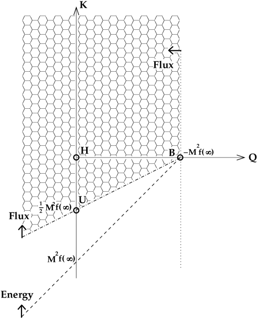
Figure 5: Weak Energy Condition and Quantum States

2.4.2 State-Independence and Boundary Conditions of the Basic Components

In the last Section I have demonstrated how different choices of the constants $K,Q$ lead to different expectations values of the EM tensor. I could show how particular values are related to specific boundary conditions that determine the local quantum state of the system. Thereby I have assumed that the basic components, being the input of the conservation equation, are independent of these boundary conditions and exhibit a sufficiently nice behaviour near the boundary of the manifold.

I have noted already in the last Section that $T^{\theta}{}_{\theta}$ must fall off at least like $r^{-3}$ (and $T$ like $r^{-2}$) so that $f(\infty)$ is a finite number. This can be traced back to the fact that the propagation of the particles (showing an $r^{-2}$ behaviour) occurs radially as I only consider s-waves. This manifests itself also by the free constants $K,Q$ which determine the radiational part of those components of the EM tensor that represent the physical degrees of freedom of the system.

The state-independence of the components $T^{\theta}{}_{\theta}$ and $T$ can be demonstrated by some simple physical considerations. If they were state-dependent the function $f$ (92) would be different in the $\left|U\right>$,$\left|H\right>$ and $\left|B\right>$-state and I would mark it then by a corresponding index $f_{U},f_{H},f_{B}$. In particular, its value at spatial infinity would depend on the choice of quantum state. The asymptotic energy density in the $\left|U\right>$ and $\left|H\right>$ state would become

$$T_{tt}\stackrel{{\scriptstyle r\to\infty}}{{\propto}}\left(-\frac{1}{2r^{2}}+O\left(r^{-3}\right)\right)\cdot\left\{\begin{array}[]{c}2f_{H}(\infty)\hskip 56.9055pt,\left|H\right>\\ 1f_{U}(\infty)\hskip 56.9055pt,\left|U\right>\end{array}\right..$$ (95)

In the static approximation the asymptotic energy density of the $\left|H\right>$-state is exactly twice the one in the $\left|U\right>$-state. This is due to the balancing incoming flux that doubles the number of particles with a certain energy in the asymptotic region. Thus I conclude that $f_{H}(\infty)=f_{U}(\infty)$ and, because $f$ is a linear combination of $T$ and $T^{\theta}{}_{\theta}$, it is likely that $\left<U\left|T\right|U\right>=\left<H\left|T\right|H\right>$ and $\left<U\left|T^{\theta}{}_{\theta}\right|U\right>=\left<H\left|T^{\theta}{}_{\theta}\right|H\right>$ on the whole spacetime (in fact the weaker result $f_{H}(\infty)=f_{U}(\infty)$ is at least sufficient to calculate the correct Hawking flux).

It is not possible to show the equivalence of the basic components in the Boulware state by similar physical arguments since the state itself exhibits unphysical properties. However, the essential difference to the other two states is that the asymptotic states (incoming and outgoing) are eliminated completely. The state-independence of the basic components just shows that they are independent of the asymptotic particle states but influenced only by the spacetime geometry. Thus, it holds for all states in which the total flux is negligible as compared to the spacetime curvature near the horizon:

$$\left<U\left|T\right|U\right>=\left<H\left|T\right|H\right>=\left<B\left|T\right|B\right>$$

$$\left<U\left|T^{\theta}{}_{\theta}\right|U\right>=\left<H\left|T^{\theta}{}_{\theta}\right|H\right>=\left<B\left|T^{\theta}{}_{\theta}\right|B\right>.$$ (96)

The state-independence of the basic components presumably breaks down when backreaction effects become important because then the scalar field contributes as much to the spacetime curvature as the BH.

3 The Effective Action

The effective action contains the whole information on a quantum system and is therefore the basis to compute expectation values of the physical observables. The classical scalar action (2) formally describes free particles as it does not contain a self-interaction term (e.g. $\lambda\cdot S^{4}$) or any interaction with other particles. In this thesis the gravitational metric field $g$ is treated as a classical field, hence it does not increase the order in $\hbar$ through interaction with $S$. The only possible Feynman graphs are isolated lines (corresponding to classical propagation) and single scalar loops (a line that is bent to a circle and connected at the ends). The dynamics of the system therefore is purely classical, the quantum theory enters only by the vacuum energy. The full interaction is thus described by a one-loop effective action and can be expressed by the functional determinant of the Laplace operator which determines the classical dynamics of the scalar field (I define the Laplace operator as the total quadratic term in the scalar action).

The main problem is that the classical EOM of a scalar field on a Schwarzschild spacetime cannot be solved exactly, i.e. the Green function cannot be given in a compact form. This means that the interaction of the scalar particle with the gravitational field needs to be solved perturbatively. The starting point of the perturbational analysis in my approach is the so-called heat kernel which essentially is the exponentiated Laplacian times a proper time. At this point one has to distinguish between massless and massive scalar particles.

Massless particles (or even very light particles) may cross very large distances during a finite period of proper time (measured in their rest frame). Their interaction with the gravitational field therefore cannot be considered as being local, merely they seem to interact with the whole manifold at once – the scalar loop, corresponding to a measurement of the EM tensor, is extremely large and extends over the whole spacetime. If the particle has a very small though finite mass $m$, the gravitational field, proportional to the BH mass $M$, slows down the particle and thereby reduces the size of the loop – one can say that the mass term $m^{2}S^{2}$ has the effect of a localising potential in the gravitational field. A particle can be considered as being localised if its mass times the BH mass is much larger than one: $mM\gg 1$. This condition determines the form of the effective action: if it is fulfilled, the effective action can be given in a local form and all expectation values measured at a certain spacetime point can be calculated from the geometry at this point. If the particle is too light, on a given BH spacetime, the effective action becomes a non-local expression that can be expressed as multiple integrals over the manifold.

In the case of massless particles the perturbation theory consists of counting the number of (non-local) interactions with the gravitational field. It is introduced by a formal separation of the spacetime metric into a flat background and a perturbing part representing the gravitational interaction. The result is a series of multiple integrals over the manifold where the integrand is a curvature term and a Green function which gives the probability of the particle to travel from the point of measurement to the point of interaction. Each integration corresponds to an interaction of the scalar particle with the gravitational field and increases the order in the curvature (the order in $\hbar$ is always $1$ as all interactions occur on a single loop). The convergence of the series thus depends on the strength of the curvature (as compared to the Planck curvature).

Figure 6: Non-local Interaction of Massless Particles

In Figure 5 I have represented the scalar particle by a smooth line and the gravitational field by jagged lines. $x$ is some fixed point of measurement, while each point of interaction is averaged over the whole manifold. The perturbation series converges, because the zeroth order vanishes (i.e. the flat spacetime value) and the main contribution comes from the first non-local order. The difficulty lies in finding the Green functions which are generally not given in a closed analytical form. The two-dimensional case is particular in this respect, because there one can find a local form of the effective action even in the massless case.

For sufficiently massive particles $m\gg\frac{1}{M}$ the loop is contracted to the point of measurement and the interaction can be considered as to happen at this single point. The effective action is then given by a local expansion, where by each order increases again the order in the curvature and simultaneously the order in the parameter $\alpha=\frac{1}{mM}$. The convergence condition then becomes $\alpha\ll 1$. The perturbation is performed by expanding the heat kernel for small values of the proper time, corresponding to small lengths of the scalar loop. For increasing parameter $\alpha$ the approximation to consider the measurement process as being local gets worse and contributions from larger proper times spoil the convergence of the series.

To deal with functional determinants of operators requires mathematical methods which are restricted to elliptic operators [25]. It is therefore necessary to Euclideanise the Lorentzian Laplace operator by the introduction of a Riemannian spacetime metric (I will speak of Euclideanisation, as it is common in particle physics, though a curved spacetime with Euclidean signature $(1,1,1,1)$ clearly has a Riemannian metric). This is realized by defining an imaginary time-variable $\tau=i\cdot t$ and multiplication of the whole metric by a factor $-1$, so that the complete transformation becomes $(1,-1,-1,-1)\to(1,1,1,1)$ (the overall minus sign is the greatest disadvantage of my sign-convention as one has to be particularly careful with signs when switching from the Lorentzian to the Riemannian spacetime). Accordingly the measure changes as $\sqrt{-g}\to\sqrt{g}$. The Lorentzian Laplace (d’Alembert) operator $\square$ is replaced by minus the Euclidean Laplace operator $\triangle$. For the transformation of the action see Appendix E (456). Whenever confusion is possible I mark Euclidean quantities by an index ${\cal E}$ and Lorentzian quantities by an index $\cal M$.

The effective action (36) is defined as a sum over all possible configurations of the scalar field on the background spacetime. In principle one could approximate numerically the eigenfunctions $\phi_{n}$ and eigenvalues $-\lambda_{n}$ of the Laplace operator $\triangle$ and calculate the effective action explicitly. For analytical calculations, however, the form (36) is rather inconvenient. As the eigenfunctions and eigenvalues are determined by the geometrical and topological (boundary terms) properties of the manifold one can describe the effective action in a purely geometrical and topological way. I start with formally integrating out the path integral by expanding the scalar field into eigenfunctions $S=\sum_{n}c_{n}\phi_{n}$:

$$W_{\cal E}[g]=-\ln\int{\cal D}S\cdot e^{-L^{\cal E}_{m}[g]}=-\ln\int{\cal D}S\cdot e^{\frac{1}{2}\int_{M}S\triangle S\sqrt{g}d^{4}x}\\ =-\ln\int\prod_{n}\left\{dc_{n}\cdot e^{-\frac{\lambda_{n}}{2}c^{2}_{n}}\right\}=-\ln\prod_{n}\sqrt{\frac{2\pi}{\lambda_{n}}}\\ =:\frac{1}{2}\ln\det(-\triangle)+\text{const.}=\frac{1}{2}\textrm{tr}\ln(-\triangle)+\text{const.}\,.$$ (97)

The integrations over the coefficients $c_{n}$ are simply Gaussian integrals

$$\int_{-\infty}^{\infty}e^{-\alpha x^{2}}dx=\sqrt{\frac{\pi}{\alpha}}.$$ (98)

In the exponent I have used the orthogonality condition of the eigenfunctions:

$$(\phi_{n},\phi_{m})=\int_{M}\phi_{n}\cdot\phi_{m}\sqrt{g}d^{4}x=\delta_{mn}.$$ (99)

The path integral measure has been derived by $||\delta S||^{2}=(\delta S,\delta S)=\sum_{n}(\delta c_{n})^{2}$ and hence ${\cal D}S=\prod_{n}dc_{n}$.

By equation (97) I have eliminated the scalar field from the effective action and reduced it to a purely geometrical expression. This simple relation holds for any (free) scalar field action that is quadratic in the fields. Hence I can generalise the Laplace operator by adding an endomorphism $E$ to the geometric Laplacian ${\cal O}=-\triangle 1\text{l}-E$. The sign is chosen such that the eigenvalues of ${\cal O}$ are positive. $E$ is defined as some bounded, linear map from the space of fields into itself. If I consider commuting scalar fields that do not possess inner degrees of freedom an endomorphism is simply given by the multiplication by some function. $1\text{l}$ denotes the identity endomorphism which in the case of scalar fields corresponds to a multiplication by $1$.

I mention another important point: by performing a partial integration in the first line of (97) I have dropped a boundary term

$$\frac{1}{2}\int_{M}g^{\rho\sigma}\nabla_{\rho}(S\nabla_{\sigma}S)\sqrt{-g}d^{4}x$$ (100)

by assuming natural boundary conditions (i.e. sufficiently rapidly vanishing fields). As discussed in Section 2.4 the boundary conditions are closely related to the quantum state of the effective action, and hence all expectation values derived from it. Natural boundary conditions generally imply that there are no occupied real particle states in the asymptotic region. This means that there is no incoming or outgoing flux which, according to the examinations of Section 2.4, corresponds to the Boulware state $\left|B\right>$. For the moment I will forget about the boundary conditions and concentrate on the local properties of the functional determinant. When considering expectation values it will turn out that general boundary conditions can be restored at the level of expectation values by use of the CF method.

The effective action associated to the Laplacian ${\cal O}$ is related to its eigenvalues, up to a constant that I discard in the following, by

$$W[g]=\frac{1}{2}\ln\det{\cal O}=\frac{1}{2}\ln\prod_{n}\lambda_{n}=\frac{1}{2}\textrm{tr}\left(\ln{\cal O}\right)=\frac{1}{2}\sum_{n}\ln\lambda_{n}.$$ (101)

Expression (101) in general is IR ($\ln 0$) and UV divergent ($\ln\infty$). To extract information from it I must therefore employ some regularisation. For the moment I postpone the IR problem by assuming that the particles are massive (this can be managed by adding an $m^{2}$-term to the endomorphism $E$).

3.1 Zeta-Function and Heat Kernel

With regard to the UV divergence I will use the “zeta-function regularisation”. This divergence appears if there are infinitely many large eigenvalues and (or) the eigenvalues increase without bound. In this regularisation every term in the sum of the $\ln\lambda_{n}$’s is multiplied by a factor $\lambda_{n}^{-s},s>0$. The contribution of large eigenvalues may then be neglected: $\lim_{\lambda\to\infty}\lambda^{-s}\ln\lambda=0$. The regularised effective action is given by

$$W[g,s]^{reg}=\frac{1}{2}\sum_{n}\lambda_{n}^{-s}\ln\lambda_{n}=-\frac{1}{2}\frac{d}{ds}\sum_{n}\lambda_{n}^{-s}.$$ (102)

The regularisation is removed by taking the limit $s\to 0$. By analogy to the Riemann zeta-function one introduces the zeta-function of the operator ${\cal O}$:

$$\zeta_{\cal O}[s]:=\sum_{n}\lambda_{n}^{-s}=\textrm{tr}\left({\cal O}^{-s}\right).$$ (103)

The effective action can then be written as

$$W[g]=-\frac{1}{2}\frac{d}{ds}\zeta_{\cal O}[s]\biggm{|}_{s=0}.$$ (104)

Now I bring the zeta-function into a form that is particularly appropriate for perturbational analysis. The $\Gamma$-function for complex arguments is defined as

$$\Gamma(s)=\int_{0}^{\infty}d\tau\tau^{s-1}e^{-\tau}.$$ (105)

A shift in the integration variable $\tau\to\lambda\tau$ leads to

$$\Gamma(s)=\lambda^{s}\int_{0}^{\infty}d\tau\tau^{s-1}e^{-\lambda\tau}.$$ (106)

Thus, the zeta-function can be written as

$$\zeta_{\cal O}[s]=\frac{1}{\Gamma(s)}\int_{0}^{\infty}d\tau\tau^{s-1}\sum_{n}e^{-\lambda_{n}\tau}=\frac{1}{\Gamma(s)}\int_{0}^{\infty}d\tau\tau^{s-1}\textrm{tr}\left(e^{-{\cal O}\tau}\right).$$ (107)

$e^{-{\cal O}\tau}$ is the so-called heat kernel of the operator ${\cal O}$. In a coordinate basis it reads:

$$G_{\cal O}(x,y;\tau)=\left<x\left|e^{-{\cal O}\tau}\right|y\right>=\sum_{n}\sum_{m}\left<x|n\right>\left<n|e^{-{\cal O}\tau}|m\right>\left<m|y\right>\\ =\sum_{n}\phi_{n}(x)\phi_{n}(y)e^{-\lambda_{n}\tau}.$$ (108)

The coordinate basis functions obey the orthonormality condition $\left<x|y\right>=\frac{1}{\sqrt{g}}\delta^{4}(x-y):=\delta^{4}(x,y)$. The heat kernel fulfils the heat equation

$$\left(\frac{\partial}{\partial\tau}+{\cal O}_{x}\right)G_{\cal O}(x,y;\tau)=0$$ (109)

with initial condition $G_{\cal O}(x,y;0)=\delta^{4}(x,y)$. It can be interpreted as the probability of a particle to be found at a spacetime point $y$ after a time $\tau$ has passed in its rest frame when starting from point $x$. The diagonal heat kernel $G_{\cal O}(x,x;\tau)$ describes the closed loop of a test particle in the measurement process. A mass term in the action leads to an $m^{2}$-term in the Laplacian and hence causes an exponential damping of big loops with large values of the proper time $\tau$. If it is sufficiently strong the heat kernel can be expanded into a local series for small values of $\tau$. For massless particles even infinite proper times $\tau$ contribute to the same order and the heat kernel inevitably produces non-localities.

The relation between the zeta-function and the heat kernel is given by

$$\zeta_{\cal O}[s]=\frac{1}{\Gamma(s)}\int_{0}^{\infty}d\tau\tau^{s-1}\int_{M}G_{\cal O}(x,x;\tau)\sqrt{g}d^{4}x.$$ (110)

3.1.1 Seeley-DeWitt Expansion

I start with discussing the local expansion of the heat kernel. Note that the methods of this Section can only be applied if a sufficient damping for large proper times $\tau$ is provided (see Section 3.1.3). On a $d$-dimensional manifold the diagonal heat kernel can be expanded around $\tau=0$ as [25]

$$G_{\cal O}(x,x;\tau)\stackrel{{\scriptstyle\tau\to 0}}{{=}}\frac{1}{(4\pi\tau)^{\frac{d}{2}}}\sum_{n=0}^{\infty}a_{n}(x,x)\tau^{\frac{n}{2}}.$$ (111)

The $a_{n}$ are called Seeley-DeWitt coefficients. The odd coefficients $a_{2n+1}$ are zero if the fields fulfil natural boundary conditions. From now on I assume that $a_{2n+1}=0$ for all $n$.

The coefficients with even index can be calculated from the heat equation (109). Following [2, 3] I make an ansatz for the heat kernel with different spacetime point arguments:

$$G_{\cal O}(x,y;\tau)=\frac{\sqrt{\Delta(x,y)}}{(4\pi\tau)^{\frac{d}{2}}}e^{-\frac{\sigma(x,y)}{2\tau}}\sum_{n=0}^{\infty}a_{2n}(x,y)\tau^{n}.$$ (112)

The bi-tensors $\sigma(x,y)$ (462) and $\Delta(x,y)$ (469) which appear in this expression are explained in Appendix F.2. $\sigma$ is related to the geodesic distance of two points and leads to an exponential damping for large point-separations. $\Delta$ is needed for coordinate invariance and becomes $1$ for $y=x$. First I show that the Ansatz (112) fulfils the initial condition:

$$\lim_{\tau\to 0}\int_{M}G_{\cal O}(x,y;\tau)\sqrt{g}d^{d}x\\ \approx\lim_{\tau\to 0}\frac{1}{(4\pi\tau)^{\frac{d}{2}}}\int_{-\infty}^{\infty}e^{-\frac{g_{00}(x^{0}-y^{0})^{2}+g_{11}(x^{1}-y^{1})^{2}+\dots}{4\tau}}\sqrt{g}dx^{0}dx^{1}\dots=1.$$ (113)

Thus $G_{\cal O}(x,y;\tau)$ becomes a delta-function for $\tau\to 0$. If we put (112) into (109) we obtain recurrence relations for the $a_{n}(x,y)$:

$$\left[-\frac{d}{2\tau}+\frac{\sigma}{2\tau^{2}}\right]\sum_{n}a_{2n}\tau^{n}+\sum_{n}n\,a_{2n}\tau^{n-1}\\ =\left[\frac{\triangle\sqrt{\Delta}}{\sqrt{\Delta}}-\left(\frac{\nabla\sqrt{\Delta}\nabla\sigma}{\sqrt{\Delta}}+\frac{\Delta\sigma}{2}\right)\frac{1}{\tau}+\frac{(\nabla\sigma)^{2}}{4\tau^{2}}\right]\sum_{n}a_{2n}\tau^{n}\\ +2\sum_{n}\frac{\nabla\sqrt{\Delta}\nabla a_{2n}}{\sqrt{\Delta}}\tau^{n}-\sum_{n}\nabla\sigma\nabla a_{2n}\tau^{n-1}+\sum_{n}(\triangle+E)a_{2n}\tau^{n}.$$ (114)

Using the identities $(\nabla\sigma)^{2}=2\sigma\,,\,D^{-1}\nabla_{\mu}(D\nabla^{\mu}\sigma)=d$ (464,468) this can be simplified to

$$\nabla\sigma\nabla a_{0} = 0$$ (115)

$$(n+2)a_{2n+2}+\nabla\sigma\nabla a_{2n+2} = \frac{\triangle(\sqrt{\Delta}a_{2n})}{\sqrt{\Delta}}+Ea_{2n},\,n>0.$$ (116)

By taking the coincidence limit $y\to x$ one can calculate the diagonal coefficients $a_{2n}(x,x)$. For this we need the coincidence limits of the involved bi-tensors and their derivatives:

         $\sigma\to 0$ $\sqrt{\Delta}\to 1$ $a_{0}\to 1$ $\sigma_{;\mu}\to 0$ $\sqrt{\Delta}_{;\mu}\to 0$ ${a_{0}}_{;\mu}\to 0$ $\sigma_{;\mu\nu}\to g_{\mu\nu}$ $\sqrt{\Delta}_{;\mu\nu}\to\frac{R_{\mu\nu}}{6}$ ${a_{0}}_{;\mu\nu}\to\frac{\Omega_{\mu\nu}}{2}$ $\sigma_{;\mu\nu\rho\sigma}\to-\frac{1}{3}(R_{\mu\nu\rho\sigma}+R_{\mu\sigma\rho\nu})$

                                                         Table 3
Some of these relations are derived in Appendix F.2. $\Omega_{\mu\nu}=-\Omega_{\mu\nu}$ is the gauge curvature associated to the gauge connection that might be present, see Appendix F.1 (460) – if there are no gauge degrees of freedom it vanishes. Starting from $a_{0}(x,x)=1$ I can calculate all higher diagonal Seeley-DeWitt coefficients. For instance, for $n=0$ I obtain the relation

$$a_{2}+\nabla\sigma\nabla a_{2}=\frac{\triangle\sqrt{\Delta}}{\sqrt{\Delta}}a_{0}+2\frac{\nabla\sqrt{\Delta}\nabla a_{0}}{\sqrt{\Delta}}+\triangle a_{0}+Ea_{0}$$ (117)

which in the coincidence limit yields $a_{2}=\frac{R}{6}1\text{l}+E$ (note that $g^{\mu\nu}\Omega_{\mu\nu}=0$). The first three Seeley-DeWitt coefficients are given by:

$a_{0}=1\text{l}$ $a_{2}=\frac{1}{6}(R1\text{l}+6E)$ $a_{4}=\frac{1}{360}[60\triangle E+60RE+180E^{2}+30\Omega_{mn}\Omega^{mn}$          $+(12\triangle R+5R^{2}-2R_{mn}R^{mn}+2R_{mnop}R^{mnop})1\text{l}]$ $a_{6}=\frac{1}{360}[6\triangle\triangle E+30E\triangle E+30(\triangle E)E+30E_{;m}E^{;m}+60E^{3}+12E\Omega_{mn}\Omega^{mn}$          $+6\Omega_{mn}E\Omega^{mn}+12\Omega_{mn}\Omega^{mn}E+10R\triangle E+4R_{mn}E^{;mn}+12R_{;m}E^{;m}$          $-6E_{;m}\Omega^{mn}{}_{;n}+6\Omega^{mn}{}_{;n}E_{;m}+30E^{2}R+12E\triangle R+5ER^{2}-2ER_{mn}R^{mn}$          $+2ER_{mnop}R^{mnop}]+\frac{1}{9\cdot 7!}[81R_{mnop,q}R^{mnop,q}+108R_{mnop}\triangle R^{mnop}$          $-44R_{mnop}R^{mn}{}_{qr}R^{opqr}-80R_{mnop}R^{m\,\,o}_{\,\,\,\,\,q\,\,r}R^{nqpr}$          $+42RR_{mnop}R^{mnop}-48R_{mn}R^{m}{}_{opq}R^{nopq}]1\text{l}+\dots$

                                                         Table 4
They are taken from [25] where $a_{6}$ is listed completely – here I have just quoted the terms I will need in this work. Note that all geometric objects like the Ricci tensor $R_{mn}$ belong to the Euclideanised manifold. For convenience I have written all tensors in vielbein components. Terms that differ only by the position of its elements, like $E\Omega_{mn}\Omega^{mn}$ and $\Omega_{mn}E\Omega^{mn}$, become identical if the fields commute.

3.1.2 General Form of the Zeta-Function

The zeta-function (103) of an operator ${\cal O}$ is related to the effective action of the corresponding quantum field (104). When calculating vacuum expectation values by taking functional derivatives of the effective action this relation may be modified by the appearance of new operators in $\zeta_{\cal O}[s]$. In this respect it proves useful to define a general zeta-function [25]

$$\zeta_{\cal O}[s;{\cal Q}]=\textrm{tr}_{L^{2}}({\cal Q\cdot O}^{-s})=\sum_{n}\lambda^{-s}_{n}\cdot\textrm{tr}(\pi(\lambda_{n};{\cal O}){\cal Q}),$$ (118)

where ${\cal Q}$ is some other operator. $\pi[\lambda_{n};{\cal O}]$ is the projection operator that projects onto the eigenspace of ${\cal O}$ belonging to the eigenvalue $\lambda_{n}$. By performing the same steps as before I can introduce the general heat kernel

$$G_{\cal O}(x,y;\tau)=\left<x\left|{\cal Q}e^{-{\cal O}\tau}\right|y\right>.$$ (119)

Again the diagonal heat kernel can be expanded around $\tau=0$:

$$G_{-\triangle}(x,x;\tau)=\frac{1}{(4\pi)^{\frac{d}{2}}}\sum_{n=0}^{\infty}a_{n}[{\cal Q;O}]\tau^{\frac{n-d}{2}}.$$ (120)

The original Seeley-DeWitt coefficients are given by the special case that ${\cal Q}$ is the identity endomorphism: $a_{n}=a_{n}[1\text{l};{\cal O}]$. The simplest case of a non-trivial general zeta-function is that ${\cal Q}$ is a function ${\cal Q}=f1\text{l},f\in C^{\infty}(M)$. The Seeley-DeWitt coefficients of the corresponding heat kernel expansion can then be obtained easily from the original ones (still ${\cal O}=-\triangle-E$). Defining an operator ${\cal O}^{\prime}=-\triangle-E-\varepsilon f$ yields the relation

$$\frac{d}{d\epsilon}\textrm{tr}\left[e^{(\triangle+E+\varepsilon f)\tau}\right]\biggm{|}_{\varepsilon=0}=\tau\cdot\textrm{tr}\left[fe^{(\triangle+E)\tau}\right].$$ (121)

If I insert the corresponding Seeley-DeWitt expansions into this relation I get a formula for the general coefficients

$$a_{n}[f;{\cal O}]=\frac{d}{d\varepsilon}a_{n+2}[{\cal O}^{\prime}]\biggm{|}_{\varepsilon=0},$$ (122)

where on the r.h.s. we have the original coefficient $a_{n+2}$ of the operator ${\cal O}^{\prime}$. Some general $a_{n}[f;{\cal O}]$ are collected in Table 5.

$a_{0}[f;{\cal O}]=f$ $a_{2}[f;{\cal O}]=\frac{1}{6}[Rf+\triangle f+6Ef]$ $a_{4}[f;{\cal O}]=[\frac{1}{60}\triangle\triangle f+\frac{1}{6}(E\triangle f+f\triangle E+E_{;m}f^{;m})+\frac{1}{2}E^{2}f+\frac{1}{6}EfR$                  $+\frac{5}{60}f\Omega_{mn}\Omega^{mn}+\frac{1}{72}(2R\triangle f+fR^{2})+\frac{1}{90}R_{mn}f^{;mn}$                  $+\frac{1}{30}(R_{;m}f^{;m}+f\triangle R)-\frac{1}{180}fR_{mn}R^{mn}+\frac{1}{180}fR_{mnop}R^{mnop}]$

                                                         Table 5

3.1.3 Application of the Asymptotic Expansion

In the following I specify for a four-dimensional spacetime. The same arguments apply in the two-dimensional case. There are two important cases when the asymptotic heat kernel expansion can be applied successfully. First, I can calculate the trace anomaly in arbitrary even dimensions directly by $\zeta[0]$ which is always a finite expression, see Appendix C.2. As it only consists of a finite number of terms I need not worry about convergence conditions. Second, if there exists a sufficiently strong damping for big values of the proper time $\tau$ the Seeley-DeWitt expansion converges and I can calculate the effective action. Note that the latter always contains UV divergent terms that must be renormalised – the convergence of the series only guarantees IR finiteness.

In the classical Euclidean action a damping term by definition has the form

$$L^{\cal E}_{D}=\int_{M}\frac{SDS}{2}\sqrt{g}d^{4}x.$$ (123)

$D$ might be a constant like $m^{2}$ or an arbitrary analytical function. Such a term modifies the Laplacian as ${\cal O}\to{\cal O}+D$. I can pull the damping term out of the modified heat kernel, whereby commutator terms with the original Laplacian have to be taken into account:

$$G_{\cal O}(x,y;\tau)=e^{-D\tau}\left<x\left|\left(1+\frac{\tau^{2}}{2}[D,{\cal O}]+O(\tau^{3})\right)e^{{\cal O}\tau}\right|y\right>.$$ (124)

The commutators can be lifted back into the heat kernel to the right, thereby producing new Laplacians ${\cal O}_{n}$ with new endomorphisms$E_{n}$:

$$G_{\cal O}(x,y;\tau)=e^{-D\tau}\left<x\left|e^{{\cal O}\tau}+c_{1}\,e^{{\cal O}_{1}\tau}\tau+c_{2}\,e^{{\cal O}_{2}\tau}\tau^{2}+O(\tau^{3})\right|y\right>.$$ (125)

$c_{1},c_{2}\dots$ are constants. Now I insert the Seeley-DeWitt expansions of the new heat kernels. Clearly, the Seeley-DeWitt coefficients depend on the endomorphisms, being different for each term in general. The zeta-function is then given by an infinite sum of integrals of the type

$$\int_{0}^{\infty}\tau^{s+k}e^{-D\tau}=\Gamma[1+s+k]\frac{1}{D^{(1+s+k)}},$$ (126)

where $k$ goes from $-3$ to $+\infty$:

$$\zeta_{\cal O}[s]=\frac{1}{(4\pi)^{2}\Gamma[s]}\int_{M}\left\{\Gamma[s-2]D^{2-s}a_{0}^{(0)}+\Gamma[s-1]D^{1-s}(a_{2}^{(0)}+c_{1}a_{0}^{(1)})\right.\\ \left.+\Gamma[s]D^{-s}(a_{4}^{(0)}+c_{1}a_{2}^{(1)}+c_{2}a_{0}^{(2)})+\cdots\right\}\sqrt{g}d^{4}x.$$ (127)

$a_{n}^{(i)}$ are the coefficients belonging to ${\cal O}_{i}$, ${\cal O}_{0}={\cal O}$. One can see immediately that $\zeta[0]$ is always finite if $D$ is a regular function. Namely, because of $\Gamma[s]^{-1}=s+O(s^{2})$ only the first three terms contribute. There is no IR problem for large values of $\tau$.

To the effective action contribute all terms in the series as it is obtained by differentiation for $s$. Therefore, I must investigate the convergence of the whole series, the basic assumption being that $a_{2n+2}<a_{2n}$. There are three different cases:

• If all commutators vanish (which is true if $[D,{\cal O}]=0$) one gets the original series with coefficients $a_{2n}$. A necessary condition is that $a_{2n+4}/D^{n}$ is finite at all spacetime points $x\in M$ for all $n$. The series converges if $\lim_{n\to\infty}\text{sup}_{x\in M}(a_{2n+2}/Da_{2n})<1$.

• If there is a finite number of nonvanishing commutators, one has to consider the convergence criterion for all series separately, where it is to be expected that the highest series (corresponding to ${\cal O}_{max}$) is the most problematic.

• If there are infinitely many commutators the condition $D>1$ must be fulfilled.

3.2 Covariant Perturbation Theory

In this Section I present a short introduction to the covariant perturbation theory developed by Barvinsky and Vilkovisky [4, 26]. I will only give a guideline how to construct the non-local effective action, starting from the heat kernel, and demonstrate this for the simplest case. The formalism only works in even dimensions, hence I introduce the notation $d=2\omega,\omega=1,2,\dots$.

The Seeley-DeWitt expansion cannot be applied to massless particles in the general case. As I have shown in the last Section, the local perturbation series diverges if the damping factor $D$ (e.g. the squared mass of the particle) goes to zero. In the absence of any self-interaction that “localises” the particle in some finite spacetime volume the scalar particle can travel large spacetime regions within a small period of proper time. Hence the effective action, containing the information on the quantum mechanical expectation values, is supposed to consist of non-local terms in the form of multiple integrals over the whole manifold.

The appropriate formalism to derive this non-local effective action directly is the covariant perturbation theory. Just like the Seeley-DeWitt expansion it is based on the heat kernel, thus all quantities considered in this Section are Euclidean (or, more precisely, Riemannian). As already mentioned, the perturbational treatment is necessary because the classical EOM of the scalar field cannot be solved exactly. Like in QFT, the order of the perturbation counts the number of interactions, thereby increasing the order in the curvature. Note that the number of loops remains constantly $1$ as the gravitational field is considered as a classical field whose interaction is described by external lines that cling to the scalar loop (see Figure 5 at the beginning of this Chapter). If Quantum Gravity would play a role (e.g. by the exchange of virtual gravitons) an internal graviton line would increase the loop order by one, see Figure 3 in Section 1.2.1.

One begins by formally considering the gravitational field of the BH as some small perturbation of flat spacetime. Accordingly, the expectation value of the EM tensor in flat spacetime is the zeroth order of the perturbation theory. It is obvious that the first perturbative order cannot be small as compared to the zeroth order, but as the latter is renormalised to zero (in the vacuum state) the first order is the effective starting point of the series. The metric is divided into two terms

$$g_{\mu\nu}=\tilde{g}_{\mu\nu}+h_{\mu\nu},$$ (128)

where the metric $\tilde{g}$ represents the zeroth order. Its associated Riemann tensor thus shall vanish:

$$R^{\mu}{}_{\nu\rho\sigma}[\tilde{g}]=0.$$ (129)

Hence $\tilde{g}$ is in fact the metric of a flat Euclidean space and in a Cartesian coordinate system it becomes the flat metric $\delta$. The split of the metric into a “background part” $\tilde{g}$ and a perturbing part $h$ seems to contradict the covariance of this approach. However, this is just an intermediate step in the development of the perturbation series. The final form of the latter turns out to be (at each order) a covariant expression in the geometric objects describing the original manifold, depending solely on $g$. The physical picture is that the scalar particle is scattered zero, one, two etc. times on the full manifold (which in fact is a covariant object), whereas e.g. in the case of linearised gravity waves the manifold is indeed split into a background part $\tilde{g}$ and the part describing the propagating gravitational waves $h$ and hence this separation is manifest.

The effective action of Barvinsky and Vilkovisky covers the most general case, where the Laplacian acting on the scalar field consists of a geometric Laplacian, including a “gauge part”, and an endomorphism. With gauge part I mean the term of the connection that is added to the Levi-Civitá connection and is associated to some external gauge transformation applied to the scalar field. Barvinsky and Vilkovisky use the notation

$$\nabla_{\mu}S=\tilde{\nabla}_{\mu}S+\tilde{\Gamma}_{\mu}S.$$ (130)

$\tilde{\nabla}$ is the derivative operator associated to the metric $\tilde{g}$ – it becomes a partial derivative $\partial$ in a Cartesian coordinate system. $\tilde{\Gamma}$ meanwhile denotes the “rest” of the connection and hence must include the missing Christoffels of the full metric $g$ as well as the gauge part. In the general case the connection $\nabla$ produces both a geometric curvature $R^{\mu}{}_{\nu\rho\sigma}$ and a gauge curvature ${\cal R}_{\mu\nu}$ (in my notation the gauge curvature was $\Omega_{\mu\nu}$, see Appendix F.1 (460)). In this work I will only have to deal with the case ${\cal R}_{\mu\nu}=0$.

On the whole we have three types of curvatures contributing to the same order in the perturbation series (as can be seen from their equal dimensions), namely the geometric and gauge curvature, and the endomorphism that Barvinsky and Vilkovisky name $\tilde{P}$. It is related to the one used by me by $E=\tilde{P}-\frac{R}{6}$; his notation is especially convenient for the conformally coupled case in $4d$ where $\tilde{P}=0$.

By expanding the “curvatures” in $g$ around $\tilde{g}$, one obtains relations between $h$ and $\tilde{\Gamma}$ and these curvatures, e.g. (see (381))

$$R^{\mu\nu\rho\sigma}[\tilde{g}+h]=R^{\mu\nu\rho\sigma}[g]+O(h)\\ =0+\frac{1}{2}\left(\tilde{\nabla}^{\rho}\tilde{\nabla}^{\mu}h^{\nu\sigma}-\tilde{\nabla}^{\rho}\tilde{\nabla}^{\nu}h^{\mu\sigma}-\tilde{\nabla}^{\sigma}\tilde{\nabla}^{\mu}h^{\nu\rho}+\tilde{\nabla}^{\sigma}\tilde{\nabla}^{\nu}h^{\mu\rho}\right)+O(h^{2}).$$ (131)

Vice versa one can consider this relation as expressing the perturbative metric $h$ in terms of the Riemann tensor $R^{\mu}{}_{\nu\rho\sigma}$ to the first perturbative order. By means of the Bianchi identity one can integrate this relation and in a convenient gauge one obtains (I will specify the meaning of such non-local expressions like $\triangle^{-1}$ as soon as I use them)

$$h^{\mu\nu}=2\frac{\delta^{\mu\nu}_{\rho\sigma}}{\triangle}R^{\rho\sigma}[g]+O(R^{2}).$$ (132)

An analogous relation can be obtained for the perturbative connection $\tilde{\Gamma}$ (where on the r.h.s. appear ${\cal R}_{\mu\nu}$ and $\tilde{P}$). These expressions only contain geometric objects depending on the metric $g$ of the full manifold. Furthermore, Barvinsky and Vilkovisky show that the full Laplacian (in this gauge) can be decomposed as

$$\triangle+E=g^{\mu\nu}\nabla_{\mu}\nabla_{\nu}=\triangle_{0}+h^{\mu\nu}\tilde{\nabla}_{\mu}\tilde{\nabla}_{\nu}+2(\tilde{g}^{\mu\nu}+h^{\mu\nu})\tilde{\Gamma}_{\mu}\tilde{\nabla}_{\nu}.$$ (133)

Note that the endomorphism $E$ has been absorbed in the gauge part of the connection (in the next Sections I will make use of this trick to shift terms between connection and endomorphism). $\triangle_{0}$ is simply the flat Laplacian for a particle with no gauge group acting on it.

The perturbation of the effective action emerges expanding the heat kernel by the decomposition of the Laplacian (133) and inserting (132). Then one can write the heat kernel as a sum of terms with increasing orders in the curvature factors

$$G_{\cal O}(\tau)=e^{-{\cal O}\tau}=\sum_{n=0}^{\infty}G^{n}_{\cal O}(\tau),$$ (134)

where $G^{n}_{\cal O}(\tau)$ has a power $n$ in the curvatures. As an illustration I will only consider the simplest case, where I have an endomorphism $E$ but no curvature neither gauge curvature, i.e. ${\cal O}=-\triangle_{0}-E$. In this case the perturbation of the heat kernel has the form

$$G^{0}_{\cal O}(\tau) = e^{\triangle_{0}\tau}$$ (135)

$$G^{n}_{\cal O}(\tau) = e^{\triangle_{0}\tau}\int_{0}^{\tau}e^{-\triangle_{0}\upsilon}E\cdot G^{n-1}_{\cal O}(\upsilon)d\upsilon,\,n\geq 1.$$ (136)

In a coordinate basis $G^{0}_{\cal O}(\tau)$ reads (112)

$$G^{0}_{\cal O}(x,y;\tau)=\frac{\sqrt{\Delta(x,y)}}{(4\pi\tau)^{\omega}}e^{-\frac{\sigma(x,y)}{2\tau}}a_{0}(x,y).$$ (137)

Note that $\sqrt{\Delta(x,y)}$, though defined via the metric $\tilde{g}$ of a flat space, only becomes $1$ in a Cartesian coordinate system. $a_{0}(x,y)$ is the parallel displacement operator (bi-unit) if acting on a scalar field, see Appendix F.2 (471). All other Seeley-DeWitt coefficients are zero due to the flatness of the space described by $\tilde{g}$. To construct the effective action I will need the trace of the heat kernel:

$$\text{tr}G^{0}_{\cal O}(\tau)=\int_{M}G^{0}_{\cal O}(x,x;\tau)\sqrt{g}d^{2\omega}x=\frac{1}{(4\pi\tau)^{\omega}}\int_{M}a_{0}(x,x)\sqrt{g}d^{2\omega}x.$$ (138)

This integral is divergent if the manifold has infinite size ($a_{0}(x,x)=1$ for scalar fields without external degrees of freedom). It produces the zero-point energy of the quantised EM tensor on a flat spacetime which is renormalised to zero – if some small finite value would remain after renormalisation (a cosmological constant) we would have a non-vanishing zeroth order and the general covariance would be broken (a background radiation selects out a preferred reference system). The term of first order in the curvature is still local:

$$\text{tr}G^{1}_{\cal O}(\tau)\\ =\int^{x}_{M}\int^{z}_{M}\int^{z^{\prime}}_{M}\left<x\right|e^{\triangle\tau}\left|z\right>\int_{0}^{\tau}\left<z\right|e^{-\triangle\upsilon}\left|z^{\prime}\right>E(z^{\prime})\left<z^{\prime}\right|e^{\triangle\upsilon}\left|x\right>d\upsilon\sqrt{g}d^{2\omega}x\cdots\\ =\int^{x}_{M}\int^{z}_{M}\int^{z^{\prime}}_{M}\left<x\right|e^{\triangle\tau}\left|z\right>E(z)\int_{0}^{\tau}\left<z\right|e^{-\triangle\upsilon}\left|z^{\prime}\right>\left<z^{\prime}\right|e^{\triangle\upsilon}\left|x\right>d\upsilon\sqrt{g}d^{2\omega}x\cdots\\ =\int_{M}\left<x\right|e^{\triangle\tau}\left|x\right>E(x)\tau\sqrt{g}d^{2\omega}x=\frac{\tau}{(4\pi\tau)^{\omega}}\int_{M}E(x)\sqrt{g}d^{2\omega}x.$$ (139)

In two dimensions ($\omega=1$) this local term is IR divergent, in higher dimensions UV divergent. In any case it may contribute to expectation values and must be regularised. Next I consider the term of second order in the curvature:

$$\text{tr}G^{2}_{\cal O}(\tau)\\ =\int^{x}_{M}\int^{z}_{M}\int_{0}^{\tau}\left<x\right|e^{\triangle(\tau-\upsilon)}\left|z\right>E(z)\upsilon\left<z\right|e^{\triangle\upsilon}\left|x\right>E(x)d\upsilon\sqrt{g}d^{2\omega}x\sqrt{g}d^{2\omega}z\\ =\int^{x}_{M}\int^{z}_{M}\int_{0}^{\tau}\upsilon\frac{\Delta(x,z)}{(4\pi\tau)^{\omega}}\left(\frac{\tau}{4\pi(\tau-\upsilon)\upsilon}\right)^{\omega}e^{-\frac{\sigma(x,z)\tau}{2(\tau-\upsilon)\upsilon}}\\ \cdot a_{0}(x,z)E(z)a_{0}(z,x)E(x)d\upsilon\sqrt{g}d^{2\omega}x\sqrt{g}d^{2\omega}z\\ =\frac{1}{(4\pi\tau)^{\omega}}\int^{x}_{M}\int_{0}^{\tau}\upsilon E(x)G^{0}_{\cal O}\left(x,x;\frac{(\tau-\upsilon)\upsilon}{\tau}\right)E(x)d\upsilon\sqrt{g}d^{2\omega}x\\ =\frac{1}{(4\pi\tau)^{\omega}}\int^{x}_{M}E(x)\int_{0}^{\tau}\upsilon\cdot e^{\triangle\frac{(\tau-\upsilon)\upsilon}{\tau}}d\upsilon E(x)\sqrt{g}d^{2\omega}x\\ =\frac{\tau^{2}}{(4\pi\tau)^{\omega}}\int^{x}_{M}E(x)\int_{0}^{1}a\cdot e^{\triangle a(1-a)\tau}daE(x)\sqrt{g}d^{2\omega}x\\ =\frac{\tau^{2}}{(4\pi\tau)^{\omega}}\int^{x}_{M}E(x)\int_{0}^{1}(1-a)e^{\triangle a(1-a)\tau}daE(x)\sqrt{g}d^{2\omega}x\\ =\frac{\tau^{2}}{(4\pi\tau)^{\omega}}\int^{x}_{M}E(x)\int_{0}^{1}\frac{e^{\triangle a(1-a)\tau}}{2}daE(x)\sqrt{g}d^{2\omega}x\\ :=\frac{\tau^{2}}{(4\pi\tau)^{\omega}}\int^{x}_{M}E(x)\frac{f(-\triangle\tau)}{2}E(x)\sqrt{g}d^{2\omega}x,$$ (140)

where I have defined the function

$$f(x)=\int_{0}^{1}e^{-a(1-a)x}da.$$ (141)

This function produces the non-localities in the second order of the covariant perturbation theory (as will be seen when doing explicit calculations).

The geometric curvature and the gauge curvature can be treated in the same way as the endomorphism by using the decomposition (133) of the full Laplacian. I will restrict myself to the second order of the perturbation theory, although in principle all orders are accessible by this formalism. In [26], Equation 2.1, the most general form of the trace of the heat kernel in general dimensions to the second order is given. Note that the Riemann tensor does not appear because it has been eliminated by the Bianchi identities. I adapt this formula according to my purpose, namely to study Hawking radiation of massless scalar fields from Schwarzschild BHs in the quasi-static phase:

• I substitute the endomorphism by $E=\tilde{P}-\frac{R}{6}$ because I consider minimally coupled scalars (in the $4d$ action).

• The scalar fields shall commute, hence I can drop the gauge curvature by setting ${\cal R}_{\mu\nu}=0$.

• The BH spacetime is almost perfectly a vacuum spacetime in the quasi-static phase, thus I can eliminate the Ricci tensor by the vacuum Einstein equations $R_{\mu\nu}=\frac{g_{\mu\nu}}{2}R$.

The trace of the heat kernel up to the second order of the non-covariant perturbation theory in even dimensions $d=2\omega$ then reads

$$\text{tr}\,e^{-{\cal O}\tau}=\frac{1}{(4\pi\tau)^{\omega}}\int_{M}\text{tr}\biggm{\{}1\text{l}+\tau\left(\frac{R}{6}+E\right)\\ +\tau^{2}\biggm{[}R\left(\frac{1}{16(-\triangle\tau)}+\frac{f(-\triangle\tau)}{32}+\frac{f(-\triangle\tau)-1}{8(-\triangle\tau)}+\frac{3[f(-\triangle\tau)-1]}{8(\triangle\tau)^{2}}\right)R\\ +E\left(\frac{f(-\triangle\tau)}{6}+\frac{f(-\triangle\tau)-1}{2(-\triangle\tau)}\right)R+R\frac{f(-\triangle\tau)}{12}E+E\frac{f(-\triangle\tau)}{2}E\biggm{]}\biggm{\}}\sqrt{g}d^{2\omega}x.$$ (142)

It is now manifest that the perturbation theory is indeed covariant which means that it only depends on tensorial objects of the full manifold described by $g$. The crucial point is that all geometric objects are in fact associated to the perturbing part of the metric $h$, but as the starting point of the series is a flat spacetime (given by $\tilde{g}$) one can replace (to the linear order) all objects by those associated to $g=\tilde{g}+h$. What remains is the zeroth order contribution (in (142) represented by the unity term $1\text{l}$). But as the latter does not contribute to the expectation values (apart from a renormalisation constant related to the cosmological constant which is here assumed to be zero) it does not spoil the general covariance.

The non-local form of the trace of the heat kernel can be regarded as the more comprising case – in the limit of sufficiently strong damping the Seeley-DeWitt expansion is recovered (it is neither difficult nor illuminating to show this explicitly, hence I refer to the papers of Barvinsky and Vilkovisky [4, 26]).

Finally, I will mention some points discussed by Barvinsky and Vilkovisky that will be important for this work. First they state that the conformally coupled scalar field in two dimensions (where $E=0$) is the only case where the covariant perturbation theory is applicable in $2d$.

I do not agree to this point and demonstrate in Chapter 5 that a non-local effective action (derived from the trace of the heat kernel) can be established in all cases and for all endomorphisms and metrics if an IR regularisation is introduced.

Barvinsky and Vilkovisky argue that the non-local form of the heat kernel allows to recover all boundary conditions of Lorentzian manifolds (which are not directly accessible in the Euclidean formalism) by simply representing the non-local terms as integrals over Green functions, thereby choosing the appropriate Lorentzian Green functions. Further, they state that expectation values in the common sense, the initial and final state both being in-states, are obtained by the use of the retarded Green function; the Feynman Green function merely leads to scattering probabilities from in- to out-states. With regard to these ideas I investigate the role of the Green functions by the Green function perturbation series in Section 5.4. Thereby I will come to the conclusion that the effective action is independent of the choice of the Green function in the static approximation. The quantum state merely seems to be determined by the spacetime geometry alone and in the Schwarzschild approximation it can be identified with the Boulware state $\left|B\right>$.

The way Barvinsky and Vilkovisky derive their effective action from the heat kernel differs from mine, see (104). This fact is not related to any of the considerations above, but it has some relevance for the renormalisation.

4 Hawking Radiation of Massive Scalars

The contribution of massive particles to the Hawking flux is assumed to be much smaller than that of massless particles if the BH is in the quasi-static phase. The BH temperature is then much lower than the rest mass of all elementary particles (except possibly neutrinos!) and the probability that massive particles are produced is therefore very small as compared to massless particles. The physical picture is that particle-antiparticle states of heavy particles self-interact on smaller distances and within smaller periods of time and thus decrease the probability that the BH catches the constituent with negative energy before pair-annihilation occurs. With decreasing BH mass, and hence increasing surface temperature, the particle production rate becomes more and more mass-independent.

In any case, there exists a lower limit for what I call “massive particles” imposed by the convergence condition of the Seeley-DeWitt expansion. It will turn out that this limiting value depends on the inverse of the BH mass which means that the strength of surface gravity determines if a particle is heavy enough as to be considered as massive. In this Chapter I will only treat massive particles in this sense, lighter particles are object of the non-local formalism developed for the massless case. The great advantage of (sufficiently) massive particles is that one can establish a local covariant perturbation series of the effective action via the Seeley-DeWitt expansion. The particle dynamics enters only by the perturbational expansion of the Euclidean Feynman Green function. This means that it is not necessary to know explicitly the Green functions of the massive scalar particles to compute the expectation values. Hence, the effective action is directly available for all even spacetime dimensions (for massless particles the two-dimensional case is somewhat particular because only there one can still find a local form of the effective action).

According to the above considerations, the effective action is given in a particular quantum state (namely the Boulware state) which is not suitable for the calculation of Hawking radiation. Therefore, I will only use it to compute the basic components which have been shown to be state-independent (see Section 2.4.2). The remaining components are then calculated by the conservation equation a la CF.

The advantage of massive particles is that one can work directly in four spacetime dimensions and avoids the additional difficulties and uncertainties of the dilaton model. Besides, one can still go over to two dimensions and compare the results of the dilaton model with the “correct” results of the $4d$-theory. This provides a check of the dilaton model at the quantum level that may give hints for the treatment of massless particles.

4.1 $4d$ Theory

The procedure in four dimensions is quite straightforward. I establish an effective action, whereby the mass-term guarantees IR regularity. Then I compute the basic components by variation for the metric to the first order of the perturbation theory; this part of the calculation is the most tedious one. Finally, I complete the EM tensor by the CF method and calculate the Hawking-flux in the vacuum state.

4.1.1 Effective Action

I consider the action (2) of a massive particle without internal degrees of freedom and without (further) self-interaction. The Euclidean Laplacian thus is given by $-\triangle+m^{2}$ (note that the mass term is invariant under Euclideanisation). To cover also the general case I add an (Euclidean) endomorphism $E$ to the Laplacian ${\cal O}+m^{2}=-\triangle-E+m^{2}$. ${\cal O}$ is the Laplacian of a massless scalar field with an arbitrary endomorphism. The corresponding heat kernel is given by

$$e^{(-{\cal O}-m^{2})\tau}=e^{-{\cal O}\tau}\cdot e^{-m^{2}\tau}.$$ (143)

The mass-term can be separated without producing further terms because it commutes with the remaining Laplacian. In the following I will assume that the mass-term provides a sufficient damping such that the heat kernel of ${\cal O}$ can be expanded in a Seeley-DeWitt series (111). The zeta-function of the full Laplacian then reads (107):

$$\zeta_{{\cal O}+m^{2}}[s]=\frac{1}{\Gamma(s)}\int_{0}^{\infty}d\tau\tau^{s-1}\int_{M}G_{{\cal O}+m^{2}}(x,x;\tau)\sqrt{g}d^{4}x\\ =\frac{1}{\Gamma(s)}\int_{0}^{\infty}d\tau\tau^{s-1}\int_{M}\left<x\left|e^{(-{\cal O}-m^{2})\tau}\right|x\right>\sqrt{g}d^{4}x\\ =\frac{1}{\Gamma(s)}\int_{0}^{\infty}d\tau\tau^{s-1}e^{-m^{2}\tau}\int_{M}G_{\cal O}(x,x;\tau)\sqrt{g}d^{4}x\\ =\frac{1}{\Gamma(s)}\int_{0}^{\infty}d\tau\tau^{s-1}\frac{e^{-m^{2}\tau}}{(4\pi\tau)^{2}}\int_{M}\sum_{n=0}^{\infty}a_{2n}\tau^{n}\sqrt{g}d^{4}x\\ =\frac{1}{(4\pi)^{2}\Gamma(s)}\int_{0}^{\infty}d\tau e^{-m^{2}\tau}\int_{M}\Bigm{[}\tau^{s-3}a_{0}+\tau^{s-2}a_{2}+\tau^{s-1}a_{4}+\tau^{s}a_{6}+\dots\Bigm{]}\sqrt{g}d^{4}x.$$ (144)

Note that the $\tau$-integrations are divergent in the limit $m\to 0$. The integrals over the proper time $\tau$ are simply representations of the Gamma-function. Thus I can formally write:

$$\zeta_{{\cal O}+m^{2}}[s]=\frac{1}{(4\pi)^{2}}\int_{M}\frac{1}{\Gamma(s)}\Bigm{[}\Gamma[s-2](m^{2})^{2-s}a_{0}+\Gamma[s-1](m^{2})^{1-s}a_{2}\\ +\Gamma[s](m^{2})^{-s}a_{4}+\frac{a_{6}}{m^{2}}+\frac{a_{8}}{m^{4}}+\dots\Bigm{]}\sqrt{g}d^{4}x.$$ (145)

The Gamma-functions have poles of first order at $s=0$ and at all negative integer values of $s$. By expanding them around $s=0$ I get

$$\Gamma[s-2] = \frac{1}{2s}+\left(\frac{3}{4}-\frac{\gamma_{E}}{2}\right)+O(s)^{1}$$ (146)

$$\Gamma[s-1] = -\frac{1}{s}+(\gamma_{E}-1)+O(s)^{1}$$ (147)

$$\Gamma[s] = \frac{1}{s}-\gamma_{E}+O(s)^{1}$$ (148)

$$\frac{1}{\Gamma(s)} = s+s^{2}\cdot\gamma_{E}+O(s)^{3}$$ (149)

$$\left(m^{2}\right)^{(k-s)} = \left(m^{2}\right)^{k}-s\cdot\left(m^{2}\right)^{k}\ln\left(m^{2}\right)+O(s),$$ (150)

where $\gamma_{E}$ is the Euler-Mascheroni constant. Plugging this into the zeta-function gives

$$\zeta_{{\cal O}+m^{2}}[s]\\ =\frac{1}{(4\pi)^{2}}\int_{M}\biggm{\{}\frac{a_{0}m^{4}}{2}\left[1+s\left(3/4-\ln m^{2}\right)\right]-a_{2}m^{2}\left[1+s\left(1-\ln m^{2}\right)\right]\\ +[1-s\ln m^{2}]a_{4}+s\left(\frac{a_{6}}{m^{2}}+\frac{a_{8}}{m^{4}}+\frac{2!a_{10}}{m^{6}}\right)+\dots+O(s)^{2}\biggm{\}}\sqrt{g}d^{4}x.$$ (151)

The Euclidean effective action according to (104) is obtained by differentiation for $s$ and then setting $s=0$:

$$W[g,m^{2}]=-\frac{1}{32\pi^{2}}\int_{M}\biggm{[}\frac{a_{0}m^{4}}{8}(3-2\ln m^{2})+a_{2}m^{2}(\ln m^{2}-1)-a_{4}\ln m^{2}\\ +\frac{a_{6}}{m^{2}}+\frac{a_{8}}{m^{4}}+\frac{2!a_{10}}{m^{6}}+\dots\biggm{]}\sqrt{g}d^{4}x.$$ (152)

For $m\to\infty$ the terms in the first line diverge, while the remaining terms tend to zero. In the last line of (144) one can see that these terms further exhibit bad UV behaviour, namely their $\tau$-integrals have poles at $\tau=0$. The first (divergent) terms in the Seeley-DeWitt expansion are connected to the renormalisation of the vacuum energy and gravitational radiation. The first coefficient $a_{0}$, which is simply constant, has to be removed to obtain zero vacuum energy in flat spacetime. In other words, the vacuum energy density in curved spacetime is renormalised by substracting the flat spacetime value which is assumed to be zero. The coefficients $a_{2},a_{4}$ cannot be interpreted this simply. $a_{2}$, as it only contains the scalar curvature, does not contribute to the EM tensor on a vacuum spacetime because there $R=0,R_{\mu\nu}=0$ (if the backreaction is neglected). Hence only $a_{4}$ causes problems. The factor $\ln m^{2}$ leads to diverging vacuum energy density for infinitely heavy particles, though it is expected that such particles do not contribute at all (at least in the stationary phase). After gravitational radiation has been renormalised a term $\propto a_{4}$ may still appear in the effective action (I come back to this point in Section 4.3). For the moment, and following [3], I drop these coefficients and define the renormalised Euclidean effective action as

$$W_{ren}[g,m^{2}]:=-\frac{1}{32\pi^{2}}\int_{M}\biggm{[}\frac{a_{6}}{m^{2}}+\frac{a_{8}}{m^{4}}+\frac{2!a_{10}}{m^{6}}+\dots\biggm{]}\sqrt{g}d^{4}x.$$ (153)

The Lorentzian effective action is related to the Euclidean one by $W_{\cal M}=iW_{\cal E}$, see Appendix E. If each term in the action is switched back by its own I must add a minus sign: $W_{\cal M}=-iW_{\cal E}$!. The Euclidean time-coordinate transforms as $d\tau=idt$. Further, one has to replace the geometric objects in the Seeley-DeWitt coefficients according to the rules given in Appendix E. The renormalised Lorentzian effective action reads

$$W^{ren}_{\cal M}[g,m^{2}]:=-\frac{1}{32\pi^{2}}\int_{M}\biggm{[}\frac{a_{6}^{\cal M}}{m^{2}}+\frac{a_{8}^{\cal M}}{m^{4}}+\frac{2!a_{10}^{\cal M}}{m^{6}}+\dots\biggm{]}\sqrt{-g}d^{4}x_{\cal M}.$$ (154)

In the following I will omit the index ${\cal M}$ as long as I work with the Lorentzian effective action.

Until now I have assumed that the damping provided by the mass term is sufficient to guarantee the convergence of the Seeley-DeWitt expansion (otherwise I cannot apply it). Now I will examine when this is indeed the case. According to the considerations in Section 3.1.3 the whole series converges if $\lim_{n\to\infty}\text{sup}_{x\in M}(a_{2n+2}/m^{2}a_{2n})<1$. Because I only know the first coefficients explicitly I can only make a crude estimate to see how the convergence condition can be fulfilled. For the known coefficients one observes that (in the present case of a Schwarzschild spacetime with vanishing endomorphism $E$) their ratio is of the order of a curvature

$$\frac{a_{2n+2}}{a_{2n}}=c|R|\approx c\,\frac{2M}{r^{3}}\,,\,c<1.$$ (155)

The supremum of these values is found on the horizon $r=2M$ (the series need not converge inside the horizon because the expectation values which are calculated from it correspond to local measurements outside the horizon). Thus the condition

$$m\gg\frac{1}{M}$$ (156)

seems to be crucial to the convergence of the series. This means that the Compton wave length of the massive particle has to be much smaller than the radius of the event horizon. The masses are given in Planck units ($m_{Pl}=1$). For instance the mass of the sun in Planck units is $M_{\odot}=6\cdot 10^{38}$. Near a BH with the mass of the sun the scalar particles would need to be heavier than $10^{-38}$. For comparison, the mass of an electron is $m_{e^{-}}=2.9\cdot 10^{-22}$.

Thus it seems that for a quasi-static BH the series converges nicely for all known fundamental massive particles, except probably neutrinos – the latter can be considered massless and must be treated respectively. Once again I mention that, although the existence of fundamental scalar particles is not yet established (the Higgs still awaits observation), the treatment of particles with higher spin will not be fundamentally different from that of scalar particles. Hence, the Hawking flux calculated in this Chapter will give a good approximation for the flux of electrons and positrons in a realistic BH scenario. In the quasi-static region the total contribution of massive particles will be negligible. Namely, the Hawking temperature $T_{H}=\frac{1}{8\pi M}$ is much smaller than the rest mass of the produced particles. The conclusion is that the local expansion can only be applied for particles whose mass is so large that their contribution to the flux (for the given temperature) can be neglected.

4.1.2 Computation of the Basic Components

The most direct way to calculate the expectation value of the EM tensor is to vary the effective action for the metric, according to its definition (8). Thereby one immediately obtains all components of the EM tensor. There is the problem that the effective action does not deliver expectation values in arbitrary quantum states, see Section 2.4. Therefore I restrict myself to the state-independent basic observables $\left<T\right>$ and $\left<T^{\theta}{}_{\theta}\right>$. The Lorentzian expectation value of the EM tensor is given by the variation of the effective action (154)

$$\left<T_{\mu\nu}\right>=\frac{2}{\sqrt{-g}}\frac{\delta}{\delta g^{\mu\nu}}W_{\cal M}[g,m^{2}],$$ (157)

where the Lorentzian Seeley-DeWitt coefficients correspond to the geometric Laplacian on a Schwarzschild spacetime and $E=0$. I consider only the coefficient $a_{6}$, see Table 4 in Section 3.1.1:

$$a_{6}^{\cal M}=-a_{6}^{\cal E}=-\frac{1}{9\cdot 7!}\Bigm{[}81R_{mnop,q}R^{mnop,q}+108R_{mnop}\square R^{mnop}\\ -44R_{mnop}R^{mn}{}_{qr}R^{opqr}-80R_{mnop}R^{m}{}_{q}{}^{o}{}_{r}R^{nqpr}\\ +42R\cdot R_{mnop}R^{mnop}-48R_{mn}R^{m}{}_{opq}R^{nopq}\Bigm{]}.$$ (158)

The minus sign appears because each term contains an odd number of metrics. Before performing the variation I can do some simplifications. The terms in the first line can be brought to a single expression by a partial integration (in the effective action). By use of the vacuum Einstein equations $R_{\mu\nu}=\frac{g_{\mu\nu}}{2}R$ the terms in the last line become form-equivalent. There remain four different types of terms:

$$\frac{1}{9\cdot 7!}\Bigm{[}27R_{mnop,q}R^{mnop,q}-18R\cdot R_{mnop}R^{mnop}\\ +44R_{mnop}R^{mn}{}_{qr}R^{opqr}+80R_{mnop}R^{m}{}_{q}{}^{o}{}_{r}R^{nqpr}\Bigm{]}.$$ (159)

On a Schwarzschild spacetime $a_{6}^{\cal M}$ becomes (for a purely geometric scalar field Laplacian with vanishing endomorphism) (see Appendix B.3):

$$a_{6}^{\cal M}=\frac{1}{105}\left(-\frac{27M^{2}}{r^{8}}+\frac{46M^{3}}{r^{9}}\right).$$ (160)

In the following I will compute the variation of each of these terms for the metric. Another term contributes to the EM tensor, namely the one where the measure is varied for the metric (387); this term can be written down immediately:

$$\left<T_{\mu\nu}\right>=\frac{g_{\mu\nu}}{32m^{2}\pi^{2}}\cdot a_{6}^{\cal M}+\text{terms}\propto\frac{\delta a_{6}^{\cal M}}{\delta g^{\mu\nu}}.$$ (161)

Now I come to the remaining four terms which are a bit trickier to handle. Because it will be necessary to perform partial integrations I will write down the action integral including the spacetime measure, but I will not vary the measure as this term already has been considered. For the variations of the geometric objects see Appendix B.3. I start with the most simple one, whereby I set $R=0,R_{\mu\nu}=0$ after the variation:

$$\frac{\delta}{\delta g^{\mu\nu}}\int_{M}R\cdot R_{\rho\sigma\tau\upsilon}R^{\rho\sigma\tau\upsilon}\sqrt{-g}d^{4}x=\int_{M}\frac{\delta R}{\delta g^{\mu\nu}}\cdot R_{\rho\sigma\tau\upsilon}R^{\rho\sigma\tau\upsilon}\sqrt{-g}d^{4}x\\ =\int_{M}g^{\rho\sigma}\frac{\delta R_{\rho\sigma}}{\delta g^{\mu\nu}}\cdot R_{\rho\sigma\tau\upsilon}R^{\rho\sigma\tau\upsilon}\sqrt{-g}d^{4}x=\sqrt{-g}[\square g_{\mu\nu}-\nabla_{\mu}\nabla_{\nu}]R_{\rho\sigma\tau\upsilon}R^{\rho\sigma\tau\upsilon}.$$ (162)

Next I consider the terms with each three Riemann tensors. I write them in the form

$$\Bigm{(}g^{\gamma\kappa}g^{\delta\lambda}\Bigm{)}\cdot\Bigm{(}g^{\rho\tau}g^{\sigma\upsilon}\Bigm{)}\cdot\Bigm{(}g^{\omega\alpha}g^{\eta\beta}\Bigm{)}\cdot R_{\alpha\beta\gamma\delta}R_{\kappa\lambda\rho\sigma}R_{\tau\upsilon\omega\eta}$$ (163)

$$\Bigm{(}g^{\beta\kappa}g^{\delta\rho}\Bigm{)}\cdot\Bigm{(}g^{\lambda\tau}g^{\sigma\omega}\Bigm{)}\cdot\Bigm{(}g^{\upsilon\alpha}g^{\eta\gamma}\Bigm{)}\cdot R_{\alpha\beta\gamma\delta}R_{\kappa\lambda\rho\sigma}R_{\tau\upsilon\omega\eta}$$ (164)

to take advantage of the existing symmetries. It is obvious that each pair of metrics in brackets can be exchanged with each other pair without changing the expressions. Additionally, in the first expression (163) one can exchange the two metrics within a certain pair by use of the symmetry $R_{\alpha\beta\gamma\delta}R_{\kappa\lambda\rho\sigma}=R_{\alpha\beta\delta\gamma}R_{\kappa\lambda\sigma\rho}$. Hence, the variations for the metric $\delta g^{\mu\nu}$ (neglecting for the moment the metrics in the Riemann tensors) lead to

$$\frac{\delta}{\delta g^{\mu\nu}}(\ref{var.expr1})\to 6\Bigm{(}g^{\delta\lambda}\Bigm{)}\cdot\Bigm{(}g^{\rho\tau}g^{\sigma\upsilon}\Bigm{)}\cdot\Bigm{(}g^{\omega\alpha}g^{\eta\beta}\Bigm{)}\cdot R_{\alpha\beta(\mu)\delta}R_{(\nu)\lambda\rho\sigma}R_{\tau\upsilon\omega\eta}$$ (165)

$$=6R_{(\mu)\delta\alpha\beta}R_{\nu}{}^{\delta}{}_{\rho\sigma}R^{\alpha\beta\rho\sigma}$$ (166)

$$\frac{\delta}{\delta g^{\mu\nu}}(\ref{var.expr2})\to 3\Bigm{(}g^{\delta\rho}\Bigm{)}\cdot\Bigm{(}g^{\lambda\tau}g^{\sigma\omega}\Bigm{)}\cdot\Bigm{(}g^{\upsilon\alpha}g^{\eta\gamma}\Bigm{)}\cdot R_{\alpha(\mu)\gamma\delta}R_{(\nu)\lambda\rho\sigma}R_{\tau\upsilon\omega\eta}$$

$$+3\Bigm{(}g^{\beta\kappa}\Bigm{)}\cdot\Bigm{(}g^{\lambda\tau}g^{\sigma\omega}\Bigm{)}\cdot\Bigm{(}g^{\upsilon\alpha}g^{\eta\gamma}\Bigm{)}\cdot R_{\alpha\beta\gamma(\mu)}R_{\kappa\lambda(\nu)\sigma}R_{\tau\upsilon\omega\eta}$$ (167)

$$=6R_{(\mu)\alpha\beta\delta}R_{(\nu)\rho\sigma}{}^{\delta}R^{\alpha\rho\beta\sigma}.$$ (168)

For visibility I have set the free indices under brackets. Now I vary the Riemann tensors in the two expressions. By the obvious symmetry it suffices to vary the first of the three Riemann tensors (381):

$$\delta R_{\alpha\beta\gamma\delta}=\frac{1}{2}[\nabla_{\delta}\nabla_{\beta}\delta g_{\alpha\gamma}+\nabla_{\delta}\nabla_{\gamma}\delta g_{\alpha\beta}-\nabla_{\delta}\nabla_{\alpha}\delta g_{\beta\gamma}\\ -\nabla_{\gamma}\nabla_{\beta}\delta g_{\alpha\delta}-\nabla_{\gamma}\nabla_{\delta}\delta g_{\alpha\beta}+\nabla_{\gamma}\nabla_{\alpha}\delta g_{\beta\delta}].$$ (169)

The contribution of the first expression (163) is:

$$\int_{M}3(\delta R_{\alpha\beta\gamma\delta})R^{\gamma\beta}{}_{\mu\nu}R^{\alpha\beta\mu\nu}\sqrt{-g}d^{4}x\\ =\int_{M}\frac{3}{2}\delta g_{\alpha\beta}\cdot g_{\mu\kappa}\,g_{\nu\lambda}\Bigm{[}\nabla_{\gamma}\nabla_{\delta}(R^{\beta\delta\kappa\lambda}R^{\alpha\gamma\mu\nu}+R^{\gamma\delta\kappa\lambda}R^{\alpha\beta\mu\nu}-R^{\alpha\delta\kappa\lambda}R^{\gamma\beta\mu\nu})\\ -\nabla_{\delta}\nabla_{\gamma}(R^{\gamma\beta\kappa\lambda}R^{\alpha\delta\mu\nu}+R^{\gamma\delta\kappa\lambda}R^{\alpha\beta\mu\nu}-R^{\gamma\alpha\kappa\lambda}R^{\delta\beta\mu\nu})\Bigm{]}\sqrt{-g}d^{4}x\\ =\int_{M}3\,\delta g_{\alpha\beta}\nabla_{\gamma}\nabla_{\delta}(R^{\beta\delta}{}_{\mu\nu}R^{\alpha\gamma\mu\nu}+R^{\alpha\delta}{}_{\mu\nu}R^{\beta\gamma\mu\nu})\sqrt{-g}d^{4}x\\ =-\int_{M}3\,\delta g^{\alpha\beta}\nabla_{\gamma}\nabla_{\delta}(R_{\beta}{}^{\delta}{}_{\mu\nu}R_{\alpha}{}^{\gamma\mu\nu}+R_{\alpha}{}^{\delta}{}_{\mu\nu}R_{\beta}{}^{\gamma\mu\nu})\sqrt{-g}d^{4}x.$$ (170)

Note that the antisymmetric part has been eliminated by the symmetry of the varied metric $\delta g_{\alpha\beta}=\delta g_{\beta\alpha}$. The second expression (164) leads to a contribution

$$\int_{M}3(\delta R_{\alpha\beta\gamma\delta})R^{\beta}{}_{\mu}{}^{\delta}{}_{\nu}R^{\mu\alpha\nu\gamma}\sqrt{-g}d^{4}x\\ =\int_{M}\frac{3}{2}\delta g_{\alpha\beta}\cdot g_{\mu\kappa}\,g_{\nu\lambda}\Bigm{[}\nabla_{\gamma}\nabla_{\delta}(R^{\gamma\kappa\delta\lambda}R^{\mu\alpha\nu\beta}+R^{\beta\kappa\delta\lambda}R^{\mu\alpha\nu\gamma}-R^{\beta\kappa\delta\lambda}R^{\mu\gamma\nu\alpha})\\ -\nabla_{\delta}\nabla_{\gamma}(R^{\delta\kappa\beta\lambda}R^{\mu\alpha\nu\gamma}+R^{\beta\kappa\delta\lambda}R^{\mu\alpha\nu\gamma}-R^{\beta\kappa\alpha\lambda}R^{\mu\delta\nu\gamma})\Bigm{]}\sqrt{-g}d^{4}x\\ =\int_{M}\frac{3}{2}\delta g_{\alpha\beta}\cdot g_{\mu\kappa}\,g_{\nu\lambda}\Bigm{\{}\Bigm{[}\nabla_{\gamma}\nabla_{\delta}-\nabla_{\delta}\nabla_{\gamma}\Bigm{]}(R^{\gamma\kappa\delta\lambda}R^{\mu\alpha\nu\beta}+R^{\beta\kappa\delta\lambda}R^{\mu\alpha\nu\gamma})\\ -\Bigm{[}\nabla_{\gamma}\nabla_{\delta}+\nabla_{\delta}\nabla_{\gamma}\Bigm{]}R^{\beta\kappa\delta\lambda}R^{\mu\gamma\nu\alpha}\Bigm{\}}\sqrt{-g}d^{4}x\\ =-\int_{M}3\delta g_{\alpha\beta}\nabla_{\gamma}\nabla_{\delta}(R^{\beta}{}_{\mu}{}^{\delta}{}_{\nu}R^{\mu\gamma\nu\alpha})\sqrt{-g}d^{4}x\\ =\int_{M}\frac{3}{2}\delta g^{\alpha\beta}\nabla_{\gamma}\nabla_{\delta}(R_{\beta}{}_{\mu}{}^{\delta}{}_{\nu}R^{\mu\gamma\nu}{}_{\alpha}+R_{\alpha}{}_{\mu}{}^{\delta}{}_{\nu}R^{\mu\gamma\nu}{}_{\beta})\sqrt{-g}d^{4}x.$$ (171)

The symmetry in the indices $\gamma$ and $\delta$ is induced by the symmetry in $\alpha$ and $\beta$, e.g.:

$$\delta g_{\alpha\beta}R^{\beta}{}_{\mu}{}^{\delta}{}_{\nu}R^{\mu\gamma\nu\alpha}=\delta g_{\alpha\beta}R^{\alpha}{}_{\mu}{}^{\delta}{}_{\nu}R^{\mu\gamma\nu\beta}=\delta g_{\alpha\beta}R^{\beta\nu\gamma\mu}R^{\alpha}{}_{\mu}{}^{\delta}{}_{\nu}=\delta g_{\alpha\beta}R^{\beta}{}_{\nu}{}^{\gamma}{}_{\mu}R^{\nu\delta\mu\alpha}.$$ (172)

Now I come to the final expression:

$$g^{\mu\nu}\cdot g^{\alpha\rho}g^{\beta\sigma}g^{\gamma\tau}g^{\delta\upsilon}(\nabla_{\mu}R_{\alpha\beta\gamma\delta})(\nabla_{\nu}R_{\rho\sigma\tau\upsilon}).$$ (173)

The variation for the free metrics yields

$$\frac{\delta}{\delta g^{\mu\nu}}\to(\nabla_{\mu}R_{\alpha\beta\gamma\delta})(\nabla_{\nu}R^{\alpha\beta\gamma\delta})+4(\nabla_{\kappa}R_{\mu\beta\gamma\delta})(\nabla^{\kappa}R_{\nu}{}^{\beta\gamma\delta}).$$ (174)

The variation of the curvature term I compute again by use of the auxiliary metric $\tilde{g}$, see Appendix B.2:

$$\tilde{\nabla}_{\mu}\tilde{R}_{\alpha\beta\gamma\delta}=\nabla_{\mu}\tilde{R}_{\alpha\beta\gamma\delta}-C^{\kappa}_{\mu\alpha}\tilde{R}_{\kappa\beta\gamma\delta}-C^{\kappa}_{\mu\beta}\tilde{R}_{\alpha\kappa\gamma\delta}-C^{\kappa}_{\mu\gamma}\tilde{R}_{\alpha\beta\kappa\delta}-C^{\kappa}_{\mu\delta}\tilde{R}_{\alpha\beta\gamma\kappa}\\ =\nabla_{\mu}\delta R_{\alpha\beta\gamma\delta}-C^{\kappa}_{\mu\alpha}R_{\kappa\beta\gamma\delta}-C^{\kappa}_{\mu\beta}R_{\alpha\kappa\gamma\delta}-C^{\kappa}_{\mu\gamma}R_{\alpha\beta\kappa\delta}-C^{\kappa}_{\mu\delta}R_{\alpha\beta\gamma\kappa}+O(\delta g^{2}).$$ (175)

By symmetry considerations one can see that all terms in $C$ lead to the same contribution:

$$(-C^{\kappa}_{\mu\alpha}R_{\kappa\beta\gamma\delta}-C^{\kappa}_{\mu\beta}R_{\alpha\kappa\gamma\delta}-C^{\kappa}_{\mu\gamma}R_{\alpha\beta\kappa\delta}-C^{\kappa}_{\mu\delta}R_{\alpha\beta\gamma\kappa})\nabla^{\mu}R^{\alpha\beta\gamma\delta}\\ =-4C^{\kappa}_{\mu\beta}R_{\alpha\kappa\gamma\delta}\nabla^{\mu}R^{\alpha\beta\gamma\delta}.$$ (176)

Hence, the whole variation of the curvature term gives

$$\int_{M}2(\nabla_{\mu}\delta R_{\alpha\beta\gamma\delta}-4C^{\kappa}_{\mu\alpha}R_{\kappa\beta\gamma\delta})(\nabla^{\mu}R^{\alpha\beta\gamma\delta})\sqrt{-g}d^{4}x\\ =\int_{M}\Bigm{[}\nabla_{\mu}\bigm{(}\nabla_{\gamma}\nabla_{\beta}\delta g_{\alpha\delta}+\nabla_{\gamma}\nabla_{\delta}\delta g_{\alpha\beta}-\nabla_{\gamma}\nabla_{\alpha}\delta g_{\beta\delta}-\nabla_{\delta}\nabla_{\beta}\delta g_{\alpha\gamma}\\ -\nabla_{\delta}\nabla_{\gamma}\delta g_{\alpha\beta}+\nabla_{\delta}\nabla_{\alpha}\delta g_{\beta\gamma}\bigm{)}\\ -4\bigm{(}\nabla_{\mu}\delta g_{\nu\alpha}+\nabla_{\alpha}\delta g_{\nu\mu}-\nabla_{\nu}\delta g_{\mu\alpha}\bigm{)}R^{\nu}{}_{\beta\gamma\delta}\Bigm{]}\nabla^{\mu}R^{\alpha\beta\gamma\delta}\sqrt{-g}d^{4}x\\ =\int_{M}\Bigm{[}4\delta g_{\beta\delta}\nabla_{\alpha}\nabla_{\gamma}\square R^{\alpha\beta\gamma\delta}\\ +2\bigm{(}\delta g_{\nu\alpha}\nabla_{\mu}+\delta g_{\nu\mu}\nabla_{\alpha}-\delta g_{\mu\alpha}\nabla_{\nu}\bigm{)}R^{\nu}{}_{\beta\gamma\delta}(\nabla^{\mu}R^{\alpha\beta\gamma\delta})\Bigm{]}\sqrt{-g}d^{4}x\\ =-\int_{M}\delta g^{\mu\nu}\Bigm{[}4\nabla_{\kappa}\nabla_{\lambda}\square R^{\kappa}{}_{\mu}{}^{\lambda}{}_{\nu}\\ +2\nabla_{\kappa}\bigm{(}R_{\mu\lambda\gamma\delta}\nabla^{\kappa}R_{\nu}{}^{\lambda\gamma\delta}+R_{\mu\lambda\gamma\delta}\nabla_{\nu}R^{\kappa\lambda\gamma\delta}-R^{\kappa}{}_{\lambda\gamma\delta}\nabla_{\mu}R_{\nu}{}^{\lambda\gamma\delta}\bigm{)}\Bigm{]}\sqrt{-g}d^{4}x.$$ (177)

Note that all terms in this expression need to be symmetrised in the indices $\mu,\nu$ of the EM tensor. Now I have computed all types of contributions to the EM tensor from the Seeley-DeWitt coefficient $a_{6}$. In this approximation the EM tensor thus reads

$$\left<T_{\mu\nu}\right>=\frac{1}{16m^{2}\pi^{2}}\biggm{\{}\frac{g_{\mu\nu}}{2}\cdot a_{6}^{\cal M}+\frac{1}{7!}(2g_{\mu\nu}\square-\nabla_{\mu}\nabla_{\nu}-\nabla_{\nu}\nabla_{\mu})R_{\alpha\beta\gamma\delta}R^{\alpha\beta\gamma\delta}\\ -\frac{24}{9\cdot 7!}\bigm{(}11R_{(\mu)\kappa\alpha\beta}R_{(\nu)}{}^{\kappa}{}_{\gamma\delta}R^{\alpha\beta\gamma\delta}+20R_{(\mu)\alpha\beta\kappa}R_{(\nu)\gamma\delta}{}^{\kappa}R^{\alpha\gamma\beta\delta}\bigm{)}\\ +\frac{12}{9\cdot 7!}\nabla_{\kappa}\nabla_{\lambda}\Bigm{[}11\bigm{(}R_{\mu}{}^{\lambda}{}_{\alpha\beta}R_{\nu}{}^{\kappa\alpha\beta}+R_{\nu}{}^{\lambda}{}_{\alpha\beta}R_{\mu}{}^{\kappa\alpha\beta}\bigm{)}\\ +10\bigm{(}R_{\mu\alpha}{}^{\lambda}{}_{\beta}R_{\nu}{}^{\beta\kappa\alpha}+R_{\nu\alpha}{}^{\lambda}{}_{\beta}R_{\mu}{}^{\beta\kappa\alpha}\bigm{)}\Bigm{]}\\ +\frac{3}{7!}\Bigm{[}\bigm{(}\nabla_{\mu}R_{\alpha\beta\gamma\delta}\bigm{)}\bigm{(}\nabla_{\nu}R^{\alpha\beta\gamma\delta}\bigm{)}+4\bigm{(}\nabla_{\kappa}R_{\mu\alpha\beta\gamma}\bigm{)}\bigm{(}\nabla^{\kappa}R_{\nu}{}^{\alpha\beta\gamma}\bigm{)}\\ -2\nabla_{\kappa}\nabla_{\lambda}\square\bigm{(}R^{\kappa}{}_{\mu}{}^{\lambda}{}_{\nu}+R^{\kappa}{}_{\nu}{}^{\lambda}{}_{\mu}\bigm{)}-\nabla_{\kappa}\bigm{(}R_{\mu\alpha\beta\gamma}\nabla^{\kappa}R_{\nu}{}^{\alpha\beta\gamma}+R_{\nu\alpha\beta\gamma}\nabla^{\kappa}R_{\mu}{}^{\alpha\beta\gamma}\\ +R_{\mu\alpha\beta\gamma}\nabla_{\nu}R^{\kappa\alpha\beta\gamma}+R_{\nu\alpha\beta\gamma}\nabla_{\mu}R^{\kappa\alpha\beta\gamma}-R^{\kappa}{}_{\alpha\beta\gamma}\nabla_{\mu}R_{\nu}{}^{\alpha\beta\gamma}-R^{\kappa}{}_{\alpha\beta\gamma}\nabla_{\nu}R_{\mu}{}^{\alpha\beta\gamma}\bigm{)}\Bigm{]}\biggm{\}}.$$ (178)

From this formula I can calculate the desired basic components (to the first perturbational order) by inserting the geometric objects of a Schwarzschild spacetime. The explicit computation of the various terms is done in Appendix B.3. The quantum trace of the EM tensor is now given by

$$\left<T\right>=g^{\mu\nu}\left<T_{\mu\nu}\right>=\frac{1}{16\cdot 7!\cdot m^{2}\pi^{2}}\Bigm{\{}21R_{\alpha\beta\gamma\delta;\kappa}R^{\alpha\beta\gamma\delta;\kappa}+3\square(R_{\alpha\beta\gamma\delta}R^{\alpha\beta\gamma\delta})\\ -\frac{176}{9}R_{\alpha\beta\gamma\delta}R^{\alpha\beta}{}_{\kappa\lambda}R^{\gamma\delta\kappa\delta}-\frac{320}{9}R_{\alpha\beta\gamma\delta}R^{\alpha}{}_{\kappa}{}^{\gamma}{}_{\lambda}R^{\beta\kappa\delta\lambda}\\ +6\nabla_{\kappa}\bigm{(}R^{\kappa}{}_{\alpha\beta\gamma}\nabla^{\mu}R_{\mu}{}^{\alpha\beta\gamma}-R_{\mu\alpha\beta\gamma}\nabla^{\mu}R^{\kappa\alpha\beta\gamma}\bigm{)}\Bigm{\}}\\ =\frac{1}{80640\cdot m^{2}\pi^{2}}\left(-\frac{13392M^{2}}{r^{8}}+\frac{30048M^{3}}{r^{9}}\right).$$ (179)

The other component that I calculate directly from the effective action is

$$\left<T^{\theta}{}_{\theta}\right>=g^{\theta\theta}\left<T_{\theta\theta}\right>=\frac{a_{6}^{\cal M}}{32m^{2}\pi^{2}}\\ +\frac{1}{16\cdot 7!\cdot m^{2}\pi^{2}}\Bigm{\{}2\square(R_{\alpha\beta\gamma\delta}R^{\alpha\beta\gamma\delta})-2\eta^{22}\omega^{1}{}_{2}(E_{2})E_{1}(R_{\alpha\beta\gamma\delta}R^{\alpha\beta\gamma\delta})\\ -\frac{88}{3}4\sum_{a}R_{2a2a}R^{2a}{}_{2a}R^{2a2a}-\frac{160}{3}2\sum_{a,b}R_{2a2a}R^{2}{}_{b}{}^{2}{}_{b}R^{abab}\\ +\frac{176}{3}\sum_{a}\nabla_{a}\nabla^{a}(R_{2a2a}R_{2a2a})+\frac{160}{3}\sum_{a}\nabla_{2}\nabla^{2}(R_{2a2a}R_{2a2a})\\ +3(\nabla_{2}R_{abcd})\nabla^{2}R_{abcd}+12(\nabla_{k}R_{2bcd})\nabla^{k}R^{2bcd}-12\eta_{22}\nabla_{k}\nabla_{l}\square R^{k2l2}\\ -6(\nabla_{k}R_{2abc})\nabla^{k}R^{2abc}-6R_{2abc}\square R^{2abc}\\ +6\eta^{22}\nabla_{k}(R_{2abc}\nabla_{2}R^{kabc})-6\eta^{22}\nabla_{k}(R^{kabc}\nabla_{2}R^{2abc})\Bigm{\}}\\ =\frac{1}{3360m^{2}\pi^{2}}\left(-\frac{27M^{2}}{r^{8}}+\frac{46M^{3}}{r^{9}}\right)\\ +\frac{1}{16\cdot 7!\cdot m^{2}\pi^{2}}\biggm{\{}-\frac{2880M^{2}}{r^{8}}+\frac{6912M^{3}}{r^{9}}+\frac{576M^{2}}{r^{8}}-\frac{1152M^{3}}{r^{9}}\\ +\frac{704M^{3}}{r^{9}}+\frac{1280M^{3}}{r^{9}}-\frac{10912M^{2}}{r^{8}}+\frac{23936M^{3}}{r^{9}}+\frac{1920M^{2}}{r^{8}}-\frac{3840M^{3}}{r^{9}}\\ +3\cdot 0-\frac{648M^{2}}{r^{8}}+\frac{1296M^{3}}{r^{9}}-\frac{2880M}{r^{7}}+\frac{18144M^{2}}{r^{8}}-\frac{25920M^{3}}{r^{9}}\\ +\frac{432M}{r^{8}}-\frac{1296M^{3}}{r^{9}}\biggm{\}}=\frac{1}{80640\cdot m^{2}\pi^{2}}\left(-\frac{2880M}{r^{7}}+\frac{5984M^{2}}{r^{8}}+\frac{3024M^{3}}{r^{9}}\right).$$ (180)

4.2 Flux and Energy Density

The basic components calculated in the last Section, $\left<T\right>$ and $\left<T^{\theta}{}_{\theta}\right>$, have been shown to be state-independent (see Section 2.4.2). As I want to study the vacuum expectation value of the EM tensor which has been identified with the expectation value in the $\left|U\right>$-state, I must rely on the CF method to compute the missing components. All that has to be done is to calculate the flux-determining constant $K$ which is related to the value $f(\infty)$ of the function (92). In the $\left|U\right>$-state this relation is given by $K_{U}=\frac{1}{2}M^{2}f(\infty)$, see Table 2 at the end of Section 2.4.1. With (179,180), the results of the last Section, I obtain

$$K_{U}=\frac{M^{2}f(\infty)}{2}=M^{2}\int_{2M}^{\infty}\left[\frac{M\left<T\right>}{2}+(r-3M)\left<T^{\theta}{}_{\theta}\right>\right]dr\\ =-\frac{769}{54190080\cdot\pi^{2}m^{2}M^{2}}.$$ (181)

Now all components of the vacuum expectation value of the EM tensor are determined (remember that $Q=0$). From (62) the flux is given by

$$\left<U\left|T^{r}{}_{t}\right|U\right>=\frac{769}{54190080\cdot\pi^{2}m^{2}M^{4}r^{2}}.$$ (182)

The radial stress and the energy density can be calculated by the formulas (63) and $T^{t}{}_{t}=T-T^{r}{}_{r}-2T^{\theta}{}_{\theta}$. I will present here only the analytical form of the asymptotic energy density:

$$\left<U\left|T_{tt}\right|U\right>\stackrel{{\scriptstyle r\to\infty}}{{\approx}}\frac{1}{r^{2}}\left(\frac{K_{U}}{M^{2}}-f(\infty)\right)=\frac{769}{54190080\cdot\pi^{2}m^{2}M^{4}r^{2}}.$$ (183)

The energy density near the event horizon is shown in Figure 6.

Figure 7: Energy Density for Massive Particles

Note that the result is only valid until the horizon. The graph shows that the energy density becomes negative outside the horizon and reverses its sign at a radius $r\approx 2.749M$ and then falls off like (183). The point where it becomes zero is almost mass-independent if $m\gg\frac{1}{M}$ in the quasi-static region $M\gg m_{Pl}$=1. In the interesting range, where the mass of the scalar particle is small $m\approx\frac{1}{M}$, one must take into account higher order terms of the perturbation series that change the radius of vanishing energy density. Presumably, it is shifted closer to the horizon with decreasing mass. Namely, within the area of negative energy density the massive particles cannot escape to infinity but fall back into the BH. Another consideration leads to the same result: a BH in the quasi-static phase with a certain mass $M\gg 1$ provides a characteristic energy (given by the Hawking temperature) to produce particles. If the major part of this energy is consumed by the rest mass of some produced particle, a smaller amount of energy remains as kinetic energy. Hence, such particles with higher mass must start further away from the BH to reach infinity and for them the zone of negative energy density increases. I emphasize that this idea is not a consequence of my results and could only be verified by a calculation that covers the interesting region $m\approx\frac{1}{M}$.

In the region of negative energy density the weak energy condition is violated and the spacetime curvature is effectively reduced from its vacuum value (produced by the BH). This can be explained by the presence of virtual particles with negative energy that flow into the BH and thereby decrease its mass – clearly these particles (being virtual) cannot be measured! This flux of particles with negative energy cannot be observed by the flux component of the EM tensor alone (182) – a flux of negative energy into the BH contributes equally as a flux of positive energy out of the BH.

Physically this process is best described by particles that have to tunnel through the barrier of negative energy density. With increasing particle mass the barrier becomes larger and the tunneling probability decreases.

4.3 Renormalisation

At this point I will shortly come back to the renormalisation problem. From the zeta-function (144) we have seen that the coefficients $a_{0},a_{2},a_{4}$ appear in divergent integrals over the proper time $\tau$, having poles at zero proper time, and lead to divergences in the effective action (152) in the limit $m\to\infty$. The poles correspond to the well-known UV-divergences that already appear in QFT in flat spacetime. More precisely (as I only consider the one-loop order), they are divergent contributions to the vacuum energy. The coefficient $a_{0}$ is simply $1$ in the present case, hence its contribution to the EM tensor reads

$$\left<T_{\mu\nu}\right>_{a_{0}}=\frac{g_{\mu\nu}}{256\pi^{2}}m^{4}(3-2\ln m^{2}).$$ (184)

It is independent of the spacetime curvature. In particular, on a Schwarzschild spacetime one has in particular an energy density

$$\left<T_{tt}\right>_{a_{0}}=\frac{\left(1-\frac{2M}{r}\right)}{256\pi^{2}}m^{4}(3-2\ln m^{2}).$$ (185)

The limit $M\to 0$ corresponds to the flat spacetime value. Note that these expectation values are in the $\left|B\right>$-state (and not in the vacuum state) as computed directly by the effective action. The state-independent components $\left<T\right>$ and $\left<T^{\theta}{}_{\theta}\right>$ have exactly the same form on a Schwarzschild spacetime as on a flat spacetime (because of $g^{\mu\nu}g_{\mu\nu}=\eta^{\mu\nu}\eta_{\mu\nu}=d,g_{\theta\theta}=\eta_{\theta\theta}$). This suggests to introduce a zero-point renormalisation only for the state-independent basic components by simply substracting the flat spacetime value

$$\left<T_{\mu\nu}\right>_{ren;g}:=\left<T_{\mu\nu}\right>_{g}-\left<T_{\mu\nu}\right>_{flat}.$$ (186)

The remaining components need not be renormalised as they are calculated from the latter a la CF.

The coefficient $a_{2}=\frac{R}{6}+E$ does not contribute at all to the zero-point energy on a vacuum spacetime (since there we have $R=0,R_{\mu\nu}=0,E=0$).

Unfortunately, there remains a non-vanishing contribution to the EM tensor from the coefficient $a_{4}$ by the term $\frac{R_{\mu\nu\sigma\tau}R^{\mu\nu\sigma\tau}}{180}$. It is well-known that such terms may arise in the renormalisation of the EM tensor and lead to ambiguities because the renormalisation parameters cannot be absorbed by parameters already present in the theory. This is the renormalisation problem of gravity theory and the dilemma is that one must rely on physical observables to determine these parameters at each order in $\hbar$. Generally one expects a contribution

$$\left<T_{\mu\nu}\right>_{a_{4}}=c_{ren}\frac{\ln m^{2}}{16\pi^{2}\sqrt{-g}}\frac{\delta\int_{M}a_{4}\sqrt{-g}d^{4}x}{\delta g^{\mu\nu}},$$ (187)

where $c_{R}$ is an arbitrary renormalisation constant. The physical condition to determine this constant is that the EM tensor shall vanish for $m\to\infty$ – very massive particles have zero probability to be produced spontaneously by the vacuum. This can only be satisfied by setting $c_{ren}=0$. It could be in principle that the perturbation series locally sums up to a function in $m^{2}$ that vanishes in this limit though the first term is finite (one could set $c_{ren}\propto\frac{1}{\ln m^{2}}$). Beside the fact that I do not know any analytic function with the appropriate behaviour, this could hardly be satisfied globally for both basic components.

To sum up, I renormalise the vacuum expectation value of the EM tensor by discarding the first three terms in the Seeley-DeWitt expansion of the heat kernel $a_{0},a_{2},a_{4}$. For the first two of them this can be interpreted as substracting the flat spacetime value of the EM tensor. For $a_{4}$ I must argue by the necessity that particles with large rest-mass produce a negligible contribution to the vacuum energy. Following these ideas one may agree that (154) is indeed the physically sensible effective action and that the expectation values derived from it are indeed correct.

4.4 Phenomenology

In this Section I will discuss the relevance of the results obtained so far. In view of the obvious lack of experimental data I can only compare them with existing results, and estimates derived from the Black Body hypothesis.

The crucial condition in the derivation of the quantum EM tensor for massive particles was the convergence condition of the Seeley-DeWitt expansion: $m\gg\frac{1}{M}$. Particles heavier than this lower limit can be considered as being localised on a spacetime with mass $M$. On the other hand, this is the region where the Hawking flux is exponentially damped if one follows semi-classical arguments, see below. This would mean that the results were obtained in a region where they are of no importance. Surprisingly, the results obtained here by direct quantisation of the scalar particle do not agree with the simple estimate based on the Black Body hypothesis.

In the following I will examine how the radiation law of a Black Body is modified if the emitted particles have a non-zero rest mass $m$. The relation between energy and momentum is now given by $E^{2}=p^{2}+m^{2}$. The density of states thus is changed as $p^{2}dp=E\sqrt{E^{2}-m^{2}}dE$. Further, the mass $m$ introduces a lower boundary in the integral of (26). For large parameter $\alpha=(mM)^{-1}$ and using $T_{H}=\frac{1}{8\pi M}$ the total flux can be approximated as

$$\text{Flux}_{tot-mass}=\frac{2M^{2}}{\pi}\int_{m}^{\infty}\frac{E^{2}\sqrt{E^{2}-m^{2}}}{e^{\frac{E}{T_{H}}}-1}dE\\ \stackrel{{\scriptstyle\alpha<1}}{{\approx}}\frac{2}{\pi M^{2}\alpha^{4}}\int_{0}^{\infty}x^{\frac{5}{2}}\sqrt{x-1}e^{-\frac{8\pi x}{\alpha}}dx\\ =\frac{1}{128\pi^{3}M^{2}\alpha^{2}}\,e^{-\frac{4\pi}{\alpha}}\biggm{[}\frac{8\pi}{\alpha}K_{1}\left(\frac{4\pi}{\alpha}\right)+\left(3+\frac{8\pi}{\alpha}\right)K_{2}\left(\frac{4\pi}{\alpha}\right)\biggm{]}.$$ (188)

$K_{1,2}(x)$ are modified Bessel-functions of the first kind. For $\alpha<1$ the behaviour of the Hawking flux is dominated by the exponential damping. Figure 7 shows the total flux calculated by (188) as a function of the Hawking temperature $T_{H}$ and the mass of the scalar particle $m$ (both given in Planck units).

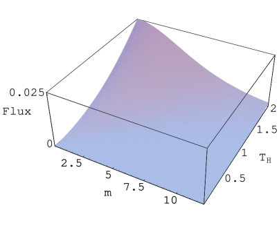
Figure 8: Total Flux for Massive Particles, calculated by the Black Body Hypothesis

For computational reasons I have plotted the flux in a range that is far beyond the interesting physical range. Nevertheless, it shows nicely its qualitative behaviour. For fixed BH mass the flux is almost constant for $m\ll T_{H}$, it falls off exponentially for $m\approx T_{H}$ and it is negligible for $m\gg T_{H}$. Clearly, for a BH in the quasi-static region $M\gg 1$, e.g. $M=M_{\odot}\approx 10^{40}$, the Hawking temperature is extremely small $T_{H}\approx 10^{-40}$ and the interesting region lies at $m\approx 10^{-40}$. Table 6 compares the result of the full quantum calculation (182) with that of the Black Body calculation.

                     $m$ Black Body Field Quantisation $0$ $1.036\cdot 10^{-5}M^{-2}$ - $\frac{1}{10M}$ $5.5\cdot 10^{-6}M^{-2}$ $1.8\cdot 10^{-3}M^{-2}$ $\frac{1}{M}$ $8.8\cdot 10^{-14}M^{-2}$ $1.8\cdot 10^{-5}M^{-2}$ $\frac{1.7}{M}$ $7.2\cdot 10^{-21}M^{-2}$ $6.2\cdot 10^{-6}M^{-2}$ $\frac{2}{M}$ $5.7\cdot 10^{-24}M^{-2}$ $4.5\cdot 10^{-6}M^{-2}$ $\frac{10^{10}}{M}$ $0$ $1.8\cdot 10^{-26}M^{-2}$

                                                         Table 6
In the first line I have listed once more the flux for massless particles (27). The values in the column “Field Quantisation” may be changed crucially if one adds the next perturbative order in $\alpha$. Especially the value at the point $\alpha=1$, where the perturbation series breaks down, might differ drastically from the correct value. Beyond this point the Black Body result goes exponentially fast to zero while the quantum result remains at finite values. Note that the first order of the perturbation series should approach the exact quantum value as $\alpha\to 0$, while its deviation from the Black Body result increases. This disagreement clearly cannot be traced back to the use of the conservation equation because it already concerns the basic components which are derived directly from the effective action (the conservation equation is not changed for massive particles as long as we are in the quasi-static phase $M\gg 1$).

Apart from the missing accordance with the BH radiation law with respect to the qualitative behaviour the result (188) fits nicely to the quantum calculation for massless particles (280). Namely, at the critical point $mM=1$ the flux for massive particles (in this approximation) lies just one order below that of massless particles. This means that, compared to the massless case, the absolute flux is not too high but still contributes with a considerable amount, as expected.

The reason why the behaviour of the expectation value of the EM tensor deviates in such a drastic way from the one suggested by the Black Body law may be found in the very basis of the approach which is the local expansion of the heat kernel. I have shown that this is only possible if the condition $mM\gg 1$ is fulfilled. On the other hand, the estimate (188) demonstrates that this is exactly the range where the flux is effectively zero. Indeed, the point where the exponential damping sets in, namely for $mM\approx 1$ (see Table 6 on the last page), is already out of the scope of the perturbation series which converges for $mM\gg 1$. By this circumstance one cannot describe the physically interesting range, where the BH is still in the quasi-static phase $M>1$ (e.g. $M=10^{10}$) and the geometry can be described accurately by a Schwarzschild spacetime, and where the mass of the scalar particle $m$ lies between $0$ and $\frac{1}{M}$, such that $mM<1$.

I conclude that the local expansion of the heat kernel does not seem appropriate to describe the characteristic features of the radiation of massive particles. Merely, I suppose that the use of the more comprising non-local expansion, see Section 3.2, may reveal the exact behaviour around the critical point $mM\approx 1$. This idea is discussed in the Outlook of my thesis. Nevertheless, the Seeley-DeWitt expansion is the most simple way to derive one-loop expectation values on a curved spacetime in arbitrary dimensions as it does not afford the knowledge of the Green function. In particular, one might use this advantage to compare the two-dimensional dilaton model with the $4d$ theory at the quantum level.

Frolov and Zel’nikov used a similar approach to obtain some of the components of the EM tensor [27]. Their result for the trace and the $T^{\theta}{}_{\theta}$-component is of the same order as mine. Because they derived all components directly from the effective action they could not give an estimate on the radiation component $T^{r}{}_{t}$. If I calculate the radiation constant in the Unruh state by their basic components I obtain $K=-\frac{3.6}{10^{6}\cdot\pi^{2}m^{2}M^{2}}$. Note that they use the inverse sign convention, thus I have multiplied their results by $-1$!

5 Hawking Radiation of Massless Scalars

The main contribution to the Hawking flux of a BH in the quasi-static phase comes from massless particles, namely photons, because their Hawking temperature lies far below the rest mass of the known fundamental massive particles (except probably neutrinos). In the absence of a mass term or in the limit of very low masses the local Seeley-DeWitt expansion of the heat kernel breaks down ($\alpha=\frac{1}{mM}>1$) and the effective action becomes a non-local expression that can be derived by the covariant perturbation theory (Section 3.2). This approach is rather new in the present context and it is more direct and unambiguous as compared to the methods found in the literature [5]. Further, it turns out that the so-called trace anomaly induced effective action, obtained by functional integration of the trace anomaly, only corresponds to (some part of) the first order of the covariant perturbation theory (apart from the fact that this method is not applicable in four dimensions if the scalar field is coupled minimally). The examinations of the last Chapter have shown that the local expansion does not reproduce the significant qualitative behaviour of the Hawking flux for massive particles as it was expected from the Black Body hypothesis. The non-local expansion can therefore be seen as the more comprising case which presumably yields interesting results also for massive scalar fields (I come back to this point in the Outlook).

The non-local effective action, once written down in a compact form, is still difficult to handle. Namely, the non-localities come in by negative powers of Laplacians that can be transformed into multiple integrals over Green functions. Because of their fundamental importance for the effective action I will call these integrals basic integrals. However, the Green functions of a scalar field (massive or massless) on a Schwarzschild spacetime cannot be given in a closed analytical form.

Here emerges the main advantage of the dilaton model: a two-dimensional manifold has only one gravitational degree of freedom, i.e. there is only one independent component of the Riemann tensor. As a consequence the EOM describing the gravitational dynamics of a two-dimensional manifold become integrable and the dynamical evolution is completely determined by the boundary conditions. As a consequence the basic integrals, forming the effective action, can be reduced to boundary terms that are fixed by the boundary conditions of the Green functions. Thereby the IR renormalisation plays a crucial role. The whole Chapter is devoted to the investigation of the dilaton model.

Although the explicit knowledge of the Green functions is not necessary in the dilaton model, I will study the two-point Green functions of massless scalar fields on a two-dimensional Schwarzschild spacetime by a perturbation series, starting from the exactly known Green functions of a flat spacetime. Most importantly, I can show that the perturbation series converges if the Green functions are applied to basic integrals and if the BH interior is excluded from the domain of the Green functions. This is justified by the fact that no classical particles (even those produced in the Hawking effect) can leave the region inside of the horizon – all particles measured as Hawking flux have been produced at or outside the horizon. There are several reasons why it is worthwhile investigating the Green functions: by explicitly calculating the basic integrals one can check consistency of the boundary conditions. Further, I can examine whether the choice of Green function affects the quantum state, as proposed by Barvinsky and Vilkovisky (see the discussion at the end of Section 3.2). Finally, it is likely that these results can be adopted in the four-dimensional theory, where the explicit usage of Green functions is inevitable.

5.1 Dilaton Model

In Section 2.2 I have presented the dilaton model and shown that it is classically equivalent to the s-modes of a scalar field on a four-dimensional Schwarzschild spacetime. In the present Chapter I go one step further and apply the formalism of QFT to the dilaton model. By the methods developed in the Chapters 2 and 3 it will be possible to carry out the whole task of quantising a free scalar field and to obtain the expectation value of the EM tensor to the first order of the perturbation theory.

Before going into details I sketch the procedure:

• First, I establish the non-local effective action of the dilaton model by the covariant perturbation theory to the first perturbational order.

• I discuss the boundary conditions of the Green function and how they affect the basic integrals.

• I derive and discuss the flat retarded and Feynman Green functions and develop a perturbation series for the corresponding Schwarzschild Green functions.

• I calculate the expectation value of the EM tensor and the Hawking flux and discuss the result.

• Finally, I reconsider the effective action with respect to its quantum state and show that an arbitrary quantum state can be fixed by adjusting the constants of the CF approach.

5.2 Effective Action and Expectation Values

In Section 3.2 I have presented the general form of the non-local effective action introduced by Barvinsky and Vilkovisky. Now I want to fix the “parameters” as to describe the dilaton model.

The “parameters” are the spacetime dimension, which from now on is always two $d=2\omega=2$, and the characteristic Euclidean Laplacian ${\cal O}=-\triangle-E$. The dimension of the spacetime always causes a characteristic number, type, and form of IR and UV divergences. As already mentioned, IR divergences are a typical feature of massless particles.

I use the zeta-function regularisation to handle the UV-divergences of the heat kernel. Remember that in this regularisation scheme the effective action was related to the heat kernel as

$$W[g]=-\frac{1}{2}\frac{d\zeta[s]}{ds}\biggm{|}_{s=0}=-\frac{1}{2}\frac{d}{ds}\frac{1}{\Gamma(s)}\int_{0}^{\infty}\frac{d\tau}{\tau^{1-s}}\text{tr}\,e^{-{\cal O}\tau}\biggm{|}_{s=0}.$$ (189)

In the zeta-function the IR-divergent terms are those that behave like $\tau^{-n},\newline n\leq 1$. In any case they demand some additional regularisation (beside the UV-regularisation naturally provided by the zeta-function).

To the second order of the covariant perturbation theory there are five types of terms in the non-local effective action, see (142), with different UV and IR behaviour:

$$\int_{0}^{\infty}\tau^{s-2}d\tau\,,\,\int_{0}^{\infty}\tau^{s-1}d\tau\hskip 241.84842pt$$ (190)

$$\int_{0}^{\infty}\tau^{s}f(-\triangle\tau)d\tau\,,\,\int_{0}^{\infty}\tau^{s-1}\frac{f(-\triangle\tau)-1}{-\triangle}d\tau\,,\,\int_{0}^{\infty}\tau^{s-2}\frac{f(-\triangle\tau)-1}{\triangle^{2}}d\tau.\hskip 14.22636pt$$ (191)

In the integrals in the first line I must introduce an additional IR regularisation by cutting off the upper bound at some value $T$, the other integrals are regularised by the exponential function in $f(-\triangle\tau)$ (141). The first integral does not contribute to the effective action:

$$\frac{d}{ds}\frac{1}{\Gamma(s)}\int_{0}^{T}\tau^{s-2}d\tau\biggm{|}_{s=0}=-\frac{1}{T}\stackrel{{\scriptstyle T\to\infty}}{{\to}}0.$$ (192)

The second integral has a finite and a divergent term:

$$\frac{d}{ds}\frac{1}{\Gamma(s)}\int_{0}^{T}\tau^{s-1}d\tau\biggm{|}_{s=0}=\gamma_{E}+\ln T.$$ (193)

The remaining integrals (191) only lead to finite contributions. This can be seen if I change the order of the $\tau$ and the $a$ integration in the regularised integrals and finally differentiate for $s$ and carry out the limit $s\to 0$. Note that the $1$ in $f(-\triangle\tau)-1$ can be pulled into the integral over $a$ since $1=\int_{0}^{a}1\cdot da$! The first term in (191) after the $\tau$-integration reads

$$\frac{\Gamma(1+s)}{(-\triangle)^{1+s}}\int_{0}^{1}\frac{1}{[a(1-a)]^{1+s}}da\\ =\frac{\Gamma(1+s)}{(-\triangle)^{1+s}}\int_{-1/2}^{1/2}\frac{(-1)^{1+s}}{\left[u^{2}-\frac{1}{4}\right]^{1+s}}du=\frac{2^{1+2s}\sqrt{\pi}\cdot\Gamma(1+s)\Gamma(-s)}{(-\triangle)^{1+s}\Gamma(\frac{1}{2}-s)}.$$ (194)

The other two integrals in (191) can be treated analogously. The contribution of these three terms to the effective action reads

$$\frac{d}{ds}\frac{1}{\Gamma(s)}\int_{0}^{\infty}\tau^{s}f(-\triangle\tau)d\tau\biggm{|}_{s=0} = \frac{2\cdot\ln(-\triangle)}{-\triangle}$$ (195)

$$\frac{d}{ds}\frac{1}{\Gamma(s)}\int_{0}^{\infty}\tau^{s-1}\frac{f(-\triangle\tau)-1}{-\triangle}d\tau\biggm{|}_{s=0} = \frac{2-\ln(-\triangle)}{-\triangle}$$ (196)

$$\frac{d}{ds}\frac{1}{\Gamma(s)}\int_{0}^{\infty}\tau^{s-2}\frac{f(-\triangle\tau)-1}{\triangle^{2}}d\tau\biggm{|}_{s=0} = \frac{\ln(-\triangle)-\frac{8}{3}}{6(-\triangle)}.$$ (197)

Now I have all pieces at hand to construct the effective action for a general two-dimensional scalar model. Putting together these results, the formula for the heat kernel (142), and the defining equation of the effective action (104) I obtain

$$W_{\cal E}[g]=\frac{1}{96\pi}\int_{L}\biggm{[}-(2R+12E)(\gamma_{E}+\ln T)\\ +(R+12E)\frac{1}{\triangle}R+2R\frac{\ln(-\triangle)}{\triangle}E-2E\frac{\ln(-\triangle)}{\triangle}R\biggm{]}\sqrt{g}d^{2}x.$$ (198)

The last two terms vanish if I consider commuting fields as in this case also the scalar curvature and the endomorphism commute, i.e. $RE=ER$. The logarithm in the last term can then be expanded in a power series and by partial integration the Laplacians of this series can be made acting on $E$ without a change of sign (the surface terms vanish if I assume that $M$ is flat in the infinite future and past).

The very first term in the effective action must be renormalised in any case. I define a renormalisation constant $c_{R}:=\gamma_{E}+\ln T$ that I fix later by the physical requirements of the EM tensor.

Now I go over to the Lorentzian effective action:

$$W_{\cal M}[g]=\frac{1}{96\pi}\int_{L}\left[-c_{R}(2R-12\varepsilon_{\cal E}E_{\cal M})+(R-12\varepsilon_{\cal E}E_{\cal M})\frac{1}{\square}R\right]\sqrt{-g}d^{2}x.$$ (199)

Note that beside $R\to-R,\triangle\to-\square$ we have $W_{M}=iW_{E}$ and $d\tau=idt$. This action is in fact of the most general form for all commuting scalar fields. It covers all kinds of couplings and potentials that are specified by the Laplacian and the associated endomorphism.

Now I will examine how the dilaton model (66) can be described by this effective action (at the quantum level). The Lorentzian Laplacian reads

$${\cal O}_{\cal M}=X\square+(\nabla X)\nabla.$$ (200)

To bring it into the standard form I must define a conformally related metric $\hat{g}^{\alpha\beta}=Xg^{\alpha\beta}$:

$${\cal O}_{\cal M}=\left(\hat{\nabla}+\frac{\hat{\nabla}X}{2X}\right)\left(\hat{\nabla}+\frac{\hat{\nabla}X}{2X}\right)+\frac{(\hat{\nabla}X)^{2}}{4X^{2}}-\frac{\hat{\square}X}{2X}=\hat{\square}_{tot}+\frac{(\nabla X)^{2}}{4X}-\frac{\square X}{2}$$ (201)

$\hat{\square}_{tot}$ is the total geometric Laplacian, hence I must replace all geometric objects in the effective action by those associated to the connection $\hat{\nabla}_{tot}=\hat{\nabla}+\frac{\hat{\nabla}X}{2X}$, whereby I can omit the “gauge part” $\frac{\hat{\nabla}X}{2X}$ because of its commutativity (see Appendix F.1 (460)):

$$\Omega_{ab}S=[\hat{\nabla}^{tot}_{a},\hat{\nabla}^{tot}_{b}]S=[\hat{\nabla}_{a},\hat{\nabla}_{b}]S+\left(\hat{\nabla}_{[a}\hat{\nabla}_{b]}\ln X\right)S=0.$$ (202)

The Lorentzian endomorphism from (201) reads

$$E_{\cal M}=\frac{(\nabla X)^{2}}{4X}-\frac{\square X}{2}$$ (203)

and exhibits an Euclidean sign $\varepsilon_{\cal E}(E)=-1$. Further, I have to replace the scalar curvature by $\hat{R}=XR-\frac{(\nabla X)^{2}}{X}+\square X$ and the volume element by $\sqrt{-\hat{g}}=X^{-1}\sqrt{-g}$, see Appendix C (409,405). Hence the non-local part of the effective action (198) has the form

$$W_{nl}[g]=\frac{1}{96\pi}\int_{L}(X^{-1}\sqrt{-g})\left[XR-\frac{(\nabla X)^{2}}{X}+\square X+12E_{\cal M}\right]\\ \cdot\frac{1}{X\square}\left[XR-\frac{(\nabla X)^{2}}{X}+\square X\right]d^{2}x\\ =-\frac{1}{96\pi}\int_{L}\left[R+2\frac{(\nabla X)^{2}}{X^{2}}-5\frac{\square X}{X}\right]\\ \cdot\int^{\prime}_{L}G(x,x^{\prime})\left[R^{\prime}-\frac{(\nabla X^{\prime})^{2}}{(X^{\prime})^{2}}+\frac{\square^{\prime}X^{\prime}}{X^{\prime}}\right]\sqrt{-g^{\prime}}d^{2}x^{\prime}\sqrt{-g}d^{2}x.$$ (204)

In the second line I have again replaced the negative power of the geometric Laplacian by an integral over a Green function: $\frac{1}{\square}=-\int^{\prime}_{L}G(x,x^{\prime})\sqrt{-g^{\prime}}d^{2}x^{\prime}$.

The local part of the effective action reads

$$W_{l}[g]=\frac{1}{96\pi}\int_{L}(-c_{R})\left[2R+\frac{(\nabla X)^{2}}{X^{2}}-\frac{\square X}{X}\right]\sqrt{-g}d^{2}x.$$ (205)

Now it is convenient to introduce the field $\phi$ by $X=e^{-2\phi}$. This gives the identities

$$\frac{(\nabla X)^{2}}{X^{2}}=4(\nabla\phi)^{2}\,\,,\,\,\frac{\square X}{X}=4(\nabla\phi)^{2}-2\square\phi.$$ (206)

The non-local part of the effective action then becomes

$$W_{nl}[g]=-\frac{1}{96\pi}\int_{L}[R-12(\nabla\phi)^{2}+10\square\phi]\\ \cdot\int^{\prime}_{L}G(x,x^{\prime})[R^{\prime}-2\square^{\prime}\phi^{\prime}]\sqrt{-g^{\prime}}d^{2}x^{\prime}\sqrt{-g}d^{2}x.$$ (207)

In this form the effective action, together with the local part, allows to derive all one-loop expectation values of the scalar field $S$ in the dilaton model. The non-local part represents the second order of the covariant perturbation series (134) – higher orders (corresponding to further curvature lines in Figure 5) would appear in the form of multiply staggered integrals. The information on the scalar field provided by the effective action is hidden in the Green functions. Their knowledge, beside the geometric data of the manifold given by $R$ and $\phi$, is the key to the expectation values.

In two dimensions the situation is very particular. Namely, the geometric variables only possess one dynamical field degree of freedom. This implies that all geometric objects can be described by just one variable. So the scalar curvature $R$ already determines the complete Riemann tensor. Further, one can find a representation of the metric where its component matrix is a multiple of the flat metric $\eta_{\alpha\beta}=\text{diag}(1,-1)$: $g_{\alpha\beta}=e^{2\rho}\eta_{\alpha\beta}$. This representation is called the conformal gauge, see Appendix A.3. In this gauge the scalar curvature can be written as $R=-2\square\rho$. If I substitute this into the effective action I can perform the $x^{\prime}$-integration and obtain a completely local effective action:

$$W[g]=\frac{1}{24\pi}\int_{L}\Bigm{\{}-3c_{R}(\nabla\phi)^{2}+[\square\rho+6(\nabla\phi)^{2}-5\square\phi][\rho+\phi]\Bigm{\}}\sqrt{-g}d^{2}x.$$ (208)

This result is obtained by setting $\square^{-1}\square=1$ in the non-local action. Thereby I have dropped a homogeneous solution $\chi$ of the Laplace equation $\square\chi=0$. Generally, for a function $f(x)$, we would have

$$\int_{L}G(x,x^{\prime})\square f(x)\sqrt{-g}d^{2}x=-\frac{1}{\square}\square f=-\frac{1}{\square}\square(f+\chi)=-(f+\chi).$$ (209)

By looking to the l.h.s. and the r.h.s. of this equation we see that $\chi$ (as a function of $x$) is determined uniquely by the Green function in the integral. It will be the subject of the next Section to show that $\chi$ is indeed zero for the considered integrals and therefore (208) is the appropriate effective action for my purposes.

It will turn out that the Hawking flux is independent of the (originally) local term in the action and hence of the renormalisation constant $c_{R}$. Nevertheless, it cannot be chosen arbitrarily because it affects other components of the EM tensor like the energy density. In the CF approach it appears in the $T^{\theta}{}_{\theta}$-component of the EM tensor in the same place like the homogeneous solution $\chi$, hence, if the latter is only a constant (as it will be the case), it can be removed by the renormalisation term. For the moment I will disregard this term by setting $c_{R}=0$.

A final Remark: The effective action (208) differs from the one derived in [5]. The difference can be traced back to a different choice of path integral measure and a field redefinition in the four-dimensional effective action (36). In a first step a factor $\sqrt[4]{-g}$ is introduced into the path integral measure $Z[g]={\cal N}^{\prime}\int{\cal D}(\sqrt[4]{-g}S)\cdot e^{iL_{m}[g,S]}$ [28]. This does clearly not affect the expectation values because there the normalisation drops out. Then a new field is defined by $S^{\prime}:=S\sqrt[4]{-g}$ and the classical action becomes $L^{\prime}=-\int S^{\prime}\square S^{\prime}d^{2}x$. Note that neither the new field $S^{\prime}$ nor the volume element $d^{4}x$ are diffeomorphism invariant anymore! The action is spherically reduced by introducing the spherically reduced Laplacian $\square_{4}=\square_{2}+\frac{\nabla X}{X}\nabla$ (see Appendix D (449)) and by integration over the angular coordinates $\theta,\varphi$. One can construct the corresponding non-local effective action by the same steps as before. Things are a bit easier now because the geometric Laplacian is simply $\triangle$, the metric must not be conformally transformed, and the endomorphism becomes $E_{\cal M}=\frac{(\nabla X)^{2}}{4X^{2}}-\frac{\square X}{2X}=-(\nabla\phi)^{2}+\square\phi$. In its local form the effective action reads $W^{\prime}[g]=\frac{1}{24\pi}\int_{L}\left\{-3c_{R}(\nabla\phi)^{2}+\rho\square\rho+6\rho(\nabla\phi)^{2}-6\rho\square\phi\right\}\sqrt{-g}d^{2}x$ which is identical to the effective action derived in [5]. $c_{R}$ is again a renormalisation constant that does not affect the Hawking flux. Therefore, the basic components and hence the Hawking flux agree with those of [5]: $\left<T\right>_{2}=\frac{M}{3\pi r^{3}}\,,\left<T^{\theta}{}_{\theta}\right>_{2}=-\frac{1}{8\pi r^{5}}\left\{4M+(4M-r)\left[\ln\left(1-\frac{2M}{r}\right)-c_{R}\right]\right\},\left<T^{r}{}_{t}\right>_{2}=\frac{1}{768\pi M^{2}}$. Interestingly, the flux agrees with (280), the one calculated in this thesis from (208), although all other components of the EM tensor differ.

5.3 Boundary Conditions

In the local form of the effective action (208) the boundary conditions have already been fixed implicitly by the assumption $\square^{-1}\square=1$. As already mentioned above one might have an additional contribution by a homogeneous Green function. This contribution corresponds to a boundary term that can be fixed by the boundary conditions imposed on the Green functions. This can be studied best by Green’s theorem in curved spacetime

$$\int_{V}\Bigm{[}f(x^{\prime})\square^{x^{\prime}}G(x,x^{\prime})-G(x,x^{\prime})\square^{x^{\prime}}f(x^{\prime})\Bigm{]}\sqrt{-g^{\prime}}d^{2}x^{\prime}\\ =\oint_{\partial V}\Bigm{[}f(x^{\prime})\nabla_{\alpha}^{x^{\prime}}G(x,x^{\prime})-G(x,x^{\prime})\nabla_{\alpha}^{x^{\prime}}f(x^{\prime})\Bigm{]}\sqrt{-g^{\prime}}\cdot g^{\alpha\beta}\varepsilon_{\beta\gamma}(dx^{\prime})^{\gamma}.$$ (210)

If I apply it to the basic integrals in the effective action, where $F=\square f$, I can express the non-localities by the sum of a local term and a boundary term:

$$-\frac{1}{\square}F=\int_{L}G(x,x^{\prime})F(x^{\prime})\sqrt{-g^{\prime}}d^{2}x^{\prime}\\ =-f(x)-\oint_{\partial L}\Bigm{[}f\nabla_{\alpha}^{\prime}G-G\nabla_{\alpha}^{\prime}f\Bigm{]}\sqrt{-g^{\prime}}\varepsilon^{\alpha}{}_{\beta}(dx^{\prime})^{\beta}\\ =-f(x)-\int_{2M}^{\infty}f(x^{\prime})\partial_{t^{\prime}}G\frac{dr^{\prime}}{\left(1-\frac{2M}{r^{\prime}}\right)}\biggm{|}_{t^{\prime}=\infty}+\,{\dots}\biggm{|}_{t^{\prime}=-\infty}\\ -\int_{-\infty}^{\infty}\Big{[}f(x^{\prime})\partial_{r^{\prime}}G-G\partial_{r^{\prime}}f(x^{\prime})\Big{]}\left(1-\frac{2M}{r^{\prime}}\right)dt^{\prime}\biggm{|}_{r^{\prime}=2M}+\,{\dots}\biggm{|}_{r^{\prime}=\infty}.$$ (211)

One immediately observes that the boundary terms in the third line are not well-defined if $G$ does not vanish at least linearly at $r^{\prime}=2M$ (for arbitrary $x$). If this is provided, the function $f$ may still have a logarithmic divergence on the horizon (as it is the case with the conformal metric factor $\rho$). This trouble can be traced back to the fact that the Schwarzschild coordinates break down at the horizon. In fact, from the point of view of this gauge the spacetime must be considered as to end at the horizon, and the two-dimensional spacetime spanned by $t,r$ is thus isomorphic to a rectangle $\{-\infty,\infty\}\times\{2M,\infty\}$ in coordinate space. Therefore one is forced to fix boundary conditions on the horizon, namely by demanding that the eigenfunctions of the Laplace operator, and hence the Green functions, vanish there. According to the reasoning in the introduction of this Chapter the usage of Schwarzschild coordinates seems to be appropriate to calculate the Hawking flux.

In (211) one also can see the possible IR problems, caused by the fact that the Green functions of massless particles do not have a sufficient fall-off behaviour for large point-separations $|x-x^{\prime}|$. The physical picture is the following: the measurement of the Hawking flux takes place somewhere at a finite distance from the BH and at some instant of time during the quasi-static phase, i.e. when the BH mass is much larger than the Planck mass $M\gg 1$. Hence, only particles with effectively zero energy can contribute to this expectation value by travelling from infinity until the point of measurement – such particles clearly are a mathematical idealization as physical particles always possess a minimum energy, therefore their (formally infinite) contribution must be renormalised to zero. This can be achieved by several methods. The most obvious way is to introduce a mass of the scalar particle such that the Green functions become exponentially damped. The boundary terms then vanish and afterwards the mass can be set to zero; the elimination of the boundary terms in (211) represents the only difference to the unrenormalised case. Or one can work with a finite spacetime volume, by limiting the range of the coordinates to finite values, and allows only wave lengths that fit into this rectangular of finite size. Thereby one singles out those eigenfunctions that vanish (at least linearly) on the boundary and hence the Green functions inherit this boundary condition. Note that these Green functions naturally vanish also on the horizon as it belongs to the boundary. The same happens by the introduction of a mass term because particles with a finite mass need an infinite time to reach or leave the horizon!

By these considerations I conclude that any possible contribution from the boundaries of the manifold (including the event horizon) are unphysical and must be removed by some infrared renormalisation. The easiest way to realize this in practical calculations is to drop all boundary terms if the integrand contains a Green function and the remaining integrand is at most logarithmically divergent on the boundary. This procedure will be one of the basic ingredients in the Green function perturbation theory of the next Section.

By applying this renormalisation prescription to (211) all boundary terms cancel (the spacelike terms in the third line are finite on the horizon and vanish because they are in the remote past, respectively future) if $f$ has at most logarithmic divergences. For such functions the relation

$$\square^{-1}\square=1$$ (212)

is indeed valid. In the effective action one has instead of $f$ the functions $\rho=\frac{1}{2}\ln\sqrt{1-\frac{2M}{r}}$ and $\varphi=-\ln r$ which fulfil the necessary regularity condition. Thus, (208) is the unique local form of the effective action that is compatible with the required IR renormalisation. Further, as the Green function only appears in the boundary terms, the effective action, and accordingly the expectation values, is independent of the type of Green function.

5.4 Green Function Perturbation

In Section 5.2 I have used the conformal gauge to render the effective action local. Thereby I have thrown away a homogeneous solution $\chi$ of the geometric Laplace equation. In the last Section I have shown that the IR renormalisation justifies this step as it removes the boundary terms that correspond to this homogeneous solution. In principle, this would be enough to guarantee the existence of a unique local form of the effective action and hence the uniqueness of the expectation values derived from it.

Apart from the fact that the Hawking flux of massless particles in the dilaton model can be calculated without knowing explicitly the Green function of the two-dimensional Schwarzschild Laplacian, there are several reasons to examine them. Basically, it would be interesting to know if the considerations on the boundary terms can be affirmed by a direct calculation. Further, by explicitly dealing with the Green functions one can choose between different types among them and investigate their effect (or not existing effect) on the basic integrals. Finally, the method developed in this Section may be a guiding line for the investigations in four dimensions.

The procedure presented here is strongly adapted as to examine the specific types of basic integrals that appear in the non-local effective action. Beside the IR renormalisation discussed in the last Section, also the fact that the perturbative Green function is applied to the basic integrals will be crucial for its convergence.

The objects of my investigations will be integrals of the type

$$\int G(x,x^{\prime})F(r^{\prime})\sqrt{-g^{\prime}}d^{2}x^{\prime}=\int G(x,x^{\prime})\square^{\prime}f(r^{\prime})\sqrt{-g^{\prime}}d^{2}x^{\prime}=-[f(r)+\chi_{f}(r)],$$ (213)

that I call basic integrals. The functions $F,f,\chi$, and hence the whole equation shall be time-independent. For $F$ and $f$ this is just the static approximation, i.e. I approximate the BH spacetime in the slowly evolving region by a Schwarzschild BH. As a result the basic integrals themselves will be time-independent (as it can be seen from the explicit calculations in Section 5.6.2). Thus, also $\chi$ must be time-independent. The general time-independent solutions of the homogeneous Laplace equation $\square\chi$ (on a Schwarzschild background) can be written as

$$\chi_{f}=C_{1}^{f}+C_{2}^{f}\frac{r_{\ast}}{2M}=C_{1}^{f}+C_{2}^{f}\left[\frac{r}{2M}+\ln\left(\frac{r}{2M}-1\right)\right],$$ (214)

where $r_{\ast}$ is the Tortoise coordinate, see Appendix A.3. In Section 5.6.2 I will show that the Hawking flux and all other components of the EM tensor are not affected by the constant $C_{1}^{f}$. Nevertheless it is formally useful because it connects my results to the ones in the literature by an infinite constant that appears in the perturbation series of the Green functions – I have always the freedom to add such a constant without changing measurable quantities.

The Green functions, even of the two-dimensional Laplace operator on a Schwarzschild spacetime fulfilling the equation

$$\square G(x,x^{\prime})=-\delta(x-x^{\prime}),$$ (215)

are not known in a closed analytical form. Also the eigenfunctions of the Laplace operator are not known exactly, therefore one cannot proceed as usual and construct the Green functions by their decomposition into eigenfunctions. For this reason I cannot solve the basic integrals analytically.

From equations (213,214) one can see that the asymptotic behaviour (i.e. for large values of the radius $r$) of the basic integrals is sufficient to determine the constant $C_{2}^{f}$. This encourages me to approximate the exact Green function by the one from flat spacetime $G_{0}(x,x^{\prime})$ and introduce a perturbation series to calculate the next order approximations.

The perturbation series has the form

$$G(x,x^{\prime})=G_{0}(x,x^{\prime})+\int^{\prime\prime}_{L}G_{0}(x,x^{\prime\prime})\delta\square^{\prime\prime}G_{0}(x^{\prime\prime},x^{\prime})d^{2}x^{\prime\prime}\\ +\int^{\prime\prime}_{L}\int^{\prime\prime\prime}_{L}G_{0}(x,x^{\prime\prime})\delta\square^{\prime\prime}G_{0}(x^{\prime\prime},x^{\prime\prime\prime})\delta\square^{\prime\prime\prime}G_{0}(x^{\prime\prime\prime},x^{\prime})d^{2}x^{\prime\prime}d^{2}x^{\prime\prime\prime}+\dots,$$ (216)

where $\delta\square=\square-\square_{0}$ is the perturbing Laplacian and $\square_{0}=\partial_{t}^{2}-\partial_{r}^{2}$ is the flat Laplacian. When computing more complicated expressions I will use the notation $G_{0}(x,x^{\prime})=G^{x}_{{}^{\prime}}$ (only for the flat Laplacian!) and $f(x)=f^{x},f(x^{\prime\prime})=f^{\prime\prime}$. Further, I will omit the volume element $d^{2}x$ and the index $L$ of the integrals. That (216) is a Green function of the full Laplacian $\square$ can be seen immediately:

$$\square^{x}G(x,x^{\prime})=\square^{x}G^{x}_{{}^{\prime}}-\delta\square^{x}G^{x}_{{}^{\prime}}+\int^{\prime}\delta\square^{x}G^{x}_{{}^{\prime\prime}}\delta\square^{\prime\prime}G^{\prime\prime}_{{}^{\prime}}\\ -\int^{\prime\prime\prime}\delta\square^{x}G^{x}_{{}^{\prime\prime\prime}}\delta\square^{\prime\prime\prime}G^{\prime\prime\prime}_{{}^{\prime}}+\int^{\prime\prime}\int^{\prime\prime\prime}\delta\square^{x}G^{x}_{{}^{\prime\prime}}\delta\square^{\prime\prime}G^{\prime\prime}_{{}^{\prime\prime\prime}}\delta\square^{\prime\prime\prime}G^{\prime\prime\prime}_{{}^{\prime}}+\dots{\\ }=\square_{0}G^{x}_{{}^{\prime}}=-\delta(x-x^{\prime}).$$ (217)

The series converges if the condition

$$\left|\int^{\prime\prime}\delta\square^{\prime\prime}G_{0}(x^{\prime\prime},x^{\prime})\right|<1$$ (218)

is fulfilled. In the following I will discuss when this is the case. I can write the perturbed Laplacian in the form (remember that $\square=\left(1-\frac{2M}{r}\right)^{-1}\partial_{t}^{2}-\partial_{r}[\left(1-\frac{2M}{r}\right)\partial_{r}]$)

$$\delta\square=\frac{2M}{r-2M}\partial_{t}^{2}+\partial_{r}\left(\frac{2M}{r}\partial_{r}\right).$$ (219)

Before starting with the estimate I emphasize some critical points. From (219) it is obvious that condition (218) cannot be fulfilled in the general case. But as I will only apply the Green functions in the basic integrals I can make use of the time-independence of the latter. Second, I will restrict the range of the $r$-integration to the horizon, i.e. the radius-coordinate $r$ will only be integrated from $2M$ to $\infty$, and employ the boundary conditions as discussed in the last Section.

I will put some function $f(r)$ into the integral of (218). This makes the calculation more transparent and corresponds to the application of the perturbation series to a basic integral. If I write a partial derivative without coordinate index this will always mean differentiation for $r$, e.g. $\partial^{\prime\prime}=\partial_{r^{\prime\prime}}$.

$$\int^{\prime}f^{\prime}\frac{2M}{r^{\prime}-2M}\partial_{t^{\prime}}^{2}G^{\prime}_{x}+\int^{\prime}f^{\prime}\partial^{\prime}\left(\frac{2M}{r^{\prime}}\partial^{\prime}G^{\prime}_{x}\right)\\ =\partial_{t}^{2}\int^{\prime}f^{\prime}\frac{2M}{r^{\prime}-2M}G^{\prime}_{x}+\int^{\prime}\partial^{\prime}\left(f^{\prime}\frac{2M}{r^{\prime}}\partial^{\prime}G^{\prime}_{x}\right)-\int^{\prime}(\partial^{\prime}f^{\prime})\frac{2M}{r^{\prime}}\partial^{\prime}G^{\prime}_{x}\\ =-\int^{\prime}(\partial^{\prime}f^{\prime})\frac{2M}{r^{\prime}}\partial^{\prime}G^{\prime}_{x}.$$ (220)

I have used the relations $\partial_{t}G_{0}(x,x^{\prime})=-\partial_{t^{\prime}}G_{0}(x,x^{\prime}),\partial_{t}^{2}G_{0}(x,x^{\prime})=\partial_{t^{\prime}}^{2}G_{0}(x,x^{\prime})$ and $\partial_{r}G_{0}(x,x^{\prime})=\partial_{r^{\prime}}G_{0}(x,x^{\prime})$ (see the Fourier-transform of the flat Green functions in the next Sections (229)). Hence I can pull the time-derivative in the first line out of the integral and it becomes zero because of its time-independence (see below). The factor $(r^{\prime}-2M)^{-1}$ does not cause problems because $G_{0}$ vanishes on the horizon. The surface term in the second line vanishes by the boundary conditions (the $r^{\prime}$-derivative of $G_{0}$ can be transformed into an $r$-derivative). Now I consider the identity

$$f(r)=-\int^{\prime}f^{\prime}\square_{0}^{\prime}G^{\prime}_{x}=\int^{\prime}f^{\prime}(\partial_{r^{\prime}}^{2}-\partial_{t^{\prime}}^{2})G^{\prime}_{x}\\ =-\partial_{t}^{2}\int^{\prime}f^{\prime}G^{\prime}_{x}+\int^{\prime}\partial^{\prime}(f^{\prime}\partial^{\prime}G^{\prime}_{x})-\int^{\prime}(\partial^{\prime}f^{\prime})\partial^{\prime}G^{\prime}_{x}=-\int^{\prime}(\partial^{\prime}f^{\prime})\partial^{\prime}G^{\prime}_{x}.$$ (221)

Obviously the absolute value of this integral is larger than that of (220). Thus I have the inequality

$$\left|\int^{\prime\prime}f(r^{\prime\prime})\delta\square^{\prime\prime}G_{0}(x^{\prime\prime},x^{\prime})\right|<f(r^{\prime})$$ (222)

which proves the convergence of the perturbation series if applied to time-independent functions in basic integrals.

5.4.1 Second and Third Order

In this Section I will bring the second and third order of the perturbation series in a simple form, such that the basic integrals can be solved by simple integrations if the flat Green functions are known. Again I will assume that the basic integrals are time-independent, hence all terms with time-derivatives do not contribute. Further, I will use the boundary condition that $G$ vanishes on the boundary of the manifold (that begins at $r=2M$).

The second order of the perturbation then reads

$$-\int^{\prime\prime}[\partial_{r^{\prime\prime}}G_{0}(x,x^{\prime\prime})]\frac{2M}{r^{\prime\prime}}\partial_{r^{\prime\prime}}G_{0}(x^{\prime\prime},x^{\prime})d^{2}x^{\prime\prime},$$ (223)

where I have partially integrated one $r^{\prime\prime}$-derivative. I define the function

$$g(r):=\frac{2M}{r}.$$ (224)

Note that $\partial_{r}^{2}g(r)=-R(r)$ on a two-dimensional Schwarzschild spacetime. Now I derive a useful identity, introducing light-cone derivatives $\partial_{\pm}=\partial_{t}\pm\partial_{r}$ , $\square_{0}=\partial_{+}\partial_{-}=\partial_{-}\partial_{+}$. Note that because of the time-independence I can effectively set $\square_{0}=-\partial_{r}^{2}$ and $\partial_{+}=-\partial_{-}=\partial_{r}$. Again I use the notation $\partial^{\prime}=\partial_{r^{\prime}}$.

$$0=\int^{\prime\prime}\square_{0}^{\prime\prime}(G^{x}_{{}^{\prime\prime}}G^{\prime\prime}_{{}^{\prime}}g^{\prime\prime})\\ =\int^{\prime\prime}\left\{g^{\prime\prime}\square_{0}^{\prime\prime}(G^{x}_{{}^{\prime\prime}}G^{\prime\prime}_{{}^{\prime}})-\partial^{\prime\prime}(G^{x}_{{}^{\prime\prime}}G^{\prime\prime}_{{}^{\prime}})\partial^{\prime\prime}g^{\prime\prime}-\partial^{\prime\prime}(G^{x}_{{}^{\prime\prime}}G^{\prime\prime}_{{}^{\prime}})\partial^{\prime\prime}g^{\prime\prime}-(G^{x}_{{}^{\prime\prime}}G^{\prime\prime}_{{}^{\prime}})(\partial^{\prime\prime})^{2}g^{\prime\prime}\right\}\\ =\int^{\prime\prime}\left\{g^{\prime\prime}[-\delta(x,x^{\prime\prime})G^{\prime\prime}_{{}^{\prime}}-\delta(x^{\prime\prime},x^{\prime})G^{x}_{{}^{\prime\prime}}-2(\partial^{\prime\prime}G^{x}_{{}^{\prime\prime}})\partial^{\prime\prime}G^{\prime\prime}_{{}^{\prime}}]+(G^{x}_{{}^{\prime\prime}}G^{\prime\prime}_{{}^{\prime}})(\partial^{\prime\prime})^{2}g^{\prime\prime}\right\}\\ =-gG^{x}_{{}^{\prime}}-g^{\prime}G^{x}_{{}^{\prime}}-\int^{\prime\prime}\left\{(G^{x}_{{}^{\prime\prime}}G^{\prime\prime}_{{}^{\prime}})R^{\prime\prime}+2g^{\prime\prime}(\partial^{\prime\prime}G^{x}_{{}^{\prime\prime}})\partial^{\prime\prime}G^{\prime\prime}_{{}^{\prime}}\right\}$$ (225)

By this identity the second order of the perturbation series can be written in the compact form

$$\frac{1}{2}\left\{[g(r)+g(r^{\prime})]G_{0}(x,x^{\prime})+\int^{\prime\prime}G_{0}(x,x^{\prime\prime})G_{0}(x^{\prime\prime},x^{\prime})R(r^{\prime\prime})d^{2}x^{\prime\prime}\right\}.$$ (226)

In a similar manner I can compute the third order:

$$\int^{\prime\prime}\int^{\prime\prime\prime}G^{x}_{{}^{\prime\prime}}\partial^{\prime\prime}(g^{\prime\prime}\partial^{\prime\prime}G^{\prime\prime}_{{}^{\prime\prime\prime}})\partial^{\prime\prime\prime}(g^{\prime\prime\prime}\partial^{\prime\prime\prime}G^{\prime\prime\prime}_{{}^{\prime}})=\int^{\prime\prime}(\partial^{\prime\prime}G^{x}_{{}^{\prime\prime}})g^{\prime\prime}\partial^{\prime\prime}\int^{\prime\prime\prime}(\partial^{\prime\prime\prime}G^{\prime\prime}_{{}^{\prime\prime\prime}})g^{\prime\prime\prime}\partial^{\prime\prime\prime}G^{\prime\prime\prime}_{{}^{\prime}}\\ =-\frac{1}{2}\int^{\prime\prime}(\partial^{\prime\prime}G^{x}_{{}^{\prime\prime}})g^{\prime\prime}\partial^{\prime\prime}\left\{(g^{\prime\prime}+g^{\prime})G^{\prime\prime}_{{}^{\prime}}+\int^{\prime\prime\prime}G^{\prime\prime}_{{}^{\prime\prime\prime}}G^{\prime\prime\prime}_{{}^{\prime}}R^{\prime\prime\prime}\right\}\\ =\frac{1}{4}\left\{[g^{2}+(g^{\prime})^{2}]G^{x}_{{}^{\prime}}-\int^{\prime\prime}G^{x}_{{}^{\prime\prime}}G^{\prime\prime}_{{}^{\prime}}(\partial^{\prime\prime})^{2}(g^{\prime\prime})^{2}-\int^{\prime\prime}(\partial^{\prime\prime}G^{x}_{{}^{\prime\prime}})G^{\prime\prime}_{{}^{\prime}}\partial^{\prime\prime}(g^{\prime\prime})^{2}\right\}\\ -\frac{g^{\prime}}{2}\int^{\prime\prime}(\partial^{\prime\prime}G^{x}_{{}^{\prime\prime}})g^{\prime\prime}\partial^{\prime\prime}G^{\prime\prime}_{{}^{\prime}}-\frac{1}{2}\int^{\prime\prime\prime}G^{\prime\prime\prime}_{{}^{\prime}}R^{\prime\prime\prime}\int^{\prime\prime}(\partial^{\prime\prime}G^{x}_{{}^{\prime\prime}})g^{\prime\prime}\partial^{\prime\prime}G^{\prime\prime}_{{}^{\prime\prime\prime}}\\ =\frac{1}{4}\biggm{\{}[g^{2}+(g^{\prime})^{2}]G^{x}_{{}^{\prime}}+\int^{\prime\prime}G^{x}_{{}^{\prime\prime}}[\partial^{\prime\prime}(g^{\prime\prime})^{2}]\partial^{\prime\prime}G^{\prime\prime}_{{}^{\prime}}+[g^{\prime}g+(g^{\prime})^{2}]G^{x}_{{}^{\prime}}+g^{\prime}\int^{\prime\prime}G^{x}_{{}^{\prime\prime}}G^{\prime\prime}_{{}^{\prime}}R^{\prime\prime}\\ +\int^{\prime\prime\prime}G^{\prime\prime\prime}_{{}^{\prime}}R^{\prime\prime\prime}\left([g+g^{\prime\prime\prime}]G^{x}_{{}^{\prime\prime\prime}}+\int^{\prime\prime}G^{x}_{{}^{\prime\prime}}G^{\prime\prime}_{{}^{\prime\prime\prime}}R^{\prime\prime}\right)\biggm{\}}.$$ (227)

Here I have used again identity (225). Finally, I write down the third order of the perturbation series in a compact form, replacing $\partial_{r}g^{2}(r)=2R(r)$:

$$\frac{1}{4}\biggm{\{}[g^{2}(r)+g(r)g(r^{\prime})+2g^{2}(r^{\prime})]G_{0}(x,x^{\prime})\\ +\int^{\prime\prime}G_{0}(x,x^{\prime\prime})R(r^{\prime\prime})[2\cdot\partial_{r^{\prime\prime}}+g(r^{\prime})]G_{0}(x^{\prime\prime},x^{\prime})d^{2}x^{\prime\prime}\\ +\int^{\prime\prime\prime}G_{0}(x^{\prime\prime\prime},x^{\prime})R(r^{\prime\prime\prime})\\ \cdot\left([g(r)+g(r^{\prime\prime\prime})]G_{0}(x,x^{\prime\prime\prime})+\int^{\prime\prime}G_{0}(x,x^{\prime\prime})G_{0}(x^{\prime\prime},x^{\prime\prime\prime})R(r^{\prime\prime})d^{2}x^{\prime\prime}\right)d^{2}x^{\prime\prime\prime}\biggm{\}}.$$ (228)

5.5 Flat Green Functions

The flat Green functions on the half-plane are the basis of the perturbation series. I will derive the Feynman Green function $G_{F}$ and the retarded Green function $G_{ret}$ by choosing different integration paths in the Fourier decomposition of the Green functions. At the end of Section 3.2 I have mentioned the suggested relation between $G_{F}$ and the $\left|H\right>$-state and between $G_{ret}$ and the $\left|U\right>$-state. From the physical point of view $\left|U\right>$ is more interesting as it is the vacuum state and describes a radiating BH surrounded by empty space. However, the Euclidean origin of the effective action suggests to use the Feynman Green function. As I have proofed in Section 2.4.2, the expectation values of the basic components $\left<T\right>,\left<T^{\theta}{}_{\theta}\right>$ which I compute by the effective action are state-independent, hence I could use any Green function corresponding to a sensible physical quantum state. Nevertheless, I consider $G_{F}$ and $G_{ret}$ as to investigate the proposed correspondence between quantum states and Green functions.

5.5.1 Retarded and Feynman Green Functions on the Half-Plane

All Green functions can be expressed by their Fourier decomposition into eigenfunctions $e^{ikx}$ of the flat Laplacian $\square_{0}$. I will first calculate the Green functions on the half-plane $0<r<\infty,-\infty<t<\infty$ and then shift the left border from $0$ to $2M$. At $r=0$ (or finally $r=2M$) I will demand that the eigenfunctions vanish – formally the r-coordinate still ranges from $\{-\infty,\infty\}$, but the line $r=0$ now divides the physically interesting part from the rest of the manifold. This can be accomplished by selecting out the $\sin r$-modes; the complete eigenfunctions that fulfil this boundary condition are $\phi_{hp}\propto\sin k^{1}r\cdot e^{ik^{0}t}$. The Green functions on the half-plane can be written as

$$G_{0}(x,x^{\prime})\propto\frac{1}{2\pi^{2}}\int\frac{\phi_{hp}(x)\phi^{\ast}_{hp}(x^{\prime})}{k^{2}}d^{2}k\\ =\frac{1}{2\pi^{2}}\int\frac{(\sin k^{1}r)(\sin k^{1}r^{\prime})e^{ik^{0}(t-t^{\prime})}}{(k^{0})^{2}-(k^{1})^{2}}d^{2}k.$$ (229)

At this point I have chosen an arbitrary normalisation constant. It will be fixed later by the condition $\square_{0}G_{0}(x,x^{\prime})=-\delta(x-x^{\prime})$. The integrand has single poles at $k^{0}=\pm k^{1}$. By choosing a particular path in the complex $k^{0}$-plane I select the type of Green function. If I pass both poles above the real axis I obtain the retarded Green function (in the following I omit the index $0$ of the flat Green functions):

$$G_{ret}\propto\frac{i}{2\pi}\theta(t-t^{\prime})\int(\sin k^{1}r)(\sin k^{1}r^{\prime})\left[\frac{e^{ik^{1}(t-t^{\prime})}}{k^{1}}-\frac{e^{-ik^{1}(t-t^{\prime})}}{k^{1}}\right]dk^{1}\\ =-\frac{1}{2\pi}\theta(t-t^{\prime})\int\frac{[\cos k^{1}(r-r^{\prime})-\cos k^{1}(r+r^{\prime})]\sin k^{1}(t-t^{\prime})}{k^{1}}dk^{1}\\ =\frac{\theta(t-t^{\prime})}{2}[\theta(r-r^{\prime}+t^{\prime}-t)-\theta(r-r^{\prime}+t-t^{\prime})-\theta(r+r^{\prime}+t^{\prime}-t)+\theta(r+r^{\prime}+t-t^{\prime})].$$ (230)

Now I check the normalisation of the Green function by comparing its action on a test-function $\varphi$ with that of the delta-distribution:

$$\int^{x}\varphi(x)\square_{0}^{x}G^{ret}(x,x^{\prime})=\frac{1}{2}\int^{x}\varphi(x)(\partial_{0}^{2}-\partial_{1}^{2})^{x}G^{ret}(x,x^{\prime})\\ =\frac{1}{2}\int^{x}\Bigm{\{}-(\partial_{0}G)\partial_{0}\varphi\\ -\theta(t-t^{\prime})\Bigm{[}\delta^{\prime}(r-r^{\prime}+t^{\prime}-t)+\delta^{\prime}(r+r^{\prime}+t-t^{\prime})-\delta^{\prime}(r-r^{\prime}+t-t^{\prime})-\delta^{\prime}(r+r^{\prime}+t^{\prime}-t)\Big{]}\varphi\Bigm{\}}\\ =\int^{x}\Bigm{\{}-\frac{\delta(t-t^{\prime})}{2}\Bigm{[}\theta(r-r^{\prime}+t^{\prime}-t)+\theta(r+r^{\prime}+t-t^{\prime})-\theta(r-r^{\prime}+t-t^{\prime})-\theta(r+r^{\prime}+t^{\prime}-t)\Big{]}\partial_{0}\varphi\\ -\theta(t-t^{\prime})\Bigm{[}-\delta(r-r^{\prime}+t^{\prime}-t)+\delta(r+r^{\prime}+t-t^{\prime})-\delta(r-r^{\prime}+t-t^{\prime})+\delta(r+r^{\prime}+t^{\prime}-t)\Big{]}\partial_{0}\varphi-{\dots}\Bigm{\}}\\ =-\frac{1}{2}\int_{0}^{\infty}0\cdot\partial_{0}\varphi dr\\ +\frac{1}{2}\int^{x}\Bigm{\{}\delta(t-t^{\prime})\Bigm{[}-\delta(r-r^{\prime}+t^{\prime}-t)+\delta(r+r^{\prime}+t-t^{\prime})-\delta(r-r^{\prime}+t-t^{\prime})+\delta(r+r^{\prime}+t^{\prime}-t)\Big{]}\\ +\theta(t-t^{\prime})\Bigm{[}\delta^{\prime}(r-r^{\prime}+t^{\prime}-t)+\delta^{\prime}(r+r^{\prime}+t-t^{\prime})-\delta^{\prime}(r-r^{\prime}+t-t^{\prime})-\delta^{\prime}(r+r^{\prime}+t^{\prime}-t)\Big{]}-{\dots}\Bigm{\}}\varphi\\ =\frac{1}{2}\int_{0}^{\infty}\Bigm{[}-\delta(r-r^{\prime})+\delta(r+r^{\prime})-\delta(r-r^{\prime})+\delta(r+r^{\prime})\Big{]}\varphi(r,t^{\prime})dr=-\varphi(r^{\prime},t^{\prime}).$$ (231)

Obviously the normalisation factor already has been chosen correctly. The next step is the shift of the left border of the manifold. This can be achieved by simply replacing $r\to r-2M\,,\,r^{\prime}\to r^{\prime}-2M$. It can be easily checked that the retarded Green function

$$G_{ret}(x,x^{\prime})=\frac{1}{2}\theta(t-t^{\prime})\\ \cdot\Big{[}\theta(r-r^{\prime}+t^{\prime}-t)-\theta(r-r^{\prime}+t-t^{\prime})+\theta(r+r^{\prime}-4M+t-t^{\prime})-\theta(r+r^{\prime}-4M+t^{\prime}-t)\Big{]}$$ (232)

indeed vanishes for $r=2M$ or $r^{\prime}=2M$.

Next I calculate the Feynman Green function starting from the general expression (229). This time I bypass the pole at $k^{0}=-k^{1}$ below the real axis and the pole at $k^{0}=+k^{1}$ above the real axis:

$$G_{F}=\frac{i}{\pi}\int(\sin k^{1}r)(\sin k^{1}r^{\prime})\frac{e^{ik^{1}|t-t^{\prime}|}}{k^{1}}dk^{1}\\ =-\frac{1}{\pi}\int\frac{(\sin k^{1}r)(\sin k^{1}r^{\prime})(\sin k^{1}|t-t^{\prime}|)}{k^{1}}dk^{1}\\ =\frac{1}{4}\Bigm{[}\theta(r-r^{\prime}-|t-t^{\prime}|)-\theta(r-r^{\prime}+|t-t^{\prime}|)+\theta(r+r^{\prime}+|t-t^{\prime}|)-\theta(r+r^{\prime}-|t-t^{\prime}|)\Bigm{]}.$$ (233)

From $e^{ik^{1}|t-t^{\prime}|}$ the $\cos$-part drops out because it gives an odd integrand in $k^{1}$. Again I can shift the left border to the horizon and then show by a test-function that the normalisation factor is correct:

$$\int^{x}\varphi(x)\square_{0}G_{F}(x,x^{\prime})dx\\ =-\frac{1}{4}\int^{x}\Bigm{[}\delta^{\prime}(r-r^{\prime}+|t-t^{\prime}|)+2\delta(r-r^{\prime}+|t-t^{\prime}|)\delta(t-t^{\prime})\\ -\delta^{\prime}(r-r^{\prime}-|t-t^{\prime}|)+2\delta(r-r^{\prime}-|t-t^{\prime}|)\delta(t-t^{\prime})\\ +\delta^{\prime}(r+r^{\prime}-4M-|t-t^{\prime}|)-2\delta(r+r^{\prime}-4M-|t-t^{\prime}|)\delta(t-t^{\prime})\\ -\delta^{\prime}(r+r^{\prime}-4M+|t-t^{\prime}|)-2\delta(r+r^{\prime}-4M+|t-t^{\prime}|)\delta(t-t^{\prime})\\ -\delta^{\prime}(r-r^{\prime}+|t-t^{\prime}|)+\delta^{\prime}(r-r^{\prime}-|t-t^{\prime}|)\\ -\delta^{\prime}(r+r^{\prime}-4M-|t-t^{\prime}|)+\delta^{\prime}(r+r^{\prime}-4M+|t-t^{\prime}|)\Bigm{]}\varphi(x)dx\\ =-\frac{1}{2}\int^{x}\Bigm{[}\delta(r-r^{\prime}+|t-t^{\prime}|)+\delta(r-r^{\prime}-|t-t^{\prime}|)\\ -\delta(r+r^{\prime}-4M-|t-t^{\prime}|)-\delta(r+r^{\prime}-4M+|t-t^{\prime}|)\Bigm{]}\delta(t-t^{\prime})\varphi(x)dx\\ =-\int_{2M}^{\infty}\Bigm{[}\delta(r-r^{\prime})-\delta(r+r^{\prime}-4M)\Bigm{]}\varphi(r,t^{\prime})dr=-\varphi(r^{\prime},t^{\prime}).$$ (234)

Thus, the Feynman Green function I will use is

$$G_{F}(x,x^{\prime})=\frac{1}{4}\Bigm{[}\theta(r-r^{\prime}-|t-t^{\prime}|)-\theta(r-r^{\prime}+|t-t^{\prime}|)\\ +\theta(r+r^{\prime}-4M+|t-t^{\prime}|)-\theta(r+r^{\prime}-4M-|t-t^{\prime}|)\Bigm{]}.$$ (235)

5.5.2 Euclidean Feynman Green Function

In the last Section both Green functions have been derived without the need of any regularisation prescription. This is somewhat astonishing if one considers the Feynman Green function normally used on the full plane which I will discuss here. It requires an IR renormalisation already during its derivation and by its logarithmic dependence on the point separation $x-x^{\prime}$ it must be regularised in a complicated way whenever applying it in calculations [29]. Also the Green functions of the last Section exhibit IR divergences, but they can always be removed by simply dropping boundary terms. In the following I will call the Feynman Green function, if it is derived by Euclideanisation of spacetime, the Euclidean Feynman Green function, even if its arguments are Minkowskian coordinates (or Lorentzian if the flat Green function is object of the perturbation theory) – the name “Euclidean” only emphasizes the way it has been computed.

The problem on the full plane becomes apparent when considering its Fourier decomposition

$$G_{F}\propto\frac{1}{2\pi^{2}}\int\frac{e^{-i[k^{1}(r-r^{\prime})-k^{0}(t-t^{\prime})]}}{(k^{0})^{2}-(k^{1})^{2}}d^{2}k=\frac{i}{\pi}\int\frac{e^{-ik^{1}[(r-r^{\prime})-|t-t^{\prime}|]}}{k^{1}}dk^{1}.$$ (236)

Because of the presence of the $\cos$-term, the integral over $k^{1}$ is now divergent. This problem is normally resolved by first Euclideanizing spacetime by introducing an imaginary time-coordinate $\tau=it$ and an imaginary frequency $k^{0}_{\cal E}=-ik^{0}$ (note that $k^{0}t=k^{0}_{\cal E}\tau$) and then separating the finite part of the integral. The divergent part goes linearly to $\infty$ with some regularisation parameter $\lambda$. Hence the finite part of $G_{F}$ can be obtained by picking out the constant term (respectively to $\lambda$) of the regularised Green function and it has the form

$$G^{ren}_{F}(x,x^{\prime})=\frac{d}{d\lambda}\left[\lambda\cdot G_{F}^{reg}(x,x^{\prime})\right]\Bigm{|}_{\lambda=0}=\frac{i}{4\pi}\ln[(t-t^{\prime})^{2}-(r-r^{\prime})^{2}].$$ (237)

In calculations one has to use a regularised Green function, e.g. [30]

$$G^{reg}_{F}(x,x^{\prime})=\frac{-i}{2\pi}\frac{\Gamma[-\frac{\lambda}{2}]}{\Gamma[1+\frac{\lambda}{2}]}\frac{[(t-t^{\prime})^{2}-(r-r^{\prime})^{2}]^{\lambda/2}}{2^{1+\lambda}},$$ (238)

and finally pick out the finite part by the rule (237). I check the normalisation by the Euclidean Green function $G_{F}^{\cal E}(x,x^{\prime})=\frac{i}{4\pi}\ln[(\tau-\tau^{\prime})^{2}+(r-r^{\prime})^{2}]=\frac{1}{4\pi}\ln\rho^{2}$, where I introduce polar coordinates $\varphi,r$ by $x^{\alpha}_{\cal E}=\rho(\cos\varphi,\sin\varphi)$ and choose $x^{\prime}=(0,0)$ on the origin of the manifold. I define a volume $V:=L-B_{\varepsilon}(0)$ as the whole manifold minus a ball of radius $\varepsilon$ around the origin (note that we are on the full plane $-\infty<r<\infty$). Then $\triangle_{0}G_{F}^{\cal E}(x,0)\equiv 0$ for $x\in V$. Now I use Green’s theorem (210), where $\phi(\rho)$ shall be an angular-independent test-function:

$$\int_{V}G_{F}(x,0)\square_{0}\phi\sqrt{-g}d^{2}x=i\int_{V}G_{F}^{\cal E}(x,0)\triangle_{0}\phi\sqrt{g}d^{2}x_{\cal E}\\ =i\oint_{\partial V}\Big{[}G_{F}^{\cal E}(x,0)\nabla_{\alpha}\phi-\phi\nabla_{\alpha}G_{F}^{\cal E}(x,0)\Big{]}\sqrt{g}\varepsilon^{\alpha}{}_{\beta}dx^{\beta}_{\cal E}\\ =\frac{1}{4\pi}\int_{0}^{2\pi}\Big{[}\ln\varepsilon^{2}\partial_{\varepsilon}\phi-\frac{2\phi}{\varepsilon}\Big{]}\varepsilon d\phi\stackrel{{\scriptstyle\varepsilon\to 0}}{{\to}}-\phi(0).$$ (239)

The orientation of the boundary is such that the normal vector points outwards of $V$ (note that $dt\wedge dr$ has the same orientation as $d\varphi\wedge dr$ if $\varphi$ goes anti-clockwise from $0$ to $2\pi$). I have dropped the outer boundary because the testfunction, as well as $G_{F}^{\cal E}$, are assumed to have compact support (see IR problem). The first line is just the distributional action of the Laplacian on the Green functions. Bearing in mind that $\square_{0}=-\triangle_{0}$ I conclude that the normalisation is correct, i.e. $\square_{0}G^{ren}_{F}(x,x^{\prime})=-\delta(x-x^{\prime})$.

The method of Euclideanizing spacetime (and momentum space) has some peculiarities that (beside other problems) reduce the freedom one has in adjusting a Green function. The basic trick thereby, called “Wick rotation”, is to treat the imaginary frequency $k^{0}_{\cal E}$ as being real, i.e. integrating it from $\{-\infty,\infty\}$ instead of ${i\infty,-i\infty}$ as it should be. This corresponds to a $90$ degree rotation of the integration path in the complex plane. Note that the two auxiliary paths cannot be harmless at the same time. To neglect them can already be seen as the first step of renormalisation. The poles of the denominator now lie at the points $k^{0}_{\cal E}=\pm ik^{1}$ and are no more crossed by the integration path. By rotating back one recognises the Feynman contour – in the Euclidean formalism no other Green function is accessible.

It is convenient to introduce polar coordinates $k:=(k^{0}_{\cal E})^{2}+(k^{1})^{2},k^{a}_{\cal E}=k(\cos\varphi,\sin\varphi)$ in the Euclidean plane to perform the integrals over the momentum coordinates:

$$G_{F}\propto\frac{1}{2\pi^{2}}\int_{-\frac{\pi}{2}}^{\frac{\pi}{2}}\int_{-\infty}^{\infty}\frac{e^{ik\cos\varphi(\tau-\tau^{\prime})}e^{-ik\sin\varphi(r-r^{\prime})}}{k}dkd\varphi.$$ (240)

Instead of the usual parametrisation $0<\varphi<2\pi\,,\,0<k<\infty$ of the manifold I use $-\frac{\pi}{2}<\varphi<\frac{\pi}{2}\,,\,-\infty<k<\infty$ because it fits to the boundary condition. Now I introduce the boundary condition of the half-plane by selecting out the appropriate eigenfunctions. Again the integrals then become convergent and lead to the Euclidean Feynman Green function on the half-plane:

$$G_{F}\propto\frac{1}{2\pi^{2}}\int_{-\frac{\pi}{2}}^{\frac{\pi}{2}}\int_{-\infty}^{\infty}\frac{e^{ik\cos\varphi(\tau-\tau^{\prime})}\sin[k(\sin\varphi)r]\sin[k(\sin\varphi)r^{\prime}]}{k}dkd\varphi\\ =\frac{1}{2\pi^{2}}\int_{-\frac{\pi}{2}}^{\frac{\pi}{2}}\int_{-\infty}^{\infty}\frac{\sin[k\cos\varphi(\tau-\tau^{\prime})]\sin[k(\sin\varphi)r]\sin[k(\sin\varphi)r^{\prime}]}{k}dkd\varphi\\ =-\frac{1}{4\pi}\int_{-\frac{\pi}{2}}^{\frac{\pi}{2}}\Bigm{\{}\theta[\sin\varphi(r+r^{\prime})+\cos\varphi(\tau-\tau^{\prime})]-\theta[\sin\varphi(r+r^{\prime})-\cos\varphi(\tau-\tau^{\prime})]\\ +\theta[\sin\varphi(r-r^{\prime})-\cos\varphi(\tau-\tau^{\prime})]-\theta[\sin\varphi(r-r^{\prime})+\cos\varphi(\tau-\tau^{\prime})]\Bigm{\}}d\varphi\\ =-\frac{1}{2\pi}\left[\arctan\frac{\tau-\tau^{\prime}}{r+r^{\prime}}-\arctan\frac{\tau-\tau^{\prime}}{|r-r^{\prime}|}\right]\\ \to-\frac{1}{2\pi}\left[\text{Artanh}\frac{t-t^{\prime}}{r+r^{\prime}}-\text{Artanh}\frac{t-t^{\prime}}{|r-r^{\prime}|}\right]\\ =-\frac{i}{4\pi}\ln\frac{[|r-r^{\prime}|+(t-t^{\prime})][(r+r^{\prime})-(t-t^{\prime})]}{[|r-r^{\prime}|-(t-t^{\prime})][(r+r^{\prime})+(t-t^{\prime})]}.$$ (241)

In the last two lines I have made the transition back to the Lorentzian manifold. By shifting the left border of the manifold from $0$ to $2M$ I obtain the “Euclidean” Feynman Green function on the half-plane:

$$G_{F}^{hp}=-\frac{i}{4\pi}\ln\frac{[|r-r^{\prime}|+(t-t^{\prime})][(r+r^{\prime}-4M)-(t-t^{\prime})]}{[|r-r^{\prime}|-(t-t^{\prime})][(r+r^{\prime}-4M)+(t-t^{\prime})]}.$$ (242)

Obviously this Green function is not correct! Namely, it is not symmetric in its arguments as it should be, whereas it fulfils $G_{F}^{hp}(x,x^{\prime})=-G_{F}^{hp}(x^{\prime},x)$. This can already be seen from the second line in (241). Note that (242) is not unique. If I would have set $k^{a}_{\cal E}=k(\sin\varphi,-\cos\varphi)$ I would have obtained a similar expression, where instead of the radius-coordinates the time-coordinates would have appeared as absolute values $|t-t^{\prime}|$. It seems as if the Wick-rotation which is based on the symmetry between time and radius coordinate is not compatible with the boundary condition on the half-plane.

The correct Euclidean Feynman Green function

$$G_{F}^{mod}=\frac{i}{4\pi}\ln\frac{(t-t^{\prime})^{2}-(r-r^{\prime})^{2}}{(t-t^{\prime})^{2}-(r+r^{\prime}-4M)^{2}}.$$ (243)

can be constructed by substracting from (237) the “mirrored” Green function on the horizon. Indeed (243) is symmetric and vanishes at the horizon. Because of $\square_{0}\frac{1}{4\pi}\ln[(t-t^{\prime})^{2}-(r+r^{\prime})^{2}]=-\delta(t-t^{\prime})\delta(r+r^{\prime}-4M)=0$ for $r,r^{\prime}>0$ the mirrored term is just a homogeneous Green function with respect to the positive half-plane. In calculations (243) can simply be regularised by using the regularised Feynman Green function (238), where a similar term $\propto[(t-t^{\prime})^{2}-(r+r^{\prime}-4M)^{2}]^{\lambda/2}$ must be substracted.

The problem in “calculating” the correct Feynman Green function on the half-plane in the Euclidean approach once more demonstrates the limitations of this formalism. Although I think that the Green functions (235,232) are the correct ones, it will be interesting to estimate which result for the Hawking flux is obtained when using the “Euclidean” Green function (243).

5.5.3 Flat Green Functions (Summary)

In the last Sections I have derived the retarded and the Feynman Green functions of a scalar field on a flat two-dimensional spacetime with boundary. Thereby I have chosen as boundary condition that the eigenfunctions, and hence the Green functions, vanish at the horizon $r=2M$, representing the “left” boundary of the manifold. As a consequence also the Green functions on the curved Schwarzschild spacetime $L$ fulfil these boundary conditions, as can be seen from the perturbation series (216).

In Figures 8,9 I present the flat Green functions (232,235).

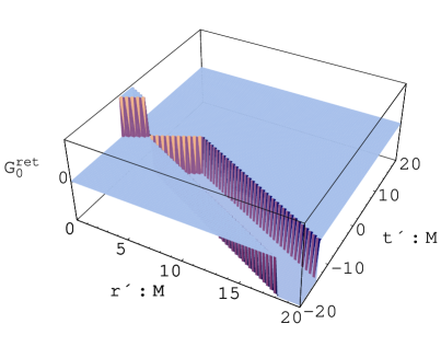
Figure 9: Flat retarded Green Function

The plots show $G_{0}(x,x^{\prime})$ for fixed $x$, where I have set $t=0,r=6M$. The values for $x^{\prime}$ range over $-20M<t^{\prime}<20M$ and $0<r^{\prime}<20M$. I have included the strip $0<r^{\prime}<2M$ in the plots to show the mathematical continuation, although the physical manifold ends at $r^{\prime}=2M$. The retarded Green function (Figure 8) is zero everywhere except on the past light cone. Interestingly it also vanishes below the past-directed light-ray that starts from $x$ and is reflected on the horizon.

The Feynman Green function (Figure 9) looks similar but further has non-vanishing support on the future light-cone (except the reflection zone).

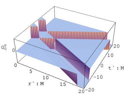
Figure 10: Flat Feynman Green Function

The support of both Green functions reaches until lightlike infinity, their amplitude remains constant, and hence causes IR divergences that are removed by the IR renormalisation.

Next I consider the symmetries of the Green functions: the Feynman Green function is symmetric in its arguments $G^{F}_{0}(x,x^{\prime})=G^{F}_{0}(x^{\prime},x)$, while the retarded Green function obeys the relation

$$G^{ret}_{0}(x^{\prime},x)=G^{ret}_{0}(x,x^{\prime})\\ -\frac{1}{2}\Big{[}\theta(r-r^{\prime}+t^{\prime}-t)-\theta(r-r^{\prime}+t-t^{\prime})+\theta(r+r^{\prime}-4M+t-t^{\prime})-\theta(r+r^{\prime}-4M+t^{\prime}-t)\Big{]}.$$ (244)

At first sight one might conclude that this difference between $G^{F}_{0}$ and $G^{ret}_{0}$ might lead to different results if employed in basic integrals, as suggested. However, an explicit calculation shows that the contribution is actually the same:

$$\int^{x}_{L}G^{F}_{0}(x,x^{\prime})F(r^{\prime})\sqrt{-g^{\prime}}dx^{\prime}\\ =\frac{1}{4}\int_{-\infty}^{t}\int_{2M}^{\infty}\Big{[}\theta(r-r^{\prime}-t+t^{\prime})-\theta(r-r^{\prime}+t-t^{\prime})\\ +\theta(r+r^{\prime}-4M+t-t^{\prime})-\theta(r+r^{\prime}-4M-t+t^{\prime})\Big{]}F(r^{\prime})dr^{\prime}dt^{\prime}\\ +\frac{1}{4}\int^{\infty}_{t}\int_{2M}^{\infty}\Big{[}\theta(r-r^{\prime}+t-t^{\prime})-\theta(r-r^{\prime}-t+t^{\prime})\\ +\theta(r+r^{\prime}-4M-t+t^{\prime})-\theta(r+r^{\prime}-4M+t-t^{\prime})\Big{]}F(r^{\prime})dr^{\prime}dt^{\prime}\\ =\frac{1}{2}\int_{-\infty}^{0}\int_{2M}^{\infty}\Big{[}\theta(r-r^{\prime}+z)-\theta(r-r^{\prime}-z)\\ +\theta(r+r^{\prime}-4M-z)-\theta(r+r^{\prime}-4M+z)\Big{]}F(r^{\prime})dr^{\prime}dz\\ =\int^{x}_{L}G^{ret}_{0}(x,x^{\prime})F(r^{\prime})\sqrt{-g^{\prime}}dx^{\prime}.$$ (245)

Indeed, if applied to basic integrals, the retarded Green function reveals the same symmetry properties as the Feynman Green function, as can be seen from (245)

$$\int_{L}G^{ret}_{0}(x,x^{\prime})F(r^{\prime})\sqrt{-g^{\prime}}d^{2}x^{\prime}=\int_{L}G^{ret}_{0}(x^{\prime},x)F(r^{\prime})\sqrt{-g^{\prime}}d^{2}x^{\prime}.$$ (246)

Further, because the perturbation series is nothing but a multiple of basic integrals (226,228) this equivalence extends to the exact Green function of the full Schwarzschild Laplacian. This means that the effective action of the dilaton model is independent of the type of Green function used. Clearly, this property already has been implied by the existence of a unique local effective action in $2d$, as discussed in Section 5.3, but by the examinations of the last Sections it can now be traced back all the way to the explicit selection of a particular Green function.

Finally I discuss the Euclidean Feynman Green function (243). The real part (Figure 10) takes exactly the same values as the original Feynman Green functions on the physical manifold (below $r=2M$ the latter is inverted).

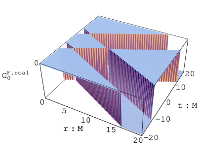
Figure 11: Euclidean Feynman Green Function, real part

This is rather surprising as it reveals some relationship between the two Feynman Green functions that is not apparent from their mathematical form. The Euclidean Feynman Green function further has an imaginary part that shows the logarithmic divergences on the light-cones which require a complicated regularisation in all explicit calculations.

The fact that the two Feynman Green functions (235,243) only differ by a divergent imaginary part suggests once more that probably something has gone wrong during the procedure of Euclideanisation. In the context of the basic integrals the imaginary part of the Euclidean Feynman Green function cannot contribute because the result shall be a real value, while the real part should give the same result as the original Feynman Green function. On the other hand one must introduce a complicated regularisation prescription, such as (237,238) (which is not unique), to handle the logarithmic divergences of the imaginary part. It is possible, and shall be shown explicitly in one case, that the renormalisation destroys the correlation with the original Green function and finally yields completely different results.

5.6 Hawking Radiation

Now all pieces are collected to calculate the complete EM tensor and, most importantly, the Hawking flux. I use the local form of the effective action (208) to calculate the basic components $\left<T\right>_{2},\left<T^{\theta}{}_{\theta}\right>_{2}$. By means of the Green function perturbation series, developed in the last Sections, I show that the basic integrals over $\square\rho\,,\,\square\phi$ indeed do not produce homogeneous solutions and therefore (208) is correct. Then I calculate the remaining components and the flux by the CF method, whereby the integration constants are chosen according to the Unruh state $\left|U\right>$. Finally I discuss how an incorrect choice of homogeneous solution leads to unphysical expectation values.

5.6.1 Expectation Values

In Section 2.4.2 I have argued that $\left<T\right>_{2},\left<T^{\theta}{}_{\theta}\right>_{2}$ are independent of the quantum state. This allows to calculate these components from the effective action which by construction leads to expectation values in the $\left|B\right>$-state. Further, they can be obtained easily by variation from (208) for $\rho$, respectively $\phi$.

In the conformal gauge the Schwarzschild metric reads $g_{\bar{\alpha}\bar{\beta}}=a_{\bar{\alpha}\bar{\beta}}e^{2\rho}$, where

$$a_{\bar{\alpha}\bar{\beta}}=\left(\begin{array}[]{cc}0&\frac{1}{2}\\ \frac{1}{2}&0\end{array}\right)\,\,,\,\,\left(a^{-1}\right)^{\bar{\alpha}\bar{\beta}}=\left(\begin{array}[]{cc}0&2\\ 2&0\end{array}\right),$$ (247)

and its inverse is $g^{\bar{\alpha}\bar{\beta}}=\left(a^{-1}\right)^{\bar{\alpha}\bar{\beta}}e^{-2\rho}$. Thus, the trace anomaly can be calculated as

$$\left<T\right>_{2}=g^{\bar{\alpha}\bar{\beta}}\frac{2}{\sqrt{-g}}\frac{\delta W}{\delta g^{\bar{\alpha}\bar{\beta}}}=\frac{2\left(a^{-1}\right)^{\bar{\alpha}\bar{\beta}}e^{-2\rho}}{\sqrt{-g}}\frac{\delta W}{\left(a^{-1}\right)^{\bar{\alpha}\bar{\beta}}(-2)e^{-2\rho}\delta\rho}\\ =-\frac{1}{\sqrt{-g}}\frac{\delta W}{\delta\rho}=-\frac{1}{12\pi}\Big{[}\square\rho+3(\nabla\phi)^{2}-2\square\phi\Big{]}.$$ (248)

Note that one has to vary not only for $\rho$ where it appears explicitly, but also where it is hidden in the metric that depends on $\rho$, as for instance in $g^{\alpha\beta}(\rho)\partial_{\alpha}\phi\partial_{\beta}\phi$. As the latter variations are traceless in $2d$, these terms do not contribute to the trace anomaly.

$\left<T^{\theta}{}_{\theta}\right>_{2}$ is given by the variation of the effective action for the dilaton field, see Section 2.2 (71). Remembering that $X=e^{-2\phi}$ we get

$$\left<T^{\theta}{}_{\theta}\right>_{2}=\frac{1}{2X\sqrt{-g}}\frac{\delta W}{\delta\phi}\\ =-\frac{1}{24\pi X}\Big{\{}2\square\rho+3(\nabla\phi)^{2}+6\nabla\rho\nabla\phi+\square\phi\bigm{[}5+6(\phi+\rho+\chi_{\phi}+\chi_{\rho})-3c_{R}\bigm{]}\Big{\}}.$$ (249)

I have given here the homogeneous solutions $\chi_{\phi},\chi_{\rho}$ of the basic integrals and the renormalisation constant $c_{R}$ to show that they appear in the same place in the expectation values. This means that if the homogeneous solutions are only constants (as I will show in the next Section), they can be absorbed by the renormalisation constant, which is then the only remaining ambiguity of the model.

In the Schwarzschild gauge the geometric fields and their derivatives are given by

$$\rho=\frac{1}{2}\ln\left(1-\frac{2M}{r}\right), \phi=-\ln r, X=r^{2}=e^{-2\phi}$$

$$(\nabla\rho)^{2}=-\frac{M^{2}}{r^{4}\left(1-\frac{2M}{r}\right)}, (\nabla\phi)^{2}=-\frac{\left(1-\frac{2M}{r}\right)}{r^{2}}, (\nabla X)^{2}=-4r^{2}\left(1-\frac{2M}{r}\right)$$

$$\square\rho=\frac{2M}{r^{3}}, \square\phi=\frac{4M-r}{r^{3}}, \square X=-2.$$

$$\nabla\rho\nabla\phi=\frac{M}{r^{3}}.$$ (250)

Inserting this into the general expressions (248,249) we obtain the expectation values in the static approximation:

$$\left<T\right>_{2} = \frac{1}{12\pi r^{2}}$$ (251)

$$\left<T^{\theta}{}_{\theta}\right>_{2} = \frac{1}{2\pi}\biggm{\{}\frac{2}{3r^{4}}-\frac{3M}{r^{5}}$$ (252)

$$+\frac{r-4M}{4r^{5}}\left[\ln\left(\frac{r-2M}{r^{3}}\right)+2(\chi_{\rho}+\chi_{\phi})-c_{R}\right]\biggm{\}}.$$

In Section 2.4.2 I have proven the state-independence of these two expectation values. Accordingly I can simply say that the system is in the $\left|U\right>$-state which is the vacuum state $\left|0\right>$. Because of the state-independence I omit the quantum state symbols.

The component $\left<T^{\theta}{}_{\theta}\right>_{2}$ shows a logarithmic divergence on the horizon. Because $\left<T^{\theta}{}_{\theta}\right>_{2}$ is invariant if we consider global coordinates this singularity is not simply a coordinate singularity. All other components of the EM tensor are regular on the horizon (in global coordinates).

5.6.2 Basic Integrals

In this Section I will show that the results obtained so far, namely the expectation values (251,252), are correct. They are based on the assumption that the homogeneous solutions $\chi_{f}$ that appear on the r.h.s. of the basic integrals (213) are only constants that do not contribute to the flux.

I start with the basic integral

$$\int_{L}G(x,x^{\prime})R(r^{\prime})\sqrt{-g^{\prime}}d^{2}x^{\prime}\\ =-\int_{L}G(x,x^{\prime})2\square^{\prime}\rho(r^{\prime})\sqrt{-g^{\prime}}d^{2}x^{\prime}=2\rho(r)+2\chi_{\rho}(r).$$ (253)

The first order approximation is obtained by replacing the full Green function by the flat one. I have already shown that the result of the perturbational analysis is independent from the choice of flat Green functions (245); in the following I will only work with the retarded Green function:

$$\int_{L}G^{ret}_{0}(x,x^{\prime})R(x^{\prime})d^{2}x^{\prime}=-2M\int_{-\infty}^{t}\biggm{[}\int_{2M}^{r-(t-t^{\prime})}\theta(r-2M-(t-t^{\prime}))\\ +\int_{2M}^{\infty}-\int_{2M}^{r+t-t^{\prime}}-\int_{4M+t-t^{\prime}-r}^{\infty}\theta(2M+t-t^{\prime}-r)-\int_{2M}^{\infty}\theta(r-2M-(t-t^{\prime}))\biggm{]}\frac{dr^{\prime}dt^{\prime}}{(r^{\prime})^{3}}\\ =2M\biggm{[}\int_{t-(r-2M)}^{t}\int_{r-(t-t^{\prime})}^{\infty}-\int_{-\infty}^{t}\int_{r+t-t^{\prime}}^{\infty}+\int_{-\infty}^{t-(r-2M)}\int_{4M+t-t^{\prime}-r}^{\infty}\biggm{]}\frac{dr^{\prime}dt^{\prime}}{(r^{\prime})^{3}}\\ =\left(1-\frac{2M}{r}\right).$$ (254)

The first order already reveals the expected properties: it is indeed independent of the time $t$ and there are no IR divergences. Clearly it vanishes for $r=2M$. The second order of the perturbation series is given by the integral $\int_{L}G^{2nd}(x,x^{\prime})R(x^{\prime})\sqrt{-g^{\prime}}d^{2}x^{\prime}$, where $G^{2nd}(x,x^{\prime})$ is (226). The first two terms can be integrated out directly like (254):

$$\frac{1}{2}\int_{L}[g(r)+g(r^{\prime})]G^{ret}_{0}(x,x^{\prime})R(x^{\prime})d^{2}x^{\prime}\\ =\frac{M}{r}\left(1-\frac{2M}{r}\right)+\frac{1}{2}\int_{L}G^{ret}_{0}(x,x^{\prime})R(x^{\prime})\frac{2M}{r^{\prime}}d^{2}x^{\prime}=\frac{1}{6}+\frac{M}{r}-\frac{8M^{2}}{3r^{2}}.$$ (255)

The third term in (226) is computed by first integrating over $x^{\prime}$:

$$\frac{1}{2}\int^{\prime\prime}G^{ret}_{0}(x,x^{\prime\prime})R(r^{\prime\prime})\int^{\prime}G^{ret}_{0}(x^{\prime\prime},x^{\prime})R(r^{\prime})d^{2}x^{\prime}d^{2}x^{\prime\prime}\\ =\frac{1}{2}\int^{\prime\prime}G^{ret}_{0}(x,x^{\prime\prime})R(r^{\prime\prime})\left(1-\frac{2M}{r^{\prime\prime}}\right)d^{2}x^{\prime\prime}=\frac{4M^{2}-6Mr+2r^{2}}{6r^{2}}.$$ (256)

The complete second order therefore reads

$$\frac{1}{2}-\frac{2M^{2}}{r^{2}}.$$ (257)

Generally, all terms in the perturbation series can be reduced to multiple integrals of the type $\int^{\prime}G(x,x^{\prime})K(r^{\prime})d^{2}x^{\prime}$, where $K(r)$ is an analytical function on $L$. In the following I summarise the integrals that appear up to the third order of the perturbation series:

$$\int^{\prime}G^{x}_{{}^{\prime}}R^{\prime} = 1-\frac{2M}{r}$$

$$\int^{\prime}G^{x}_{{}^{\prime}}R^{\prime}g^{\prime} = \frac{1}{3}-\frac{4M^{2}}{3r^{2}}$$

$$\int^{\prime}G^{x}_{{}^{\prime}}R^{\prime}(g^{\prime})^{2} = \frac{1}{6}-\frac{4M^{3}}{3r^{3}}$$

$$\int^{\prime}G^{x}_{{}^{\prime}}R^{\prime}\left(1-\frac{2M}{r}\right) = \frac{4M^{2}-6Mr+2r^{2}}{3r^{2}}$$

$$\int^{\prime}G^{x}_{{}^{\prime}}R^{\prime}g^{\prime}\left(1-\frac{2M}{r}\right) = \frac{8M^{3}-8M^{2}r+r^{3}}{6r^{3}}$$

$$\int^{\prime}G^{x}_{{}^{\prime}}R^{\prime}\left(\frac{1}{3}-\frac{4M^{2}}{3(r^{\prime})^{2}}\right) = \frac{8M^{3}-12Mr^{2}+5r^{3}}{18r^{3}}$$

$$\int^{\prime}G^{x}_{{}^{\prime}}R^{\prime}\frac{4M^{2}-6Mr^{\prime}+2(r^{\prime})^{2}}{3(r^{\prime})^{2}} = \frac{-8M^{3}+24M^{2}r-24Mr^{2}+7r^{3}}{18r^{3}}\hskip 14.22636pt$$

$$\int^{\prime}G^{x}_{{}^{\prime}}[\partial^{\prime}(g^{\prime})^{2}]\partial^{\prime}\left(1-\frac{2M}{r^{\prime}}\right) = \frac{1}{6}-\frac{4M^{3}}{3r^{3}}.$$ (258)

I have used the condensed notation $G^{x}_{{}^{\prime}}=G_{0}(x,x^{\prime})$, $G_{0}$ being either the flat retarded or the flat Feynman Green function. By (228) and this table of integrals I can calculate the third order of the perturbation series. To this approximation the considered basic integral becomes

$$\int_{L}G(x,x^{\prime})R(x^{\prime})\sqrt{-g^{\prime}}d^{2}x^{\prime}=1+\frac{1}{2}+\frac{1}{3}+\dots-\frac{2M}{r}-\frac{2M^{2}}{r^{2}}-\frac{8M^{3}}{3r^{3}}-\dots.$$ (259)

The r-dependent part equals the first terms in the power expansion of
$\ln\left(1-\frac{2M}{r}\right)$, while the constants seem to sum up to $-\ln 0$ because: $-\ln 0=\int_{0}^{1}\frac{1}{1-x}dx=\int_{0}^{1}(1+x+x^{2}+\dots)dx=1+\frac{1}{2}+\frac{1}{3}+\dots$ . Thus, I conjecture that the perturbation series of this basic integral “converges” to

$$\int_{L}G(x,x^{\prime})R(x^{\prime})\sqrt{-g^{\prime}}d^{2}x^{\prime}=\ln\frac{\left(1-\frac{2M}{r}\right)}{0}.$$ (260)

This result shows that the homogeneous solution of this basic integral is just an infinite constant $\chi_{\rho}=-\frac{1}{2}\ln 0$, because $\rho=\frac{1}{2}\ln\left(1-\frac{2M}{r}\right)$, and the integral over the full Green function acts as $-\square^{-1}$. I come back to this constant at the end of this Section.

Now I consider the second basic integral that appears in the effective action:

$$\int_{L}G(x,x^{\prime})\square^{\prime}\phi(r^{\prime})\sqrt{-g^{\prime}}d^{2}x^{\prime}=-\phi(r)-\chi_{\phi}(r).$$ (261)

$\phi=-\frac{1}{2}\ln X=-\ln r$ was the “re-defined” dilaton field and $\square\phi=\frac{4M-r}{r^{3}}$. The first order of the perturbation series now gives

$$\int_{L}G_{0}(x,x^{\prime})\frac{4M-r^{\prime}}{(r^{\prime})^{3}}d^{2}x^{\prime}\approx-\left(1-\frac{2M}{r}\right)+\ln\left(\frac{r}{2M}\right).$$ (262)

The first two terms of the second order (226) are

$$\frac{M}{r}\left[-\left(1-\frac{2M}{r}\right)+\ln\left(\frac{r}{2M}\right)\right]+\frac{1}{12}\left(1-\frac{2M}{r}\right)\left(1-\frac{4M}{r}\right),$$ (263)

while the third term results in

$$\frac{3}{4}\left(1-\frac{2M}{r}\right)-\frac{M}{r}\ln\left(\frac{r}{2M}\right).$$ (264)

Hence, the considered basic integral up to the second order perturbation theory reads

$$\int_{L}G_{0}(x,x^{\prime})\frac{4M-r^{\prime}}{(r^{\prime})^{3}}d^{2}x^{\prime}=\ln\left(\frac{r}{2M}\right)-\left(1-\frac{2M}{r}\right)\left(\frac{1}{6}+\frac{4M}{3r}\right).$$ (265)

This shows that the leading order, up to a constant $-\ln 2M$, is $\ln r$. Hence, again the homogeneous solution can only be a constant $\chi_{\phi}=\ln 2M$. I conjecture that the remaining orders of the perturbation series slowly decrease the superfluous higher orders in $r$. But, as already concluded before in Section 5.3, the leading order is sufficient to determine the homogeneous solution, therefore the latter must be $r$-independent.

I have shown now that for both basic integrals appearing in the non-local form of the effective action (207), the homogeneous solutions are just constants:

$$\int_{L}G(x,x^{\prime})R(r^{\prime})d^{2}x^{\prime} = 2\rho(r)-\ln 0$$ (266)

$$\int_{L}G(x,x^{\prime})\square\phi(r^{\prime})d^{2}x^{\prime} = -\phi(r)-\ln 2M.$$ (267)

These results differ only by the constants from the ones obtained by setting $\square^{-1}\square=1$, see Section 5.3. They are a direct consequence of the boundary condition that the Green functions vanish on the horizon and guarantee that the basic integral vanish for $r=2M$. Hence, by including these boundary conditions, one has

$$\square^{-1}\square f(r)=f(r)-f(2M).$$ (268)

From equation (211) the appearance of these constants was not apparent, at first sight. They are absent, because at that point I had only adapted the Green functions to the half-plane. Consequently one must also adapt the delta-function to the half-plane. If it is decomposed into eigenfunctions it adopts their boundary conditions, namely that they vanish at the horizon. An easier way is to guess the correct delta-function. Just like the Green functions it can be constructed by substracting from the original one the mirrored delta-function on the horizon:

$$\delta_{hp}(x-x^{\prime}):=\delta(r-r^{\prime})\delta(t-t^{\prime})-\delta(r+r^{\prime}-4M)\delta(t-t^{\prime}).$$ (269)

For $r>2M\vee r^{\prime}>2M$ the mirrored part does not contribute, because then the condition $r=4M-r^{\prime}$ cannot be fulfilled. For $r=2M$ or $r^{\prime}=2M$ the delta-function vanishes. Going back to Green’s theorem (210) and inserting $\square^{x^{\prime}}G(x,x^{\prime})=-\delta_{hp}(x-x^{\prime})$ instead of $\square^{x^{\prime}}G(x,x^{\prime})=-\delta(x-x^{\prime})$ we obtain the same relation as before (211) where $f(x)$ is replaced by $f(r)-f(2M)$. Note that throughout the derivation of the Green function perturbation theory I have used the ordinary delta-function of the full-plane. The delta-function only appears in the perturbation series where a flat Laplacian $\square_{0}$ is separated from the perturbing Laplacian $\delta\square$. As $\delta\square$ is always accompanied by an integration over the variable on which it acts and the integrand contains a flat Green function with the same argument, the mirrored part of the delta-function cannot lead to contributions because the Green function vanishes at the horizon!

Finally, by the modification of the delta-function according to (269) the picture is complete: the Green function perturbation theory on the half-plane equipped with the boundary conditions of Section 5.3 is now fully self-consistent and yields the expected results, up to constants.
It remains to examine if and how these constants affect the expectation values. The effective action is simply changed by replacing $\rho\to\rho+\chi_{\rho}$ and $\phi\to\phi+\chi_{\phi}$. From (208) and the expectation values (248,249) we see that only $\left<T^{\theta}{}_{\theta}\right>_{2}$ acquires an additional term

$$\left<T^{\theta}{}_{\theta}\right>_{2}=\text{old}+\frac{r-4M}{4\pi r^{5}}(\chi_{\rho}+\chi_{\phi}).$$ (270)

Interestingly, the Hawking flux, given by the component $\left<T^{r}{}_{t}\right>$ of the EM tensor, remains the same. This can be seen by the integral over $\left<T^{\theta}{}_{\theta}\right>_{2}$ that determines the constant $K$ in the CF approach, see Section 2.4.1:

$$K\propto\int_{2M}^{\infty}(r^{\prime}-2M)\left<T^{\theta}{}_{\theta}\right>_{2}dr^{\prime}=\text{old}+(\chi_{\rho}+\chi_{\phi})\int_{2M}^{\infty}\frac{(r^{\prime}-2M)(r^{\prime}-4M)}{4\pi(r^{\prime})^{5}}dr^{\prime}\\ =\text{old}+0.$$ (271)

Accordingly, the asymptotic energy density and asymptotic radial stress are unaffected by the constants. Note that the flux is unaffected everywhere, not only asymptotically, because it only contains an $r^{-2}$-term (in the static approximation). However, energy density and stresses for finite radius $r$ do depend on them.

The actual values of the constants $\chi_{\rho},\chi_{\phi}$ are a direct consequence of the boundary condition at $r=2M$ as they only shift the absolute value of the basic integrals to the correct position. It is rather obvious that a different boundary condition on the horizon only changes the values of the constants in a way that they shift the r.h.s. of (211) in agreement with the l.h.s., i.e. the value of the basic integral on the horizon. If this assumption is correct, the Hawking flux is independent of the boundary conditions imposed at the horizon. A crucial role is certainly played by the IR renormalisation that in my approach enters as a boundary condition at infinity.

I have already observed that (252) and thus all expectation values of the EM tensor have the same dependence on the homogeneous solutions as on the renormalisation constant $c_{R}$. The remaining ambiguity of the EM tensor (if the quantum state has already been fixed) can therefore be put into this single constant.

Remark: Until now I have only considered the flat Green functions derived directly in Minkowski spacetime to evaluate the basic integrals via the perturbation theory. Because the Euclidean Feynman Green function (237) is often employed in two-dimensional problems, it is interesting whether it reproduces the obtained results of the perturbational analysis. Clearly it must fulfil the required boundary conditions. The Euclidean Green function on the half-plane (243) vanishes at the horizon, i.e. for $r=2M$ or $r^{\prime}=2M$. The IR renormalisation is no more carried out by dropping boundary terms, but by using the regularised version of the Euclidean Feynman Green function (238). On the half-plane again the mirrored term will be added. I assume that the series converges and that the first order term gives the leading order in $r$ for $r\to\infty$. The basic integral with the scalar curvature $R$ is then approximated by

$$\lim_{\lambda\to 0}\frac{d}{d\lambda}\biggm{\{}\lambda\frac{2M\,i}{\pi}\frac{\Gamma\left(-\frac{\lambda}{2}\right)}{\Gamma\left(1+\frac{\lambda}{2}\right)2^{1+\lambda}}\\ \int_{L}\frac{[(t-t^{\prime})^{2}-(r-r^{\prime})^{2}]^{\frac{\lambda}{2}}-[(t-t^{\prime})^{2}-(r+r^{\prime}-4M)^{2}]^{\frac{\lambda}{2}}}{(r^{\prime})^{3}}d^{2}x^{\prime}\biggm{\}}.$$ (272)

The integration over $t^{\prime}$ gives

$$\int_{-\infty}^{\infty}\left\{[(t-t^{\prime})^{2}-(r-r^{\prime})^{2}]^{\frac{\lambda}{2}}-[(t-t^{\prime})^{2}-(r+r^{\prime}-4M)^{2}]^{\frac{\lambda}{2}}\right\}dt^{\prime}\\ =\sqrt{\pi}(-1)^{\frac{\lambda+1}{2}}\frac{\Gamma\left(-\frac{\lambda+1}{2}\right)}{\Gamma\left(-\frac{\lambda}{2}\right)}\left\{\left[(r-r^{\prime})^{2}\right]^{\frac{\lambda+1}{2}}-\left[(r+r^{\prime}-4M)^{2}\right]^{\frac{\lambda+1}{2}}\right\}.$$ (273)

As I am interested in the asymptotic behaviour ($r\to\infty$) of the basic integral I can facilitate the integration over $r^{\prime}$ by assuming that $r>r^{\prime}$ and therefore $\left[(r-r^{\prime})^{2}\right]^{\frac{\lambda+1}{2}}=(r-r^{\prime})^{\lambda+1}$ and $\left[(r+r^{\prime}-4M)^{2}\right]^{\frac{\lambda+1}{2}}=(r+r^{\prime}-4M)^{\lambda+1}$. The integral over $r^{\prime}$ from $2M$ to $\infty$ can then be performed analytically and yields a hypergeometric function:

$$\int_{2M}^{\infty}\frac{(r-r^{\prime})^{\lambda+1}-(r+r^{\prime}-4M)^{\lambda+1}}{(r^{\prime})^{3}}dr^{\prime}\\ =\frac{(2M)^{\lambda-1}}{\lambda-1}\biggm{\{}(-1)^{\lambda}F\left[-1-\lambda,1-\lambda,2-\lambda,\frac{r}{2M}\right]\\ +F\left[-1-\lambda,1-\lambda,2-\lambda,2-\frac{r}{2M}\right]\biggm{\}}.$$ (274)

Now it is a simple task to carry out the renormalisation procedure to obtain the first order of the basic integral:

$$\int_{L}G_{F}^{mod}(x,x^{\prime})R(x^{\prime})\sqrt{-g^{\prime}}d^{2}x^{\prime}\stackrel{{\scriptstyle r\to\infty}}{{\to}}\lim_{\lambda\to 0}\frac{d}{d\lambda}\biggm{\{}\frac{\lambda}{\lambda-1}\frac{i\,M^{\lambda}(-1)^{\frac{\lambda+1}{2}}}{2\sqrt{\pi}}\frac{\Gamma\left(-\frac{\lambda+1}{2}\right)}{\Gamma\left(1+\frac{\lambda}{2}\right)}\\ \biggm{(}(-1)^{\lambda}F\left[-1-\lambda,1-\lambda,2-\lambda,\frac{r}{2M}\right]+F\left[-1-\lambda,1-\lambda,2-\lambda,2-\frac{r}{2M}\right]\biggm{)}\biggm{\}}\\ =\frac{r}{2M}-1.$$ (275)

This result is obviously not in agreement with the one obtained by the original Feynman Green function. By (213,214) and $R=-2\square\rho$ I see that the homogeneous solution associated to $\rho$ must be

$$\chi_{\rho}=\frac{1}{2}\left(\frac{r_{\ast}}{2M}-1-\ln 0\right),$$ (276)

i.e. $C_{1}^{\rho}=-\frac{1}{2}-\ln 0\,,\,C_{2}^{\rho}=\frac{1}{2}$, and the exact basic integral is

$$\int_{L}G_{F}^{mod}(x,x^{\prime})\square^{\prime}\rho(x^{\prime})\sqrt{-g^{\prime}}d^{2}x^{\prime}=-(\rho+\chi_{\rho})\\ =\frac{1}{2}+\ln 0-\frac{r}{4M}-\frac{1}{2}\ln\left[\biggm{(}1-\frac{2M}{r}\biggm{)}\biggm{(}\frac{r}{2M}-1\biggm{)}\right].$$ (277)

If the perturbation theory works correctly with the Euclidean Feynman Green function it should produce the asymptotic expansion of the logarithmic term at the higher orders. Anyway, this result is in conflict with the one obtained by the original Green functions and also with the considerations on the boundary conditions in Section 5.3. There I have shown that the homogeneous solution only can be a constant if the boundary terms in (211) vanish through the elimination of IR divergences.

That the boundary terms vanish, in particular those at infinity, was one of my basic assumptions, inspired by physical arguments. If this is correct, the usage of the Euclidean Feynman Green function leads to an inconsistency, namely the r.h.s. of (211) is still $-f$, while the l.h.s. produces an additional homogeneous solution like $\chi_{\rho}$ above.

5.6.3 Hawking Flux and Energy Density

With the computation of the components $\left<T\right>_{2}$ and $\left<T^{\theta}{}_{\theta}\right>_{2}$ most of the work is done to determine the vacuum expectation value of the complete EM tensor. It remains to calculate the constant $K$ of the CF approach for the Unruh state $\left|U\right>$ which has been identified with the vacuum state of the model (see Section 2.4.1). Remember that the other constant $Q$ was set to zero for all physical states. In the Unruh state we have the relation $K_{U}=\frac{M^{2}f(\infty)}{2}$ (see Table 2 at the end of Section 2.4.1) where $f(r)$ is the state-independent function (92):

$$K_{U}=\frac{M^{2}}{2}\int_{2M}^{\infty}\left[\frac{\left<T\right>_{2}M}{(r^{\prime})^{2}}+2(r^{\prime}-2M)\left<T^{\theta}{}_{\theta}\right>_{2}\right]dr^{\prime}=-\frac{1}{768\pi}.$$ (278)

By the CF equations (78,79) the total flux through a spherical shell surrounding the BH is then given by [5]

$$\text{Flux}_{tot}=\left<U\left|T^{r}{}_{t}\right|U\right>_{2}=-\frac{K}{M^{2}}=\frac{1}{768\pi M^{2}},$$ (279)

and the measurable four-dimensional flux is (see (68))

$$\left<U\left|T^{r}{}_{t}\right|U\right>=\frac{1}{3072\pi^{2}M^{2}r^{2}}.$$ (280)

Hence it is by a factor $40$ larger than the total flux calculated by the Black Body hypothesis (27) which for a “minimal” effective area $A=16\pi M^{2}$ is the widely accepted result. It might well be that a quantum calculation directly in four dimensions could reproduce the correct flux for the Black Body law; in this case the deviation between (280) and (27) would indicate the failure of the dilaton model at the quantum level to describe a spherically symmetric four-dimensional theory. On the other hand, it is questionable if the Black Body hypothesis alone is sufficient to determine the Hawking flux as it is based on a semi-classical calculation and an assumption concerning the effective area; the cross section of particles without self-interaction on a Schwarzschild background involves only free propagators and no loop-graphs. In contrast to that the current approach includes the full quantum theory of free scalar particles which is provided by the one-loop order. Such a calculation clearly describes the processes near the horizon that occur in QFT. By this reasoning (280) could instead be closer to the correct value of the Hawking flux.

Although the results obtained here may not be the final answer, they reveal some nice qualitative features which are in agreement with the expected properties of BH radiation. First of all, the flux as well as the energy density (see below) do not violate the weak energy condition in the asymptotic Minkowski region of spacetime. I emphasize this seemingly trivial point, because there has been lots of confusion during the last years in the literature, where exactly this happened by wrong calculations and it was interpreted as a principle failure of the dilaton model. Interestingly, (280) is identical to the result for the intrinsic two-dimensional model [5].

Finally, I present the vacuum expectation values of the remaining components of the EM tensor in the Schwarzschild gauge. The energy density is given by

$$\left<T_{tt}\right>_{2}=\frac{1}{768\pi M^{2}}+\frac{7}{24\pi r^{2}}-\frac{7M}{6\pi r^{3}}+\frac{9M^{2}}{8\pi r^{4}}\\ +\frac{\left(1-\frac{2M}{r}\right)^{2}\left[\ln\frac{r-2M}{r^{3}}+2(\chi_{\rho}+\chi_{\phi})-c_{R}\right]}{8\pi r^{2}}$$ (281)

and the radiational stress can be calculated by $\left<T_{rr}\right>_{2}=g_{rr}(\left<T\right>_{2}-\left<T^{t}{}_{t}\right>_{2})$. Again, the four-dimensional components can be reconstructed by (68). Note that the logarithmic term in the energy density brings in a further mass-dependence as compared to the case of massive particles (183). In particular, this means that the point where the energy density changes sign now depends on the BH mass. Figures 12,13,14 show the energy density for two BHs whose mass is one time much larger than the Planck mass and the other time much smaller. For a very small BH $M=10^{-20}$ the point of sign-reversal lies exactly on the horizon.

Figure 12: Small Black Hole, $M=10^{-20}$

For huge BHs $M=10^{40}$ this point is shifted far away from the horizon (Figure 13).

Figure 13: Large Black Hole, $M=10^{40}$

Note that for masses smaller than the Planck mass $M<1$ the results loose their significance because the BH is then in a rapidly evolving state where backreaction effects play an important role. With respect to this, Figure 12 cannot be taken too seriously (although it shows that the zone of negative energy density decreases with the BH mass). Figure 14 shows the energy density for a BH of the same size but close to the horizon.

Figure 14: Large Black Hole, $M=10^{40}$

Surprisingly, the event horizon is surrounded by a large zone of negative energy density, caused by the virtual particles that are swallowed by the BH and thereby decrease its mass. Such an effect already has been observed for massive particles, see Figure 6. There I argued that for fixed BH mass this zone decreases with the rest mass of the emitted particles. This idea is in agreement with the current results, because it states that particles with higher kinetic energy can be produced closer to the horizon, as they have a higher probability to leave the BH. As the Hawking temperature, and hence the energy of massless scalar particles, becomes higher with decreasing BH mass, the point of production accordingly approaches the horizon.

Remark: It is now a trivial task to calculate the components of the EM tensor in the Hartle-Hawking state $\left|H\right>$. The total flux is just zero, as $K$ is set to zero, and the asymptotic energy density is by a factor $2$ larger than in the $\left|U\right>$-state. All higher orders in $r$ of the energy density are identical in the two states.

Further Remark: In the last Section I have shown that the homogeneous solutions $\chi_{\rho},\chi_{\phi}$ are constants and therefore do not affect the Hawking flux. If, for some reason, one uses an r-dependent homogeneous solution (like e.g. the one obtained for the Euclidean Feynman Green function (276)) the flux and other components of the EM tensor are changed. For instance, I will assume that

$$\chi_{\rho}^{new}=\frac{1}{2}\left[\frac{r}{2M}+\ln\left(\frac{r}{2M}-1\right)-1-\ln 0\right],$$ (282)

and $\chi_{\phi}=\ln 2M$ as before. This means that the first basic integral would give the result

$$\int_{L}G(x,x^{\prime})R(r^{\prime})d^{2}x^{\prime}=\frac{r}{2M}+\ln\left[\biggm{(}\frac{r}{2M}-1\biggm{)}\biggm{(}1-\frac{2M}{r}\biggm{)}\right]-1-2\ln 0.$$ (283)

This choice is compatible with the boundary condition for the Green function at the horizon (the basic integral vanishes for $r=2M$), but not with the ones at infinity. Namely, as discussed in Section 5.3 and Section 5.6.2, if the Green functions vanish asymptotically (or merely are set to zero by an IR renormalisation) the homogeneous solutions are constants that are unambiguously fixed by the boundary condition at the horizon. If for some reason they are nontrivial functions in $r$ (e.g. by using the Euclidean Feynman Green function) one must reconsider the problem of IR renormalisation to compute the correct boundary terms that restore consistency in (211).

In the $\left|U\right>$-state the flux-determining constant $K$ acquires an additional contribution, such that

$$K_{U}^{new}=\text{old}+M^{2}\int_{2M}^{\infty}\frac{(r^{\prime}-2M)(r^{\prime}-4M)}{4\pi(r^{\prime})^{5}}\chi_{\rho}^{new}dr^{\prime}=\text{old}+\frac{1}{128\pi}=\frac{5}{768\pi}.$$ (284)

As a consequence, the flux as well as the asymptotic energy density become negative which means that the weak energy condition is violated in the flat (asymptotic) region! From the physical point of view this result is nonsense and demonstrates the importance of a consistent IR renormalisation. The same result (284) was obtained by Balbinot-Fabbri [31], Equation 16.

5.7 Quantum States and the Effective Action

Concerning the relation between the effective action and the choice of quantum state, there have been two basic assumptions which are the very basis of the computations in my thesis:

• First of all, I have assumed that the effective action does not produce quantum mechanical expectation values in the $\left|U\right>$-state (which is the vacuum state of the system), hence the components of the EM tensor cannot be derived directly from the effective action.

• Second, I have assumed (and proven by heuristic arguments in Section 2.4.2) that the basic components of the CF approach, $\left<T\right>$ and $\left<T^{\theta}{}_{\theta}\right>$, are independent of the quantum state and therefore nevertheless can be derived directly from the effective action.

In the present Section I will reconsider these assumptions by explicitly calculating the remaining components of the EM tensor (apart from the basic ones) by variation of the effective action (208):

$$\left<T_{\alpha\beta}\right>_{2}=\frac{2}{\sqrt{-g}}\frac{\delta W}{\delta g^{\mu\nu}}\\ =\frac{1}{12\pi}\biggm{\{}\Bigm{[}\partial_{\alpha}\phi\partial_{\beta}\phi-\frac{g_{\alpha\beta}}{2}(\partial\phi)^{2}\Bigm{]}\Bigm{[}5+6(\phi+\chi_{\phi}+\rho+\chi_{\rho})-3c_{R}\Bigm{]}\\ -\Bigm{[}\partial_{\alpha}\rho\partial_{\beta}\rho-\frac{g_{\alpha\beta}}{2}(\partial\rho)^{2}\Bigm{]}+4\Bigm{[}\partial_{\alpha}\phi\partial_{\beta}\rho-\frac{g_{\alpha\beta}}{2}(\partial_{\gamma}\phi)(\partial^{\gamma}\rho)\Bigm{]}\biggm{\}}+\frac{2}{\sqrt{-g}}\frac{\delta W}{\delta\rho}\frac{d\rho}{dg^{\alpha\beta}}.$$ (285)

To compute the last term I need the definition of the conformal metric, see Appendix A.3. Its determinant is related to $\rho$ by $g=\det(g_{\bar{\alpha}\bar{\beta}})=-\frac{e^{4\rho}}{4}$ or $\sqrt{-g}=\frac{e^{2\rho}}{2}$, hence $\frac{d\sqrt{-g}}{d\rho}=2\sqrt{-g}$. Using further the relation $\frac{d\sqrt{-g}}{dg^{\alpha\beta}}=-\frac{\sqrt{-g}}{2}\cdot g_{\alpha\beta}$ I can calculate this term to

$$\frac{2}{\sqrt{-g}}\frac{\delta W}{\delta\rho}\frac{d\rho}{dg^{\alpha\beta}}=\frac{g_{\alpha\beta}}{24\pi r^{2}}.$$ (286)

If contracted by the metric it gives the correct trace anomaly, all other terms in (285) are traceless.

The first thing I observe is that the flux component of the EM tensor now indeed vanishes:

$$\left<T^{r}{}_{t}\right>_{2}=0\Bigm{(}=\left<H\left|T^{r}{}_{t}\right|H\right>_{2}=\left<B\left|T^{r}{}_{t}\right|B\right>_{2}\Bigm{)}.$$ (287)

This is a direct consequence of the static approximation because the Schwarzschild metric has no off-diagonal entries $g_{rt}=0$. This proves the assumption that the expectation values derived from the effective action are not the ones in the $\left|U\right>$-state because there we have a finite flux. Next I consider the energy density which becomes

$$\left<T_{tt}\right>_{2}=\frac{1}{4\pi r^{2}}-\frac{13M}{12\pi r^{3}}+\frac{9M^{2}}{8\pi r^{4}}\\ +\frac{\left(1-\frac{2M}{r}\right)^{2}\left[\ln\frac{r-2M}{r^{3}}+2(\chi_{\rho}+\chi_{\phi})-c_{R}\right]}{8\pi r^{2}}.$$ (288)

If I compare this result with the energy density in the Unruh state (281) I see that it differs from it by $\frac{1}{768\pi M^{2}}+\frac{1}{24\pi r^{2}}\left(1-\frac{2M}{r}\right)$. The leading order (which is constant in $2d$) corresponds to the occupied real particle states. Thus, the state of the effective action can be identified with the Boulware state $\left|B\right>$ (see Section 2.4.1) as it is the only state which contains no radiative components of the EM tensor, i.e. the spacetime is asymptotically vacuum (in the Hartle-Hawking state $\left|H\right>$ the asymptotic energy density is twice the one in the Unruh state). In the CF approach the Boulware state is reached by fixing the constants $K_{B}=0$ as $Q_{B}=\frac{1}{384\pi}$ (remember that the choice $Q\neq 0$ produces a quadratic divergence of the EM tensor on the horizon in global coordinates, hence $\left|B\right>$ has no physical significance); note that the energy density calculated a la CF still differs from (288) by a term $\frac{1}{24\pi r^{2}}\left(1-\frac{2M}{r}\right)$!

This result can be understood by reconsidering the static approximation. If any radiation components are present (let’s say in the stationary $\left|H\right>$-state) one must observe inevitably occupied states in the asymptotic region and a non-zero spacetime curvature at some time-slice. If the spacetime is assumed to be static this asymptotic spacetime curvature is always present. Hence, the asymptotically flat Schwarzschild geometry can only describe correctly a quantum state in the static approximation with no occupied particle states in the asymptotic region, i.e. $\left|B\right>$. If one wanted to construct an effective action that yields expectation values e.g. in the $\left|H\right>$-state one had to construct a complicated geometry capable to describe the asymptotic region. Clearly, this problem is created by the static approximation as it continues the actual spacetime geometry into the remote past and future. In the quasi-static phase a BH spacetime (or better space) is indeed best described by the Schwarzschild geometry, but by infinitely extending it one must either take into account the occupied asymptotic states or creates the divergence on the horizon of the Boulware state.

This result is not at all disappointing as it has been proven by Wald [32, 33] that the expectation value of the EM tensor is unique up to a generally conserved expression (in the dilaton model this expression fulfils the non-conservation equation). The CF approach shows explicitly how one can switch between representations of the EM tensor (corresponding to different quantum states) by simply adding a covariantly conserved expression of the form

$$\Delta\left<T^{\mu}{}_{\nu}\right>=\large\frac{1}{M^{2}}\left(\begin{array}[]{cc}\frac{\Delta K_{2}-\Delta Q_{2}}{\left(1-\frac{2M}{r}\right)}&\frac{\Delta K_{2}}{\left(1-\frac{2M}{r}\right)^{2}}\\ -\Delta K_{2}&\frac{\Delta Q_{2}-\Delta K_{2}}{\left(1-\frac{2M}{r}\right)}\end{array}\right).\normalsize$$ (289)

By these considerations I can summarise and answer the problem of the effective action and its expectation values by some unexpected but nice statements:

• The effective action yields only expectation values in the unphysical, but the conservation equation satisfying, Boulware state.

• The Unruh state (which is the vacuum state of the model) as well as the Hartle-Hawking state, leading both to the same outgoing Hawking flux, can be adjusted by adding an expression (289) with the appropriate choice of the constants $\Delta K_{2},\Delta Q_{2}$.

• The desired quantum state cannot be fixed directly in the effective action by the choice of Green function, as supposed, neither by the fixation of the renormalisation ambiguity. The quantum state of the effective action originates from the geometry of the static approximation.

These points have often caused confusion in the literature. It has been stated [31] that the logarithmic divergence of the $T^{\theta}{}_{\theta}$-component (252) shows that it corresponds to the Boulware state, and it was claimed that the same component in the Unruh state would be finite at the horizon.

In Section 2.4 I have demonstrated how a quadratic divergence in the radiation components of the EM tensor (not in $T^{\theta}{}_{\theta}$) can be removed by adjusting the constant $Q$. Any other divergences that enter by the basic functions cannot be removed and are thus state-independent. Further, I have shown in the current Chapter that the logarithmic divergence found in $T^{\theta}{}_{\theta}$ is a direct consequence of the IR renormalisation that fixes the homogeneous solutions in the basic integrals (211). Because of these arguments I have very good reasons to contradict the authors of [31].

6 Conclusions

The aim of my thesis was to calculate quantum mechanical expectation values of a scalar field on a Schwarzschild spacetime whose mass $M$ was assumed to be sufficiently large so that the spacetime could be considered as static. I could show, developing further previous work, that this can be done for massive particles directly in $4d$, and for massless particles in the two-dimensional dilaton model. In the following, I will sketch the considerations and calculations which led to these results in a chronological order.

One of the basic tools of this work was the CF method [1]. It allows to calculate the complete EM tensor on a Schwarzschild spacetime from two “basic components” $T,T^{\theta}{}_{\theta}$ and two integration constants $K,Q$ by the conservation equation (11). The EM tensor is thereby restricted by the spherical symmetry conditions which means singling out the s-modes of the scalar field, and thus has the form (55) at the classical and quantum level. Because I applied the method to expectation values I had to show that the conservation equation still holds for the renormalised expectation value of the EM tensor (47). Further, I could verify that also the non-conservation equation of the dilaton model survives the quantisation procedure (87).

The problem of the boundary conditions and the quantum state appeared throughout this thesis. The first observation was that the classical solution of the scalar field $S_{0}$, which is always added to the quantum fluctuations and enters the path integral, is most conveniently set to zero (see Section 1.2.1). In particular, this choice was in agreement with the representation of the effective action as a functional determinant (97) which demanded the vanishing of a boundary term. In Section 2.4 I considered three different quantum states that correspond to different choices of the constants $K,Q$ (see Table 2 at the end of Section 2.4.1). Following [1] I could verify that the condition $Q=0$ guarantees the regularity of the EM tensor in global coordinates and hence singles out the physical states. The remaining constant $K$ was shown to regulate the incoming flux and thus the number of occupied states at past null infinity ${\cal I}^{-}$ (Figure 1). The outgoing flux turned out to be independent of $K$. I identified the Unruh state $\left|U\right>$ with the vacuum state of the theory as it led to the minimal energy density of the physical states (see Figure 4). Further, I considered the Boulware state $\left|B\right>$: because of $Q_{B}\neq 0$ it does not belong to the physical states. However, as it is characterised by vanishing asymptotic fluxes I could identify it with the state of the effective action. In Section 5.7 I demonstrated by direct calculation that the effective action indeed leads to expectation values in the $\left|B\right>$-state. I interpreted this result in the following way: the effective action yields expectation values in the form of geometric objects, such as the scalar curvature. In the static approximation the asymptotic state must be the vacuum state, i.e. there cannot be occupied particle states in the asymptotic region. This is only fulfilled by the $\left|B\right>$-state which is therefore the only state in accord with the static approximation. Nevertheless, it was still possible to compute expectation values in arbitrary quantum states. Namely, I used the effective action only for the computation of the basic components, whereby the crucial point was to show the state-independence of the latter in Section 2.4.2. The physical argument was that the basic components did not correspond to radiational degrees of freedom. The remaining components were calculated a la CF anyway, so the state was finally fixed by the constants $K,Q$ alone.

The next task was to establish the effective action. In a first step I used the zeta-function regularisation (103,104) to express the effective action in terms of the heat kernel (107,108). Then I distinguished between massive and massless scalar fields: in the massive case I could find a local form of the heat kernel by the Seeley-DeWitt expansion (111) whose convergence was guaranteed by the mass term (for sufficiently large particle mass $m$). In Section 3.1.3 I examined the general conditions for the convergence of the local expansion in the presence of a damping term in the classical action. In the massless case I derived a non-local effective action (142) by the covariant perturbation theory invented by Barvinsky and Vilkovisky [4, 26].

The treatment of massive particles was straightforward: I calculated the basic components by the effective action and used the CF approach to obtain the remaining components like the energy density and the flux. I renormalised the effective action by substracting the flat spacetime values of the expectation values and by setting the remaining renormalisation constant $c_{ren}$ to zero so that the expectation value of the EM tensor vanishes (in the Unruh state) if the particle mass $m$ goes to infinity. For fixed $m$ the obtained energy density revealed the expected behaviour (Figure 6): near the horizon it is negative by the presence of virtual particles with negative flux that fall into the BH. Then it becomes positive for $r\approx 2.75M$ and falls off like $r^{-2}$ in the asymptotic region (183) (i.e. a spherical shell has constant energy, corresponding to the occupied states). The result for the local flux was (182). Near the critical point of the Seeley-DeWitt expansion $\alpha=(mM)^{-1}\approx 1$ the agreement with the Black Body law for massive particles (188) and the result for massless particles (280) (which should be some orders beyond) was reasonable (though at this point the perturbation series actually diverges). However, in the convergence region $\alpha\ll 1$ the quantum calculation could not reproduce the expected exponential damping as illustrated in Table 6. The reason was that the convergence condition $\alpha\ll 1$ of the perturbation series automatically restricted the scope of the analysis to the region where the exponential damping already had set in and thereby practically eliminated the contribution of the massive particles. For a correct description in the interesting range $\alpha\approx 1$ the usage of a non-local effective action therefore seems to be unavoidable (see in the Outlook). From the phenomenological point of view such an investigation could be of interest as there is sufficient freedom to adjust the BH mass $1\ll M<10^{20}$ such that the BH is still in the quasi-static phase and the particle mass is within the range of the fundamental particles $m\approx M^{-1}$.

The examinations of massless particles in the two-dimensional dilaton model has been the main concern of my thesis. First of all, I could establish a non-local effective action by the covariant perturbation theory including a non-trivial endomorphism. This was a nice result, even more as Barvinsky and Vilkovisky [4, 26] themselves claimed that the case of a conformally coupled scalar field would represent the only possible application of their formalism in two dimensions! Furthermore, the effective action up to now had only been derived by integration of expectation values [5], such as the trace anomaly, and not directly from the Euclidean path integral. Therefore, the construction of the effective action (208) by the method of Barvinsky and Vilkovisky can be seen as a missing link in the current literature which I have supplemented in my thesis. Another point which was widely discussed have been the boundary conditions and their connection to the quantum state. My first observation was that the quantum state of the effective action is fixed by the homogeneous solution that emerges through the non-local expression $\square^{-1}$. Because of the integrability of two-dimensional gravity the explicit knowledge of the Green functions of the two-dimensional Schwarzschild Laplacian was not necessary to compute the effective action. Therefore, the behaviour of the Green functions on the boundary, including the event horizon $r=2M$, was sufficient to determine uniquely the quantum state of the effective action which could then be given in a local form. In Section 5.3 I argued that the IR renormalisation suggests a vanishing of the Green functions at the boundary which fixes the homogeneous solutions (as constants) by the prescription $\square^{-1}\square=1$ (211).

Beyond that, I investigated the two-dimensional Green functions by a perturbation series (216). I could show that the series converges if

• The analysis is restricted to the half-plane $2M<r<\infty$ (which is sensible as the flux is produced outside the horizon).

• The boundary conditions are imposed according to the IR renormalisation.

• The Green functions are applied to basic integrals (213).

As starting point of the perturbation series I chose the flat retarded (232) and Feynman (235) Green function on the half-plane which I calculated by Fourier transformation without Euclideanizing spacetime. The explicit evaluations with the Green functions proved consistency with the considerations on the boundary terms in Section 5.3, whereby the boundary condition at the horizon fixed the constant homogeneous solutions. The latter could be shown to leave the Hawking flux invariant (271).

The result for the Hawking flux agreed with the one already obtained in [5]. The progresses achieved in my thesis were on the one hand the direct derivation of the effective action from the heat kernel and on the other hand the explicit examination of boundary terms and their effect on the expectation values of the EM tensor. The energy density (281) which I calculated a la CF (like the flux) revealed a similar behaviour like the one in the massive case. It is characterised by the existence of a zone of negative energy density which in the massless case turned out to be scale-dependent (Figures 12,13,14).

Finally, I concluded that the quantum state of the effective action is indeed the Boulware state as it produces an EM tensor that in the CF approach corresponds to the choice $Q=K=0$. Nevertheless, all quantum states of the expectation values are accessible by adding a covariantly conserved EM tensor of the type (289), the basis of this method being the state-independence of the basic components $\left<T\right>,\left<T^{\theta}{}_{\theta}\right>$.

7 Outlook

The examinations of my thesis can be continued and supplemented into various directions. I give a list of some of them, whereby I quote those first which are a direct extension of this work.

The investigations of the massive particles by the local Seeley-DeWitt expansion of the heat kernel in four dimensions have shown that the interesting range of the parameters in the static approximation $M>1,m\approx M^{-1}$ lies beyond the scope of the local expansion. This suggests to consider massive particles in the two-dimensional dilaton model, where one can work easily with the non-local effective action of the covariant perturbation theory (142). The mass term modifies the two-dimensional Laplacian by a term $X\cdot m^{2}$, $X$ being the dilaton field. Now one can either keep this term as an endomorphism $E$ in the Laplacian and work with an effective action of the type (198). As the corresponding part of the endomorphism is now proportional to $m^{2}$, the expectation values might now have the form of a power series in the mass that sums up to an exponential function (the local expansion led to an inverse series which was not interpretable as a power series). Alternatively the mass term can be separated from the Laplacian at the level of the heat kernel by the use of some Baker-Campell-Hausdorff-like formula. Because of the spacetime dependence of the dilaton field $X(x)$ one has then contributions from commutator terms like $[X,\triangle]$. By this procedure the exponential damping possibly might be obtained more directly.

Another, less physical, application of the non-local effective action (198) is the investigation of general dilaton models which have not been produced by spherical reduction. As it includes arbitrary couplings of the dilaton field to gravity, the covariant perturbation theory allows the derivation of an effective action for all known dilaton models. In particular one could consider spherically reduced scalar-tensor theories, where the scalar field is non-minimally coupled to the scalar curvature.

The current approach does not seem to be appropriate to examine the backreaction of the quantum field on the spacetime. In principle, the first order in $\hbar$ of the metric can be calculated by the differential equations (43). However, the next order of the EM tensor cannot be obtained by the CF method as the latter is based on the static Schwarzschild metric. A more promising approach would be to integrate out the geometric variables in the path integral as in [16]. In $2d$, as there is no dynamical degree of freedom of gravity, this might provide a method to treat the classical geometry non-perturbatively which seems to be unavoidable for the investigation of the final phase of a BH.

The methods I used in Chapter 5 to examine massless scalar fields in the two-dimensional dilaton model could be applied to some extent in the four-dimensional theory. A non-local effective action can be established straightforwardly in the same manner as in Section 5.2. To extract expectation values from this effective action will be more involved because there is no conformal gauge in $4d$. Probably, one can employ a Green function perturbation theory, similar to (216), to evaluate the basic integrals of the four-dimensional effective action in the static approximation. This may be sufficient to obtain the expectation values of at least the basic components of the EM tensor. Such calculations are necessary to verify the reliability of the dilaton model at the quantum level and to determine a possible spherical reduction anomaly.

Appendix A Conventions and Notations

A.1 Signs

I use the metric sign convention $(+,-,-,-)$. In gravity theory often the inverse sign convention $(-,+,+,+)$ is used because spacelike distances are supposed to be measured by positive numbers. Further sign differences concern the EM tensor and the definition of geometric objects, such as the Riemann tensor. I compare my convention with the one from Wald which is the most common in the literature. I mark the quantities by an index $I$, respectively $W$. The metrics are related by

$$g_{\mu\nu}^{I}=-g_{\mu\nu}^{W}.$$ (290)

The Ricci tensor is therefore invariant but the scalar curvature transforms by a sign

$$R_{\mu\nu}^{I}=R_{\mu\nu}^{W}\,\,,\,\,R_{I}=-R_{W}.$$ (291)

Because the Ricci tensor in both conventions is related to the Riemann tensor by $R_{\mu\nu}^{I,W}=g_{I,W}^{\kappa\lambda}R^{I,W}_{\kappa\mu\lambda\nu}$ the latter is also invariant

$$(R^{\mu}{}_{\nu\kappa\lambda})_{I}=(R^{\mu}{}_{\nu\kappa\lambda})_{W}.$$ (292)

The Lagrangian and the EM tensor are defined as

$$L_{I}=R_{I}-\frac{g_{I}^{\mu\nu}\partial_{\mu}S\partial_{\nu}S}{2}-\frac{m^{2}S^{2}}{2} T_{\mu\nu}^{I}=\frac{2}{\sqrt{-g_{I}}}\frac{\delta S^{I}_{m}}{\delta g^{\mu\nu}_{I}}$$ , (293)

$$L_{W}=R_{W}-\frac{g_{W}^{\mu\nu}\partial_{\mu}S\partial_{\nu}S}{2}-\frac{m^{2}S^{2}}{2} T_{\mu\nu}^{W}=-\frac{2}{\sqrt{-g_{W}}}\frac{\delta S^{W}_{m}}{\delta g^{\mu\nu}_{W}}.$$ , (294)

This entails that the EM tensor is invariant

$$T_{\mu\nu}^{I}=T_{\mu\nu}^{W}$$ (295)

which is desired to guarantee the positivity of the energy density $T_{tt}$ in both conventions.

A.2 Indices

Sometimes it will be necessary to distinguish between the tensor indices associated to different coordinate systems. As I work in spacetimes with different dimensions it is also useful to denote indices belonging to different (sub)manifolds by different symbols. If confusion cannot occur I will use arbitrary indices.

I use Greek letters to denote tensor indices when I work in a coordinate basis:

$$T=T^{\mu}{}_{\nu\kappa}\cdot\partial_{\mu}\otimes dx^{\nu}\otimes dx^{\kappa}.$$ (296)

In a vielbein basis (see Appendix A.4 and Appendix B.3 for Schwarzschild) indices are denoted by Latin letters $A_{m}e^{m}$.

Indices associated to a light-cone coordinate system are marked by a bar on top, e.g. $T_{\bar{\mu}\bar{\nu}},e^{\bar{m}}$. In Eddington-Finkelstein coordinates I use primed indices $A^{\mu^{\prime}}$ and in Kruskal coordinates I use capital Latin letters $T_{UU}$.

The indices of tensors that live on a $d$-dimensional Lorentz spacetime $M$ ($d>2$) are taken from the end of the alphabet, e.g. $T_{\rho\sigma},e^{r}$. If a tensor lives on the Lorentz sub-manifold $L$ which is obtained by dimensional reduction (spherical reduction see Appendix D) of a $d$-dimensional Lorentz spacetime its indices are taken from the beginning of the alphabet $T_{\alpha\beta},e^{a}$ and take the values $0,1$. If a tensor lives on the $(d-2)$-sphere $S^{d-2}$ its indices are taken from the middle of the alphabet $T_{\kappa\lambda},e^{k}$ and run from $2$ to $d$.

If confusion is possible I mark objects with an index $M,L,S$, according to their associated manifold. Sometimes I also use the numbers $4,2$ instead of $M,L$ in the case of spherical reduction from four to two dimensions.

A.3 Coordinate Systems

In Schwarzschild coordinates $t,r,\theta,\varphi$, the metric of a spherically symmetric four-dimensional BH reads

$$ds^{2}=\left(1-\frac{2M}{r}\right)dt^{2}-\frac{1}{\left(1-\frac{2M}{r}\right)}dr^{2}-r^{2}(d\theta^{2}+\sin^{2}\theta\,d\varphi^{2}),$$ (297)

where $2M$ is the radius of the event horizon in Planck units. By introducing the Regge-Wheeler (Tortoise) coordinate

$$r_{\ast}=r+2M\ln\left(\frac{r}{2M}-1\right)\,,\,\frac{dr_{\ast}}{dr}=\left(1-\frac{2M}{r}\right)^{-1}$$ (298)

the metric becomes

$$ds^{2}=\left(1-\frac{2M}{r}\right)(dt^{2}-dr_{\ast}^{2})-r^{2}(d\theta^{2}+\sin^{2}\theta\,d\varphi^{2}).$$ (299)

Light-cone coordinates are defined by

$$x^{-}=t-r_{\ast}\,\,,\,\,x^{+}=t+r_{\ast}.$$ (300)

The transformation rules for vector and one-form components are given by

$$A^{\bar{\mu}} = \left(\begin{array}[]{c}A^{-}\\ A^{+}\\ A^{\theta}\\ A^{\varphi}\end{array}\right)={\cal T}^{\bar{\mu}}{}_{\nu}A^{\nu}=\left(\begin{array}[]{cccc}1&-1&&\\ 1&1&&\\ &&1&0\\ &&0&1\end{array}\right)\left(\begin{array}[]{c}A^{t}\\ A^{r_{\ast}}\\ A^{\theta}\\ A^{\varphi}\end{array}\right)$$ (313)

$$\omega_{\bar{\mu}} = \left(\begin{array}[]{c}\omega_{-}\\ \omega_{+}\\ \omega_{\theta}\\ \omega_{\varphi}\end{array}\right)={\cal T}_{\bar{\mu}}{}^{\nu}\omega_{\nu}=\frac{1}{2}\left(\begin{array}[]{cccc}1&-1&&\\ 1&1&&\\ &&1&0\\ &&0&1\end{array}\right)\left(\begin{array}[]{c}\omega_{t}\\ \omega_{r_{\ast}}\\ \omega_{\theta}\\ \omega_{\varphi}\end{array}\right).$$ (326)

In the following I consider the two-dimensional metric $g_{\alpha\beta}^{L}$ of the submanifold $L$ which is spanned by the $t,r$-coordinates. The metric of $M$ (297) can be obtained from $g_{\mu\nu}^{L}$ by simply adding the remaining three blocks in the matrix-representation. The same holds for the transformation matrices between different coordinate systems.

Often I use the conformal gauge for the two-dimensional metric:

$$ds^{2}_{2d}=e^{2\rho}dx^{-}dx^{+}=\left(1-\frac{2M}{r}\right)dx^{-}dx^{+}.$$ (327)

In this gauge only the off-diagonal elements are non-vanishing: $g_{-+}=g_{+-}=\frac{e^{2\rho}}{2}$. Further, all Christoffel symbols vanish but $\Gamma^{-}_{--}=2(\partial_{-}\rho)\,,\,\Gamma^{+}_{++}=2(\partial_{+}\rho)$. Of particular use for the investigation of the future horizon are the hybrid Eddington-Finkelstein coordinates of the type $x^{-},r$ with line-element $ds^{2}=\left(1-\frac{2M}{r}\right)(dx^{-})^{2}+2dx^{-}dr^{\prime}$ and (inverse) metric $g_{x^{-}x^{-}}=\left(1-\frac{2M}{r}\right)\,,\,g_{x^{-}r^{\prime}}=g_{r^{\prime}x^{-}}=1\,,\,g_{r^{\prime}r^{\prime}}=0\,;\,g^{x^{-}x^{-}}=0\,,\,g^{x^{-}r^{\prime}}=g^{r^{\prime}x^{-}}=1\,,\,g^{r^{\prime}r^{\prime}}=-\left(1-\frac{2M}{r}\right)$. The transformation rule for tensors (in the first quadrant) is given by

$$A^{\alpha^{\prime}}=\left(\begin{array}[]{c}A^{x^{-}}\\ A^{r^{\prime}}\end{array}\right)=\left(\begin{array}[]{cc}1&-\left(1-\frac{2M}{r}\right)^{-1}\\ 0&1\end{array}\right)\left(\begin{array}[]{c}A^{t}\\ A^{r}\end{array}\right)$$ (334)

$$\omega_{\alpha^{\prime}}=\left(\begin{array}[]{c}\omega_{x^{-}}\\ \omega_{r^{\prime}}\end{array}\right)=\left(\begin{array}[]{cc}1&0\\ \left(1-\frac{2M}{r}\right)^{-1}&1\end{array}\right)\left(\begin{array}[]{c}\omega_{t}\\ \omega_{r}\end{array}\right).$$ (341)

For examinations close to the horizon $r=2M$ one must employ a global coordinate system defined by

$$U=-e^{-\frac{x^{-}}{4M}}\,\,,\,\,V=e^{\frac{x^{+}}{4M}}.$$ (342)

In these coordinates the metric has the form

$$ds^{2}_{2d}=\frac{32M^{3}e^{-\frac{r}{2M}}}{r}dUdV.$$ (343)

Thereby I have used the relation $r_{\ast}=(x^{+}-x^{-})/2$. These coordinates are the light-cone version of Kruskal coordinates. The unphysical singularity of the metric at the horizon $U=V=0$ is no more present. The transformation between light-cone and global coordinates is given by

$$\left(\begin{array}[]{c}\omega_{U}\\ \omega_{V}\end{array}\right)=4M\left(\begin{array}[]{cc}-\frac{1}{U}&0\\ 0&\frac{1}{V}\end{array}\right)\left(\begin{array}[]{c}\omega_{-}\\ \omega_{+}\end{array}\right),\left(\begin{array}[]{c}A^{U}\\ A^{V}\end{array}\right)=\frac{1}{4M}\left(\begin{array}[]{cc}-U&0\\ 0&V\end{array}\right)\left(\begin{array}[]{c}A^{-}\\ A^{+}\end{array}\right).$$ (344)

A.3.1 Schwarzschild Metric in $2d$

The only non-vanishing Christoffel symbols of the two-dimensional Schwarzschild metric $ds^{2}=\left(1-\frac{2M}{r}\right)dt^{2}-\left(1-\frac{2M}{r}\right)^{-1}dr^{2}$ are:

$$\Gamma^{r}_{tt} = \frac{M\left(1-\frac{2M}{r}\right)}{r^{2}}\,\,,\,\,\Gamma^{r}_{rr}=-\frac{M}{r^{2}\left(1-\frac{2M}{r}\right)}$$ (345)

$$\Gamma^{t}_{rt} = \Gamma^{t}_{tr}=\frac{M}{r^{2}\left(1-\frac{2M}{r}\right)}.$$ (346)

The Laplace operator in two dimensions, acting on a scalar field $f(x)$, is thus given by

$$\square f=g^{tt}(\partial_{t})^{2}f+g^{rr}(\partial_{r})^{2}f-g^{tt}\Gamma_{tt}^{r}\partial_{r}f-g^{rr}\Gamma_{rr}^{r}\partial_{r}f\\ =\frac{1}{\left(1-\frac{2M}{r}\right)}(\partial_{t})^{2}f-\left(1-\frac{2M}{r}\right)(\partial_{r})^{2}f-\frac{2M}{r^{2}}\partial_{r}f.$$ (347)

A.4 Cartan Variables

A vielbein basis defines a flat metric $\eta_{mn}=\text{diag}(1,-1,-1,-1)$ at each spacetime point by establishing a freely falling system (which is unique up to local Lorentz transformations):

$$ds^{2}=g_{\mu\nu}dx^{\mu}dx^{\nu}=\eta_{mn}e^{m}e^{n}.$$ (348)

The $e^{m}$ provide a basis of the one-forms on $M$ and are related to the coordinate differentials in a particular coordinate system by

$$e^{m}=e^{m}{}_{\mu}dx^{\mu}.$$ (349)

The $e^{m}{}_{\mu}$ are matrices which are called the inverse vielbeine. A basis of the tangent space is given by

$$E_{m}=e_{m}{}^{\mu}\partial_{\mu},$$ (350)

where the matrices $e_{m}{}^{\mu}$ are called the vielbeine and fulfil the condition $e_{m}{}^{\mu}e^{n}{}_{\mu}=\delta_{m}^{n}$. Further, they obey $e_{m}{}^{\mu}e^{m}{}_{\nu}=\delta^{\mu}_{\nu}$. Sloppily I will call the $E_{m}$ vielbeine and the $e^{m}$ inverse vielbeine. A connection $\nabla_{m}$ in a vielbein basis is defined by its action on the basis forms

$$\nabla_{m}e^{n}=-\omega^{n}{}_{k}(E_{m})e^{k}.$$ (351)

The coefficients $\omega^{n}{}_{m}(E_{k})$ are called spin-connection and define a matrix-valued one-form $\omega^{n}{}_{m}(E_{k})e^{k}$. The action of the connection on a general tensor field is given by

$$\nabla_{m}T^{k}{}_{l}=E_{m}T^{k}{}_{l}+\omega^{k}{}_{n}(E_{m})T^{n}{}_{l}-\omega^{n}{}_{l}(E_{m})T^{k}{}_{n}.$$ (352)

The Levi-Civitá connection is, as usual, the unique connection which is torsion-free and metric compatible. The torsion condition in a vielbein frame reads

$$T^{m}=de^{m}+\omega^{m}{}_{n}e^{n}=0,$$ (353)

where $d$ is the exterior derivative. The metric compatibility is fulfilled if the matrix-indices of the spin-connection are anti-symmetric $\omega_{mn}=-\omega_{nm}$. The Riemann tensor is represented by the two-form

$$R^{m}{}_{n}=d\omega^{m}{}_{n}+\omega^{m}{}_{o}\wedge\omega^{o}{}_{n}.$$ (354)

The collection $e^{m},\omega^{m}{}_{n},T^{m},R^{m}{}_{n}$ are called the Cartan variables and (353,354) are called the Cartan equations. Note that $e^{m},\omega^{m}{}_{n}$ are one-forms and $T^{m},R^{m}{}_{n}$ are two-forms. The relation between the Riemann tensor in a vielbein basis and in a coordinate basis is given by

$$R^{m}{}_{n}(E_{o},E_{p})=e^{m}{}_{\mu}e_{n}{}^{\nu}e_{o}{}^{\kappa}e_{p}{}^{\lambda}R^{\mu}{}_{\nu\kappa\lambda}.$$ (355)

In Appendix B.3 I give a vielbein basis and the corresponding Levi-Civitá spin-connection on a Schwarzschild spacetime.

A.5 Energy Momentum Tensor

The EM tensor describes the energy density, fluxes, and stresses of some physical field and can be calculated by variation of the classical (or quantum) matter action for the metric (8). In Section 1.1.3 I discuss the general meaning of its components and some of its properties on a curved spacetime.

Here I will only show how the components of the EM tensor are related in different coordinate systems and then consider a non-minimal coupling of the scalar field $S$ to the scalar curvature and its effect on the EM tensor.

A.5.1 Coordinate Systems

In light-cone coordinates (300) the components of the EM tensor are given by

$$T_{-+} = \frac{\left(1-\frac{2M}{r}\right)}{4}(T-2T^{\theta}{}_{\theta})$$ (356)

$$T_{--} = \frac{\left(1-\frac{2M}{r}\right)}{4}(T^{t}{}_{t}-T^{r_{\ast}}{}_{r_{\ast}}+2T^{r_{\ast}}{}_{t})$$ (357)

$$T_{++} = \frac{\left(1-\frac{2M}{r}\right)}{4}(T^{t}{}_{t}-T^{r_{\ast}}{}_{r_{\ast}}-2T^{r_{\ast}}{}_{t}).$$ (358)

Note that asymptotically one has $T^{r_{\ast}}{}_{r_{\ast}}\to T^{r}{}_{r}$ and $T^{r_{\ast}}{}_{t}\to T^{r}{}_{t}$ because of $\frac{dr_{\ast}}{dr}\to 1$ as $r\to\infty$ (298). The relation between Eddington-Finkelstein gauge and Schwarzschild gauge reads

$$T_{x^{-}x^{-}} = T_{tt}$$ (359)

$$T_{x^{-}r^{\prime}} = \left(1-\frac{2M}{r}\right)^{-1}T_{tt}+T_{rt}$$ (360)

$$T_{r^{\prime}r^{\prime}} = \left(1-\frac{2M}{r}\right)^{-2}T_{tt}+2\left(1-\frac{2M}{r}\right)^{-1}T_{tr}+T_{rr}.$$ (361)

Finally, I give the transformation from global coordinates (342) to light-cone coordinates:

$$T_{UU} = \frac{16M^{2}}{U^{2}}T_{--}=\frac{64M^{4}e^{\frac{-r}{M}}}{(r-2M)^{2}}T_{--}$$ (362)

$$T_{VV} = \frac{16M^{2}}{V^{2}}T_{++}$$ (363)

$$T_{UV} = -\frac{16M^{2}}{UV}T_{-+}=\frac{32M^{3}e^{\frac{-2r}{M}}}{(r-2M)}T_{-+}.$$ (364)

A.5.2 Non-Minimal Coupling

I consider a non-minimally coupled, massless scalar field on a $d$-dimensional Schwarzschild spacetime $M$ described by the action

$$L_{nm}=\int_{M}\left[R+\xi S^{2}R+\frac{(\partial S)^{2}}{2}\right]\sqrt{-g}d^{d}x\hskip 5.69046pt;\,\xi\in\mathbb{R}.$$ (365)

I do not add a mass term with respect to conformal coupling as it would destroy the tracelessness of the EM tensor. Now I want to compute the EM tensor in the case of general coupling. By (383) I can calculate the variation of the matter action for the metric:

$$\frac{\delta L_{nm}}{\delta g^{\mu\nu}(x^{\prime})}=\int_{M}(1+\xi S^{2})\frac{\delta}{\delta g^{\mu\nu}}\left(g^{\kappa\lambda}R_{\kappa\lambda}\sqrt{-g}\right)d^{d}x+\frac{\sqrt{-g}}{2}T^{old}_{\mu\nu}\\ =\sqrt{-g}\left\{(1+\xi S^{2})\left(R_{\mu\nu}-\frac{g_{\mu\nu}}{2}R\right)+\frac{1}{2}T^{old}_{\mu\nu}\right\}\\ +\int_{M}\xi S^{2}\left(g_{\mu\nu}\square-\nabla_{\mu}\nabla_{\nu}\right)\delta(x-x^{\prime})\sqrt{-g}d^{d}x\\ =\sqrt{-g}\left\{(1+\xi S^{2})\left(R_{\mu\nu}-\frac{g_{\mu\nu}}{2}R\right)+\frac{1}{2}T^{old}_{\mu\nu}+\xi\left(g_{\mu\nu}\square S^{2}-\nabla_{\mu}\nabla_{\nu}S^{2}\right)\right\}=0.$$ (366)

$T^{old}_{\mu\nu}=\partial_{\mu}S\partial_{\nu}S-\frac{g_{\mu\nu}}{2}(\partial S)^{2}$ is just the EM tensor of a minimally coupled massless scalar. The Einstein equations now read

$$R_{\mu\nu}-\frac{g_{\mu\nu}}{2}R=-\frac{1}{2}\Bigm{\{}2\xi S^{2}\left(R_{\mu\nu}-\frac{g_{\mu\nu}}{2}R\right)+T^{old}_{\mu\nu}\\ +4\xi\Bigm{[}g_{\mu\nu}(S\square S+(\partial S)^{2})-S\nabla_{\mu}\partial_{\nu}S-\partial_{\mu}S\partial_{\nu}S\Bigm{]}\Bigm{\}}.$$ (367)

The EM tensor and its trace for general coupling are thus given by

$$T^{\xi}_{\mu\nu} = \left(4\xi-\frac{1}{2}\right)g_{\mu\nu}(\partial S)^{2}+(1-4\xi)\partial_{\mu}S\partial_{\nu}S+2\xi S^{2}\left(R_{\mu\nu}-\frac{g_{\mu\nu}}{2}R\right)$$ (368)

$$+\,\,4\xi(g_{\mu\nu}S\square S-S\nabla_{\mu}\partial_{\nu}S)$$

$$T^{\xi} = \left[4\xi(d-1)+\frac{2-d}{2}\right](\partial S)^{2}+4\xi(d-1)S\square S$$ (369)

$$+(2-d)\xi S^{2}R.$$

In $d=4$ and $d=2$ the trace becomes

$$T^{\xi}_{4}=(12\xi-1)(\partial S)^{2}+12\xi S\square S-2\xi S^{2}R\,\,,\,\,T^{\xi}_{2}=4\xi\left[S\square S+(\partial S)^{2}\right].$$ (370)

The choices $\xi_{4}=\frac{1}{12}$ and $\xi_{2}=0$ lead on-shell to a vanishing trace of the EM tensor in four, respectively two dimensions. In $4d$ one must use the EOM of the scalar field $\square S=2\xi RS$, as derived from (365) by variation for $S$. One can choose in arbitrary even dimensions a constant $\xi_{d}$ such that the trace of the EM tensor vanishes on-shell. This type of coupling is called conformal coupling as it implies the invariance of the action functional under conformal transformations, see Appendix C.1. In general this property may be destroyed at the quantum level – in this case one speaks of a trace anomaly (or conformal anomaly).

Appendix B Differential Geometry

In this Appendix I collect some useful formulas and derivations that are frequently used in differential geometry and the variational calculus on manifolds.

B.1 Notations and Basics

I fix the sign between Riemann tensor and Ricci tensor by

$$R_{\mu\nu}=R^{\rho}{}_{\mu\rho\nu}.$$ (371)

The “trace” of the Levi-Civitá connection can be written as

$$\Gamma^{\mu}_{\mu\nu}=\frac{g^{\mu\sigma}}{2}[\partial_{\mu}g_{\sigma\nu}+\partial_{\nu}g_{\sigma\mu}-\partial_{\sigma}g_{\mu\nu}]=\frac{g^{\mu\sigma}}{2}\partial_{\nu}g_{\mu\sigma}=\frac{1}{2}\partial_{\nu}\ln g,$$ (372)

where I have used $dg=g\cdot g^{\mu\nu}dg_{\mu\nu}$, because

$$d\,\ln\det(g_{\mu\nu})=\frac{dg}{g}=d\,\text{tr}(\ln g_{\mu\nu})=d\sum_{n}\ln\lambda_{n}=\sum_{n}\frac{d\lambda_{n}}{\lambda_{n}}=g^{\mu\nu}dg_{\mu\nu}$$ (373)

in a diagonal gauge of the metric. From this one can derive a useful relation:

$$\partial_{\mu}(\sqrt{-g}\partial^{\mu}f)=\sqrt{-g}\left(\partial_{\mu}\partial^{\mu}f+\frac{\partial_{\mu}\ln g}{2}\partial^{\mu}f\right)=\sqrt{-g}\cdot\square f=\sqrt{-g}\nabla_{\mu}\partial^{\mu}f,$$ (374)

i.e. the covariant derivative becomes a partial derivative if pulled through the measure (in this special case).

B.2 Variations of Geometric Objects

In this Section I show how geometric objects transform if the metric of the manifold $M$ is varied infinitesimally. The manifold shall be equipped with some metric $g$. I define another metric $\tilde{g}:=g+\delta g$ that differs by the infinitesimal quantity $\delta g$ from $g$. In components we have the relations

$$\tilde{g}_{\mu\nu} = g_{\mu\nu}+\delta g_{\mu\nu}$$ (375)

$$\tilde{g}^{\mu\nu} = g^{\mu\nu}-\delta g^{\mu\nu}+O(\delta g^{2}).$$ (376)

Indices are raised (and lowered) by the metric $g$. Both metrics provide a Levi-Civitá connection on $M$, namely $\nabla$ and $\tilde{\nabla}$, respectively. I define a tensorial object $C$ by the difference connection

$$(\tilde{\nabla}_{\mu}-\nabla_{\mu})v^{\rho}=C^{\rho}_{\mu\nu}v^{\nu},$$ (377)

where $v$ is some vector field on $M$. Analogously, for a one-form $\omega$ holds the relation $(\tilde{\nabla}_{\mu}-\nabla_{\mu})\omega_{\rho}=-C^{\nu}_{\mu\rho}\omega_{\nu}$. The difference connection obviously is torsion free, i.e. $C^{\rho}_{\mu\nu}=C^{\rho}_{\nu\mu}$. By the metric compatibility condition for $\tilde{g}$ (both connections are compatible with their associated metrics as they are Levi-Civitá) with permuted indices

$$\tilde{\nabla}_{\kappa}\tilde{g}_{\mu\nu}=0=\nabla_{\kappa}\tilde{g}_{\mu\nu}-C^{\rho}_{\kappa\mu}\tilde{g}_{\nu\rho}-C^{\rho}_{\kappa\nu}\tilde{g}_{\rho\mu}$$ (378)

one can show that

$$C^{\rho}_{\mu\nu}=\frac{\tilde{g}^{\rho\tau}}{2}[\nabla_{\mu}\tilde{g}_{\tau\nu}+\nabla_{\nu}\tilde{g}_{\tau\mu}-\nabla_{\tau}\tilde{g}_{\mu\nu}]=\frac{\tilde{g}^{\rho\tau}}{2}[\nabla_{\mu}\delta g_{\tau\nu}+\nabla_{\nu}\delta g_{\tau\mu}-\nabla_{\tau}\delta g_{\mu\nu}]\\ =\frac{g^{\rho\tau}}{2}[\nabla_{\mu}\delta g_{\tau\nu}+\nabla_{\nu}\delta g_{\tau\mu}-\nabla_{\tau}\delta g_{\mu\nu}]+O(\delta g^{2}).$$ (379)

The Riemann tensors associated to the metrics $g$ and $\tilde{g}$ are related by

$$\tilde{R}^{\mu}{}_{\nu\rho\sigma}=R^{\mu}{}_{\nu\rho\sigma}+\nabla_{\rho}C^{\mu}_{\nu\sigma}-\nabla_{\sigma}C^{\mu}_{\nu\rho}+C^{\tau}_{\nu\sigma}C^{\mu}_{\tau\rho}-C^{\tau}_{\nu\rho}C^{\mu}_{\tau\sigma}.$$ (380)

Hence, to the first order the variation of the Riemann tensor is given by

$$\delta R^{\mu}{}_{\nu\rho\sigma}=\tilde{R}^{\mu}{}_{\nu\rho\sigma}-R^{\mu}{}_{\nu\rho\sigma}=\nabla_{\rho}C^{\mu}_{\nu\sigma}-\nabla_{\sigma}C^{\mu}_{\nu\rho}+O(\delta g^{2})\\ =\frac{g^{\mu\tau}}{2}[\nabla_{\rho}\nabla_{\nu}\delta g_{\tau\sigma}+\nabla_{\rho}\nabla_{\sigma}\delta g_{\tau\nu}-\nabla_{\rho}\nabla_{\tau}\delta g_{\nu\sigma}\\ -\nabla_{\sigma}\nabla_{\nu}\delta g_{\tau\rho}-\nabla_{\sigma}\nabla_{\rho}\delta g_{\tau\nu}+\nabla_{\sigma}\nabla_{\tau}\delta g_{\nu\rho}]+O(\delta g^{2}).$$ (381)

The variation of the Ricci tensor reads

$$\delta R_{\nu\sigma}=\frac{1}{2}[\nabla^{\tau}\nabla_{\nu}\delta g_{\tau\sigma}+\nabla^{\tau}\nabla_{\sigma}\delta g_{\tau\nu}-\square\delta g_{\nu\sigma}-\nabla_{\sigma}\nabla_{\nu}g^{\tau\upsilon}\delta g_{\tau\upsilon}]+O(\delta g^{2}).$$ (382)

The contraction of this formula by the metric yields the relation

$$g^{\nu\sigma}\delta R_{\nu\sigma}=[\nabla^{\nu}\nabla^{\sigma}-\square g^{\nu\sigma}]\delta g_{\nu\sigma}=[\square g_{\nu\sigma}-\nabla_{\nu}\nabla_{\sigma}]\delta g^{\nu\sigma}.$$ (383)

In the last step I have used the fact that

$$\delta(g^{\mu\nu}g_{\nu\rho})=\delta\delta^{\mu}_{\rho}=0=(\delta g^{\mu\nu})g_{\nu\rho}+g^{\mu\nu}\delta g_{\nu\rho}.$$ (384)

By this method one can also calculate the variation of a Laplace operator, acting on a metric-independent scalar field $f$ (if it depends on $g$ one has to compute additionally the inner variation):

$$\delta\square f=\delta g^{\alpha\beta}\nabla_{\alpha}\partial_{\beta}f-g^{\alpha\beta}C_{\alpha\beta}^{\gamma}\partial_{\gamma}f\\ =\delta g^{\alpha\beta}\nabla_{\alpha}\partial_{\beta}f+(\nabla_{\alpha}\delta g^{\alpha\beta})\partial_{\beta}f-\frac{g_{\alpha\beta}}{2}(\nabla^{\gamma}\delta g^{\alpha\beta})\partial_{\gamma}f.$$ (385)

Finally, I show how the spacetime measure is varied for the metric. The variation of the determinant of the metric works analogously to its differentiation:

$$\delta g=g\cdot g^{\mu\nu}\delta g_{\mu\nu}=-g\cdot g_{\mu\nu}\delta g^{\mu\nu}$$ (386)

The variation of the measure thus reads

$$\delta\sqrt{-g}=-\frac{\sqrt{-g}}{2}g_{\mu\nu}\delta g^{\mu\nu}.$$ (387)

B.3 Computation of Geometric Objects on a Four-Dimensional Schwarzschild Spacetime

The quantum mechanical expectation values of a scalar field on a Schwarzschild spacetime are expressed by geometric tensor fields and contractions of higher tensorial objects by the metric. In the quasi-static phase of a BH the spacetime curvature caused by the Hawking flux (known as the backreaction) is negligible compared to that caused by the BH. Thus, the Schwarzschild solution describes accurately the spacetime curvature and hence the Ricci tensor, as well as the scalar curvature, vanish almost perfectly outside the horizon $R_{\mu\nu}=0,R=0$. Therefore, the only nonvanishing geometric objects are the Riemann tensor $R^{\mu}{}_{\nu\kappa\lambda}$ and the metric $g_{\mu\nu}$. By taking covariant derivatives and then contracting with the metric one can construct arbitrarily complicated geometric objects that contribute to higher perturbational orders in the expansion of the effective action. The metric in this Section is Lorentzian, the corresponding Euclidean (Riemannian) expressions can be obtained easily by inserting the appropriate minus signs in the basic expression. I will perform the calculations by use of Cartan variables introduced in Appendix A.4. A (inverse) vielbein basis for a Schwarzschild metric is given by

$$e^{0}=\sqrt{1-\frac{2M}{r}}dt\,\,,\,\,e^{1}=\frac{1}{\sqrt{1-\frac{2M}{r}}}dr\,\,,\,\,e^{2}=r\,d\theta\,\,,\,\,e^{3}=r\sin\theta d\varphi.$$ (388)

The line-element can thus be written as $ds^{2}=\eta_{mn}e^{m}e^{n}$, where $\eta_{mn}=\text{diag}(1,-1,-1,-1)$ is the metric of Minkowski spacetime. The vielbeine and their tensor products form a basis of arbitrary covariant tensor fields and differential forms. Note, that I only use Latin letters to denote vielbein indices. The vielbeine

$$E_{0}=\frac{1}{\sqrt{1-\frac{2M}{r}}}\partial_{t}\,\,,\,\,E_{1}=\sqrt{1-\frac{2M}{r}}\partial_{r}\,\,,\,\,E_{2}=\frac{1}{r}\partial_{\theta}\,\,,\,\,E_{3}=\frac{1}{r\sin\theta}\partial_{\varphi}$$ (389)

and their tensor products form a basis of arbitrary contravariant tensor fields. The only non-vanishing coefficients of the spin-connection on a Schwarzschild spacetime are given by

$$\omega^{0}{}_{1}=\frac{M}{r^{2}\sqrt{1-\frac{2M}{r}}}\,e^{0}\,\,,\,\,\omega^{2}{}_{1}=\frac{\sqrt{1-\frac{2M}{r}}}{r}\,e^{2}$$

$$\omega^{3}{}_{1}=\frac{\sqrt{1-\frac{2M}{r}}}{r}\,e^{3}\,\,,\,\,\omega^{3}{}_{2}=\frac{\cot{\theta}}{r}\,e^{3}.$$ (390)

The metric compatibility can be expressed as

$$\omega^{0}{}_{i}=\omega^{i}{}_{0}\,,\,\omega^{i}{}_{j}=-\omega^{j}{}_{i}\hskip 5.69046pt;\,\,i,j\in\left\{1,2,3\right\}.$$ (391)

For later convenience, and to demonstrate this formalism, I derive the Schwarzschild Laplacian, acting on a function $f(r)$ that only depends on the radial coordinate $r$:

$$\square f(r)=\bigm{[}\eta^{11}E_{1}E_{1}-\eta^{mn}\omega^{1}{}_{n}(E_{m})E_{1}\bigm{]}f(r)\\ =\bigm{[}-E_{1}E_{1}-\eta^{00}\omega^{1}{}_{0}(E_{0})E_{1}-\eta^{22}\omega^{1}{}_{2}(E_{2})E_{1}-\eta^{33}\omega^{1}{}_{3}(E_{3})E_{1}\bigm{]}f(r)\\ =\left[-\sqrt{1-\frac{2M}{r}}\partial_{r}\left(\sqrt{1-\frac{2M}{r}}\partial_{r}\right)-\left(\frac{M}{r^{2}}+\frac{2\left(1-\frac{2M}{r}\right)}{r}\right)\partial_{r}\right]f(r)\\ =\left[-\left(1-\frac{2M}{r}\right)\partial_{r}^{2}-\left(\frac{2}{r}-\frac{2M}{r^{2}}\right)\partial_{r}\right]f(r).$$ (392)

Now I come to the computations. The non-vanishing covariant components of the Riemann tensor on a Schwarzschild spacetime with ADM mass $M$ are

$$R_{0101}=-R_{1001}=-R_{0110}=R_{1010}=\frac{2M}{r^{3}}$$ (393)

$$R_{0202}=R_{0303}=-\frac{M}{r^{3}}\,\,,\,\,R_{1212}=R_{1313}=\frac{M}{r^{3}}\,\,,\,\,R_{2323}=-\frac{2M}{r^{3}}.$$

From this one can already observe the following: because a certain index always appears twice, the indices of the Riemann tensor can be lowered or raised without change of sign if this is done for all four indices simultaneously: $R^{mnop}=\eta^{mq}\eta^{nr}\eta^{os}\eta^{pt}R_{qrst}=R_{mnop}$. The metrics always multiply to a total factor $1$. I start with calculating pure contractions to scalars of the Riemann tensor:

$$R_{mnop}R^{mnop}=R_{mnop}R_{mnop}=\sum_{a<b}R_{abab}R_{abab}\\ =4\Bigm{(}R_{0101}^{2}+R_{0202}^{2}+R_{0303}^{2}+R_{1212}^{2}+R_{1313}^{2}+R_{2323}^{2}\Bigm{)}\\ =4\Bigm{(}\frac{4M^{2}}{r^{6}}+4\frac{M^{2}}{r^{6}}+\frac{4M^{2}}{r^{6}}\Bigm{)}=48\frac{M^{2}}{r^{6}}.$$ (394)

To the third order I will need two different types of contractions that cannot be transformed into each other by simple symmetry considerations. The first one is

$$R_{mnop}R^{mn}{}_{qr}R^{opqr}=8\sum_{a<b}R_{abab}R^{ab}{}_{ab}R^{abab}\\ =8\sum_{a<b}(\eta^{aa})^{3}(\eta^{bb})^{3}R_{abab}R_{abab}R_{abab}=8\sum_{a<b}(\eta^{aa}\eta^{bb}R_{abab})^{3}\\ =8\bigm{[}(-R_{0101})^{3}+(-R_{0202})^{3}+(-R_{0303})^{3}+(R_{1212})^{3}+(R_{1313})^{3}+(R_{2323})^{3}\bigm{]}\\ =\frac{96M^{3}}{r^{9}}.$$ (395)

The second kind of term is

$$R_{mnop}R^{m}{}_{q}{}^{o}{}_{r}R^{nqpr}=4\sum_{a<b}\sum_{c\neq a,b}R_{abab}R^{a}{}_{c}{}^{a}{}_{c}R^{bcbc}\\ =4\sum_{a<b}\sum_{c\neq a,b}(\eta^{aa}\eta^{bb}\eta^{cc})^{2}R_{abab}R_{acac}R_{bcbc}\\ =4\bigm{[}R_{0101}R_{0202}R_{1212}+R_{0101}R_{0303}R_{1313}+R_{0202}R_{0101}R_{2121}+R_{0202}R_{0303}R_{2323}\\ +R_{0303}R_{0101}R_{3131}+R_{0303}R_{0202}R_{3232}+R_{1212}R_{1010}R_{2020}+R_{1212}R_{1313}R_{2323}\\ +R_{1313}R_{1010}R_{3030}+R_{1313}R_{1212}R_{3232}+R_{2323}R_{2020}R_{3030}+R_{2323}R_{2121}R_{3131}\bigm{]}\\ =12\bigm{[}R_{0101}R_{0202}R_{1212}+R_{0101}R_{0303}R_{1313}+R_{0202}R_{0303}R_{2323}+R_{1212}R_{1313}R_{2323}\bigm{]}\\ =-\frac{96M^{3}}{r^{9}}.$$ (396)

Next I will consider terms in two curvatures on which two covariant derivatives act. The first term I consider is

$$(\nabla_{q}R_{mnop})\nabla^{q}R^{mnop}\\ =\eta^{qr}\bigm{[}E_{q}R_{mnop}-\omega^{s}{}_{m}(E_{q})R_{snop}-\dots\bigm{]}\bigm{[}E_{r}R^{mnop}+\omega^{m}{}_{s}(E_{r})R^{snop}+\dots\bigm{]}\\ =4\sum_{a<b}\eta^{qr}\bigm{[}E_{q}R_{abab}-\omega^{s}{}_{a}(E_{q})R_{sbab}-\dots\bigm{]}\bigm{[}E_{r}R^{abab}+\omega^{a}{}_{s}(E_{r})R^{sbab}+\dots\bigm{]}\\ =-4\sum_{a<b}(E_{1}R_{abab})(E_{1}R^{abab})=-4\sum_{a<b}(E_{1}R_{abab})(E_{1}R_{abab})\\ =-4\bigm{[}(E_{1}R_{0101})^{2}+(E_{1}R_{0202})^{2}+(E_{1}R_{0303})^{2}\\ +(E_{1}R_{1212})^{2}+(E_{1}R_{1313})^{2}+(E_{1}R_{2323})^{2}\bigm{]}\\ =-4\left(1-\frac{2M}{r}\right)\left(2\cdot\frac{36M^{2}}{r^{8}}+4\cdot\frac{9M^{2}}{r^{8}}\right)\\ =-\left(1-\frac{2M}{r}\right)\frac{432M^{2}}{r^{8}}=-\frac{432M^{2}}{r^{8}}+\frac{864M^{3}}{r^{9}}.$$ (397)

Note that the connection terms cannot contribute because the free indices always coincide and $\omega^{a}{}_{a}=0$. This is due to the fact that the Riemann tensor on a Schwarzschild manifold has only components of the form $R_{abab},R_{abba}$, see (393). As a consequence, a covariant derivative always acts on the Riemann tensor as if it were a scalar field:

$$\nabla_{k}R_{abab}=E_{k}R_{abab}-\omega^{s}{}_{a}(E_{k})R_{sbab}-\omega^{s}{}_{b}(E_{k})R_{asab}-\dots{\\ }=E_{k}R_{abab}-\omega^{a}{}_{a}(E_{k})R_{abab}-\omega^{b}{}_{b}(E_{k})R_{abab}-\dots=E_{k}R_{abab}.$$ (398)

There are two similar types of terms that, by the current symmetries of the Riemann tensor, yield the same contribution, namely:

$$(\nabla^{k}R_{kmno})\nabla_{l}R^{lmno}=2\sum_{a}\sum_{b}(\nabla^{k}R_{kaba})\nabla_{l}R^{laba}\\ =2\sum_{a}\sum_{b}(\nabla^{b}R_{baba})\nabla_{b}R^{baba}=2\eta^{11}\sum_{a}(E_{1}R_{1a1a})E_{1}R^{1a1a}\\ =-2\bigm{[}(E_{1}R_{1010})^{2}+(E_{1}R_{1212})^{2}+(E_{1}R_{1313})^{2}\bigm{]}=-\frac{432M^{2}}{r^{8}}+\frac{864M^{3}}{r^{9}},$$ (399)

and analogously

$$(\nabla_{k}R_{lmno})\nabla^{l}R^{kmno}=2\sum_{a}\sum_{b}(\nabla_{b}R_{baba})\nabla^{b}R^{baba}=-\frac{432M^{2}}{r^{8}}+\frac{864M^{3}}{r^{9}}.$$ (400)

Next I consider terms with two covariant derivatives in a row, the most simple being a Laplacian acting on a scalar (392)

$$\square(R_{mnop}R^{mnop})=\square\frac{48M^{2}}{r^{6}}=\left[-\left(1-\frac{2M}{r}\right)\partial_{r}^{2}-\left(\frac{2}{r}-\frac{2M}{r^{2}}\right)\partial_{r}\right]\frac{48M^{2}}{r^{6}}\\ =-\frac{1440M^{2}}{r^{8}}+\frac{3456M^{3}}{r^{9}}.$$ (401)

Further, there are terms where the covariant derivatives are contracted with the Riemann tensor:

$$R_{kmno}\nabla^{k}\nabla_{l}R^{lmno}=2\sum_{a,b}R_{kaba}\nabla^{k}\nabla_{l}R^{laba}\\ =2\sum_{a,b}R_{baba}\nabla^{b}\nabla_{b}R^{baba}=2\sum_{a,b}R_{baba}[E^{b}E_{b}-\omega^{s}{}_{b}(E^{b})E_{s}]R^{baba}\\ =2\eta^{11}\sum_{a}R_{a1a1}E_{1}E_{1}R_{a1a1}-2\sum_{a,b}R_{abab}\eta^{bb}\omega^{1}{}_{b}(E_{b})E_{1}R_{abab}\\ =-2\sum_{a}R_{a1a1}\left[\left(1-\frac{2M}{r}\right)\partial_{r}^{2}+\frac{M}{r^{2}}\partial_{r}\right]R_{a1a1}-2\sum_{a,b}R_{abab}\eta^{bb}\omega^{1}{}_{b}(E_{b})E_{1}R_{abab}\\ =-2R_{0101}\left[\left(1-\frac{2M}{r}\right)\partial_{r}^{2}+\frac{M}{r^{2}}\partial_{r}\right]R_{0101}-4R_{2121}\left[\left(1-\frac{2M}{r}\right)\partial_{r}^{2}+\frac{M}{r^{2}}\partial_{r}\right]R_{2121}\\ -2\frac{M}{r^{2}}\bigm{(}R_{1010}\partial_{r}R_{1010}+R_{2020}\partial_{r}R_{2020}+R_{3030}\partial_{r}R_{3030}\bigm{)}\\ -4\frac{\left(1-\frac{2M}{r}\right)}{r}\bigm{(}R_{0202}\partial_{r}R_{0202}+R_{1212}\partial_{r}R_{1212}+R_{3232}\partial_{r}R_{3232}\bigm{)}\\ =-\frac{144M^{2}}{r^{8}}+\frac{324M^{3}}{r^{9}}+\frac{36M^{3}}{r^{9}}+\frac{72M^{2}}{r^{8}}-\frac{144M^{3}}{r^{9}}=-\frac{72M^{2}}{r^{8}}+\frac{216M^{3}}{r^{9}}.$$ (402)

The same expression with exchanged covariant derivatives yields the same result:

$$R_{kmno}\nabla_{l}\nabla^{k}R^{lmno}=2\sum_{a,b}R_{baba}\nabla_{b}\nabla^{b}R^{baba}=-\frac{72M^{2}}{r^{8}}+\frac{216M^{3}}{r^{9}}.$$ (403)

Appendix C Conformal Transformations

An active conformal transformation maps the metric $g_{\mu\nu}$ of a $d$-dimensional manifold $M$ onto a new metric $\hat{g}_{\mu\nu}$ through the multiplication by a (local) factor:

$$\hat{g}_{\mu\nu}=\Omega^{2}(x)g_{\mu\nu}.$$ (404)

The dual metric and the measure transform as

$$\hat{g}^{\mu\nu}=\Omega^{-2}g^{\mu\nu}\,\,,\,\,\sqrt{-g}=\Omega^{-d}\sqrt{-\hat{g}}.$$ (405)

Whenever I speak of a conformal transformation in this work I mean an active transformation that results in a real change of the metric $g=g_{\mu\nu}dx^{\mu}\otimes dx^{\nu}$, as opposed to a coordinate transformation (the invariance with respect to the latter is a trivial consequence of general diffeomorphism invariance). Because a Riemannian manifold is defined by its metric, a conformal transformation maps one spacetime $M$ onto another spacetime $\hat{M}$. Accordingly, all geometric objects describing the manifold, such as the Levi-Civitá connection and the scalar curvature, change under such a transformation. I will compute these changes by using Cartan variables. The vielbeine and their inverse obey the transformation rules

$$\hat{E}_{m}=\Omega^{-1}E_{m}\,\,,\,\,\hat{e}^{m}=\Omega e^{m}.$$ (406)

The torsion condition on the new manifold

$$0=\hat{T}^{m}=(d\Omega)e^{m}+\Omega de^{m}+\Omega\hat{\omega}^{m}{}_{n}e^{n}=(E_{n}\Omega)e^{n}\wedge e^{m}-\Omega\omega^{m}{}_{n}e^{n}+\Omega\hat{\omega}^{m}{}_{n}e^{n}$$ (407)

constrains the new connection one-form to be $\hat{\omega}^{m}{}_{n}=\omega^{m}{}_{n}+\frac{(E_{n}\Omega)}{\Omega}e^{m}+\propto e^{n}$. The metric compatibility $\omega_{mn}=-\omega_{nm}$ fixes the last term and we have

$$\hat{\omega}^{m}{}_{n}=\omega^{m}{}_{n}+\frac{(E_{n}\Omega)}{\Omega}e^{m}-\frac{(E^{m}\Omega)}{\Omega}e_{n}.$$ (408)

The scalar curvature transforms as

$$\Omega^{2}\hat{R}=R+(d-1)\left[(4-d)\left(\frac{\partial\Omega}{\Omega}\right)^{2}-2\frac{\square\Omega}{\Omega}\right].$$ (409)

The Laplacians of the two manifolds are related by

$$\Omega^{2}\hat{\square}S=\square S+(d-2)\frac{\partial\Omega\partial S}{\Omega}.$$ (410)

A Laplace operator or a scalar product of partial derivatives without hat mean contraction with the original metric. The Riemann tensor transforms as

$$\hat{R}^{m}{}_{nop}=\frac{1}{\Omega^{2}}R^{m}{}_{nop}+\frac{2}{\Omega}\left\{\eta^{m}_{\,\,[p}\nabla_{o]}\left(\frac{\nabla_{n}\Omega}{\Omega^{2}}\right)+\eta_{n[o}\nabla_{p]}\left(\frac{\nabla^{m}\Omega}{\Omega^{2}}\right)\right\}\\ +\frac{2(\nabla\Omega)^{2}}{\Omega^{4}}\eta^{m}_{\,\,[p}\eta_{o]n}.$$ (411)

Attention: the antisymmetrisation bracket of the indices includes a factor $\frac{1}{2}$ in my notation: $V_{[mn]}=\frac{1}{2}(V_{[mn]}-V_{[nm]})$. Finally, the Ricci tensor transforms as

$$\hat{R}_{mn}=\frac{1}{\Omega^{2}}R_{mn}+\frac{1}{\Omega}\left\{(2-d)\nabla_{n}\left(\frac{\nabla_{m}\Omega}{\Omega^{2}}\right)-\eta_{mn}\nabla_{o}\left(\frac{\nabla^{o}\Omega}{\Omega^{2}}\right)\right\}\\ +(1-d)\frac{(\nabla\Omega)^{2}}{\Omega^{4}}\eta_{mn}.$$ (412)

If the variation of geometric objects for the metric is in question, the use of a vielbein frame is sometimes not very convenient (clearly one could vary for the vielbeine instead, but this requires a completely new formalism). In this case one has to transform the obtained expressions back to a coordinate basis:

$$\hat{R}^{\mu}{}_{\nu\kappa\lambda} = \hat{e}_{m}{}^{\mu}\hat{e}^{n}{}_{\nu}\hat{e}^{o}{}_{\kappa}\hat{e}^{p}{}_{\lambda}\hat{R}^{m}{}_{nop}=\Omega^{2}e_{m}{}^{\mu}e^{n}{}_{\nu}e^{o}{}_{\kappa}e^{p}{}_{\lambda}\hat{R}^{m}{}_{nop}=R^{\mu}{}_{\nu\kappa\lambda}+\dots$$

$$\hat{R}_{\mu\nu} = \hat{e}_{m}{}^{\mu}\hat{e}_{n}{}^{\nu}\hat{R}_{mn}=\Omega^{2}e_{m}{}^{\mu}e_{n}{}^{\nu}\hat{R}_{mn}=R_{\mu\nu}+\dots.$$ (413)

If an index is lowered or raised one clearly gets additional factors in $\Omega$, e.g.

$$\hat{R}_{\mu\nu\kappa\lambda}=\hat{g}_{\mu\sigma}\hat{R}^{\sigma}{}_{\nu\kappa\lambda}=\Omega^{2}g_{\mu\sigma}\hat{R}^{\sigma}{}_{\nu\kappa\lambda}=\Omega^{2}R_{\mu\nu\kappa\lambda}+\dots.$$ (414)

C.1 Conformal Invariance

A classical theory is said to be conformally invariant if the EOM are form-invariant under arbitrary active conformal transformations. In Appendix A.5.2 I have shown for the case of two and four dimensions that the trace of the EM tensor of a massless scalar field vanishes on-shell if a term $\xi S^{2}R$ is added to the Lagrangian, where $\xi$ takes the values $\frac{1}{12}$ and $0$ in respectively $4d$ and $2d$. This result can be extended to arbitrary even dimensions. Note that a mass term destroys the tracelessness of the EM tensor, as it contributes by a term $\frac{d}{2}m^{2}S^{2}$. The vanishing of the trace automatically implies conformal invariance because the trace is proportional to the change of the action functional under a conformal transformation:

$$\delta_{\Omega}L_{m}=\delta g^{\mu\nu}\frac{\delta L_{m}}{\delta g^{\mu\nu}}=(\Omega^{-2}-1)g^{\mu\nu}\frac{\sqrt{-g}}{2}T_{\mu\nu}=\frac{(\Omega^{-2}-1)\sqrt{-g}}{2}T.$$ (415)

In the following I will show explicitly the conformal invariance of the four-dimensional conformal scalar model. The multiplication of the metric by some factor can be interpreted as a rescaling of the units of the theory. For dimensional reason the scalar field must transform as $\hat{S}=\Omega^{-1}S$, i.e. it has conformal weight $-1$. This can be seen from the transformation of the measure and the scalar curvature (405,409) which lead to a total rescaling factor $\Omega^{-2}$ of the action. In four dimensions the scalar curvature transforms like $R=\Omega^{2}\hat{R}+6\frac{\square\Omega}{\Omega}$. The l.h.s of the EOM $\square S=\frac{SR}{6}$ changes as

$$\square S=\Omega^{2}\hat{\square}S-2\Omega(\hat{\partial}\Omega)(\hat{\partial}S)\\ =\Omega^{3}\hat{\square}\hat{S}+\hat{S}\Omega^{2}\hat{\square}\Omega+2\Omega^{2}(\hat{\partial}\Omega)(\hat{\partial}\hat{S})-2\Omega^{2}(\hat{\partial}\Omega)(\hat{\partial}\hat{S})-2\hat{S}(\hat{\partial}\Omega)^{2},$$ (416)

while the r.h.s. changes as

$$\frac{SR}{6}=\Omega^{3}\frac{\hat{S}\hat{R}}{6}+\hat{S}\square\Omega=\Omega^{3}\frac{\hat{S}\hat{R}}{6}+\hat{S}\Omega^{2}\hat{\square}\Omega-2\hat{S}(\hat{\partial}\Omega)^{2}.$$ (417)

Hence the conformally transformed EOM has the same form as the original one: $\hat{\square}\hat{S}=\frac{\hat{S}\hat{R}}{6}$.

C.2 Conformal Anomaly

At the quantum level the conformal invariance of a classical theory might be broken. In this case one speaks of a conformal anomaly. In analogy to the classical theory, the conformal invariance of a quantised model is accompanied by the tracelessness of the expectation value of the EM tensor:

$$\delta_{\Omega}W\propto\left<T\right>.$$ (418)

$W$ is the effective action of the considered model. In this Section I will calculate explicitly the trace anomaly for a scalar field model in two and four dimensions. I use the representation of the effective action as a functional determinant; accordingly, the scalar field exhibits natural boundary conditions and the quantum state is the Boulware state $\left|B\right>$ (in the static approximation on a Schwarzschild spacetime $\left<T\right>$ is state-independent). By equations (103,104) a conformal transformation of the effective action can be written as

$$\delta_{\Omega}W[g]=-\frac{1}{2}\frac{d}{ds}\delta_{\Omega}\,\text{tr}({\cal O}^{-s})\biggm{|}_{s=0}=-\frac{1}{2}\frac{d}{ds}\delta_{\Omega}\int_{M}\left<x\left|{\cal O}^{-s}\right|x\right>\sqrt{g}d^{d}x\biggm{|}_{s=0}\\ =\frac{1}{2}\frac{d}{ds}\int_{M}s\left<x\left|{\cal O}^{-s-1}\delta_{\Omega}({\cal O}\sqrt{-g})\right|x\right>d^{d}x\biggm{|}_{s=0}\\ =\frac{1}{2}\text{tr}\left[{\cal O}^{-s-1}\frac{\delta_{\Omega}({\cal O}\sqrt{g})}{\sqrt{g}}\right]\biggm{|}_{s=0}.$$ (419)

Now one can show that the conformal transformation of ${\cal O}\sqrt{g}$ is proportional to ${\cal O}$ if the scalar action, associated to ${\cal O}=-\triangle+2\xi R$, is conformally invariant. If this is the case, the conformal transformation of this action can only be proportional to a term that vanishes on-shell:

$$0\stackrel{{\scriptstyle EOM}}{{=}}\int_{M}\delta g^{\mu\nu}_{\Omega}\frac{\delta L_{\cal E}[{\cal O}]}{\delta g^{\mu\nu}(x)}\sqrt{g}d^{d}x=\int_{M}\delta g^{\mu\nu}_{\Omega}\int_{M}S\frac{\delta({\cal O}\sqrt{g})}{\delta g^{\mu\nu}(x)}Sd^{d}x^{\prime}\sqrt{g}d^{d}x\\ \propto\int_{M}f(x)S{\cal O}S\sqrt{g}d^{d}x$$ (420)

Note that the EOM can be written as ${\cal O}S=0$. The arbitrariness of $S$ in the last equation implies the result. It follows that the conformal transformation of the effective action is determined by the zeta-function of the conformal operator:

$$\delta_{\Omega}W[g]\propto\text{tr}({\cal O}^{s-1}{\cal O})\bigm{|}_{s=0}=\text{tr}({\cal O}^{s})\bigm{|}_{s=0}=\zeta_{\cal O}[0].$$ (421)

The trace anomaly is given by

$$\left<T\right>=\frac{2g^{\mu\nu}}{\sqrt{-g}}\frac{\delta W_{\cal M}}{\delta g^{\mu\nu}}=-\zeta_{\cal O}[0].$$ (422)

$\zeta_{\cal O}[0]$ can be calculated by the Seeley-DeWitt expansion of the heat kernel. I use (127) and assume that $D$ is a constant which I set to zero finally. Therefore, the commutator terms $[D,{\cal O}]$ vanish and the constants $c_{n}$ are all zero. The first two terms in the expansion are finite in the limit $s\to 0$:

$$\frac{1}{(4\pi)^{2}}\int_{M}\left(\frac{D^{2}a_{0}}{(s-1)(s-2)}+\frac{Da_{1}}{(s-1)}\right)\sqrt{g}d^{4}x$$ (423)

Because the damping $D$ also goes to zero they simply vanish. Hence, the only contribution in $4d$ comes from the coefficient $a_{4}$:

$$\zeta_{\cal O}[0]=\frac{1}{(4\pi)^{2}}\int_{M}a_{4}\sqrt{g}d^{4}x.$$ (424)

The remaining terms are proportional to $s$ and thus vanish. The explicit form of the Lorentzian trace anomaly in four dimensions can be found by Table 4 in Section 3.1.1, whereby the Euclidean endomorphism is $E=-2\xi_{4}R=-\frac{1}{6}R$ and $\Omega_{mn}=0$:

$$\left<T\right>_{4}=\frac{-1}{2880\pi^{2}}\int_{M}\left(\square R-R_{\mu\nu}R^{\mu\nu}+R_{\mu\nu\sigma\tau}R^{\mu\nu\sigma\tau}\right)\sqrt{-g}d^{4}x.$$ (425)

In two dimensions the heat kernel differs by a factor $4\pi\tau$ from the four-dimensional one. Thus, the zeta-function for $s=0$, calculated by the $2d$-version of (127), reads

$$\zeta_{\cal O}[0]=\frac{1}{4\pi}\int_{M}a_{2}\sqrt{g}d^{2}x.$$ (426)

In $2d$ the endomorphism (induced by the conformal coupling) vanishes, i.e. $E=0$, and thus the Lorentzian trace anomaly becomes

$$\left<T\right>_{2}=\frac{1}{24\pi}\int_{M}R\sqrt{-g}d^{2}x.$$ (427)

Note that one might add arbitrary traceless terms to the action which do not destroy the conformal coupling and thus produce a non-vanishing endomorphism. The scalar curvature in the last equation is then replaced by $R+6E$.

Appendix D Spherical Reduction

In this Appendix I present the spherical reduction procedure, which is the basis of the two-dimensional dilaton model of Section 2.2. The primary aim is to find a two-dimensional Einstein-Hilbert action that is (at least) classically equivalent to a four-dimensional Einstein-Hilbert action describing the s-waves of a scalar field on a spherically symmetric (non-static) spacetime. The spherical reduction can be generalised to $d$-dimensional spacetimes, whereby a $(d-2)$-sphere $S^{d-2}$ is integrated out and the physical spacetime is still two-dimensional. Throughout this Appendix I use strictly my index-notations given in Appendix A.2.

The coordinates describing the $d$-dimensional manifold $M$ can be separated in a two-dimensional (Lorentzian) part $x^{\alpha}$ (e.g. $t,r$) spanning the physical Lorentz manifold $L$, and a $(d-2)$-dimensional (Riemannian) part $x^{\kappa}=\theta,\varphi\dots$ describing the $(d-2)$-sphere $S^{d-2}$. As the $x^{\kappa}$ denote symmetry directions of $M$, i.e. the tangent vectors to these coordinate directions are Killing fields and $S^{d-2}$ is the corresponding Killing orbit, all geometric objects (including the metric) on $M$ depend solely on the coordinates $x^{\alpha}$. $M$ possesses a general spherically-symmetric metric

$$ds^{2}=g_{\alpha\beta}dx^{\alpha}dx^{\beta}-\Phi^{2}(x^{\alpha})g_{\kappa\lambda}dx^{\kappa}dx^{\lambda}.$$ (428)

$g_{\alpha\beta}$ is the induced metric on the Lorentzian submanifold $L$ and $g_{\kappa\lambda}$ the one on $S^{d-2}$. I define the dilaton field $\Phi=\sqrt{X}$ (compare with Section 2.2) which is more convenient when working with Cartan variables, see Appendix A.4. I will perform the whole calculation in a vielbein basis in which the line-element can be written as

$$ds^{2}=\eta_{ab}e^{a}e^{b}-\delta_{ij}e^{i}e^{j}.$$ (429)

The $e^{r}$ form a vielbein basis on $M$. One can define a vielbein basis on $L$ and $S^{d-2}$ which I denote by $\tilde{e}^{a}$ and $\tilde{e}^{i}$, respectively. They are related to the $e^{r}$ by

$$e^{a} = \tilde{e}^{a}\,\,,\,\,e^{i}=\Phi\tilde{e}^{i}$$ (430)

$$E_{a} = \tilde{E}_{a}\,\,,\,\,E_{i}=\Phi^{-1}\tilde{E}_{i}.$$ (431)

Further, one has a spin-connection $\omega^{r}{}_{s}$ on $M$ which induces connections on the submanifolds:

$$\tilde{\omega}^{a}{}_{b}=\omega^{a}{}_{b}\,\,,\,\,\tilde{\omega}^{i}{}_{j}=\omega^{i}{}_{j}.$$ (432)

All three connections are Levi-Civitá and thus fulfil the torsion condition (353) and the metric compatibility. I denote the exterior derivative on $M$ by $d$ (not to be confused with the spacetime dimension). It can be expressed as a sum of the exterior derivative on $L$ and $S^{d-2}$:

$$d=dx^{\rho}\partial_{\rho}=e^{r}E_{r}=\tilde{e}^{a}\tilde{E}_{a}+\tilde{e}^{i}\tilde{E}_{i}=d^{L}+d^{S}.$$ (433)

The torsion conditions on $L$ and $S^{d-2}$ read

$$\tilde{T}^{a}=d^{L}\tilde{e}^{a}+\tilde{\omega}^{a}{}_{b}\tilde{e}^{b}:=0\,\,,\,\,\tilde{T}^{i}=d^{S}\tilde{e}^{i}+\tilde{\omega}^{i}{}_{j}\tilde{e}^{j}:=0.$$ (434)

In the following I want to express the Riemann tensor and its contractions on $M$ by geometric objects of $L$. First I must find the remaining block $\omega^{i}{}_{a}$ of the spin-connection on $M$. The torsion condition gives

$$T^{i}=de^{i}+\omega^{i}{}_{a}\wedge e^{a}+\omega^{i}{}_{j}\wedge e^{j}=(d^{L}+d^{S})\Phi\tilde{e}^{i}+\omega^{i}{}_{a}\wedge\tilde{e}^{a}+\Phi\tilde{\omega}^{i}{}_{j}\wedge e^{j}\\ =(d^{L}\Phi)\tilde{e}^{i}+\omega^{i}{}_{a}\wedge\tilde{e}^{a}+\Phi(d^{S}\tilde{e}^{i}+\tilde{\omega}^{i}{}_{j}\wedge e^{j})=(\tilde{E}_{a}\Phi)\tilde{e}^{a}\tilde{e}^{i}-\tilde{e}^{a}\wedge\omega^{i}{}_{a}=0.$$ (435)

This restricts the connection to the form $\omega^{i}{}_{a}=(\tilde{E}_{a}\Phi)\tilde{e}^{i}+\Delta^{i}\tilde{e}_{a}$. The remaining ambiguity $\Delta_{i}$ is fixed by the metric compatibility condition

$$\omega_{ia}=(\tilde{E}_{a}\Phi)\tilde{e}_{i}+\Delta_{i}\tilde{e}_{a}=-\omega_{ai}.$$ (436)

Thus we have $\Delta_{i}=-(\tilde{E}_{i}\Phi)=0$. The complete Levi-Civitá connection on $M$ is given by

$$\omega^{r}{}_{s}=\left(\begin{array}[]{cc}\tilde{\omega}^{a}{}_{b}&(\tilde{E}^{a}\Phi)\tilde{e}_{i}\\ (\tilde{E}_{a}\Phi)\tilde{e}^{i}&\tilde{\omega}^{i}{}_{j}\end{array}\right).$$ (437)

Note that the lowering or raising of the vielbein indices (and those of other geometric objects) on $L$ and $S^{d-2}$ is defined via the metric on these manifolds, for instance $\eta_{ij}\tilde{e}^{j}=-\delta_{ij}\tilde{e}^{j}=-\tilde{e}_{i}$ and thus $\tilde{e}^{i}=\tilde{e}_{i}$!

By the use of this connection the Riemann tensor on $M$ can be expressed by objects on $L$ and $S^{d-2}$. In the following calculations I omit the $\wedge$-symbol between differential forms.

$$R^{a}{}_{b}=d\omega^{a}{}_{b}+\omega^{a}{}_{c}\omega^{c}{}_{b}+\omega^{a}{}_{i}\omega^{i}{}_{b}\\ =\left(d^{L}\tilde{\omega}^{a}{}_{b}+\tilde{\omega}^{a}{}_{c}\tilde{\omega}^{c}{}_{b}\right)+\left(\tilde{E}^{a}\Phi\right)\left(\tilde{E}_{b}\Phi\right)\tilde{e}^{i}\tilde{e}^{i}=\tilde{R}^{a}{}_{b}.$$ (438)

Further, one gets

$$R^{i}{}_{j} = \tilde{R}^{i}{}_{j}+\left(\tilde{E}_{c}\Phi\right)\left(\tilde{E}^{c}\Phi\right)\tilde{e}^{i}\tilde{e}^{j}$$ (439)

$$R^{a}{}_{i} = \left(\tilde{E}_{b}\tilde{E}^{a}\Phi\right)\tilde{e}^{b}\tilde{e}^{i}+\left(\tilde{E}^{b}\Phi\right)\tilde{\omega}^{a}{}_{b}\tilde{e}^{i}$$ (440)

$$R^{i}{}_{a} = \left(\tilde{E}_{b}\tilde{E}_{a}\Phi\right)\tilde{e}^{b}\tilde{e}^{i}-\left(\tilde{E}_{b}\Phi\right)\tilde{\omega}^{b}{}_{a}\tilde{e}^{i}.$$ (441)

The Ricci tensor is obtained by contraction of the vector index with the first of the two-form indices:

$$R_{a}\left(\bullet\right)=R^{b}{}_{a}\left(\tilde{E}_{b},\bullet\right)+\frac{1}{\Phi}R^{i}{}_{a}\left(\tilde{E}_{i},\bullet\right).$$ (442)

It reads

$$R_{a} = \tilde{R}_{a}+(d-2)\frac{1}{\Phi}\left[\left(\tilde{E}_{b}\Phi\right)\tilde{\omega}^{b}{}_{a}-\left(\tilde{E}_{b}\tilde{E}_{a}\Phi\right)\tilde{e}^{b}\right]$$ (443)

$$R_{i} = \frac{1}{\Phi}\tilde{R}_{i}+\biggm{[}\left(\tilde{E}_{b}\tilde{E}^{b}\Phi\right)+\left(\tilde{E}^{b}\Phi\right)\tilde{\omega}^{a}{}_{b}\left(\tilde{E}_{a}\right)$$ (444)

$$+(d-3)\frac{1}{\Phi}\left(\tilde{E}_{c}\Phi\right)\left(\tilde{E}^{c}\Phi\right)\biggm{]}\tilde{e}^{i}$$

Further contraction gives the scalar curvature on $M$:

$$R^{M}=\eta^{rs}R_{r}\left(E_{s}\right)=\eta^{ac}R_{a}\left(\tilde{E}_{c}\right)-\frac{1}{\Phi}\delta^{ij}R_{i}\left(\tilde{E}_{j}\right).$$ (445)

It can be expressed by the scalar curvatures on $L$ and $S^{d-2}$ and geometric objects of $L$:

$$R^{M}=R^{L}-\frac{1}{\Phi^{2}}\left[R^{S}+(d-2)(d-3)\left(\tilde{E}_{b}\Phi\right)\left(\tilde{E}^{b}\Phi\right)\right]\\ -\frac{2}{\Phi}(d-2)\left[\left(\tilde{E}_{b}\tilde{E}^{b}\Phi\right)+\left(\tilde{E}^{b}\Phi\right)\tilde{\omega}^{a}{}_{b}\left(\tilde{E}_{a}\right)\right]\\ =R^{L}-\frac{\left(d-2\right)\left(d-3\right)}{\Phi^{2}}\left[1+\tilde{\nabla}_{b}\Phi\tilde{\nabla}^{b}\Phi\right]-2\left(\frac{d-2}{\Phi}\right)\tilde{\square}_{L}\Phi.$$ (446)

In the last line I have inserted the (constant) scalar curvature of the $(d-2)$-sphere $R^{S}=\left(d-2\right)\left(d-3\right)$ (the Riemann tensor on the $(d-2)$-sphere is given by $\tilde{R}^{i}{}_{j}=\tilde{e}^{i}\wedge\tilde{e}^{j}$). In this form all quantities on the r.h.s. live on $L$ as it should be.

By reduction from $d=4$ the Ricci tensor and the scalar curvature read

$$R^{M}_{ab} = R_{a}(E_{b})=R^{L}_{ab}-2\frac{\tilde{\nabla}_{a}\tilde{\nabla}_{b}\Phi}{\Phi}=R^{L}_{ab}+\frac{\tilde{\nabla}_{a}X\tilde{\nabla}_{b}X}{2X^{2}}-\frac{\tilde{\nabla}_{a}\tilde{\nabla}_{b}X}{X}$$ (447)

$$R^{M} = R^{L}-2\frac{1+(\tilde{\nabla}\Phi)^{2}}{\Phi^{2}}-4\frac{\tilde{\square}\Phi}{\Phi}=R^{L}-\frac{2}{X}+\frac{(\tilde{\nabla}X)^{2}}{2X^{2}}-2\frac{\tilde{\square}X}{X}.$$ (448)

In the last equality I have introduced the dilaton field $X=\Phi^{2}$ which appears in the action functional (66). Note that the $\frac{\tilde{\square}X}{X}$-term in the scalar curvature becomes a surface term in the action when it is multiplied by the spherically reduced measure $\sqrt{-g_{M}}=X\sqrt{-g_{L}}$. Finally, I consider the relation between the Laplacian on the $d$-dimensional manifold $M$ and on the two-dimensional manifold $L$, whereby I assume that it acts on a scalar field $S(x^{\alpha})$ which depends only on the coordinates of $L$:

$$\square S=\eta^{rs}\nabla_{r}E_{s}S=\eta^{ab}\nabla_{a}E_{b}S+\eta^{ij}\nabla_{i}E_{j}S\\ =\tilde{\square}S-\eta^{ij}\omega^{a}{}_{j}(E_{i})E_{a}S=\tilde{\square}S-\eta^{ij}\frac{\tilde{E}^{a}\Phi}{\Phi}\tilde{E}_{a}S\\ =\tilde{\square}S+(d-2)\frac{\tilde{\nabla}^{a}\Phi\tilde{\nabla}_{a}S}{\Phi}=\tilde{\square}S+\frac{d-2}{2}\frac{\tilde{\nabla}^{a}X\tilde{\nabla}_{a}S}{X}.$$ (449)

If $M$ is the four-dimensional Schwarzschild spacetime and the gauge of the dilaton is fixed as $X=r^{2}$ one has

$$\square S=\tilde{\square}S-\frac{2}{r}\left(1-\frac{2M}{r}\right)\partial_{r}S,$$ (450)

to be compared with (347,392).

Appendix E Euclidean Formalism

I want to map the Lorentzian manifold $M_{\cal M}$, spanned by the coordinates $x_{\cal M}^{\mu}=(t,\vec{x})$ and equipped with a Lorentzian metric $g$ with signature
$(+,-,-,-)$, onto a Riemannian manifold $M_{\cal E}$ with a Riemannian metric $g_{\cal E}$ with signature $(+,+,+,+)$ and coordinates $x_{\cal E}^{\mu}=(\tau,\vec{x}_{\cal E})$. This is achieved by relating the Euclidean time-coordinate $\tau$ to the Lorentzian one $t$ by $\tau=i\cdot t$ (I use the notion Euclidean instead of Riemannian because it is common in particle physics), and by multiplying the Lorentzian metric by an overall factor $-1$, i.e. $g_{\cal E}=-g_{\cal M}$.

In this Section I will consider how the geometric objects and the action functional of the manifolds are related. The basis vectors and basis forms transform like $\partial_{0}=\frac{\partial}{\partial t}=i\partial_{\tau}$ and $dt=-i\cdot d\tau$. Thus, because vectors are invariant, the zero-components of vectors catch a factor $i$: $V^{0}_{\cal E}=V^{0}_{\cal M}\cdot i$. The scalar product of two vectors transforms by a minus sign:

$$g_{\cal M}^{\mu\nu}V^{\cal M}_{\mu}V^{\cal M}_{\nu}=-g_{\cal E}^{\mu\nu}V^{\cal E}_{\mu}V^{\cal E}_{\nu}.$$ (451)

Now I consider the geometric objects. Those that contain an even number of metrics remain invariant, while those those that contain an odd number are multiplied by $-1$. The Christoffel symbols (and the connection in general) catch no overall sign but change by factors $i$ in front of time-derivatives. The Laplace operator, as a scalar product of two connections, transforms like:

$$\square_{\cal M}=-\triangle_{\cal E}.$$ (452)

The Ricci tensor contains an even number of metrics and hence is invariant under Euclideanisation. The Riemann tensor is also invariant, while the scalar curvature is multiplied by a sign:

$$(R^{\mu}{}_{\nu\sigma\tau})_{\cal M}=(R^{\mu}{}_{\nu\sigma\tau})_{\cal E}\,\,,\,\,R^{\cal M}_{\mu\nu}=R^{\cal E}_{\mu\nu}\,\,,\,\,R_{\cal M}=-R_{\cal E}.$$ (453)

It is convenient to introduce a Euclidean sign $\varepsilon$ for each geometric object, by which one can write the relation between Lorentzian and Euclidean expression as

$$E_{\cal M}=\varepsilon_{E}E_{\cal E}.$$ (454)

This is particularly useful for quantities whose Euclidean sign is not known in general, such as the endomorphism $E$.

The action functional is changed twofold, first by the volume element and then by the integrand. I will first consider a trivial action where the integrand is just the volume element:

$$L_{\cal M}=\int_{-\infty}^{\infty}dt\int d\vec{x}\sqrt{-g_{\cal M}}=-i\int_{-i\infty}^{i\infty}d\tau\int d\vec{x}_{\cal E}\sqrt{g_{\cal E}}:=-iL_{\cal E}.$$ (455)

If the integrand contains geometric objects the relation between Lorentzian and Euclidean action functional is modified by the Euclidean sign of this object:

$$L_{\cal M}[O_{\cal M}]=\int O_{\cal M}\sqrt{-g_{\cal M}}d^{d}x=\varepsilon_{O}\int O_{\cal E}\sqrt{-g_{\cal M}}d^{d}x=i\varepsilon_{O}L_{\cal E}[O_{\cal E}].$$ (456)

If $O_{\cal M}=\frac{1}{2}(\partial S)^{2}$ then the corresponding Euclidean action functional acquires a minus sign

$$L_{\cal M}\left[\frac{(\partial S)^{2}}{2}\right]=-iL_{\cal E}\left[\frac{(\partial S)^{2}}{2}\right].$$ (457)

Note that a mass term does not change sign under Euclideanisation.

Appendix F Seeley-DeWitt Expansion

In this Appendix I collect the notations and some useful formulas which are rarely explained in the text. All expressions are Euclidean.

F.1 Generalised Laplacian

A general Laplace operator has the form

$${\cal O}=-g^{mn}\nabla_{m}\nabla_{n}1\text{l}-E.$$ (458)

$g^{mn}$ is the Euclideanised metric with signature $(+,+,+,+)$, see Appendix E. $E$ is an endomorphism which is defined as a bounded, linear map of the vector space (on which it acts) into itself. For instance, if the Laplacian is supposed to act on spinor fields, the endomorphism may produce a rotation in spinor space. If the involved fields are scalar fields it simply acts by multiplication with some function.

The total connection $\nabla$ is a sum of the Levi-Civitá connection $\nabla^{LC}$, responsible for the parallel transport of the fields on the physical manifold, and a gauge connection $A$ acting on the space of inner symmetries of the fields. If the fields possess such inner degrees of freedom (e.g. an $SU(2)$-index) the total connection has the form

$$(\nabla_{m})^{A}{}_{B}=(\nabla^{LC}_{m})1\text{l}^{A}{}_{B}+(A_{m})^{A}{}_{B}.$$ (459)

$m$ denotes the spacetime index in a vielbein basis and capital letters like $A,B$ the indices in gauge space. The gauge curvature $\Omega_{\mu\nu}$ is defined by the action of a commutator of two connections on a field which is a scalar with respect to Lorentz transformations:

$${\Omega_{\mu\nu}}^{A}{}_{B}\psi^{B}=[{\nabla_{\mu}}^{A}{}_{C},{\nabla_{\nu}}^{C}{}_{B}]\psi^{B}\\ =(\nabla^{LC}_{\mu}1\text{l}^{A}{}_{C}+{A_{\mu}}^{A}{}_{C})(\partial_{\mu}1\text{l}^{C}{}_{B}+{A_{\mu}}^{C}{}_{B})\psi^{B}-(\nabla^{LC}_{\nu}1\text{l}^{C}{}_{B}+{A_{\nu}}^{C}{}_{B})(\partial_{\nu}1\text{l}^{A}{}_{C}+{A_{\nu}}^{A}{}_{C})\psi^{B}\\ =\left\{\left(\partial_{\mu}{A_{\nu}}^{A}{}_{C}\right)-\left(\partial_{\nu}{A_{\mu}}^{A}{}_{C}\right)+[{A_{\mu}}^{A}{}_{B},{A_{\nu}}^{B}{}_{C}]\right\}\psi^{B}.$$ (460)

The Levi-Civitá connection defines the spacetime curvature (Riemann tensor) as usual via its action on a Lorentz one-form:

$$[\nabla_{m},\nabla_{n}]\omega_{o}=R_{mno}{}^{p}\omega_{p}.$$ (461)

In this thesis I consider only commuting scalar fields, hence the gauge curvature vanishes.

F.2 Bi-Tensors

Bi-tensors are objects which depend on two spacetime points $x$ and $y$. For instance, Green functions and the delta function are bi-tensors. In particular, the Seeley-DeWitt coefficients $a_{n}(x,y)$ in the local heat kernel expansion (112) are also bi-tensors, just like the world function $\sigma(x,y)$ and the Van Fleck-Morette determinant $D(x,y)$.

The heat kernel appears in the effective action in the diagonal form, which means that one needs the coincidence limits $a_{n}(x,x)$ of the Seeley-DeWitt coefficients. They can be calculated from the recurrence relation (116) by inserting the Seeley-DeWitt coefficients, $\sigma(x,y)$, and $D(x,y)$, carrying out the differentiations and performing the coincidence limit $x\to y$.

In the following I discuss the basic bi-tensors that appear in the heat kernel expansion and calculate some of the coincidence limits. Most of the content of this Section has been simply taken over from [34].

The world function is defined via the geodesic distance between two spacetime points:

$$\sigma(x,y):=[\tau(y)-\tau(x)]\text{min}\biggm{\{}\int_{\tau(x)}^{\tau(y)}\frac{g_{\mu\nu}}{2}\frac{dx^{\mu}}{d\tau}\frac{dx^{\nu}}{d\tau}d\tau\biggm{\}},$$ (462)

i.e. it is one half of the square of the geodesic distance from $x$ to $y$, where $\tau$ is the parameter along the geodesic. In the limit $x\to y$ it can thus be approximated by

$$\sigma(x,y)\approx\frac{g_{\mu\nu}}{2}(y^{\mu}-x^{\mu})(y^{\nu}-x^{\nu}),$$ (463)

for $x=y$ it clearly vanishes $\sigma(x,x)=0$. Obviously the world function is symmetric in its arguments $\sigma(x,y)=\sigma(y,x)$. Its covariant derivative $\nabla_{\mu}\sigma=\sigma_{;\mu}$ is a vector whose norm equals the distance between $x$ and $y$, i.e.

$$\sigma_{;\mu}\sigma^{;\mu}=2\sigma,$$ (464)

which is oriented in the direction $y\to x$ and tangent to the point $x$.

The Van Fleck-Morette determinant $D$ and the bi-tensor $D_{\mu\nu^{\prime}}$ are defined via the second covariant derivative of $\sigma(x,y)$:

$$D(x,y):=-\det(D_{\mu\nu^{\prime}})=\det(\sigma_{;\mu\nu^{\prime}}).$$ (465)

A prime on an index denotes association with $y$. By repeated differentiations of equation (464) one can derive relations between $\sigma$ and $D_{\mu\nu^{\prime}}$ like

$$\sigma^{;\mu}D_{\mu\nu^{\prime}} = -\sigma_{;\nu^{\prime}}$$ (466)

$$D_{\sigma\nu^{\prime}} = \sigma^{;\mu}{}_{;\sigma}D_{;\mu\nu^{\prime}}+\sigma^{;\mu}D_{\sigma\nu^{\prime};\mu},$$ (467)

and, using the matrix identities $\text{tr}\ln A_{\mu\nu}=\ln\det A$ and $(A^{-1})^{\mu\nu}\partial A_{\mu\nu}\newline =(\det A)^{-1}\partial\det A$, one obtains

$$D^{-1}(D\sigma^{;\mu})_{;\mu}=d.$$ (468)

Note that the Van Fleck-Morette determinant appears in the form

$$\Delta(x,y):=g^{-1/2}D(g^{\prime})^{-1/2}$$ (469)

in the heat kernel expansion.

Finally, one needs two bi-vectors which are related to the spacetime metric. The parallel displacement bi-vector $g_{\mu\nu^{\prime}}$ is defined by $\lim_{x\to y}g_{\mu\nu^{\prime}}=g_{\mu\nu}$ and $g_{\mu\nu;\sigma}\sigma^{;\sigma}=0$ and it satisfies

$$g_{\mu^{\prime}}{}^{\nu}\sigma_{;\nu}=-\sigma_{;\mu^{\prime}}.$$ (470)

The bi-unit $I(x,y)$ fulfils

$$\lim_{x\to y}I(x,y)=1\,\,,\,\,I_{;\mu}\sigma^{;\mu}=0.$$ (471)

It can be shown by (116) that the first Seeley-DeWitt coefficient $a_{0}$ exhibits the same properties as the bi-unit. Namely, by setting $n=-2$, one obtains $\nabla\sigma\nabla a_{0}=\sigma^{;\mu}(a_{0})_{;\mu}=0$. Further, the initial condition of the heat kernel demands $a_{0}(x,x)=0$. Thus, one can identify

$$a_{0}(x,y)=I(x,y).$$ (472)

Now one can calculate all coincidence limits given in Table 3 in Section 3.1.1 by differentiation of the already existing relations. I demonstrate this for a few cases and refer to [34] for the remaining expressions.

The coincidence limits of the world function $\sigma$ follow from (464) and repeated differentiations of it. $\lim_{x\to y}\sigma\to 0$ implies $\lim_{x\to y}\sigma_{;\mu}\to 0$. If one lets two covariant derivatives $\nabla_{\lambda}\nabla_{\kappa}$ act on (464), one obtains the relation

$$\lim_{x\to y}2\sigma_{;\kappa\lambda}=\lim_{x\to y}(\sigma_{;\mu\kappa}\sigma^{;\mu}{}_{;\lambda}+\sigma_{;\mu\lambda}\sigma^{;\mu}{}_{;\kappa})$$ (473)

which suggests $\lim_{x\to y}\sigma_{;\kappa\lambda}=g_{\kappa\lambda}$. This is in agreement with (463). By further differentiation of (464) by $\nabla_{\nu}$, and using (461) and some symmetry considerations, one gets

$$\lim_{x\to y}\sigma_{;\kappa\lambda\nu}=\lim_{x\to y}(\sigma_{;\kappa\lambda\nu}+\sigma_{;\lambda\kappa\nu}+\sigma_{;\nu\kappa\lambda})=\lim_{x\to y}(2\sigma_{;\kappa\lambda\nu}+\sigma_{;\nu\kappa\lambda})\\ =\lim_{x\to y}(2\sigma_{;\kappa\lambda\nu}+\sigma_{;\kappa\nu\lambda})=\lim_{x\to y}(3\sigma_{;\kappa\lambda\nu}+R_{\lambda\nu\kappa}{}^{\mu}\sigma_{;\mu})=0$$ (474)

The coincidence limits of $D$ (and $\sqrt{\Delta}$) and $I$ are obtained by repeated differentiation of (470), respectively (471), starting from $\lim_{x\to y}D=g$ and $\lim_{x\to y}\sqrt{\Delta}=1$. They allow the computation of the coincidence limits of the Seeley-DeWitt coefficients.

References

- [1] S. M. Christensen and S. A. Fulling. Trace anomalies and the hawking effect. Phys. Rev., D15:2088–2104, 1977.
- [2] J. S. Schwinger. On gauge invariance and vacuum polarization. Phys.Rev., page 664, 1951.
- [3] B. S. DeWitt. Dynamical theory of groups and fields. In DeWitt and DeWitt, editors, Relativity, Groups and Topology, pages 585–820, 1963.
- [4] A. O. Barvinsky and G. A. Vilkovisky. Beyond the schwinger-dewitt technique. Nucl. Phys., B282:163–188, 1987.
- [5] W. Kummer and D. V. Vassilevich. Hawking radiation from dilaton gravity in (1+1) dimensions: A pedagogical review. Annalen Phys., 8:801–827, 1999, gr-qc/9907041.
- [6] R. M. Wald. General Relativity. The University of Chicago Press, Chicago and London, 1984.
- [7] H. Balasin and H. Nachbagauer. Class. Quantum Grav., 10:2271, 1993.
- [8] H. Balasin and H. Nachbagauer. Class. Quantum Grav., 11:1453, 1994.
- [9] D. Grumiller and W. Kummer. Absolute conservation law for black holes. Phys. Rev., D61:064006, 2000, gr-qc/9902074.
- [10] S. Deser R. Arnowitt and C. W. Misner. The dynamics of general relativity. In L. Witten, editor, Gravitation: An Introduction to Current Research. New York: Wiley, 1962.
- [11] S. W. Hawking. Particle creation by black holes. Commun. Math. Phys., 43:198, 1975.
- [12] J. B. Hartle and S. W. Hawking. Path-integral derivation of black-hole radiance. Phys. Rev., D13:2188–2203, 1976.
- [13] W. G. Unruh. Notes on black hole evaporation. Phys. Rev., D14:870, 1976.
- [14] Bernard J. Carr. The primordial black hole mass spectrum. Astrophys. J., 201:1–19, 1975.
- [15] M. Henneaux and C. Teitelboim. Quantization of Gauge Systems. Princeton University Press, 41 William Street, Princeton, New Jersey 08540, USA, 1992.
- [16] W. Kummer, H. Liebl, and D. V. Vassilevich. Exact path integral quantization of generic 2-D dilaton gravity. Nucl. Phys., B493:491–502, 1997, gr-qc/9612012.
- [17] Robert H. Gowdy. Gravitational waves in closed universes. Phys. Rev. Lett., 27:826–829, 1971.
- [18] Th. Kaluza. On the problem of unity in physics. Sitzungsber. Preuss. Akad. Wiss. Berlin. Math. Phys., K 1:966, 1921.
- [19] Pascual Jordan. Schwerkraft und Weltall : Grundlagen der theoretischen Kosmologie. Vieweg, second edition, 1955. in german.
- [20] R. H. Dicke. Mach’s principle and invariance under transformation of units. Phys. Rev., 125:2163–2167, 1962.
- [21] Ivaylo Zlatev, Li min Wang, and Paul J. Steinhardt. Quintessence, cosmic coincidence, and the cosmological constant. Phys. Rev. Lett., 82:896, 1999, astro-ph/9807002.
- [22] D. Grumiller, D. Hofmann, and W. Kummer. 2d gravity without test particles is pointless. Mod. Phys. Lett., A16, No.24:1597–1600, 2001.
- [23] Israel Quiros. Is the Schwarzschild black hole spurious? 1999, gr-qc/9903041.
- [24] D. Grumiller, D. Hofmann, and W. Kummer. Two-dilaton theories in two dimensions. Annals Phys., 290:69–82, 2001, gr-qc/0005098.
- [25] P. B. Gilkey. Invariance Theory, the Heat Equation and the Atiyah-Singer Index Theorem. CRC Press, London and Tokyo, 1995.
- [26] A. O. Barvinsky and G. A. Vilkovisky. Covariant perturbation theory. Nucl. Phys., B333:471–511, 1990.
- [27] V. P. Frolov and A. I. Zel’nikov. Vacuum polarization by a massive scalar field in schwarzschild spacetime. Phys. Lett., 115B:372–374, 1982.
- [28] K. Fujikawa, U. Lindström, N. K. Nielsen, M. Rocek, and P. van Nieuwenhuizen. The regularized brst coordinate invariant measure. Phys.Rev., D37:391, 1988.
- [29] P. Di Francesco, P. Mathieu, and D. Senechal. Conformal Field Theory. Springer, 1997.
- [30] H. Balasin, W. Kummer, O. Piguet, and M. Schweda. On the regularization of the mass-zero 2d-propagator. Phys. Lett., B287:138–144, 1992.
- [31] R. Balbinot and A. Fabbri. 4d quantum black hole physics from 2d models? 1999, gr-qc/9904034.
- [32] R. M. Wald. The back reaction effect in particle creation in curved spacetime. Comm. Math. Phys., 54:1–19, 1977.
- [33] R. M. Wald. Trace anomaly of a conformally invariant quantum field in curved spacetime. Phys. Rev., D17:1477–1484, 1978.
- [34] M. Herbst, 2000. project work at the institute for theoretical physics, TU Wien.