The Newtonian limit of spacetimes describing uniformly accelerated particles

Abstract

We discuss the Newtonian limit of boost-rotation symmetric spacetimes by means of the Ehlers’ frame theory. Conditions for the existence of such a limit are given and, in particular, we show that asymptotic flatness is an essential requirement. Consequently, generalized boost-rotation symmetric spacetimes describing particles moving in uniform fields will not possess such a limit. In the cases where the boost-rotation symmetric spacetime is asymptotically flat and its Newtonian limit exists, then the (Newtonian) gravitational potential agrees with the potential suggested by the weak field approximation. We illustrate our discussion through some examples: the Curzon-Chazy particle solution, the generalized Bonnor-Swaminarayan solution, and the C metric.

PACS: 04.20.Jb, 04.25.Nx, 04.20.Cv

1 Introduction

Boost-rotation symmetric spacetimes can be thought of as describing uniformly accelerated particles. The uniform acceleration can in some cases be interpreted as due to an external field, and in other cases as the outcome of self-accelerations produced by the presence of positive an negative masses, or even as the effect of a strut connecting pairs of particles. Precisely these last two types of models comprise the only known classes of exact solutions to the Einstein field equations which are locally asymptotically flat, in the sense that they possess sections of null infinity which are spherical, but null infinity is not complete because some of its generators are not complete.

Boost-rotation symmetric spacetimes possess two (hypersurface orthogonal commuting) Killing vectors. One of them is an axial Killing vector. The other one leaves invariant the light cone through the origin, and can be regarded as the curved spacetime generalisation of the boost Killing vectors of Minkowski spacetime. The boost symmetry has a special status, being the only other symmetry a radiative axially symmetric spacetime can have [8, 7, 21].

Historically, these spacetimes were of outmost importance for it was a solution of this kind [12] that became the first explicit non-stationary solution describing gravitational radiation according to Bondi’s description and Penrose’s treatment of asymptotic flatness —[1]—.

A procedure to construct systematically boost-rotation symmetric spacetimes both in the case describing freely falling particles [5], and in the case describing self-accelerated particles [6] has been given. Bičák & Schmidt [9] have provided a unified discussion of those boost-rotation symmetric spacetimes which are as “asymptotically flat as possible”. There, it was shown that in order to obtain all the spacetimes in the class, one has to start by solving an inhomogeneous wave equation in flat space with sources moving along the orbits of the boost rotation Killing vector. These solutions to the inhomogeneous wave equation were then used as “seeds” for the boost-rotation space-times.

The boost-rotation symmetric spacetimes have been considered extensively in the literature. For a discussion of their role in the understanding of the theory of General Relativity see [4]. Some more specific studies can be found in [2, 3, 19]. However, the discussion of their Newtonian limit has been only carried out from the weak field approximation perspective, and so the question of the validity of the obtained results has so far remained open in the lack of a more rigorous treatment. It is the purpose of the present article to address this very issue.

The study of the relationship between Newton’s and Einstein’s theories of gravitation, which are respectively predecessor and successor of one another, has lead to attempts to relate them under certain limiting conditions. Despite the fact the formulation of these two theories was grounded on very different concepts, the existence of a common description setup allows one to recognize Newton’s theory as a degenerate limit of that of Einstein. By working in this common framework it would in principle be possible to exploit some structural similarities and generalize theoretical results from the old theory to the new one.

Perhaps the main motivation for carrying out this sort of investigations is the fact that the observational consequences of General Relativity strongly rely on post-Newtonian approximations, or in other words, that the experimental refutations of General Relativity are usually reported in the language of Newton’s theory. Summarizing, the predecessor theory is an invaluable tool for devising approximation schemes allowing to establish links between the two theories.

As discussed above, one of the fundamental steps towards a well grounded link between the two theories is to give a precise definition of the relevant approximations. Nowadays, the vinculum between the equations of General Relativity and Newton’s theory is well understood. Yet the link between solutions to the equations remains not completely clear. The difficulty lies in the difference between the geometric notions used in the Newtonian setup and in the General Relativity theory. Several schemes have been devised to write both theories in a common language —see for example [13, 22, 14] and references therein— so that the transition from the relativistic theory to that of Newton can be taken in a conceptually consistent way. Among them, Ehlers’ theory is of particular interest due to its covariant nature; this approach has been further developed by Lottermoser —see for example [14, 17] for full references—. We will use this particular framework in our study of the Newtonian limit of the boost-rotation symmetric spacetimes.

This article is structured as follows: in section 2 we begin by describing briefly Ehlers’ frame theory. In particular we focus on some technical results that will be used in our investigation of the Newtonian limit. In section 3 we proceed to a general discussion of boost-rotation symmetric spacetimes in a way which is suited for our later discussion. In section 4 the discussion of the Newtonian limit of boost-rotation symmetric spacetimes is actually carried out. A couple of propositions regarding the conditions needed to have such limit are here stated and proved. The role of asymptotic flatness in the existence of the Newtonian limit is discussed. Finally, we address some interpretational issues, in particular those of the determination of the proper Newtonian potential and Newtonian sources. In section 5 we analyse some examples: the Curzon-Chazy particle solution, the generalized Bonnor-Swaminarayan, and the C metric. Finally, an appendix containing an adaptation of the axioms of the frame theory as given by J. Ehlers —which are not so readily available in the literature— is included.

2 Ehlers’ frame theory

First, we proceed to overview briefly the concepts, ideas and results of Ehlers’ frame theory in the form given by J. Ehlers —see e.g. [14]— that will be used in our investigation. For completeness, and as a quick reference, an adapted version of the axioms of the frame theory is given in the appendix to this article. The required propositions and theorems will be stated without proof. For a thorough discussion and the full details of the proof we remit the reader to [17].

Ehlers’ frame theory considers a 4-dimensional differentiable manifold $M$ endowed with a torsion free connection (not necessarily metric) on which the two symmetric rank 2 tensors $t_{ij}$ (temporal metric) and $s^{ij}$ (spatial metric) are defined. The temporal metric and the spatial metric are related to each other via

$$t_{ij}s^{jk}=-\lambda\delta_{i}^{\phantom{i}k},$$ (1)

where $\lambda\geq 0$ is a constant known as the causality constant. Throughout this work all Latin indices will range from $0$ to $3$, except for $a$, that will range from $1$ to $3$. The summation convention is assumed. If $\lambda\neq 0$, then the causality constant can be identified with $1/c^{2}$, $c$ being the speed of light. The temporal metric and the spatial metric are compatible with the connection in the sense that

$$\nabla_{k}t_{ij}=0,\qquad\nabla_{k}s^{ij}=0.$$ (2)

The spacetime manifold $M$ can be thought of as being parameterised by the causality constant $\lambda$, so that in fact $M=M(\lambda)$ describes a family of spacetime manifolds. For $\lambda\neq 0$ a change in the value of $\lambda$ can be regarded as a change of the units in which the speed of light is measured. Intuitively, one would wish to identify the Newtonian limit of the family $M(\lambda)$ with $\lambda=0$. This limit will be of a degenerate nature as can be seen from considering relation (1). Following Ehlers, we make the following definition:

Definition 2.1

(Newtonian limit of a spacetime). The family $M=M(\lambda)$ of spacetime manifolds is said to have a Newtonian limit if:

• the connection, the spatial metric, the temporal metric, and the Riemann tensor constructed from the connection have a limit for $\lambda\to 0$;

• the limiting value of the connection, the Riemann tensor, the spatial metric and the temporal metric as $\lambda\to 0$ satisfy the axioms of the frame theory.

One can easily understand that the spatial metric and the temporal metric are required to have a Newtonian limit by simply recalling that they are the fundamental objects of our theory. Similarly, the same must hold for the connection, which in the limit $\lambda\to 0$ should (intuitively) yield the gravitational potential. The equivalent requirement on the Riemann tensor is not so clear though, the rationale behind it being that the Riemann tensor describes the effects of non-homogeneous gravitational fields: the tidal forces. From this point of view, it is natural to demand the Newtonian limits of spacetimes to have well defined tidal forces.

For $\lambda\neq 0$, it is not difficult to relate the temporal metric and the spatial metric to the metric tensor of General Relativity and its inverse. For $\lambda=0$, this ceases being the case and the spacetime acquires a degenerate metric structure. In order to study the behaviour of the connection under these circumstances, it is convenient to perform a 1+3 decomposition of it. This decomposition requires the introduction of a timelike congruence $u^{i}$ (four-velocity field of an observer) which on passing to the Newtonian limit will give rise to the Galilean simultaneity surfaces. Note that contrary to the case of (globally) stationary spacetimes, where a canonical choice for such an observer field exists (the flow lines of the timelike Killing vector), in radiative spacetimes such a canonical choice does not exist a priori.

The choice of a (normalized) observer field $u^{i}$ induces in a natural way the projection tensor $\pi^{i}_{j}=\delta^{i}_{j}-u^{i}\omega_{j}$, where we have defined $\omega_{i}=u^{\bullet}_{i}=t_{ij}u^{j}$. Here, and in what follows, the bullet ^∙ indicates that the corresponding tensorial object has been constructed by lowering indices using the temporal metric $t_{ij}$. One can also define the tensors

$$\gamma_{ij}=\frac{1}{\lambda}(u^{\bullet}_{i}u^{\bullet}_{j}-t_{ij}),$$ (3)

$$\kappa^{ij}=s^{ij}+\lambda u^{i}u^{j}.$$ (4)

A “hydrodynamic”decomposition of the derivative of the covariant derivative $u^{i}$ arises naturally:

$$u^{i}_{;j}=\kappa^{ik}\left(E_{k}\omega_{j}+\sigma_{kj}+\frac{1}{3}\vartheta\gamma_{kj}+\Omega_{kj}\right),$$ (5)

where $E_{i}$ is the 3-acceleration, $\sigma_{ij}$ the shear, $\vartheta$ the expansion and $\Omega_{ij}$ the vorticity of the observer field. It can be shown that if $\mathcal{L}_{u}\gamma_{ij}=0$, where $\mathcal{L}_{u}$ denotes the Lie derivative along $u^{i}$ then $u^{i}_{;j}=\kappa^{ik}(E_{k}\omega_{j}+\Omega_{kj})$. This type of observers will be called rigid. The field $u^{i}$ induces, as well, a certain decomposition on the connection. In particular, one has the following result:

Theorem 2.2

Let $u^{i}$ be a normalized observer (timelike) field. Let us define

$$F_{ij}=\frac{1}{\lambda}u^{\bullet}_{[j,i]}\mbox{ (i.e. }F=\frac{1}{\lambda}\mbox{d}u^{\bullet}.)$$ (6)

If $\lambda=0$, $\mathcal{L}_{u}\gamma_{ij}=0$, and the Newtonian limit of $M(\lambda)$ exits then,

• locally there exists a scalar function $\eta$ (absolute time) such that,

  $$\omega_{i}=\eta_{,i};$$ (7)

• the connection can be written as,

  $$\Gamma^{i}_{jk}=\overline{\Gamma}^{i}_{jk}+2\delta^{ia}F_{a(j}\eta_{,k)}$$

  $$\phantom{\Gamma^{i}_{jk}}=\overline{\Gamma}^{i}_{jk}+\delta^{ia}\left(2\Omega_{a(j}\eta_{,k)}+E_{a}\eta_{,j}\eta_{,k}\right)$$ (8)

  where,

  $$\overline{\Gamma}^{i}_{jk}=\frac{1}{2}s^{il}\pi^{m}_{j}\pi^{n}_{k}(\gamma_{lm,n}+\gamma_{nl,m}-\gamma_{mn,\,l})$$ (9)

  and $E^{i}$ and $\Omega_{ij}$ are defined via the hydrodynamic decomposition (5).

Moreover, one has the following corollary, which indicates which parts of the limit of the tensor $F_{ij}$ correspond to the (Newtonian) gravitational potential ($E_{a}$), and which to a Coriolis field ($\Omega_{ij}$). This corollary will be our main interpretational tool.

Corollary 2.3

Choosing a Cartesian coordinate system, then (in the $\lambda=0$ case) the geodesics satisfy

$$\ddot{\vec{x}}=\vec{g}+2\dot{\vec{x}}\times\vec{\Omega},$$ (10)

where

$$\vec{g}=-(E_{1},E_{2},E_{3})\qquad\vec{\Omega}=-(\Omega_{23},\Omega_{31},\Omega_{12}).$$ (11)

There are several equivalent ways of verifying that a given family of spacetimes $M=M(\lambda)$ possess a Newtonian limit. The procedure that will be used in the present work is summarized in the following theorem.

Theorem 2.4

Let $M(\lambda)$ be a family of spacetimes parameterised by $\lambda\geq 0$. Then if

• (Newtonian limit of the metrics)

  • the limit of $s^{ij}$ as $\lambda\to 0$ exists and is of rank 3;

  • $\lim_{\lambda\to 0}\displaystyle{\frac{1}{\lambda}}\det s^{ij}$ exists;

• (Newtonian limit of the connection) given an observer field $u^{i}=u^{i}(\lambda)$ in $M(\lambda)$ such that $\lim_{\lambda\to 0}u^{i}$ exists and

  $$\lim_{\lambda\to 0}u^{i}_{,j}\,\exists=(\lim_{\lambda\to 0}u^{i})_{,j},$$ (12)

  one has

  • $$\lim_{\lambda\to 0}t_{ij,k}\,\exists=(\lim_{\lambda\to 0}t_{ij})_{,k},\qquad\lim_{\lambda\to 0}{s^{ij}}_{,k}\,\exists=(\lim_{\lambda\to 0}s^{ij})_{,k},$$ (13)

  • $$\lim_{\lambda\to 0}\frac{1}{\lambda}t_{[i|j|}{u^{j}}_{,k]}\,\exists=\lim_{\lambda\to 0}F_{ik};$$ (14)

• (Newtonian limit of the Riemann tensor)

  $$\lim_{\lambda\to 0}\frac{1}{\lambda}F_{ij,k}\,\exists=(\lim_{\lambda\to 0}F_{ij})_{\!,k};$$ (15)

then the family of spacetimes $M(\lambda)$ has a Newtonian limit.

In this theorem the symbol $\exists=$ should be understood as meaning “exists and is equal to”. A final notational remark: given a quantity $x$ (scalar, tensor) such that its limit as $\lambda\to 0$ exists, we will often write $\overset{\circ}{x}$ for $\lim_{\lambda\to 0}x$.

3 Boost-rotation symmetric spacetimes

Let us recall the customary interpretation of boost-rotation symmetric spacetimes as describing uniformly accelerated particles. As is well known, in General Relativity the causes of the motion are included in the theory. In our case, the acceleration can be either due to an uniform external field or the effect of repulsion between particles with positive and negative masses . Conical singularities could also be the cause of the accelerations. Boost-rotation symmetric spacetimes contain generally (naked) strut singularities. This feature makes them in a way not very physical . However, those containing what can be described as repelling pairs of positive and negative masses constitute the only explicit examples (in the realm of exact solutions) of locally asymptotically flat radiative spacetimes in the sense of Penrose [18]. The particles in the spacetime undergo uniform acceleration. Thus, they approach the speed of light asymptotically. Now, the smoothness of the spacetime requires that it possesses reflection symmetry. All this implies that null infinity has at least two singular points. Therefore, some of the generators of null infinity are not complete. This seems to be the best that can ever been achieved by means of exact radiative solutions.

As we said, boost-rotation symmetric spacetimes have two commuting hypersurface orthogonal Killing vector fields. One of them is an axial Killing vector ($\eta^{i}$), and the other is the generalization of the boost Killing vector of Minkowski spacetime ($\xi^{i}$), see figure 1. The Killing vector $\xi^{i}$ leaves invariant the light cone through the origin. As is the case in the Minkowski spacetime, there are regions where the boost Killing vector is timelike ($\xi_{i}\xi^{i}>0$), null ($\xi_{i}\xi^{i}=0$), and spacelike ($\xi_{i}\xi^{i}<0$). The set for which $\xi^{i}$ is null will be known as the roof —see e.g. [9]—. Boost-rotation symmetric spacetimes are time symmetric, thus we will only consider in our discussion the region for which $t\geq 0$, as depicted in figure 1. The region of the spacetime for which $t\geq 0$ and $\xi^{i}$ is timelike will be known as below the roof, whereas the portion for which $\xi^{i}$ is spacelike will be denoted as above the roof. As will be seen later, our discussion of the Newtonian limit of the boost-rotation symmetric spacetimes will naturally deal with above the roof region of the spacetime.

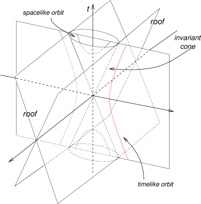
Figure 1: The action of the boost Killing vector on flat spacetime —see [9]—.

In the region below the roof, the boost-rotation symmetric spacetimes can be locally put into the Weyl form, whereas above the roof, the spacetime can be put locally in the form of an Einstein-Rosen wave. The difference between the Weyl and Einstein-Rosen spacetimes and the boost-rotation symmetric spacetimes arises when we consider their global structure. Above the roof, the line element of a boost-rotation symmetric spacetime can be written in the following form:

$$\mbox{d}s^{2}=\frac{1}{c^{2}t^{2}-z^{2}}\{(e^{\nu}z^{2}-e^{\mu}c^{2}t^{2})\mbox{d}z^{2}+c^{2}[2zt(e^{\mu}-e^{\nu})\mbox{d}z\mbox{d}t+(c^{2}e^{\nu}t^{2}-e^{\mu}z^{2})\mbox{d}t^{2}]\}-e^{\nu}\mbox{d}\rho^{2}-\rho^{2}e^{-\mu}\mbox{d}\varphi^{2},$$ (16)

the functions $\mu$ and $\nu$ have the following functional dependence:

$$\mu=\mu(\rho^{2},t^{2}-z^{2}/c^{2}),$$ (17)

$$\nu=\nu(\rho^{2},t^{2}-z^{2}/c^{2}).$$ (18)

In the $(t,\rho,\varphi,z)$ coordinates the region above the roof corresponds to $c^{2}t^{2}>z^{2}$. If (16) corresponds to a vacuum solution of Einstein equations then the function $\mu$ satisfies the wave equation

$$\Box\mu=0,$$ (19)

while $\nu$ can be found by quadratures once $\mu$ has been obtained.

Note now that coordinates $\rho$ and $z$ ($[\rho]=[z]=L$) from line element (16) have dimensions of length, while $t$ has dimensions of time ($[t]=T$). In order to ease our discussion of the Newtonian limit, it will be convenient to make use of dimensionless coordinates. To this end, we assume that our system possesses a characteristic length $\alpha$ and a characteristic time $\tau$. The introduction of a characteristic time in the relativistic regime of the frame theory is superfluous because from a given length one can always construct a time just dividing by the speed of light. However, in the Newtonian limit such canonical choice of speed does not longer exist. This small redundancy is a price one has to pay in order to write the two theories in a common language. Dimensionless coordinates are then given by

$$\widetilde{\rho}=\alpha^{-1}\rho,$$ (20)

$$\widetilde{z}=\alpha^{-1}z,$$ (21)

$$\widetilde{t}=\tau^{-1}t,$$ (22)

$\alpha$ and $\tau$ being constants such that $[\alpha]=L$ and $[\tau]=T$.

In the sequel, it will be convenient to use above the roof coordinates $(\widetilde{b},\widetilde{\rho},\varphi,\tilde{\chi})$, which diagonalize the line element of the spacetime [9]:

$$\mbox{d}s^{2}=\frac{\tau^{2}}{\lambda}e^{\nu}\mbox{d}\widetilde{b}^{2}-\alpha^{2}\left(e^{\nu}\mbox{d}\widetilde{\rho}^{2}-\widetilde{\rho}^{2}e^{-\mu}\mbox{d}\varphi^{2}-{\widetilde{b}^{2}}e^{\mu}\mbox{d}\tilde{\chi}^{2}\right),$$ (23)

where now, $\mu=\mu(\widetilde{\rho}^{2},\widetilde{b}^{2})$, $\nu=\nu(\widetilde{\rho}^{2},\widetilde{b}^{2})$. Note, by the way, that $[\mu]=[\nu]=1$. The coordinate transformation relating the line elements (16) and (23) is given by

$$\widetilde{b}^{2}=\widetilde{t}^{2}-\left(\frac{\alpha^{2}\lambda}{\tau^{2}}\right)\widetilde{z}^{2},$$ (24)

$$\mbox{tanh}^{2}\left(\frac{\alpha\sqrt{\lambda}}{\tau}\,\tilde{\chi}\right)=\left(\frac{\alpha^{2}\lambda}{\tau^{2}}\right)\frac{\widetilde{z}^{2}}{\widetilde{t}^{2}}.$$ (25)

In the rest of this work only dimensionless coordinates will be used, therefore in order to simplify the notation we drop the tilde $\;\widetilde{}\;\,$ from the coordinates $(\widetilde{t},\widetilde{\rho},\varphi,\widetilde{z})$, and $(\widetilde{b},\widetilde{\rho},\varphi,\tilde{\chi})$.

In terms of the $(b,\rho,\varphi,\chi)$ coordinates the field equations take the form,

$$\mu_{,\rho\rho}-\left(\frac{\alpha^{2}\lambda}{\tau^{2}}\right)\mu_{,bb}+\rho^{-1}\mu_{,\rho}-\left(\frac{\alpha^{2}\lambda}{\tau^{2}}\right)b^{-1}\mu_{,b}=0,$$ (26)

$$\left(b^{2}-\left(\frac{\alpha^{2}\lambda}{\tau^{2}}\right)\rho^{2}\right)\nu_{,\rho}=\frac{1}{2}\rho b^{2}\left(\mu_{,\rho}^{2}+\left(\frac{\alpha^{2}\lambda}{\tau^{2}}\right)\mu_{,b}^{2}\right)-\left(\frac{\alpha^{2}\lambda}{\tau^{2}}\right)\rho^{2}b\mu_{,\rho}\mu_{,b}$$

$$\phantom{\left(b^{2}-\left(\frac{\alpha^{2}\lambda}{\tau^{2}}\right)\rho^{2}\right)\nu_{,\rho}=XXXXX}-\left(\left(\frac{\alpha^{2}\lambda}{\tau^{2}}\right)\rho^{2}+b^{2}\right)\mu_{,\rho}+2\left(\frac{\alpha^{2}\lambda}{\tau^{2}}\right)\rho b\mu_{,b},$$ (27)

$$\left(b^{2}-\left(\frac{\alpha^{2}\lambda}{\tau^{2}}\right)\rho^{2}\right)\nu_{,b}=-\frac{1}{2}\rho^{2}b\left(\mu_{,\rho}^{2}+\left(\frac{\alpha^{2}\lambda}{\tau^{2}}\right)\mu_{,b}^{2}\right)+\rho b^{2}\mu_{,\rho}\mu_{,b}$$

$$\phantom{\left(b^{2}-\left(\frac{\alpha^{2}\lambda}{\tau^{2}}\right)\rho^{2}\right)\nu_{,\rho}=XXXXX}-\left(\left(\frac{\alpha^{2}\lambda}{\tau^{2}}\right)\rho^{2}+b^{2}\right)\mu_{,b}+2\rho b\mu_{,\rho}.$$ (28)

Equation (26) corresponds to the wave equation (19), and is the integrability condition for (27) and (28). These field equations suggest considering boost-rotation symmetric solutions of the wave equation (19) as seeds to construct boost-rotation symmetric spacetimes. In fact, one can construct an infinite number of spacetimes of that kind which are regular everywhere but blow up at infinity. These “seeds” lead to spacetimes describing uniformly accelerated particles under the action of an external field. Bičák & Schmidt [9] have shown that the only boost-rotation symmetric solution to (19) which decays to zero at null infinity is $\mu=0$. Therefore, in order to construct (non-trivial) boost-rotation symmetric spacetimes which are as asymptotically flat as possible, one has to consider “seeds” $\mu$ which satisfy the wave equation with sources moving along boost-rotation symmetric orbits, i.e.:

$$\Box\mu=8\pi\sigma,$$ (29)

with $\sigma=\sigma(\rho^{2},b^{2})=\sigma(\rho^{2},t^{2}-\left({\alpha^{2}\lambda}/{\tau^{2}}\right)z^{2})$, $[\sigma]=1$. This strategy will yield spacetimes which will be singular at least along the world lines of the uniformly accelerated particles. Bičák and Schmidt [9]) have briefly discussed tachyonic boost-rotation symmetric sources. Here, only sources moving with speed inferior to that of light ($t^{2}-\left({\alpha^{2}\lambda}/{\tau^{2}}\right)z^{2}<0$) will be considered. Hence, the trajectories of the sources will remain always below the roof. This fact will acquire relevance later, when we try to identify the sources of the gravitational field of the Newtonian limits.

Bičák & Schmidt analysed the fall-off conditions that $\mu$ and $\nu$ have to satisfy for the spacetime to have at least a local null infinity. Moreover, they showed that for metric functions $\mu$ and $\nu$ satisfying the aforementioned asymptotic flatness conditions, it is possible to add suitable constants to both $\mu$ and $\nu$ so that the resulting spacetime has a global null infinity, in the sense that it admits smooth spherical sections. Finally, they also showed that for a $\mu$ satisfying the fall off conditions and vanishing at the origin ($\mu(0,0)=0$), it is possible to construct a spacetime where null infinity is regular except for four points: the “good luck case”. These are the points where the particles enter and leave the spacetime.

As will be shown later —and perhaps not so surprisingly— asymptotic flatness will appear to be a crucial ingredient for the existence of the Newtonian limit of the spacetimes under consideration. Remarkably, non-asymptotically flat solutions (i.e. those describing accelerated particles in uniform fields) can be intuitively constructed from asymptotically flat solutions by sending one of the particles to infinity and at the same time increasing its corresponding mass parameter [5].

The temporal metric and spatial metric of Ehlers’ theory can be constructed from the line element (16) by performing the replacement $c\mapsto{1}/{\sqrt{\lambda}}$ everywhere in (16), where $\lambda$ is the so-called causality constant. Then, the required temporal $t_{ij}$ will be obtained by multiplying the corresponding metric tensor $g_{ij}$ by $\lambda$. In terms of the $(t,z,\rho,\chi$) variables, and up to the two first orders in $\lambda$, these two tensors read

$$t_{ij}=\left(\begin{matrix}{\tau}^{2}\,e^{\nu}-\lambda{\alpha}^{2}\displaystyle{z^{2}}{t^{-2}}\left(e^{\mu}-e^{\nu}\right)&0&0&\lambda\alpha^{2}z\,t^{-1}\left(e^{\mu}-e^{\nu}\right)\cr 0&-\lambda\alpha^{2}e^{\nu}&0&0\cr 0&0&-{{\alpha}^{2}\,\lambda\,{\rho}^{2}}{e^{-\mu}}&0\cr\lambda\alpha^{2}z\,t^{-1}\left(e^{\mu}-e^{\nu}\right)&0&0&-\lambda{\alpha}^{2}e^{\mu}\cr\end{matrix}\right)$$ (30)

$$s^{ij}=\left(\begin{matrix}-{\lambda}\tau^{-2}{e^{-\nu}}&0&0&\lambda\tau^{-2}\,z\,t^{-1}{\left(e^{-\mu}-e^{-\nu}\right)}\cr 0&\alpha^{-2}e^{-\nu}&0&0\cr 0&0&{\alpha}^{-2}\,{{\rho}^{-2}}{e^{\mu}}&0\cr\lambda\tau^{-2}\,z\,t^{-1}{\left(e^{-\mu}-e^{-\nu}\right)}&0&0&\alpha^{-2}e^{-\mu}+{\lambda\,{\tau}^{-2}\,z^{2}}{t^{-2}\left(e^{-\mu}-e^{-\nu}\right)}\cr\end{matrix}\right).$$ (31)

It can be checked that $[t_{ij}]=T^{2}$, and $[s^{ij}]=L^{-2}$.

4 The Newtonian limit of boost-rotation symmetric spacetimes

The natural arena for the discussion of the Newtonian limit of boost-rotation symmetric spacetimes is the region above the roof, i.e. $t^{2}>\left({\alpha^{2}\lambda}/{\tau^{2}}\right)z^{2}$, where the spacetime is radiative. The reason for this is that as one makes $\lambda\to 0$, the region below the roof ($t^{2}<\left({\alpha^{2}\lambda}/{\tau^{2}}\right)z^{2}$) gets squeezed by the roof. That is, the region below the roof disappears in the limit, while the roof becomes the set $\{t=0\}$ —see figure 2—.

Figure 2: The behaviour of the roof as the limit $\lambda\to 0$ is taken.

4.1 Necessary conditions for existence and consequences

The conditions under which the hypothesis of theorem 2.4 are satisfied for the boost-rotation symmetric spacetimes described by either (16) or (23) are summarized in the following proposition.

Proposition 4.1

(Necessary conditions for the existence). Consider the observer field $u^{i}=(\tau^{-1}e^{-\nu/2},0,0,0)$. Necessary conditions for the existence of the Newtonian limit of the family $(M(\lambda),g_{ij}(\lambda))$ of boost-rotation symmetric spacetimes are

• $\nu=\mathcal{O}(\lambda^{0})$, $\mu=\mathcal{O}(\lambda^{0})$, $\mu_{,\rho}=\mathcal{O}(\lambda)$, $\mu_{,b}=\mathcal{O}(\lambda)$

• $\nu_{,\rho}=\mathcal{O}(\lambda)$, $\nu_{,b}=\mathcal{O}(\lambda^{0})$

• $\nu_{,\rho\rho}=\mathcal{O}(\lambda)$, $\nu_{,\rho b}=\mathcal{O}(\lambda)$, $\nu_{,bb}=\mathcal{O}(\lambda^{0})$.

Proof. This follows from using theorem 2.4 and direct inspection. Condition (i) arises from imposing hypothesis (a1) and (a2) of theorem 2.4. In particular, it is important to note that

$$\frac{1}{\lambda}\det s^{ij}=-\frac{1}{\tau^{2}\alpha^{6}}\left(\frac{1}{\rho^{2}}e^{-2\nu}\right).$$ (32)

So, the limit $\lambda\to 0$ may not exist if $\rho=0$. This peculiarity can be easily understood by recalling that the boost-rotation symmetric spaces contain struts or conical singularities on the axis $\rho=0$. These singularities represent the particles undergoing uniform acceleration.

Along the same lines, condition (ii) of lemma 4.1 arises from imposing hypothesis (b1) and (b2) of theorem 2.4. In particular, the condition $\nu_{,\rho}=\mathcal{O}(\lambda)$ and $\nu_{,b}=\mathcal{O}(\lambda^{0})$ appears from assuming that the limit

$$\lim_{\lambda\to 0}F=\lim_{\lambda\to 0}\frac{1}{\lambda}\mbox{d}u^{\bullet}$$ (33)

exists. This is because

$$u^{\bullet}=t_{ij}u^{i}\mbox{d}x^{j}=\tau e^{\nu/2}\mbox{d}b=\tau e^{\nu/2}\mbox{d}t+\mathcal{O}(\lambda),$$ (34)

where we have used the relation $b=t+\mathcal{O}(\lambda)$. So, at the end of the day one has

$$F=-\frac{\tau}{2\lambda}e^{\nu/2}\left(\nu_{,\rho}\mbox{d}t\wedge\mbox{d}\rho+\nu_{,z}\mbox{d}t\wedge\mbox{d}z+\mathcal{O}(\lambda)\right),$$ (35)

and hence the need of $\nu_{,\rho}=\mathcal{O}(\lambda)$ and $\nu_{,b}=\mathcal{O}(\lambda^{0})$ for the limit to exist. In the remainder, we will show that this condition has something to do with asymptotic flatness. Most boost-rotation symmetric spacetimes which are not at least locally asymptotically flat will not satisfy it.

Finally, condition (ii) stems from requiring the existence of the limit as $\lambda\to 0$ of the Riemann tensor. $\Box$

Using the field equations (26)-(28) it is not hard to draw some immediate consequences of proposition 4.1.

Proposition 4.2

(Consequences of the necessary conditions). Assume that the hypothesis of proposition 4.1 hold. Then,

• $$\mu_{,\rho}=\mathcal{O}(\lambda),\qquad\mu_{,\rho\rho}=\mathcal{O}(\lambda);$$ (36)

• $$\mu=\overset{\circ}{\mu}(b^{2})+\lambda\Xi(\rho^{2},b^{2}),$$ (37)

  $$\nu=\overset{\circ}{\nu}(b^{2})+\lambda\Phi(\rho^{2},b^{2}),$$ (38)

  where $\Xi=\mathcal{O}(\lambda^{0})$, $\Phi=\mathcal{O}(\lambda^{0})$, and according to the field equations $\overset{\circ}{\nu}_{,b}=-\overset{\circ}{\mu}_{,b}$;

• $$\sigma=\lambda\Sigma(\rho^{2},b^{2}),$$ (39)

  where $\Sigma=\mathcal{O}(\lambda^{0})$.

Proof. The $\lambda$-dependencies given in (i) come directly from taking the limit $\lambda\to 0$ in the field equation (27) and using the result in (26). Consequence (ii) follows from the last discussion and from (ii) in proposition 4.1. Finally, (iii) comes from using (i) and (ii) in the wave equation with sources,

$$\mu_{,\rho\rho}+\rho^{-1}\mu_{,\rho}-\left(\frac{\alpha^{2}\lambda}{\tau^{2}}\right)\mu_{,bb}-\left(\frac{\alpha^{2}\lambda}{\tau^{2}}\right)b^{-1}\mu_{,b}=8\pi\sigma.$$ (40)

$\Box$

4.2 The role of asymptotic flatness

So far, asymptotic flatness of the boost-rotation symmetric spacetimes (or the lack of it) has not entered our analysis. Ehlers argued that the notion of asymptotic flatness should play a crucial role in the existence of Newtonian limits [14]. This observation suggests the possibility that spacetimes describing accelerated particles in uniform (gravitational) fields may not possess a Newtonian limit proper.

Following reference [9], we will consider that a given metric function $\mu$ —satisfying a non-homogeneous wave equation— is said to be compatible with asymptotic flatness if $\Omega^{-1}\mu$ is smooth on null infinity, where $\Omega$ is a suitable conformal factor defining null infinity. This means that it should have (at least) the following asymptotic behaviour:

$$\mu=\mu_{1}\Omega+\mathcal{O}(\Omega^{2}).$$ (41)

Consider for example the conformal factor,

$$\Omega=\frac{1}{\left({\tau^{2}}/{\alpha^{2}\lambda}\right)t^{2}-\rho^{2}-z^{2}}\,,$$ (42)

which is valid for the region $\left({\tau^{2}}/{\alpha^{2}\lambda}\right)t^{2}>\rho^{2}-z^{2}$. Now, consider a metric function $\mu^{*}$ not compatible with asymptotic flatness. For example,

$$\mu^{*}=\mu_{-1}\Omega^{-1}+\mu_{0}+\mu_{1}\Omega+\mathcal{O}(\Omega^{2}),$$ (43)

$$\phantom{\mu^{*}}=\mu_{-1}\left(\left(\frac{\tau^{2}}{\alpha^{2}\lambda}\right)t^{2}-\rho^{2}-z^{2}\right)+\mathcal{O}(\Omega^{0}),$$ (44)

where $\mu_{-1}=\mathcal{O}(\lambda^{0})$. Whence,

$$\mu^{*}_{,\rho}=-2\rho\mu_{-1}+\cdots,$$ (45)

so that $\overset{\circ}{\mu}\,^{*}\!_{,\rho}\neq 0$, and accordingly $\overset{\circ}{\nu}_{,\rho}\,^{*}\neq 0$. That is, condition (ii) of proposition 4.1 is not satisfied, and thus the boost-rotation symmetric spacetime to be obtained from the seed function $\mu^{*}$ does not have a properly defined Newtonian limit. This last result shows that, in fact, asymptotic flatness is a prerequisite for the existence of a Newtonian limit. This should not be a surprise because Newton’s theory, as pointed out by Ehlers, is actually a theory of isolated bodies. Several ways to impose it have been suggested in the literature —see in particular [20]—. Note, however, that a decay of the form

$$\mu=\mu_{0}+\mu_{1}\Omega+\mathcal{O}(\Omega^{2}),$$ (46)

is still compatible with condition (ii) of proposition 4.1. This particular class of boost-rotation symmetric spacetimes could still have a Newtonian limit.

As should be expected, the asymptotic flatness of the general relativistic solution leaves an imprint on the asymptotic behaviour of its Newtonian limit. We have the following result.

Proposition 4.3

(Consequences of asymptotic flatness). Let $\mu$ be a solution of the wave equation with sources (29) compatible with asymptotic flatness. Then it follows that

• $$\overset{\circ}{\nu}_{,b}=\overset{\circ}{\mu}_{,b}=0;$$ (47)

• similarly, for fixed $t$ and $z$ one has,

  $$\Xi\sim\frac{C}{\rho^{2}},\qquad\Phi\sim-\frac{C}{\rho^{2}},$$ (48)

  for large $\rho$, where $C$ is a constant.

Proof. Consider the conformal factor given in (42). It is not hard to see that

$$\Omega=\frac{1}{t^{2}}\left(\frac{\alpha^{2}\lambda}{\tau^{2}}\right)+\frac{\rho^{2}+z^{2}}{t^{4}}\left(\frac{\alpha^{2}\lambda}{\tau^{2}}\right)^{2}+O(\lambda^{3}).$$ (49)

As mentioned before, a function $\mu$ compatible with asymptotic flatness will be of the form

$$\mu=\mu_{1}\Omega=\mathcal{O}(\Omega^{2}),$$ (50)

where $\mu_{1}=\mathcal{O}(\lambda^{0})$, and $\partial_{\Omega}\mu_{1}=0$. Hence one has

$$\mu=\frac{\mu_{1}}{t^{2}}\left(\frac{\alpha^{2}\lambda}{\tau^{2}}\right)+O(\lambda^{2}).$$ (51)

Accordingly $\overset{\circ}{\mu}_{,b}=0$ —cfr. (ii) in proposition 4.2—. Thus, from (ii) in (4.2) one has $\overset{\circ}{\nu}_{,b}=\overset{\circ}{\nu}_{,t}=0$. In order to prove (iii), let us consider the conformal factor

$$\Omega^{\prime}=\frac{1}{\rho^{2}+z^{2}-\left({\tau^{2}}/{\alpha^{2}\lambda}\right)t^{2}},$$ (52)

in the domain in which it is positive. Then, asymptotically one has $\Omega^{\prime}\sim 1/\rho^{2}$, from which (ii) follows. $\Box$

4.3 Interpretation and sources

We are now in the position of discussing the Newtonian (gravitational) potential of those boost-rotation symmetric spacetimes possessing a Newtonian limit and describing the sources that give rise to them. Because of proposition (4.2) one has that the connection form —see equation (35)— is given by

$$F=-\frac{1}{2}{\Phi_{,\rho}}(e^{\nu/2})\mbox{d}t\wedge\mbox{d}\rho-\frac{1}{2}{\Phi_{,z}}(e^{\nu/2})\mbox{d}t\wedge\mbox{d}z+\mathcal{O}(\lambda),$$ (53)

and because of (i) in lemma 4.1 then $e^{\nu/2}=\mathcal{O}(\lambda^{0})$ and therefore

$$\overset{\circ}{F}=-\frac{1}{2}\Phi_{,\rho}\mbox{d}b\wedge\mbox{d}\rho-\frac{1}{2}\Phi_{,z}\mbox{d}b\wedge\mbox{d}z$$ (54)

The last result, along with theorem 2.2 and corollary 2.3, indicates that $-\Phi/2$ is the Newtonian potential as measured by the rigid observers $u^{i}$. In reference [9] it was argued that because of equation (29) and since “$\Box\to\Delta$” in the $\lambda\to 0$ limit, it is suggestive to interpret $\mu/2$ as a (Newtonian) gravitational potential. It was also noticed that in the weak field approximation (i.e. weak sources) and for $t\approx 0$ one has

$$g_{00}=e^{\mu}\approx 1+\mu,$$ (55)

which brings further support to their point of view. Here we want to make the point that this is only true if one enforces the requirement of asymptotic flatness. To see this, divide field equation (27) by $\tau^{-2}\lambda$ and take the limit as $\lambda\to 0$. Recalling that $b\to t$ as $\lambda\to 0$ one obtains

$$\tau^{2}t^{2}\Phi_{,\rho}=\frac{1}{2}\alpha^{2}\rho t^{2}(\overset{\circ}{\mu}_{,t})^{2}-\tau^{2}t^{2}\Xi_{,\rho}+2\alpha^{2}\rho t\overset{\circ}{\mu}_{,t}.$$ (56)

Thus, only if the boost-rotation symmetric spacetime is asymptotically flat one will have that $\overset{\circ}{\mu}_{,t}=0$ and accordingly $\Xi_{,\rho}=-\Phi_{,\rho}$. In addition to this, $\Xi_{,z}=-\Phi_{,z}$ follows from an analogous discussion involving equation (28). For the Newtonian limit of the non-asymptotically flat spacetimes described in §4.2, whose metric seed function $\mu$ is of the form $\mu=\mu_{0}+\mathcal{O}(\Omega)$, the interpretation of $\mu/2$ as a potential is not valid. This example illustrates the subtle —but crucial— differences between the notions of weak field approximation and Newtonian limit. The weak limit approximation is still a curved spacetime theory valid for sources which in some sense are moving slowly. Recall that the boost-rotation symmetric spacetimes are time symmetric, so that the uniformly accelerated particles start moving from rest at $t=0$. Thus, in our case, this weak field approximation should only be correct for $t\approx 0$, where they will still be moving slowly. On the other hand, in the Newtonian theory there is no restriction to the speed an object can attain, as long as it remains bounded for finite times. Accordingly, it is valid for all times. Finally observe that if one constructs a function $\mu$ such that $\overset{\circ}{\mu}_{,b}=0$ then one would indeed have $\Xi_{,\rho}=-\Phi_{,\rho}$ and $\Xi_{,z}=-\Phi_{,z}$.

Given a boost-rotation symmetric source $\sigma=\sigma(\rho^{2},t^{2}-\lambda{\alpha^{2}}z^{2}/{\tau^{2}})$, then by means of Kirchoff integrals its is possible to construct retarded $(\mu_{+})$ and advanced $(\mu_{-})$ fields of the form

$$\mu_{\pm}=\frac{1}{8\pi}\int_{\mbox{{\SYM R}}^{4}}\frac{\sigma\left(\rho^{\prime 2},t^{\prime 2}-({\alpha^{2}\lambda}/{\tau^{2}})z^{\prime 2}\right)}{\sqrt{(\rho-\rho^{\prime})^{2}+(z-z^{\prime})^{2}}}\,\delta\left(\frac{\alpha}{\tau}\sqrt{\lambda}\sqrt{(\rho-\rho^{\prime})^{2}+(z-z^{\prime})^{2}}\mp(t-t^{\prime})\right)\mbox{d}^{4}x^{\prime},$$ (57)

where the integral is evaluated over the whole Minkowski spacetime. We note that the boost-rotation symmetric source can be very complicated and posses all sorts of multipole structures —represented by derivatives of the $\delta$-function—. The relevance of these advanced and retarded solutions for our purposes is that by considering linear combinations of the functions $\mu_{\pm}$, one can construct [9] a metric function $\mu$ that is an analytic function of $\rho^{2}$ and $t^{2}-\lambda z^{2}$ outside the sources, and which is asymptotically regular at the fixed points of the boost-symmetry on null infinity, namely

$$\mu=a\mu_{+}+(1-a)\mu_{-},$$ (58)

where $a$ is suitable constant. Recalling that $\sigma=\lambda\Sigma$, where $\Sigma=\mathcal{O}(\lambda^{0})$ is analytic in $\lambda$ so that $\lim_{\to 0}\Sigma(\rho^{2},t^{2}-\lambda\alpha^{2}z^{2}/\tau^{2})$ does not depend on $z$, one has that

$$\lim_{\lambda\to 0}\frac{\mu}{\lambda}=\frac{a}{8\pi}\int_{\mbox{{\SYM R}}^{4}}\frac{\overset{\circ}{\Sigma}\;\delta(t-t^{\prime})}{\sqrt{(\rho-\rho^{\prime})^{2}+(z-z^{\prime})^{2}}}\,\mbox{d}^{4}x^{\prime}$$

$$\phantom{\lim_{\lambda\to 0}\frac{\mu}{\lambda}XXXXXXXXXX}+\frac{(1-a)}{8\pi}\int_{\mbox{{\SYM R}}^{4}}\frac{\overset{\circ}{\Sigma}\;\delta(t-t^{\prime})}{\sqrt{(\rho-\rho^{\prime})^{2}+(z-z^{\prime})^{2}}}\,\mbox{d}^{4}x^{\prime},$$ (59)

$$\phantom{\lim_{\lambda\to 0}\frac{\mu}{\lambda}}=\frac{1}{8\pi}\int_{\mbox{{\SYM R}}^{3}}\frac{\overset{\circ}{\Sigma}|_{t}}{\sqrt{(\rho-\rho^{\prime})^{2}+(z-z^{\prime})^{2}}}\,\mbox{d}^{3}x^{\prime}.$$ (60)

Thus, for an boost-rotation symmetric spacetime arising from an asymptotically flat seed $\mu$ one gets that —cfr. equation (56)—,

$$\Phi=-\frac{1}{8\pi}\int_{\mbox{{\SYM R}}^{3}}\frac{\Sigma(\rho^{\prime 2},t^{2})}{\sqrt{(\rho-\rho^{\prime})^{2}+(z-z^{\prime})^{2}}}\mbox{d}^{3}x^{\prime}.$$ (61)

Consequently, the potential $\Phi$ satisfies the Poisson equation with moving sources:

$$\Delta(-\Phi/2)=4\pi\Sigma(\rho^{2},t^{2}).$$ (62)

Note, in particular, the minus sign in the source term. In the Newtonian limit, the boost-rotation symmetric source has been replaced by a moving cylindrically symmetric source analytic in $\rho^{2}$ and $t^{2}$. We finish this discussion by recalling that the boost-rotation symmetric source $\sigma$ is such that the amount of negative masses balances exactly the amount of positive masses. That is,

$$\int_{\mbox{{\SYM R}}^{3}}\sigma\left(\rho^{2},t^{2}-\left({\alpha^{2}\lambda}/{\tau^{2}}\right)z^{2}\right)\mbox{d}^{3}x^{\prime}=0.$$ (63)

It then follows that $\Sigma(\rho^{2},t^{2})$ will inherit this property. Indeed,

$$\int_{\mbox{{\SYM R}}^{3}}\Sigma(\rho^{2},t^{2})\mbox{d}^{3}x^{\prime}=0.$$ (64)

5 Examples

We now proceed to briefly discuss the Newtonian limits of some examples of boost-rotation symmetric spacetimes. As noted in the introductory sections, the first problem one has to face in order to proceed with this discussion is how to transcribe the exact general relativistic solutions —which almost always are expressed in terms of “natural” units for which $c=1$— into the language of the theory of frames. There is no canonical/unique way to do this. Indeed, one could for example, introduce the causality constant $\lambda$ in such a way into the Schwarzschild solution so that instead of the expected Newtonian limit of the potential due to a point mass one obtains a vanishing potential. Thus, the criteria for choosing a particular transcription rule is that it provides an interesting Newtonian limit. In our particular case, consistent with the discussion of section 3, we put forward the transition rules

$$\rho_{BHS}\mapsto\alpha\rho,$$ (65)

$$z_{BHS}\mapsto\alpha z,$$ (66)

$$t_{BHS}\mapsto\frac{\tau}{\alpha\sqrt{\lambda}}t,$$ (67)

where $\rho_{BHS}$, $z_{BHS}$, $t_{BHS}$ are the $\rho$, $z$, $\tau$ coordinates used by Bičák, Hoenselaers and Schmidt [5, 6] (Bonnor [11] labels them $\eta$, $\zeta$, $\tau$), and $\rho$, $z$ and $t$ are the dimensionless coordinates used throughout most of this article. In order to write the expressions in a more compact fashion, we define the dimensionless quantity

$$\zeta=\left(\rho^{2}+z^{2}-\frac{\tau^{2}}{\alpha^{2}\lambda}t^{2}\right).$$ (68)

5.1 The two monopoles solution

In [9], Bičák & Schmidt have constructed what is arguably the simplest non-trivial example of a boost-rotation symmetric “potential” $\mu$: that obtained from the superposition of retarded and advanced potentials due to two uniformly accelerated point particles, one with a positive mass, and the other with a negative one. The function $\mu$ thus obtained is by construction compatible with asymptotic flatness. Therefore, the boost-rotation symmetric spacetime arising from it will also be asymptotically flat modulo the usual problems at the intersection of the light cone through the origin with null infinity. Because of its asymptotic flatness, the Newtonian limit is expected to exist, and therefore it can be determined by simply looking at $\mu$ (cfr. §4.2). In terms of the dimensionless coordinates $(t,\rho,\chi,z)$ one has that

$$\mu=-\frac{4mG\lambda}{\alpha\sqrt{(\zeta-1)^{2}+4\rho^{2}}},$$ (69)

where the constant $m$ has dimensions of mass and $\zeta$ given by (68). As explained previously, a non-trivial Newtonian limit for boost-rotation spacetimes will only exist, strictly speaking, for $t=0$ —the sources of the wave equation (29) and of the associated limiting Poisson equation vanish “above the roof”—. Thus, the direct naive evaluation of the limit $\lim_{\lambda\to 0}{\mu}/{\lambda}$ yields zero. In order to extract a non-trivial limit out of (69) we expand around $t=0$, so that

$$\mu=-\frac{4mG\lambda}{\alpha\sqrt{4\rho^{2}+(\rho^{2}+z^{2}-1)^{2}}}+\mathcal{O}(t^{2}).$$ (70)

Thus, one could say that the Newtonian potential corresponding to the relativistic two-monopole boost-rotation symmetric spacetime is, for $t\approx 0$ given by

$$\Phi\approx\frac{2mG}{\alpha\sqrt{4\rho^{2}+(\rho^{2}+z^{2}-1)^{2}}}.$$ (71)

Figure 3: Level curves of the Newtonian potential due to the two monopole solution for $t\approx 0$.

The latter inherits the axial symmetry from the relativistic solution. Furthermore, it is singular at two points lying on the $z$-axis, $(\rho_{sing},\varphi_{sing},z_{sing})=(0,0,1)$ —see figure 3—. These singularities are naturally identified with the presence of two point-particles. Note that the potential is —by construction— time independent. Thus, the Newtonian limit for early times is a strictly static Newtonian potential in which the sources are not moving. Another remarkable feature of the solution is that, as can readily be checked, the masses of the two point particles giving rise to the Newtonian field have the same (positive) sign.

5.2 The Curzon-Chazy $(01)$-pole particles solution.

This example of boost-rotation symmetric spacetimes was first given in [6]. It was constructed from the classical Bonnor-Swaminarayan solution [12] by considering an appropriate limiting procedure. This solution is interpreted as the superposition of a monopole particle and a dipole particle. Again, by construction, the “seed” function is compatible with asymptotic flatness so that a Newtonian limit is bound to exist. In this case one has

$$\mu=-\frac{{D}G\lambda}{\alpha^{2}}\frac{\zeta(\zeta-1)+2\rho^{2}}{\left((\zeta-1)^{2}+4\rho^{2}\right)^{3/2}},$$ (72)

where ${D}$ a constant of dipolar nature ($[{D}]=ML$), and $\zeta$ as in (68). Again, expanding $\mu$ around $t=0$ one finds that

$$\Phi=\frac{{D}G}{\alpha^{2}}\left(\frac{(\rho^{2}+z^{2})(\rho^{2}+z^{2}-1)+2\rho^{2}}{(4\rho^{2}+(\rho^{2}z^{2}-1)^{2})^{(3/2)}}\right).$$ (73)

The Newtonian potential is again singular at $(\rho_{sing},\varphi_{sing},z_{sing})=(0,0,\pm\sqrt{t^{2}+1})$. Looking at the level curves of the potential (73) one can perceive the fingerprints of the “dipole structure” of the point particles.

5.3 The Generalized Bonnor-Swaminarayan solution

This solution was obtained in [5] by using Ernst’s regularization procedure [15]. It describes two identical particles symmetrically located with respect to the plane $z=0$ and uniformly accelerated along the axis $\rho=0$. The interest of this example for our purposes lies in the known fact that this spacetimes is not asymptotically flat. In this case one has

$$\mu=\frac{{D}G\lambda}{\alpha^{2}}\left(1-\frac{1}{\sqrt{(\zeta-1)^{2}+4\rho^{2}}}\right)+\left(2\rho^{2}-\zeta\right),$$ (74)

where again $[{D}]=ML$, and $\zeta$ given by (68). It can be readily seen that $\mu_{,\rho}=\mathcal{O}(\lambda^{0})$, and thus, by propositions 4.1 and 4.2, it does not possess a proper Newtonian limit.

Figure 4: Level curves of the Newtonian potential due to the Curzon-Chazy $(01)$-pole solution.

5.4 The C metric.

We conclude our discussion of examples by considering the epitome of the boost-rotation symmetric spacetimes: the C metric. Bonnor [11] was the first to cast it in the form which exhibits its boost-rotation symmetric nature. The metric function $\mu$ arises from solutions to the wave equation with sources which are uniformly accelerated rods moving along the $z$ direction. In terms of our dimensionless coordinates one has

$$\mu=\ln\left(\frac{1}{4\omega^{2}}\frac{\sqrt{(\zeta-\beta)^{2}+4\beta\rho^{2}}+(\zeta-2\rho^{2})-\beta}{\sqrt{(\zeta-1)^{2}+4\rho^{2}}+(\zeta-2\rho^{2})-1}\right).$$ (75)

The classical parameters $m$ and $A$ are related to the parameters $\alpha$, $\beta$ and $\omega$ via,

$$\alpha^{2}=2(z_{2}-z_{1}),\qquad\alpha^{2}\beta=2(z_{2}-z_{3}),$$ (76)

where $z_{1}$, $z_{2}$, $z_{3}$ are solutions of

$$2A^{4}z^{3}-A^{2}z^{2}+m^{2}=0.$$ (77)

It is assumed that the parameters $m$ and $A$ are such that the latter has 3 real solutions, and that $z_{2}$ is the biggest root. Finally,

$$\omega^{2}=4m^{2}A^{-6}\alpha^{-8}(\beta-1)^{-2}.$$ (78)

The points where $\mu$ is singular can be identified with sources. A simple calculation shows then that this happens at $(0,0,z_{sing})$ with $z_{sing}\in(-\sqrt{\beta},-1)\cup(1,\sqrt{\beta})$ if $\beta>1$ or $z_{sing}\in(-1,-\sqrt{\beta})\cup(\sqrt{\beta},1)$ if $\beta<1$. If $\beta=1$, then no singular points occur, and the C metric is in fact Minkowski spacetime, that is, there are no sources. This seems to indicate that the geometry is induced by the presence two rods of finite length symmetrically located along the $z$-axis. This agrees with the description given by Bičák and Schmidt [9] on how to construct the C-metric from a “seed”.

Now, a direct evaluation shows that the conditions $\mu_{,\rho}=\mathcal{O}(\lambda)$ and $\mu_{,z}=\mathcal{O}(\lambda)$ needed for the existence of a Newtonian limit of the C-metric do not hold unless

$$\beta=1+\beta_{1}\lambda+\mathcal{O}(\lambda).$$ (79)

Assuming the latter one finds

$$\Phi=\frac{\beta_{1}}{2\sqrt{4\rho^{2}+(\rho^{2}+z^{2}-1)^{2}}},$$ (80)

at $t\approx 0$. That is, one recovers the potential of the two monopoles solution. This is in agreement with the results by Bonnor, who concluded that in the weak field limit the C metric describes two accelerated monopoles [11].

6 Conclusions

We have discussed the Newtonian limit of boost-rotation symmetric spacetimes. It has been shown that the existence, or not, of a Newtonian limit depends on the asymptotic flatness of the relativistic spacetime. As discussed in the main text, boost-rotation symmetric spacetimes posses two Killing vectors: an axial one which is inherited by the Newtonian limit, and a boost Killing vector. The boost Killing vector field is not inherited in any clear way by the Newtonian limit as this symmetry is of relativistic nature.

In order to construct “seed” fields $\mu$ which are analytical, one has to resort to suitable combinations of advanced and retarded fields due to boost-rotation symmetric sources for which the total amount of mass is zero. That is, one has to allow for the presence of negative masses. The presence of regions of space containing negative mass is preserved in the Newtonian limit in such a way that the total amounts of positive and negative masses cancel exactly each other.

The standard interpretation of the boost-rotation symmetric spacetimes regards them as models of uniformly accelerated particles. As has been shown with the examples, the Newtonian limits are well defined for all times, however the interpretation of particles moving in an uniformly accelerated fashion is only valid for early times $t\approx 0$. The time dependence of Newtonian potential can be traced back to the fact that the sources in the relativistic regime carry their own source of motion: the struts or conical singularities joining them. In other words, the motion of the Newtonian sources is the Newtonian consequence of the singularities in the relativistic boost-rotation symmetric spacetimes. Summarizing, the Newtonian limits obtained exhibit several unphysical features; however, all of them can be traced back to problems already existing in the general relativistic solutions. Whether the struts and strings appearing in the general relativistic solutions here considered are “terribly” unphysical or not, is nevertheless a matter of taste.

Finally, in §4.3 it has been shown that the potential suggested by a weak field analysis coincides, in the case where asymptotic flatness is required, with the Newtonian potential obtained through our analysis. There has been some discussion in the literature —cfr. [9, 11]— in what regards writing the potentials as a combination of advanced and retarded fields. This discussion lies beyond the realm of our analysis, because in a purely Newtonian theory information travels with infinite speed. In order to look at these effects one would have to look at the post-Newtonian expansions of the solutions.

Appendix: the axioms of Ehlers’ theory

The axioms of Ehlers’ frame theory and their consequences are discussed extensively for example in [17]. However, this reference is not so readily available. Therefore, for the sake of completeness we present them here. The axioms shown here are an adapted version of those appearing in Lottermoser’s thesis. The first set of axioms deals with the objects that the frame theory will attempt to describe.

Axiom 6.1

(On the objects described by the frame theory). The mathematical objects of the theory are collections $(M,t_{ij},s^{ij},\Gamma^{i}_{jk},T^{ij},\lambda,G)$ for which the following holds:

• $M$ is a 4-dimensional Hausdorff manifold endowed with a connection,

• $t_{ij}$, $s^{ij}$ and $T^{ij}$ are symmetric tensor fields on $M$ (temporal metric, spatial metric, matter tensor),

• $\Gamma^{i}_{jk}$ is a torsion-free linear connection on $M$ (gravitational field),

• $\lambda$ and $G$ are real numbers (causality and gravitational constant).

The axioms require some minimal differentiability conditions. Thus, $t_{ij}$, $s^{ij}$, $T^{ij}$ and $\Gamma^{i}_{jk}$ should at least be $C^{1}$ and $M$ at least a $C^{3}$ manifold.

The next set of axioms describes, by means of observable quantities, how the objects of the frame theory ought to be interpreted.

Axiom 6.2

(Physical interpretation)

• Observers move along timelike curves, that is, curves such that their tangent vector $u^{i}$ satisfies $t_{ij}u^{i}u^{j}>0$ everywhere. The space directions of an observer are the tangent vectors $v^{i}\neq 0$ along the curves which are orthogonal to $u^{i}$ with respect to $t_{ij}$: $t_{ij}u^{i}v^{j}=0$.

• Time intervals are defined along timelike curves. Let $s$ be the curve parameter. Then for the infinitesimal time interval the following holds:

  $$dt=\sqrt{t_{ij}u^{i}u^{j}}ds.$$ (81)

• Space intervals are defined along spacelike curves, i.e. curves such that for their tangent vector $v^{i}$ there exists a 1-form $\omega_{i}$ which satisfies

  $$v^{i}=\omega^{i}_{\bullet},$$ (82)

  and $s^{ij}\omega_{i}\omega_{j}>0$. If $s$ is again the curve parameter, then the spatial interval is given by

  $$dl=\sqrt{s^{ij}\omega_{i}\omega_{j}}ds.$$ (83)

The following 2 axioms establish the conditions a mathematical model should satisfy in order to be called a “solution of the frame theory”.

Axiom 6.3

(Metric axioms)

• At each point of the spacetime, there exists at least one timelike vector,

  $$\forall p\in M\;\;\exists u^{i}\in T_{p}M:\;\;t_{ij}u^{i}u^{j}>0.$$ (84)

• At each point of the spacetime, the temporal metric is positive definite at each observer orthogonal subspace of the cotangent space. That is,

  $$\forall p\in M,\;\;u^{i}\in T_{p}M,\;\;t_{ij}u^{i}u^{j}>0$$ (85)

  $s^{ij}$ is positive definite in the set $H^{+}(u^{i})=\{\omega\in T_{p}^{*}M|\;\;\omega_{i}v^{j}=0\}$.

• the temporal and spatial metrics are related to each other via,

  $$t_{ij}s^{jk}=-\lambda\delta_{i}^{k}.$$ (86)

Axiom 6.4

(Connection axioms)

• The connection $\Gamma^{i}_{jk}$ is compatible with the temporal and spatial metrics metrics, i.e.

  $$t_{ij;k}=0,\qquad s^{ij}_{\phantom{ij};k}=0$$ (87)

• the curvature tensor $R^{i}_{jkl}=2(\Gamma^{i}_{j[l,k]}+\Gamma^{i}_{m[k}\Gamma^{m}_{l]j})$ of $\Gamma^{i}_{jk}$ possesses the property,

  $$R^{i\phantom{j}k}_{\phantom{i}j\bullet l}=R^{k\phantom{l}i}_{\phantom{k}l\bullet j}.$$ (88)

References

- [1] J. Bičák, Gravitational radiation from uniformly accelerated particles in general relativity, Proc. Roy. Soc. Lond. A 302, 201 (1968).
- [2] J. Bičák, On exact radiative sources representing finite sources, in Galaxies, axisymmetric systems and relativity, edited by M. A. H. MacCallum, Cambridge University Press, 1985.
- [3] J. Bičák, Radiative properties of space-times with the axial and boost symmetries, in Gravitation and geometry, edited by W. Rindler & A. Trautman, Bibliopolis, 1987.
- [4] J. Bičák, Selected solutions of Einstein’s field equations: their role in general relativity and astrophysics, in Einstein Field Equations and Their Physical Implications (Selected essays in honour of Juergen Ehlers), edited by B. G. Schmidt, Springer Verlag, 2000.
- [5] J. Bičák, C. Hoenselaers, & B. G. Schmidt, The solutions of the Einstein equations for uniformly accelerated particles without nodal singularities. I. Freely falling particles in external fields, Proc. Roy. Soc. Lond. A 390, 397 (1983).
- [6] J. Bičák, C. Hoenselaers, & B. G. Schmidt, The solutions of the Einstein equations for uniformly accelerated particles without nodal singularities. II. Self-accelerating particles, Proc. Roy. Soc. Lond. A 390, 411 (1983).
- [7] J. Bičák & A. Pravdová, Symmetries of asymptotically flat electrovacuum space-times and radiation, J. Math. Phys. 39, 6011 (1998).
- [8] J. Bičák & B. G. Schmidt, Isometries compatible with gravitational radiation, J. Math. Phys. 25, 600 (1984).
- [9] J. Bičák & B. G. Schmidt, Asymptotically flat radiative space-times with boost-rotation symmetry: the general structure, Phys. Rev. D 40, 1827 (1989).
- [10] H. Bondi, Negative mass in general relativity, Rev. Mod. Phys. 29, 423 (1957).
- [11] W. B. Bonnor, The sources of the vacuum C-metric, Gen. Rel. Grav. 15, 535 (1983).
- [12] W. B. Bonnor & N. Swaminarayan, An exact solution for uniformly accelerated particles in general relativity, Z. Phys. 177, 240 (1964).
- [13] G. Dautcourt, Post-Newtonian limit of the Newton-Cartan theory, Class. Quantum Grav. 14, A109 (1997).
- [14] J. Ehlers, The Newtonian limit of General Relativity, in Understanding physics, edited by A. K. Richter, Copernicus Gesellschaft, 1998.
- [15] F. J. Ernst, Generalized C metric, J. Math. Phys. 19, 1986 (1978).
- [16] S. Hawking & S. F. Ross, Pair production of black holes on cosmic strings, Phys. Rev. Lett. 75, 3382 (1995).
- [17] M. Lottermoser, Über den Newtonschen Grenzwert der Allgemein Relativitätstheorie ind die relativistische Erweiterung Newtoscher Anfangsdaten, PhD thesis, Lüdwig-Maximilians Universität München, 1988.
- [18] R. Penrose, Asymptotic properties of fields and space-times, Phys. Rev. Lett. 10, 66 (1963).
- [19] V. Pravda & A. Pravdová, Boost-rotation symmetric spacetimes —review, Czech. J. Phys. 50, 333 (2000).
- [20] A. Trautman, Comparison of Newtonian and Relativistic theories of space-time, in Perspectives in Geometry and Relativity, edited by B. Hoffmann, page 425, Indiana University Press, 1966.
- [21] J. A. Valiente Kroon, On Killing vector fields and Newman-Penrose constants, J. Math. Phys. 41, 898 (2000).
- [22] J. Winicour, Newtonian gravity on the null cone, J. Math. Phys. 25, 1193 (1983).