Spinning particles in gravitational wave spacetime

Abstract

The dynamics of pseudo-classical spinning particles in spacetime of gravitational plane waves of general polarization and harmonic profile is studied. The resulting equations of motion are solved exactly and the results are compared with those of the other approaches. The relative accelerations of nearby particles is also calculated.

PACS numbers: 04.20.-q, 04.25.-g, 04.30.-Nk
Keywords: spinning particles, gravitational waves

1 Introduction

The dynamics of particles in curved spacetime has been an important part of the theories of gravitation. The dynamics of test particles, i.e., particles without any internal structure was studied in the early stages of the development of general relativity. Recently, there has been a growing interest in the problem of motion of spinning particles (some references may be found in [1]).

Rietdijk and van Holten [2] has obtained a general set of equations of the symmetries of the spinning particles in an arbitrary curved spacetime. Similar equations has been obtained in [3] from a more general action. These equations constitutes a Grassmann valued extension of the Killing equations for the symmetries of the spacetime manifold. These ideas was further investigated in [4] and was applied to the case of Schwarzschild spacetime in [5] and to Reissner-Nordstrom spacetime in [6]. The canonical structure of the theory and the equivalent Dirac formulation of the quantum theory has been derived in [7]. Equations for the world-line deviations of spinning particles was obtained in [8].

The aim of the present paper is to study the motion of spinning particles in the spacetime of an exact plane gravitational wave following the ideas presented in the references mentioned above. This problem has been studied previously in the framework of Papapetrou-Dixon description of spinning particles in [1] and [9, 10, 11]. In [1] a linearized version of Papapetrou-Dixon equations was applied to the case of a weak plane gravitational wave of arbitrary polarization and harmonic profile. In [10] a linearly polarized wave of arbitrary profile (and in particular, a square gravitational wave pulse) was considered and a set of exact solutions was presented in some rather special circumstances. The general solution of those equations could only be found numerically, of course.

There is a simpler version of Papapetrou-Dixon equations. This is basically obtained by replacing the usual supplementary condition $p\cdot s=0$ by the so called Pirani supplementary condition $v\cdot s=0$. A similar calculation has been performed along the lines of [1], but using Pirani condition instead [12]. It led to conclusions very close to those of [1].

In this paper we find the general solution for motion of spinning particles in the spacetime of an exact plane gravitational wave. We use only two of the generic constants of motion, namely the Hamiltonian and the supercharge. The results may be considered as a generalized alternative to the results of [1] and [10]. The solutions we present here, give more physical insight into the behaviour of spinning particles and may be of interest in the important problem of the detection of gravitational waves. In the subsequent sections we first give brief reviews of spinning particles and gravitational waves and then solve the equations of motion exactly, next we study the world-line deviations of spinning particles and finally present our physical conclusions. An appendix is devoted to the small-$h$ limit of the particle’s trajectory and the evolution of its spin.

2 Spinning particles

The equations of motion of a classical fermion may be obtained from the action [7, 2]

$$S=m\int d\tau(\frac{1}{2}g_{\mu\nu}(x){\dot{x}}^{\mu}{\dot{x}}^{\nu}+\frac{i}{2m}g_{\mu\nu}(x)\psi^{\mu}\frac{D\psi^{\nu}}{D\tau}),$$ (1)

$x^{\mu}$ being commuting and $\psi^{\mu}$ anticommuting variables with $\mu,\nu,\cdots$ running over the dimensions of the spacetime. The above action will lead to the following equations of motion

$$\frac{D^{2}x^{\mu}}{D\tau^{2}} = \frac{i}{2m}{R^{\mu}}_{\nu\lambda\rho}{\dot{x}}^{\nu}\psi^{\lambda}\psi^{\rho},$$ (2)

$$\frac{D\psi^{\mu}}{D\tau} = 0,$$ (3)

where $\frac{D^{2}x^{\mu}}{D\tau^{2}}:={\ddot{x}}^{\mu}+{\Gamma^{\mu}}_{\lambda\nu}{\dot{x}}^{\lambda}{\dot{x}}^{\nu}$, $\frac{D\psi^{\mu}}{D\tau}:={\dot{\psi}}^{\mu}+{\dot{x}}^{\lambda}{\Gamma^{\mu}}_{\lambda\nu}\psi^{\nu}$, a dot denotes $\frac{d}{d\tau}$, and ${R^{\nu}}_{\kappa\lambda\mu}:=\partial_{\lambda}\Gamma^{\nu}_{\kappa\mu}-\partial_{\mu}\Gamma^{\nu}_{\kappa\lambda}+\Gamma^{\nu}_{\lambda\rho}\Gamma^{\rho}_{\kappa\mu}-\Gamma^{\nu}_{\mu\rho}\Gamma^{\rho}_{\kappa\lambda}$ is the Riemann curvature tensor.

There are four types of generic (i.e. existing in any spacetime) conserved quantities connected with the action (1). These are the Hamiltonian $H$ ,the supercharge $Q$, the dual supercharge $Q^{\star}$, and the chiral charge $\Gamma_{\star}$, given respectively by

$$H = \frac{1}{2m}g^{\mu\nu}(x)p_{\mu}p_{\nu}=\frac{m}{2}g^{\mu\nu}(x){\dot{x}}_{\mu}{\dot{x}}_{\nu},$$ (4)

$$Q = p_{\mu}\psi^{\mu},$$ (5)

$$Q^{\star} = \frac{1}{3!}\sqrt{-g}\epsilon_{\mu\nu\kappa\lambda}p^{\mu}\psi^{\nu}\psi^{\kappa}\psi^{\lambda},$$ (6)

$$\Gamma_{\star} = \frac{1}{4!}\sqrt{-g}\epsilon_{\mu\nu\kappa\lambda}\psi^{\mu}\psi^{\nu}\psi^{\kappa}\psi^{\lambda},$$ (7)

The relativistic spin of the particle is described by the antisymmetric tensor

$$s^{\mu\nu}=-i\psi^{\mu}\psi^{\nu},$$ (8)

whose spacelike components $s^{ij}$ represent the particle’s magnetic dipole moment and the timelike components $s^{0i}$ correspond to the electric dipole moment. For free Dirac particles we require the dipole moment to vanish in the rest frame. Hence we set

$$g_{\mu\lambda}(x){\dot{x}}^{\lambda}s^{\mu\nu}=0,$$ (9)

or equivalently

$$g_{\mu\nu}(x){\dot{x}}^{\mu}\psi^{\nu}=0,$$ (10)

That is $Q=0$. The conservation of $Q$ guarantees that this condition can be satisfied at all times irrespective of the presence of external fields.

We may recast Eqs. (2) and (3) in terms of $s^{\mu\nu}$ as follows

$$\frac{D^{2}x^{\mu}}{D\tau^{2}} = -\frac{1}{2m}R^{\mu}_{\hskip 5.69054pt\nu\lambda\rho}{\dot{x}}^{\nu}s^{\lambda\rho},$$ (11)

$$\frac{Ds^{\mu\nu}}{D\tau} = 0.$$ (12)

where $\frac{Ds^{\mu\nu}}{D\tau}:={\dot{s}}^{\mu\nu}+\Gamma^{\mu}_{\kappa\lambda}{\dot{x}}^{\kappa}s^{\lambda\nu}+\Gamma^{\nu}_{\kappa\lambda}{\dot{x}}^{\kappa}s^{\mu\lambda}.$ The particle’s spin may also be represented via a spin four-vector given by

$$s^{\mu}:=\frac{1}{2\sqrt{-g}}\epsilon^{\mu\nu\kappa\lambda}{\dot{x}}_{\nu}s_{\kappa\lambda}.$$ (13)

In general relativity, only relative acceleration has an observer- independent meaning. The relative acceleration of two nearby particles can be determined by measuring the rate at which the particles world-lines deviate from each other. The world-line deviation equations are given by

$$\frac{D^{2}n^{\mu}}{D\tau^{2}} = -{R^{\mu}}_{\kappa\lambda\nu}{\dot{x}}^{\kappa}{\dot{x}}^{\nu}n^{\lambda}-\frac{1}{2m}s^{ab}{R^{\mu}}_{\nu ab}\frac{Dn^{\nu}}{D\tau}$$ (14)

$$- \frac{1}{2m}(s^{ab}\nabla_{\lambda}{R^{\mu}}_{\nu ab}{\dot{x}}^{\nu}n^{\lambda}+J^{ab}{R^{\mu}}_{\nu ab}{\dot{x}}^{\nu}),$$

$$\frac{DJ^{\mu\nu}}{D\tau} = s^{\kappa[\mu}{R^{\nu]}}_{\kappa\alpha\beta}n^{\alpha}{\dot{x}}^{\beta},$$ (15)

where $\nabla_{\lambda}{R^{\mu}}_{\nu\kappa\rho}=\partial_{\lambda}{R^{\mu}}_{\nu\kappa\rho}+{\Gamma^{\mu}}_{\lambda\beta}{R^{\beta}}_{\nu\kappa\rho}-{\Gamma^{\beta}}_{\nu\lambda}{R^{\mu}}_{\beta\kappa\rho}-{\Gamma^{\beta}}_{\kappa\lambda}{R^{\mu}}_{\nu\beta\rho}-{\Gamma^{\beta}}_{\rho\lambda}{R^{\mu}}_{\nu\kappa\beta}$ and $n^{\mu},J^{ab}$ are defined for a one-parameter congruence of solutions $(x^{\mu}(\tau;\lambda),\psi(\tau;\lambda))$ to (2) and (3) as follows

$$n^{\mu}=\frac{\partial x^{\mu}}{\partial\lambda},\hskip 28.45274ptJ^{ab}=\frac{Ds^{ab}}{D\lambda}.$$

Equations (14)-(15) are generalization of the well-known equation of geodesic deviation. The first term in the r.h.s of (14) represents the usual effect of the spacetime curvature on the deviations of world-lines, and the other terms are due to the spin-curvature coupling. These equations may be derived by a procedure similar to the derivation of the equation of geodesic deviation, or by alternative methods [8].

In the next section we seek solutions to Eqs. (9), (11), (12) and(14),(15) in a gravitational wave spacetime.

3 Plane gravitational waves

The most general plane-fronted parallel-rays gravitational wave is given by the metric [13]

$$ds^{2}=-dudv+F(u,x^{a})du^{2}+dx^{a}dx^{a},$$ (16)

where $(u,v)$ are null coordinates, $x^{a}$ are spacelike transverse coordinates, and $F(u,x^{a})$ is a solution of the two-dimensional Laplace equation with respect to $x^{a}$. Plane gravitational waves are the particular case where $F$ is quadratic in $x^{a}$. Here we consider a wave given by the metric

$$ds^{2}=-dudv-K(u,x,y)du^{2}+dx^{2}+dy^{2},$$ (17)

where $K(u,x,y)=f_{+}(u)(x^{2}-y^{2})+2f_{\times}(u)xy$. The arbitrary functions $f_{+}$ and $f_{\times}$ corresponding to two independent polarisations of the wave. We consider a wave of harmonic profile (suitably chosen to reduce to the metric given in [1] in the weak field limit, in the so called group coordinates)

$$f_{+}(u) = h\omega^{2}\sin(\omega u),$$ (18)

$$f_{\times}(u) = h\omega^{2}\cos(\omega u),$$ (19)

$h$ being the dimensionless wave amplitude.

4 The particle’s trajectory and spin

In this section we seek solutions to Eqs. (9) and (11)- (13) together with (17) and suitable initial conditions. $\mu=1,2,3,4$ correspond to $u,v,x,y$ respectively. From Eq. (12) we have

$$\frac{ds^{13}}{d\tau} = 0,$$ (20)

$$\frac{ds^{14}}{d\tau} = 0,$$ (21)

$$\frac{ds^{34}}{d\tau} = -\frac{1}{2}K_{x}{\dot{u}}s^{14}+\frac{1}{2}K_{y}{\dot{u}}s^{13}.$$ (22)

The three remaining $s^{\mu\nu}$ may be found from Eq. (9) with $\nu=1,3,4$

$${\dot{u}}s^{12} = 2{\dot{x}}s^{13}+2{\dot{y}}s^{14},$$ (23)

$${\dot{u}}s^{23} = -({\dot{v}}+2K{\dot{u}})s^{13}-2{\dot{y}}s^{34},$$ (24)

$${\dot{u}}s^{24} = -({\dot{v}}+2K{\dot{u}})s^{14}+2{\dot{x}}s^{34},.$$ (25)

From Eq. (11) we obtain

$$\frac{d^{2}u}{d\tau^{2}} = 0,$$ (26)

$$\frac{d^{2}x}{d\tau^{2}} = \frac{1}{2m}K_{xx}{\dot{u}}s^{13}-\frac{1}{2}K_{x}{\dot{u}}^{2},$$ (27)

$$\frac{d^{2}y}{d\tau^{2}} = \frac{1}{2m}K_{yy}{\dot{u}}s^{14}-\frac{1}{2}K_{y}{\dot{u}}^{2},.$$ (28)

The other component of the trajectory may be found by considering $H=-\frac{m}{2}$ from which, Eq. (4) results in

$${\dot{v}}=\frac{1}{\dot{u}}(1-K+{\dot{x}}^{2}+{\dot{y}}^{2}),$$ (29)

We fix the gauge such that the solution to Eq. (26) takes the following form

$$u=\tau.$$ (30)

Also Eqs. (20)-(21) result respectively in

$$s^{13}(\tau) = {\mbox{c}onstant}=\alpha,$$ (31)

$$s^{14}(\tau) = {\mbox{c}onstant}=\beta.$$ (32)

So Eqs. (27)-(28) become

$$\ddot{x} = \frac{\alpha}{m}h\omega^{2}\sin(\omega\tau)-h\omega^{2}\sin(\omega\tau)x-h\omega^{2}\cos(\omega\tau)y,$$ (33)

$$\ddot{y} = -\frac{\beta}{m}h\omega^{2}\sin(\omega\tau)-h\omega^{2}\cos(\omega\tau)x+h\omega^{2}\cos(\omega\tau)y,$$ (34)

respectively. With $\zeta=x+iy$ and $c=\alpha-i\beta$ the solution to the above system of coupled differential equations is

$$\zeta(\tau) = \frac{\bar{c}}{2m}+\frac{2ihc}{m(4-h^{2})}e^{i\omega\tau}+\frac{{\bar{c}}h^{2}}{2m(4-h^{2})}e^{-2i\omega\tau}+pe^{ia\omega\tau}$$ (35)

$$+ \frac{ih}{(1+a)^{2}}{\bar{p}}e^{-i(1+a)\omega\tau}+qe^{ib\omega\tau}+\frac{ih}{(1+b)^{2}}{\bar{q}}e^{-i(1+b)\omega\tau},$$

where $a=\frac{-1+\sqrt{1+4h}}{2}$, $b=\frac{-1+\sqrt{1-4h}}{2}$ with $p,q$ constants determined by initial conditions, and overbar denoting complex conjugation. For $h\leq\frac{1}{4}$ both $x$ and $y$ components contain $\sin$ and $\cos$ terms only, resulting in a combined oscillation in the $x-y$ plane. For $h>\frac{1}{4}$ exponential terms appear in both $x$ and $y$. In this case oscillatory terms are modulated by either exponentially decreasing or increasing terms and the resulting motion differs significantly from the previous type. We do not investigate this type of motion here.

It is also interesting to find expressions for the Grassmannian variables $\psi^{\mu}$. Using Eqs. (3), (10), and (17) we obtain

$$\psi^{1}(\tau) =$$ a constant Grassmannian (36)

$$\psi^{2}(\tau) = \psi^{1}(-2K-\frac{\dot{v}}{\dot{u}}+\frac{2\dot{x}}{\dot{u}}f(\tau)+\frac{2\dot{y}}{\dot{u}}g(\tau))$$ (37)

$$\psi^{3}(\tau) = \psi^{1}f(\tau)$$ (38)

$$\psi^{4}(\tau) = \psi^{1}g(\tau)$$ (39)

where $f(\tau)$ and $g(\tau)$ are solutions to $df(\tau)/d\tau=-1/2K_{x}\dot{u}$ and $dg(\tau)/d\tau=-1/2K_{y}\dot{u}$ respectively. The immediate result of these expressions is the vanishing of the dual supercharge and the chiral charge:

$$Q^{\star}=\Gamma_{\star}=0$$

Having the exact solution to Eqs. (20)-(21) and (26)-(28), it is now straightforward to find solutions to Eqs. (22)-(25) and (29). So we have found in principal the exact solutions to the equations for the trajectory and the spin of the particle. The resulting expressions are algebraically involved. To get physical insight into the nature of the resulting solutions, one may use a weak field limit of the solutions. We have gathered in the appendix some of the linearized solutions.

5 The world-line deviations

From (17) and (15) we obtain

$$\frac{dJ^{13}}{d\tau}=\frac{dJ^{14}}{d\tau}=0$$

whose solutions are

$$J^{13}(\tau) = \mbox{constant}=\epsilon,$$ (40)

$$J^{14}(\tau) = \mbox{constant}=\delta.$$ (41)

Equations (14) results in

$$\frac{d^{2}n^{1}}{d\tau^{2}}=0$$ (42)

One may choose the following solution to the above equation

$$n^{1}(\tau)=0$$ (43)

Now inserting the above relations in equations (14) we get

$$\frac{d^{2}n^{3}(\tau)}{d\tau^{2}} = +h\omega^{2}\sin(\omega\tau)n^{3}(\tau)+\frac{\epsilon}{m}h\omega^{2}\sin(\omega\tau),$$ (44)

$$\frac{d^{2}n^{4}(\tau)}{d\tau^{2}} = -h\omega^{2}\sin(\omega\tau)n^{4}(\tau)-\frac{\delta}{m}h\omega^{2}\sin(\omega\tau).$$ (45)

The other component, $n^{2}(\tau)$ may be obtained from the condition $\dot{x}\cdot\frac{Dn}{D\tau}=0$. An approximate solution to (44) and (45) is

$$n^{3}(\tau) = A+h((\frac{\epsilon}{m}-A)(\omega\tau-\sin(\omega\tau))),$$ (46)

$$n^{4}(\tau) = B+h((-\frac{\delta}{m}+B)(\omega\tau-\sin(\omega\tau))),$$ (47)

in which $A,B$ denote the initial separations of the two spinning particles at rest near the origin of the coordinates with the same $\frac{\epsilon}{m}$ and $\frac{\delta}{m}$. These show how the relative accelerations of spinning particles depend on the spin. The terms independent of the spin are due to the usual tidal force.

6 Discussion

The projection of the particle’s trajectory onto the $x-y$ plane is given by (35). This is depicted for a particle initially at rest at the origin in Fig.1 for some set of the parameters. As the figure shows the path is an ellipse with a slow precession. The dimensions of this ellipse depend on the particles’s spin. For a given frequency, this precession gets slower for smaller values of $h$.

Using a weak field approximation (see the appendix) give some insight into the nature of the exact solution we found. Let us examine the trajectory and spin of the particle in some rather special situations. For a particle at rest at the origin of coordinates at $\tau=0$ (which we consider as the time in which the wave arrives), if the initial orientation of the spin is chosen to be $\alpha=\beta=0$, and $\gamma\neq 0$ then

$$(u(\tau),v(\tau),x(\tau),y(\tau))=(\tau,\tau,0,0),$$ (48)

that is the particle remains at rest at the initial coordinates, and

$$(s^{1}(\tau),s^{2}(\tau),s^{3}(\tau),s^{4}(\tau))=(-\gamma,\gamma,0,0),$$ (49)

its spin remains unchanged. These are in agreement with the results of [1] and [10].

For $\gamma=0$ and $\alpha\neq 0$, $\beta\neq 0$, the particle’s trajectory is

$$x(\tau) = \frac{\alpha}{2m}-\frac{h\alpha}{m}\sin(\omega\tau)+\frac{\alpha}{m}\sin(h\omega\tau)-\frac{\alpha}{2m}\cos(h\omega\tau),$$ (50)

$$y(\tau) = \frac{\beta}{2m}+\frac{h\beta}{m}\sin(\omega\tau)-\frac{\beta}{m}\sin(h\omega\tau)-\frac{\beta}{2m}\cos(h\omega\tau),$$ (51)

$$v(\tau) = \tau.$$ (52)

and its spin is

$$s^{1}(\tau) = \frac{2h\omega}{m}\alpha\beta(1-\cos(\omega\tau)),$$ (53)

$$s^{2}(\tau) = \frac{2h\omega}{m}\alpha\beta(1-\cos(\omega\tau)),$$ (54)

$$s^{3}(\tau) = \beta,$$ (55)

$$s^{4}(\tau) = -\alpha.$$ (56)

It is now clear from Eqs. (50)-(52) that the particle’s displacement along the direction of the wave propagation ($z=\frac{v-u}{2}$) is much smaller ($O(h^{2})$) than its displacement in the transverse plane, even though this transverse displacement is practically very small ($O(h)$) itself. This is similar to the behaviour of spinless particles.

For general initial spin orientation ($\alpha\neq 0,\beta\neq 0,\gamma\neq 0$), the transverse components of the particle’s spin have oscillations of very small amplitudes (of the order of $h$) around their initial orientation. The component of the spin parallel to the direction of the wave propagation $s_{z}=\frac{s^{2}-s^{1}}{2}$ remains unaffected, again in agreement with [1].

The relative acceleration of two nearby spinning particles is given by (46) and (47). They show that the relative acceleration oscillates with the frequency of the wave.

As argued in [14] we may recover Eqs. (9) and (11) -(12) from the so called Papapetrou-Dixon equations by neglecting the terms quadratic in spin. On the other hand, as we saw in our calculations above, the contribution from spin are usually small. Thus it seems neglecting the very small contributions from terms quadratic in spin makes no significant loss of physical content. Hence in the lack of exact solutions to Papapetrou-Dixon equations in gravitational wave spacetime, our results may be generalized to them as well (at least in spacetime regions far from the strong sources of these waves).

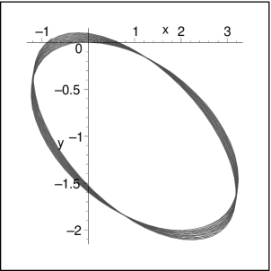
Figure 1:

The particle’s trajectory projected onto transverse plane for $\frac{\alpha}{m}=\frac{\beta}{m}=2,\omega=1,h=0.001$ and $0\leq\tau\leq 100000$.

acknowledgment

I would like to thank the research council of the Payame Noor University for partial financial support.

appendix

In this appendix we gather some linearized solutions for the particles trajectory and spin. Putting $\zeta(0)=\dot{\zeta}(0)=0$, Eq. (35) reduces to first order in $h$ to

$$\zeta(\tau) = \frac{\bar{c}}{2m}+\frac{ihc}{2m}e^{i\omega\tau}-\frac{ihc}{2m}e^{-i\omega\tau}-\frac{{\bar{c}}+2ic}{4m}e^{ih\omega\tau}+\frac{2ic-\bar{c}}{4m}e^{-ih\omega\tau},$$ (57)

or equivalently

$$x(\tau) = \frac{\alpha}{2m}-\frac{h\alpha}{m}\sin(\omega\tau)+\frac{\alpha}{m}\sin(h\omega\tau)-\frac{\alpha}{2m}\cos(h\omega\tau),$$ (58)

$$y(\tau) = \frac{\beta}{2m}+\frac{h\beta}{m}\sin(\omega\tau)-\frac{\beta}{m}\sin(h\omega\tau)-\frac{\beta}{2m}\cos(h\omega\tau).$$ (59)

Thus from Eq. (29) we obtain (with $v(0)=0$)

$$v(\tau) = \tau+O(h^{2}).$$ (60)

Eq. (30) and (58)-(60) determine the particle’s trajectory. From Eq. (22) we obtain

$$s^{34}(\tau) = \gamma$$ (61)

where $\gamma$ is a constant of integration.

We may now put Eqs. (31)-(32) and (61) into (23)-(25) to find the other components of $s^{\mu\nu}$. The results may be fed into (13) (with $\epsilon^{1234}=+1$) to give $s^{\mu}$

$$s^{1}(\tau) = \frac{2h\omega}{m}\alpha\beta(1-\cos(\omega\tau))-\gamma,$$ (62)

$$s^{2}(\tau) = \frac{2h\omega}{m}\alpha\beta(1-\cos(\omega\tau))+\gamma,$$ (63)

$$s^{3}(\tau) = \beta-\frac{h\omega}{m}\alpha\gamma(1-\cos(\omega\tau)),$$ (64)

$$s^{4}(\tau) = -\alpha-\frac{h\omega}{m}\beta\gamma(1-\cos(\omega\tau)),.$$ (65)

References

• [1] M. Mohseni and H. R. Sepangi, Class. Quantum Grav. 17 (2000), 4615.
• [2] R. H. Rietdijk and J. W. von Holten, Class. Quantum Grav. 7 (1990), 247.
• [3] A. Barducci, R. Casalbuoni, and L. Lussana, Nucl. Phys. B124 (1977), 521
• [4] G. W. Gibbons, R. H. Rietdijk, and J. W. van Holten, Nucl. Phys. B404 (1993), 42.
• [5] R. H. Rietdijk and J. W. van Holten, Class. Quantum Grav. 10 (1993), 575.
• [6] M. H. Ali and M. Ahmed, Ann. Phys. (NY), 282 (2000), 157.
• [7] J. W. van Holten, in Proc. Sem. Math. Sstructures in Field Theories 1986-87, ed. E. A. de Kerf and H. G. J. Pijls (CWI Syllabus Vol. 26), 109.
• [8] J. W. van Holten, preprint hep-th/0201083.
• [9] M. Mohseni, R. W. Tucker, and C. Wang, in ”Proceedings of 9th Marcel Grossmann meeting”, to appear
• [10] M. Mohseni, R. W. Tucker, and C. Wang , Class. Quantum Grav. 18 (2001), 3007.
• [11] S. Kessari, D. Singh, R. W. Tucker, and C. Wang, preprint gr-qc/0203038
• [12] M. Mohseni, unpublished.
• [13] D. Kramer, H. Stephani, M. McCollum , and E. Herlt, ”Exact solutions of Einstein’s field equations”, Cambridge university press, (1980).
• [14] G. W. Dixon, Nuovo Cimento 34 (1964) 317.