Wormholes supported by the kink-like configuration of a scalar field

Abstract

We study the problem of existence of static spherically symmetric wormholes supported by the kink-like configuration of a scalar field. With this aim we consider a self-consistent, real, nonlinear, nonminimally coupled scalar field $\phi$ in general relativity with the symmetry-breaking potential $V(\phi)$ possessing two minima. We classify all possible field configurations ruling out those of them for which wormhole solutions are impossible. Field configurations admitting wormholes are investigated numerically. Such the configurations represent a spherical domain wall localized near the wormhole throat.

curved spacetime

I Introduction

One of the most central feature of wormhole physics is the fact that traversable wormholes as solutions to the Einstein equations are accompanied by unavoidable violations of many of the energy conditions, i.e., the matter threading the wormhole’s throat has to be possessed of “exotic” properties MT (see also Ref. HV ). The known classical matter does satisfy the usual energy conditions, hence wormholes, if they exist, should arise as solutions of general relativity and “unusal” and/or quantum matter. One approach is to regard wormholes as semiclassical in nature Su92 ; HPS ; PS ; Pop01 ; THS ; Od ; Kha . In particular, self-consistent semiclassical wormhole solutions have been found numerically in Refs. Su92 ; HPS . Another way is to consider “exotic” field theories or theories based on various modifications of general relativity. For example, wormholes supported by ghost fields or fields with a negative sign kinetic term was discussed in Refs. Bron73 ; Kodama ; HKL ; Hayward ; Armen , and wormhole solutions in the Brans-Dicke theory was studied in Refs. Agnese ; Nandi ; Anch ; HK . It is worth to note that most of these works can be considered with the unified point of view as dealing with the scalar-tensor theory (STT) of gravity Bron73 ; Bron1 ; BS ; Bron-CC1 ; Bron-CC2 . The general STT action is given by

$$S=\int d^{4}x\sqrt{-g}\left\{\frac{1}{8\pi}f(\phi)R-h(\phi)g^{\mu\nu}\phi_{,\mu}\phi_{,\nu}-2V(\phi)\right\},$$ (1.1)

where $g_{\mu\nu}$ is a metric, $g=\det(g_{\mu\nu})$, $R$ is the scalar curvature, $\phi$ is a scalar field, $f$ and $h$ are certain functions of $\phi$, varying from theory to theory, and $V(\phi)$ is a potential. The particular choice $h(\phi)\equiv-1$ in the action 1.1 leads to the class of theories with the negative kinetic term. The Brans-Dicke theory BD , described in the Jordan frame, corresponds to the following case:

$$f(\phi)=\phi,\quad h(\phi)=\frac{\omega}{\phi}\,;\quad\omega={\rm const}\not=\frac{3}{2}.$$ (1.2)

A “less exotic” theory is represented by the nonminimally coupled scalar field in general relativity with the functions

$$f(\phi)=1-8\pi\xi\phi^{2},\quad h(\phi)\equiv 1;\quad\xi={\rm const}.$$ (1.3)

It turns out that such the theory also admits wormhole solutions. For the case $V=0$ (massless scalar field) the static spherically symmetric wormhole solutions was found in Ref. Bron73 (and recently discussed in Ref. BV1 ) for conformal coupling, $\xi=1/6$, and in Ref. BV2 for any $\xi>0$. It is important that more recent investigation BG has shown that such the solutions, obtained for the theory 1.1, 1.3 with $V=0$, are unstable under spherically symmetric perturbations.

In this paper we study the problem of existence of wormhole solutions in the theory 1.1, 1.3 with the symmetry-breaking potential $V(\phi)$ possessing two minima. The motivation for such the consideration is at least twofold. First, there exists a common opinion that the spacetime of the early Universe may have the nontrivial topological structure called the spacetime foam. Such the “foamy” structure consists of objects like primordial wormholes which can survive in the course of cosmological evolution. As is well known the evolution of the early Universe is accompanied by symmetry-breaking phase transitions which may have generated nontrivial topologically stable field configurations (topological defects) such as domain walls, strings, or monopoles Kibble ; VSh . The interplay of gravity and nonlinear field matter leads to a wealth of interesting phenomena remark . In particular, a static spherically symmetric wormhole solution was found in the framework of the so-called $\lambda\phi^{4}$ model with the “abnormal” negative-sign kinetic term Kodama . Also, the properties of spherical domain walls in a wormhole spacetime have been studied in Ref. Su01 . The second important reason, justifying our interest in this problem, is the following: A scalar field theory with the symmetry-breaking potential with two minima admits the existence of topologically stable kink-like configurations (domain walls or interfaces), such that the scalar field $\phi$ varies from $\phi_{1}$ to $\phi_{2}$, where $\phi_{1,2}$ are vacuum states corresponding to the minima of potential. Suppose that there exists a static spherically symmetric wormhole solution supported by the kink-like configuration of the scalar field, i.e., the spacetime geometry represents two asymptotically flat regions (universies) connected by a throat, and the scalar field $\phi$ is equal to $\phi_{1}$ in one asymptotically flat region and $\phi_{2}$ in the other one, varying substantially within a region near the throat. Such the configuration, if it exists, should be topologically stable, and so one may expect that it would also be stable under spherically symmetric perturbations.

This article is organized as follows: In the section II we derive the basic field equations. In the section III we, analyzing the field equations, represent some general analytical results and theorems and classify all possible field configurations ruling out that of them for which wormhole solutions are impossible. The particular model of the scalar field with the symmetry-breaking potential is considered in the section IV. We analyze this model numerically and obtain solutions describing wormholes supported by the kink-like configuration of the scalar field. Some discussion is given in the section V.

II Field equations

Consider a real scalar field $\phi$ nonminimally coupled to general relativity. Its action is given by Eqs. 1.1, 1.3. Varying the action 1.1 gives the equation of motion of the scalar field

$$\nabla^{\alpha}\nabla_{\alpha}\phi-V_{\phi}-\xi R\phi=0,$$ (2.4)

and the Einstein equations

$$G_{\mu\nu}=8\pi T_{\mu\nu},$$ (2.5)

where $V_{\phi}\equiv dV/d\phi$, $G_{\mu\nu}$ is the Einstein tensor, and the stress-energy tensor is given by

$$T_{\mu\nu} = \nabla_{\mu}\phi\nabla_{\nu}\phi-\frac{1}{2}g_{\mu\nu}(\nabla\phi)^{2}-g_{\mu\nu}V(\phi)$$

$$+\xi\phi^{2}G_{\mu\nu}-2\xi\left[\nabla_{\mu}(\phi\nabla_{\nu}\phi)-g_{\mu\nu}\nabla^{\lambda}(\phi\nabla_{\lambda}\phi)\right].$$

By grouping all the dependence on $G_{\mu\nu}$ on the left-hand side of the Einstein equations we can rewrite them in the equivalent form

$$G_{\mu\nu}=8\pi T_{\mu\nu}^{\rm(eff)}$$ (2.7)

where

$$T_{\mu\nu}^{\rm(eff)} = \frac{1}{1-8\pi\xi\phi^{2}}\left[\nabla_{\mu}\phi\nabla_{\nu}\phi-\frac{1}{2}g_{\mu\nu}(\nabla\phi)^{2}-g_{\mu\nu}V(\phi)-2\xi\left(\nabla_{\mu}(\phi\nabla_{\nu}\phi)-g_{\mu\nu}\nabla^{\lambda}(\phi\nabla_{\lambda}\phi)\right)\right].$$

is an effective stress-energy tensor. $T_{\mu\nu}$ and $T_{\mu\nu}^{\rm(eff)}$ are related as

$$T_{\mu\nu}^{\rm(eff)}=\frac{T_{\mu\nu}-\xi\phi^{2}G_{\mu\nu}}{1-8\pi\xi\phi^{2}}.$$ (2.9)

For a static, spherically symmetric configuration, the metric can be taken in the form Bron1 ; BS

$$ds^{2}=-A(\rho)dt^{2}+\frac{d\rho^{2}}{A(\rho)}+r^{2}(\rho)(d\theta^{2}+\sin^{2}\theta\,d\varphi^{2}),$$ (2.10)

and $\phi=\phi(\rho)$. The nontrivial equations of the system 2.7 are

$$2A\frac{r^{\prime\prime}}{r}+A^{\prime}\frac{r^{\prime}}{r}+A\frac{{r^{\prime}}^{2}}{r^{2}}-\frac{1}{r^{2}} = -8\pi\varepsilon^{\rm(eff)},$$ (2.11a)

$$A^{\prime}\frac{r^{\prime}}{r}+A\frac{{r^{\prime}}^{2}}{r^{2}}-\frac{1}{r^{2}} = 8\pi\sigma^{\rm(eff)},$$ (2.11b)

$$\frac{1}{2}A^{\prime\prime}+A^{\prime}\frac{r^{\prime}}{r}+A\frac{r^{\prime\prime}}{r} = 8\pi p^{\rm(eff)},$$ (2.11c)

where the prime denotes $d/d\rho$, and $\varepsilon^{\rm(eff)}=-{T_{0}^{0}}^{\rm(eff)}$ is the effective energy density, $\sigma^{\rm(eff)}={T_{1}^{1}}^{\rm(eff)}$ is the effective radial pressure, and $p^{\rm(eff)}={T_{2}^{2}}^{\rm(eff)}={T_{3}^{3}}^{\rm(eff)}$ is the effective transverse pressure. Using Eq. II we find

$$\varepsilon^{\rm(eff)} = \frac{1}{1-8\pi\xi\phi^{2}}\left[\frac{1}{2}A{\phi^{\prime}}^{2}+V(\phi)-\xi A(\phi^{2})^{\prime\prime}-\xi(\phi^{2})^{\prime}\left(\frac{1}{2}A^{\prime}+2A\frac{r^{\prime}}{r}\right)\right],$$ (2.12)

$$\sigma^{\rm(eff)} = \frac{1}{1-8\pi\xi\phi^{2}}\left[\frac{1}{2}A{\phi^{\prime}}^{2}-V(\phi)+\xi(\phi^{2})^{\prime}\left(\frac{1}{2}A^{\prime}+2A\frac{r^{\prime}}{r}\right)\right],$$ (2.13)

$$p^{\rm(eff)} = \frac{1}{1-8\pi\xi\phi^{2}}\left[-\frac{1}{2}A{\phi^{\prime}}^{2}-V(\phi)+\xi A(\phi^{2})^{\prime\prime}+\xi(\phi^{2})^{\prime}\left(A^{\prime}+A\frac{r^{\prime}}{r}\right)\right].$$ (2.14)

Only two of three equations of the system 2.11 are independent: Eq. 2.11b is a first integral of the others. Certain combinations of Eqs. 2.11 give two independent equations in the following form: 

$$2\frac{r^{\prime\prime}}{r} = -\frac{8\pi}{1-8\pi\xi\phi^{2}}\left[{\phi^{\prime}}^{2}-\xi(\phi^{2})^{\prime\prime}\right],$$ (2.15)

$$A(r^{2})^{\prime\prime}-A^{\prime\prime}r^{2}-2 = -\frac{8\pi\xi(\phi^{2})^{\prime}}{1-8\pi\xi\phi^{2}}r^{4}\left(\frac{A}{r^{2}}\right)^{\prime}.$$ (2.16)

Note that the potential $V(\phi)$ does not enter into the above expressions. The equation of motion of the scalar field, Eq. 2.4, in the metric 2.10 reads

$$(r^{2}A\phi^{\prime})^{\prime}-r^{2}V_{\phi}-\xi r^{2}R\phi=0,$$ (2.17)

with

$$R=-A^{\prime\prime}-4A^{\prime}\frac{r^{\prime}}{r}-4A\frac{r^{\prime\prime}}{r}-2A\frac{{r^{\prime}}^{2}}{r^{2}}+\frac{2}{r^{2}}.$$ (2.18)

Given the potential $V(\phi)$ Eqs. 2.17, 2.15, and 2.16 are a determined set of equations for the unknowns $r$, $A$, and $\phi$. Note that in the case $\xi=0$ this system reproduces the equations given in Ref. Bron1 .

It is worth to emphasize that the choice of a general spherically symmetric metric in the form 2.10 is convenient for a number of reasons Bron1 ; BS . In particular, as was shown in Refs. Bron1 ; BS for the minimal coupled scalar field, the equation 2.16 can be integrated. Fortunately, in the general case with arbitrary $\xi$ one can integrate Eq. 2.16 as well. Really, using a new denotation

$$B=r^{4}\left(\frac{A}{r^{2}}\right)^{\prime},$$ (2.19)

we can rewrite Eq. 2.16 as follows

$$(fB)^{\prime}=-2f.$$ (2.20)

Integrating the last equation gives

$$B=-\frac{2}{f}\left(\int^{\rho}f(\zeta)d\zeta-c_{1}\right),$$ (2.21)

where $c_{1}$ is an integration constant. Taking into account Eq. 2.19 and integrating once more we obtain

$$A=r^{2}\left(c_{2}+\int^{\rho}\frac{B(\zeta)}{r^{4}(\zeta)}d\zeta\right),$$ (2.22)

where $c_{2}$ is another integration constant.

III Wormholes and the kink-like configuration of a scalar field: Some general results

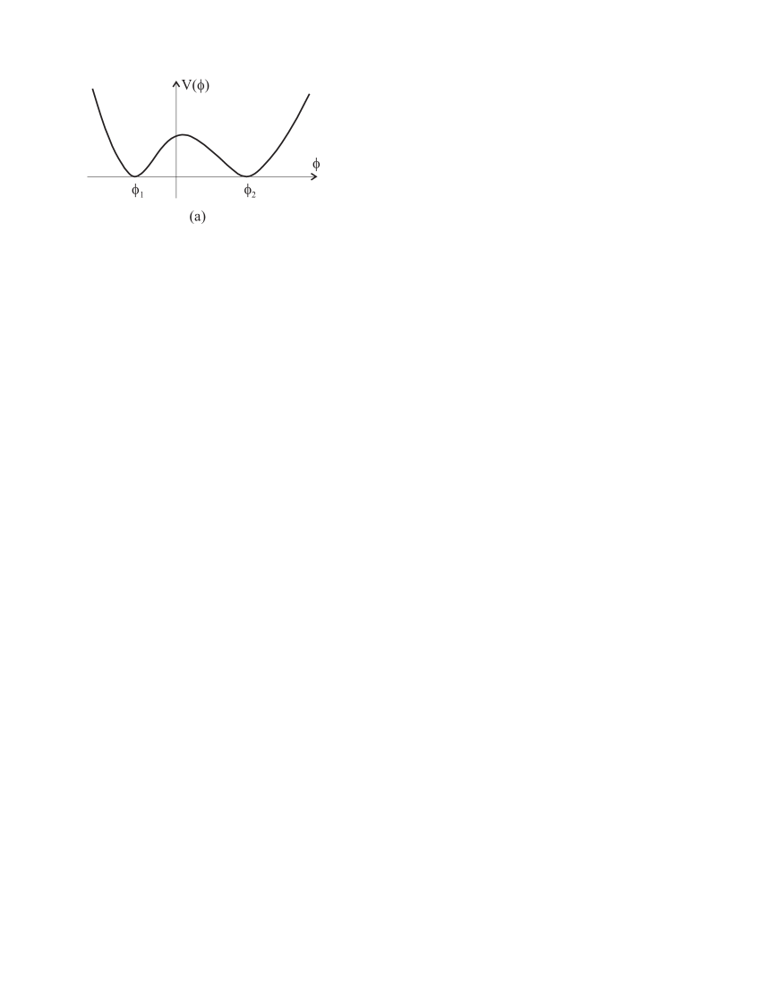
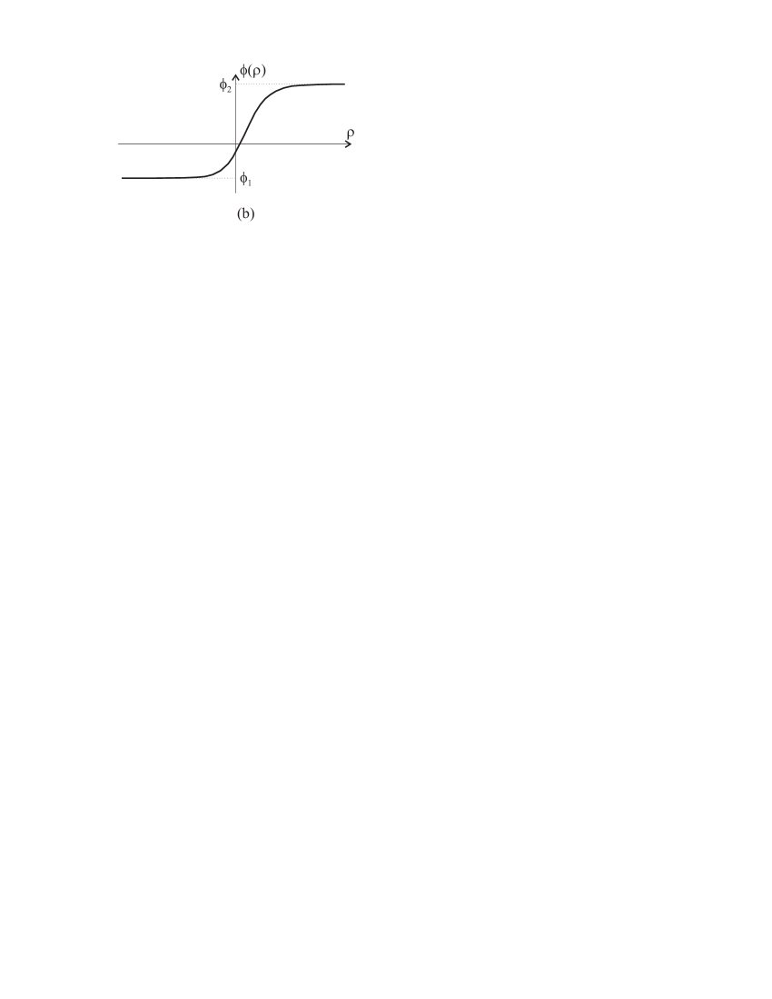
Figure 1: (a) A general form of the symmetry-breaking positive-definite potential $V(\phi)$. Two minima correspond to two vacuum states of the scalar field; (b) The kink-like configuration of the scalar field. The scalar field varies from $\phi_{1}$ to $\phi_{2}$.

Consider a symmetry-breaking potential $V(\phi)$ with two minima at $\phi_{1}$ and $\phi_{2}$, respectively (see Fig.1a). We will assume that the potential is positively definite, $V(\phi)\geq 0$, and $V(\phi_{1})=V(\phi_{2})=0$, so that the values $\phi_{1}$ and $\phi_{2}$ correspond to the real vacuum of the scalar field.

We will search such solutions of Eqs. 2.17, 2.15, 2.16 which describe a static spherically symmetric traversable wormhole. This means that the metric functions $r(\rho)$ and $A(\rho)$ should possess the following properties (for details, see Ref. VisserBook ):

• $r(\rho)$ has a global minimum, say $r_{*}=r(\rho_{*})$, such that $r_{*}>0$; the point $\rho_{*}$ is the wormhole’s throat, and $r_{*}$ is the throat’s radius;

• $A(\rho)$ is everywhere positive, i.e. no event horizons exist in the spacetime;

• the spacetime geometry is regular, i.e. no singularities exist;

• $r(\rho)\to|\rho|$ and $A(\rho)\to{\rm const}$ at $|\rho|\to\infty$; this guarantees an existence of two asymptotically flat regions ${\cal R}_{\pm}:\ \rho\to\pm\infty$ connected by the throat.

As for the scalar field, we will suppose that it has a kink-like configuration with nontrivial topological boundary conditions, i.e., the scalar field is in one of the vacuum states, say $\phi=\phi_{1}$, in the asymptotically flat region ${\cal R}_{-}$, and it is in the other vacuum state, $\phi=\phi_{2}$, in ${\cal R}_{+}$; in the intermediate region $-\infty<\rho<\infty$ the field smoothly varies from $\phi_{1}$ to $\phi_{2}$ (see Fig.1b). Such the field configuration represents a spherical domain wall (interface) localized near the wormhole throat.

The theory described by the set of nonlinear second-order differential equations 2.15, 2.16 and 2.17 is rather complicated and it is necessary to use numerical methods for its complete study. Until numerical calculations we will analyze some general properties of the theory. The crucial role in our analysis will play the function $f(\phi)=1-8\pi\xi\phi^{2}$ whose behavior is determined by the values $\xi$, $\phi_{1}$ and $\phi_{2}$. Let us consider various cases:

1. $\xi=0$. In this case the action 1.1 describes the theory of a scalar field minimally coupled to general relativity. No-go theorems proven in Refs. Bron1 ; BS state, in particular, that wormhole solutions are not admitted in this case. It will be useful to reproduce here the proof of this statement: For $\xi=0$ Eq. 2.15 reduces to

$$2\frac{r^{\prime\prime}}{r}=-8\pi{\phi^{\prime}}^{2}.$$ (3.23)

Since $r(\rho)\geq 0$ by its geometric meaning, the last equation gives $r^{\prime\prime}\leq 0$, which rules out an existence of regular minima of $r(\rho)$, and hence an existence of wormhole solutions.

2. $\xi<0$. In this case the function $f^{-1}=(1-8\pi\xi\phi^{2})^{-1}$ is regular (i.e., finite, smooth, and positive) in the whole range of $\rho$, and so we can assert that a wormhole solution is impossible. The proof of this assertion is given in Refs. Bron-CC1 ; Bron-CC2 , where the reader can find details. Here we shortly reproduce main points of that proof. With this purpose we introduce a new metric $\bar{g}_{\mu\nu}$ and a new scalar field $\psi$ using Wagoner’s Wagoner conformal transformation

$$g_{\mu\nu}=F(\psi)\bar{g}_{\mu\nu},\quad F=\frac{1}{f},$$

$$\frac{d\psi}{d\phi}=\pm\frac{\sqrt{|l(\phi)|}}{f(\phi)},\quad l(\phi)=f+\frac{3}{2}\left(\frac{df}{d\phi}\right)^{2}.$$ (3.24)

Now one can write the action 1.1 as follows:

$$S=\int d^{4}x\sqrt{-\bar{g}}\left[\frac{1}{8\pi}\overline{R}-(\partial\psi)^{2}-2\overline{V}(\psi)\right],$$ (3.25)

where

$$\overline{V}(\psi)=\frac{1}{f^{2}}V(\phi).$$ (3.26)

One can see that the transformation 3.24 removes the nonminimal coupling expressed in the $\phi$-dependent coefficient before $R$ in Eq. 1.1, so that Eq. 3.25 represents the action of the scalar field $\psi$ minimally coupled to general relativity. Because the conformal factor $F=f^{-1}$ is regular the theories 1.1 and 3.25 are conformally equivalent, in particular, the global structure of spacetimes $M[g]$ and $\overline{M}[\bar{g}]$ is the same. No-go theorems proven in Refs. Bron1 ; BS state that the theory 3.25 does not admit wormhole solutions. Hence we should conclude that wormholes are also impossible in the theory 3.25 with $\xi<0$.

3. $\xi>0$.

3a: $|\phi_{1}|<(8\pi\xi)^{-1/2}$ and $|\phi_{2}|<(8\pi\xi)^{-1/2}$ (i.e., $|\phi|$ is small);

3b: $|\phi_{1}|>(8\pi\xi)^{-1/2}$, $|\phi_{2}|>(8\pi\xi)^{-1/2}$ (i.e., $|\phi|$ is large), and $\phi_{1}$, $\phi_{2}$ have the same sign (both $\phi_{1}$ and $\phi_{2}$ are positive or negative).

Since, for the cases 3a and 3b, the conformal factor $F=f^{-1}=(1-8\pi\xi\phi^{2})^{-1}$ is regular in the whole range of $\rho$, we can again assert that a wormhole solution is impossible.

3c: $|\phi_{1}|>(8\pi\xi)^{-1/2}$, $|\phi_{2}|>(8\pi\xi)^{-1/2}$, and $\phi_{1}$, $\phi_{2}$ have opposite signs (say $\phi_{1}<-(8\pi\xi)^{-1/2}$ and $\phi_{2}>(8\pi\xi)^{-1/2}$).

The case 3c represents the kink-like configuration such that the scalar field smoothly interpolates between two super-Planckian values $\phi_{1}<-(8\pi\xi)^{-1/2}$ and $\phi_{2}>(8\pi\xi)^{-1/2}$. In this case the function $f=1-8\pi\xi\phi^{2}$ becomes to be equal to zero at two points $\rho_{1}$ and $\rho_{2}$, where $|\phi(\rho_{1})|=|\phi(\rho_{2})|=\phi_{0}=(8\pi\xi)^{-1/2}$, and hence the conformal factor $F=f^{-1}=(1-8\pi\xi\phi^{2})^{-1}$ turns out to be singular at these points. Referring to Bron-CC2 , we say that the spheres $\rho=\rho_{1}$ and $\rho=\rho_{2}$ are transition surfaces, $S_{\rm trans}$. Note that, though $F$ is singular on $S_{\rm trans}$, the metric $g_{\mu\nu}$ can still be regular if the metric $\bar{g}_{\mu\nu}$ specified by the conformal transformation 3.24 has an appropriate behavior on $S_{\rm trans}$. Bronnikov Bron-CC1 ; Bron-CC2 called such the situation a conformal continuation from $\overline{M}[\bar{g}]$ into $M[g]$ and obtained some of properties of conformally continued solutions. In particular, he pointed out that the no-go theorems Bron1 ; BS forbidding wormhole solutions in the theory 3.25 cannot be directly transferred to the theory 1.1 if the conformal factor $F$ vanishes or has a singular behavior at some values of $\rho$. However, there are still no general results allowing to assert without specifying $F$ either wormholes are admitted in the theory 1.1 or not. To solve this problem in the case 3c we prove the following theorem.

Theorem 1. The field equations 2.15, 2.16, and 2.17 of the theory 1.1 do not admit regular  solutions where $\phi$ has the kink-like configuration such that $\phi(\rho)$ is at least a $C^{2}$-smooth function monotonically increasing from $\phi_{1}<-(8\pi\xi)^{-1/2}$ to $\phi_{2}>(8\pi\xi)^{-1/2}$ while $\rho$ runs from $-\infty$ to $\infty$.

Proof. Due to the theorem’s formulation the function $f(\rho)=1-8\pi\xi\phi^{2}(\rho)$ turns into zero only  at two points, say $\rho_{1}$ and $\rho_{2}$, so that $f(\rho_{1})=f(\rho_{2})=0$, and otherwise $f(\rho)\not=0$. Consider Eq. 2.16. One can write it in the form 2.20 and then, integrating, in the form 2.21. Rewrite Eq. 2.21 as follows:

$$r^{4}\left(\frac{A}{r^{2}}\right)^{\prime}=-2\frac{h}{h^{\prime}},$$ (3.27)

where $h(\rho)$ is a primitive function for $f(\rho)$, so that $h^{\prime}=f$. Note that the denominator in the right-hand side of Eq. 3.27 is equal to zero at the points $\rho_{1}$ and $\rho_{2}$, $h^{\prime}(\rho_{1})=h^{\prime}(\rho_{2})=0$. Suppose that the nominator becomes also to be equal to zero at these points, $h(\rho_{1})=h(\rho_{2})=0$, so that the ratio $h/h^{\prime}$ remains to be regular. Because $h$ is a smooth function being equal to zero at the boundaries of the interval $(\rho_{1},\rho_{2})$, there exists a point within the interval, $\rho_{1}<\rho_{*}<\rho_{2}$, where $h$ has an extremum, so that $h^{\prime}(\rho_{*})=0$. Hence $f(\rho_{*})=0$. We have obtained a contradiction which proves the theorem.

An immediate corollary of the theorem 1 is that the theory 1.1 does not admit wormholes supported by the field configuration 3c. Note also that the proof of the theorem rests actually on a feature of the function $f(\rho)$ possessing exactly two zeros. It is obvious that the theorem can be extended to cases when $f(\rho)$ has an even number of zeros.

3d: $|\phi_{1}|<(8\pi\xi)^{-1/2}$, $|\phi_{2}|>(8\pi\xi)^{-1/2}$.

The case 3d represents the kink-like configuration such that the scalar field varies from a small value $|\phi_{1}|<(8\pi\xi)^{-1/2}$ to a large value $\phi_{2}>(8\pi\xi)^{-1/2}$. In this case there is just one and only point, say $\rho_{0}$, where $|\phi(\rho_{0})|=\phi_{0}=(8\pi\xi)^{-1/2}$, and hence the conformal factor $F=f^{-1}=(1-8\pi\xi\phi^{2})^{-1}$ turns out to be singular at this point. The theorem 1 proven for the configuration 3c does not work now, and one may suppose that wormhole solutions supported by the field configuration 3d could exist in the theory 1.1. Indeed, for the potential $V(\phi)$ being equal to zero, such the solutions was found for the first time by Bronnikov Bron73 (see also Ref. BV1 ) for conformal coupling, $\xi=1/6$, and more recently by Barceló and Visser BV2 for any $\xi>0$.

In the next section we will obtain a wormhole solution for the symmetry-breaking potential $V(\phi)$.

IV Wormhole solution

IV.1 Model and analysis of boundary conditions

Consider a ‘toy’ symmetry-breaking potential

$$V(\phi)=\frac{\lambda}{4}\left[(\phi-\bar{\phi})^{2}-\frac{m^{2}}{\lambda}\right]^{2},$$ (4.28)

where $\lambda>0$, $m>0$, and $\bar{\phi}$ are some constants. The minima of the potential 4.28 correspond to

$$\phi_{1}=-\frac{m}{\sqrt{\lambda}}+\bar{\phi},\quad\phi_{2}=\frac{m}{\sqrt{\lambda}}+\bar{\phi}.$$ (4.29)

Note that the configuration 3d is only possible provided $\bar{\phi}\not=0$.

At present it will be convenient to introduce new dimensionless variables and quantities

$$x=m\rho,\quad\tilde{r}(x)=mr(\rho),\quad\eta(x)=\frac{\phi(\rho)}{\kappa},$$

$$\bar{\eta}=\frac{\bar{\phi}}{\kappa},\quad\bar{\eta}_{1}=-1+\bar{\eta},\quad\bar{\eta}_{2}=1+\bar{\eta},\quad\kappa=\frac{m}{\sqrt{\lambda}}.$$ (4.30)

Taking into account Eq. 4.28 we rewrite the field equations 2.15, 2.16 and 2.17 in the dimensionless form:

$$2\frac{r^{\prime\prime}}{r}=-\frac{8\pi\kappa^{2}}{1-8\pi\xi\kappa^{2}\eta^{2}}\left[{\eta^{\prime}}^{2}-\xi(\eta^{2})^{\prime\prime}\right],$$ (4.31)

$$A(r^{2})^{\prime\prime}-A^{\prime\prime}r^{2}-2=-\frac{8\pi\xi\kappa^{2}(\eta^{2})^{\prime}}{1-8\pi\xi\kappa^{2}\eta^{2}}\,r^{4}\left(\frac{A}{r^{2}}\right)^{\prime},$$ (4.32)

$$(r^{2}A\eta^{\prime})^{\prime}-\xi r^{2}R(x)\eta-r^{2}(\eta-\bar{\eta})\left[(\eta-\bar{\eta})^{2}-1\right]=0,$$ (4.33)

with

$$R(x)=-A^{\prime\prime}-4A^{\prime}\frac{r^{\prime}}{r}-4A\frac{r^{\prime\prime}}{r}-2A\frac{{r^{\prime}}^{2}}{r^{2}}+\frac{2}{r^{2}},$$

where the prime denotes $d/dx$. (Notice: For short hereafter we drop a tilde over $\tilde{r}(x)$.) Resolve the last system in terms of the second derivatives $r^{\prime\prime}$, $A^{\prime\prime}$, and $\eta^{\prime\prime}$:

$$r^{\prime\prime} = \frac{r}{6\xi^{2}\eta^{2}+f}\left[-\frac{1}{2}{\eta^{\prime}}^{2}(1-2\xi)-\xi\eta\eta^{\prime}\left(2\frac{r^{\prime}}{r}+\frac{A^{\prime}}{A}\right)+\xi\frac{1}{A}\eta\Delta\eta(\Delta\eta^{2}-1)\right.$$ (4.34)

$$\left.-4\xi^{2}\eta^{2}\left(\frac{{r^{\prime}}^{2}}{r^{2}}+\frac{r^{\prime}A^{\prime}}{rA}-\frac{1}{r^{2}A}\right)+2\frac{\xi^{3}\eta^{3}\eta^{\prime}}{f}\left(2\frac{r^{\prime}}{r}-\frac{A^{\prime}}{A}\right)\right],$$

$$A^{\prime\prime} = \frac{A}{6\xi^{2}\eta^{2}+f}\left[-{\eta^{\prime}}^{2}(1-2\xi)+2f\left(\frac{{r^{\prime}}^{2}}{r^{2}}-\frac{1}{r^{2}A}\right)-8\xi\eta\eta^{\prime}\frac{r^{\prime}}{r}+2\xi\frac{1}{A}\eta\Delta\eta(\Delta\eta^{2}-1)\right.$$ (4.35)

$$\left.+4\xi^{2}\eta^{2}\left(\frac{{r^{\prime}}^{2}}{r^{2}}-2\frac{r^{\prime}A^{\prime}}{rA}-\frac{1}{r^{2}A}\right)-8\frac{\xi^{3}\eta^{3}\eta^{\prime}}{f}\left(2\frac{r^{\prime}}{r}-\frac{A^{\prime}}{A}\right)\right],$$

$$\eta^{\prime\prime} = \frac{1}{6\xi^{2}\eta^{2}+f}\left[-\eta^{\prime}f\left(2\frac{r^{\prime}}{r}+\frac{A^{\prime}}{A}\right)+\frac{f}{A}\Delta\eta(\Delta\eta^{2}-1)+3\xi\eta{\eta^{\prime}}^{2}(1-2\xi)\right.$$ (4.36)

$$\left.-4\xi f\eta\left(\frac{{r^{\prime}}^{2}}{r^{2}}+\frac{r^{\prime}A^{\prime}}{rA}-\frac{1}{r^{2}A}\right)+2\xi^{2}\eta^{2}\eta^{\prime}\left(2\frac{r^{\prime}}{r}-\frac{A^{\prime}}{A}\right)\right].$$

where

$$f=(8\pi\kappa)^{-2}(1-8\pi\xi\kappa^{2}\eta^{2}),\quad\Delta\eta\equiv\eta-\bar{\eta}.$$ (4.37)

Eqs. 4.34, 4.35 and 4.36 represent a system of three ordinary second-order differential equations which has a general solution depending, generally speaking, on six parameters.

Let us discuss the case of our interest. Suppose that there exists a point $x=x_{0}$ where $\eta(x_{0})=(8\pi\xi\kappa^{2})^{-1/2}$, so that $f(x_{0})=0$; without loss of generality we can assume that $x_{0}=0$. To ensure a regular behavior of the right-hand sides of Eqs. 4.34, 4.35 we should provide regularity of the term $\frac{1}{f}\left(2\frac{r^{\prime}}{r}-\frac{A^{\prime}}{A}\right)$ at $x=0$. Hence we obtain

$$2\frac{r_{0}^{\prime}}{r_{0}}-\frac{A_{0}^{\prime}}{A_{0}}=0,$$ (4.38)

where $r_{0}=r(0)$ and so forth. This formula determines a relation between the values of the functions $r(x)$ and $A(x)$ and their first derivatives at the point $x=0$. An additional relation can be obtained by using Eq. 2.11b which is the first-order differential equation and plays a role of the constraint for boundary conditions. At the point $x=0$ it gives

$$\frac{r_{0}^{\prime}}{r_{0}}=-\frac{\sqrt{8\pi}\,\kappa}{12\sqrt{\xi}\,\eta_{0}^{\prime}A_{0}}\left(A_{0}{\eta_{0}^{\prime}}^{2}-\frac{1}{2}(\Delta\eta^{2}-1)^{2}\right).$$ (4.39)

Now the solution for $r(x)$, $A(x)$ and $\eta(x)$ being regular in the vicinity of $x=0$ can be expanded in the series: 

$$r(x) = r_{0}+r_{0}^{\prime}x+\frac{1}{2}r_{0}^{\prime\prime}x^{2}+\dots\,,$$

$$A(x) = A_{0}+A_{0}^{\prime}x+\frac{1}{2}A_{0}^{\prime\prime}x^{2}+\dots\,,$$

$$\eta(x) = \frac{1}{\kappa\sqrt{8\pi\xi}}+\eta_{0}^{\prime}x+\frac{1}{2}\eta_{0}^{\prime\prime}x^{2}+\dots\,,$$ (4.40)

where only three coefficients, say $r_{0}$, $A_{0}$ and $\eta^{\prime}_{0}$, are independent parameters; the others can be found by using the relations 4.38 and 4.39 and Eqs. 4.34, 4.35 and 4.36.

It is necessary to stress that our analysis of boundary conditions is local and based on the demand of regularity of a solution at the critical point $x=0$ where the function $f(x)$ becomes to be equal to zero. However this analysis does not answer the question about an existence of a wormhole solution with the kink-like configuration of the scalar field. In the next subsection we will show that such the solutions do really exist.

IV.2 Numerical results

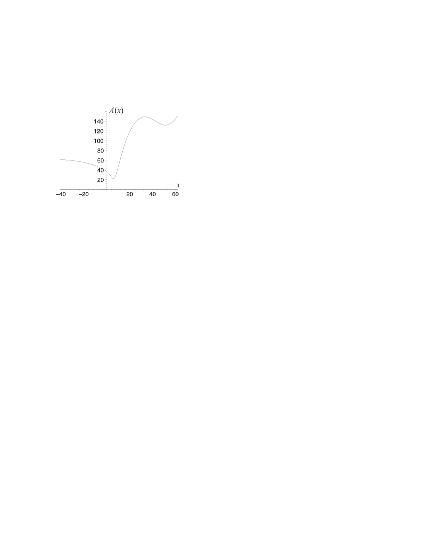
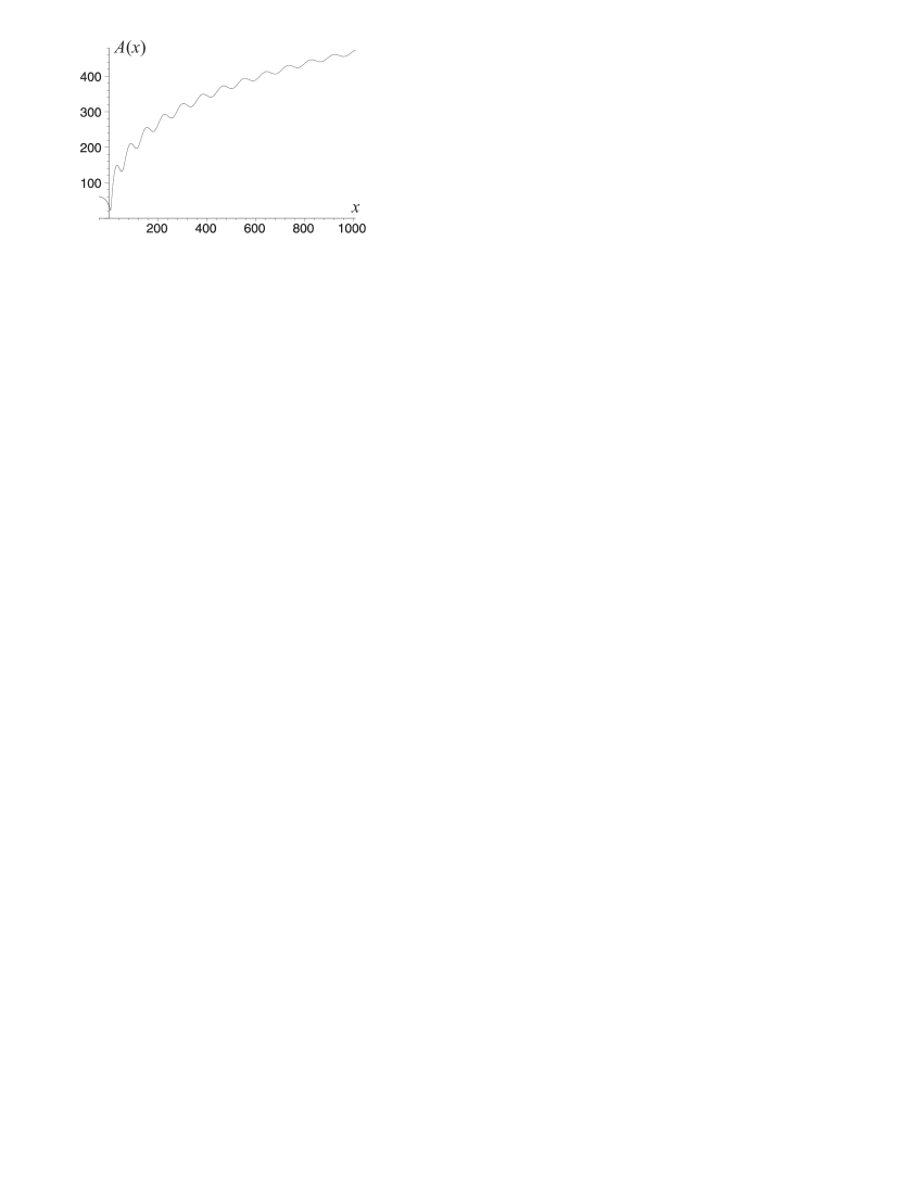
Figure 3: The numerical solution for $A(x)$ in the small and large scales; $\xi=1/6$, $\kappa=(8\pi)^{-1/2}$, $\bar{\eta}=(8\pi\xi\kappa^{2})^{-1/2}$.

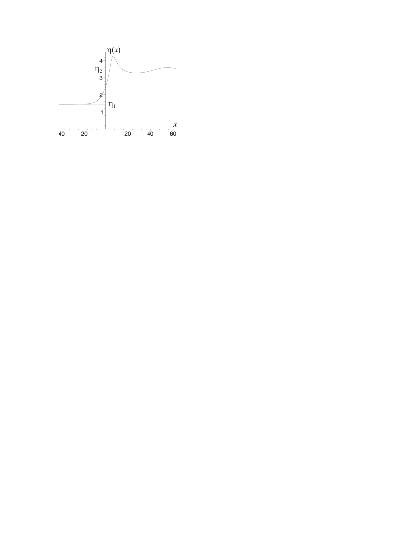
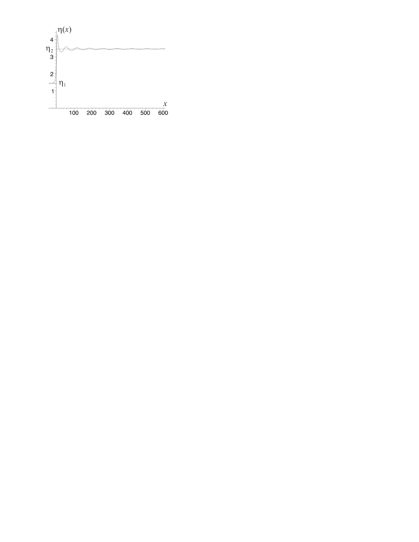
Figure 4: The kink-like configuration of the scalar field. The scalar field varies from $\eta_{1}=-1+(8\pi\xi\kappa^{2})^{-1/2}\approx 1.4495$ to $\eta_{2}=1+(8\pi\xi\kappa^{2})^{-1/2}\approx 3.4495$.

Taking into account the above analysis of boundary conditions we can solve the system of equations 4.34, 4.35 and 4.36 numerically. To perform this in practice we must specify the six parameters, where $\xi$, $\kappa$ and $\bar{\eta}$ are parameters of the model, and $r_{0}$, $A_{0}$ and $\eta^{\prime}_{0}$ are determining boundary conditions. Note that $\xi>0$ because the configuration 3d is of our interest, $\kappa>0$ by definition, and $r_{0}>0$ and $A_{0}>0$ by their geometric meaning. Though the local boundary condition analysis did not reveal any restrictions for $r_{0}$, $A_{0}$ and $\eta^{\prime}_{0}$, we may however suppose that topologically nontrivial solutions describing the kink-like configuration of the scalar field could only exist for some definite boundary conditions. In practical calculations we will fix two of three parameters $r_{0}$, $A_{0}$, $\eta^{\prime}_{0}$, tuning then a value of third parameter in order to obtain a solution with the kink-like field configuration. Some of numerical results are shown in Figs. 2-4 for the following set of parameters:

$$\xi=\frac{1}{6},\quad\kappa=\frac{1}{\sqrt{8\pi}},\quad\bar{\eta}=\frac{1}{\sqrt{8\pi\xi\kappa^{2}}},$$

$$r_{0}=1,\quad A_{0}=36.321278,\quad\eta^{\prime}_{0}=0.2.$$ (4.41)

Let us discuss the obtained results in details.

Graphs in Figs. 2-4 represent a numerical solution for the functions $r(x)$, $A(x)$ and $\eta(x)$, respectively. The form of graphs is nonsymmetric. The critical point $x=0$ separates two regions, $x<0$ and $x>0$, where behavior of the solutions is qualitatively different. In the region $x<0$ the functions $r(x)$, $A(x)$ and $\eta(x)$ are monotonic and have the following asymptotical behavior at $|x|\to\infty$:

$$r(x)\approx k_{1}|x|,\quad A(x)\approx a_{1}-\frac{b_{1}}{|x|},\quad\eta(x)\approx\eta_{1}.$$ (4.42)

where $k_{1}\approx 0.129$, $a_{1}\approx 70$, $b_{1}\approx 440$, and $\eta_{1}=-1+(8\pi\xi\kappa^{2})^{-1/2}\approx 1.4495$. While in the region $x>0$ they have an oscillating component superposed on a monotonic one, so that their asymptotics at $x\to\infty$ are

$$r(x)\approx k_{2}x+p\,\sin\omega x,\quad A(x)\approx a_{2}-\frac{b_{2}}{x}+q\,\sin\omega x,\quad\eta(x)\approx\eta_{2}+s\,\sin\omega x$$ (4.43)

where $k_{2}\approx 0.04$, $a_{2}\approx 770$, $b_{2}\approx 470000$, and $\eta_{2}=1+(8\pi\xi\kappa^{2})^{-1/2}\approx 3.4495$. Note that the amplitudes $p$, $q$, $s$ and the frequency $\omega$ are actually not constant, they depend on $x$ and are slowly decreasing while $x$ increases; within the interval from 0 to 1000 their values can be approximated as $p\approx 0.8$, $q\approx 10$, $\omega\approx 0.0769$.

It is necessary to emphasize that the solution obtained describes a wormhole with the kink-like configuration of the scalar field. Really, (i) the metric function $r(x)$ has the global minimum $r_{*}\approx 0.9484$ at the point $x_{*}\approx 3.52$, which is the wormhole’s throat; (ii) $r(x)$ approaches to $k|x|$ and $A(x)$ approaches to a constant in the asymptotical regions $|x|\to\infty$; this guarantees an existence of two asymptotically flat regions of the spacetime; (iii) the scalar field $\eta$ varies from one vacuum state $\eta_{1}$ at $x=-\infty$ to the other one $\eta_{2}$ at $x=\infty$; this represents the kink-like configuration. The distribution of the scalar field energy density $\varepsilon(x)$ is shown in Fig. 5. It is seen that it has a narrow peak at $x\approx 6.6$ near the throat; on the left of the peak the energy density is very fast decreasing; on the right the energy density is also fast decreasing making small oscillations around zero. Thus, the main part of the scalar field energy turns out to be concentrated in the narrow spherical region near the throat, and so we will call this region a spherical domain wall.

As is well known, traversable wormholes as solutions to the Einstein equations can only exist with exotic matter, for which many of the energy conditions should be violated MT (for details, see also Refs. BV2 ; HV ). Let us discuss our solution with this point of view. Consider the weak energy condition (WEC) which reads

$$G_{\mu\nu}v^{\mu}v^{\nu}=8\pi T^{\rm(eff)}_{\mu\nu}v^{\mu}v^{\nu}\geq 0,$$ (4.44)

where $v^{\mu}$ is properly normalized timelike vector, $v^{2}=-1$. For the static spherically symmetric configuration the WEC is equivalent to the positivity of the effective energy density,

$$\varepsilon^{\rm(eff)}\geq 0.$$ (4.45)

The graph for $\varepsilon^{\rm(eff)}$ is given in Fig. 6. It shows, as was expected, that the condition 4.45 is violated.

V Concluding remarks

So, we have obtained that the theory 1.1, 1.3 with the potential $V$ given by Eq. 4.28 admits solutions describing a wormhole supported by the kink-like configuration of the scalar field. Note that though the wormhole solution found numerically in the previous section was only given for particular values of parameters (see Eq. IV.2), our calculations have demonstrated that such solutions exist for a large scale of parameter’s values. Unfortunately, we have no reasonable analytical estimations allowing to impose more exact restrictions for a domain of admissible parameter’s values. Some rough restrictions for the parameters are dictated by the results of the section III, where it was shown that a wormhole solution can only exist for the configuration 3d. In particular, we have $\xi>0$. Note that there are no restrictions for the parameter $r_{0}$ which determines the throat’s radius. In our consideration we have specified $r_{0}=1$ and obtained the throat’s radius $r_{*}\approx 0.9484$. In practice of numerical calculations we have also used $r_{0}=10$ and $r_{0}=100$ with $r_{*}\approx 10$ and $r_{*}\approx 100$, respectively.

The important problem which needs to be discussed is the stability of solutions obtained. Recently, Bronnikov and Grinyok BG have shown that static spherically symmetric wormholes with the nonminimally coupled scalar field with $V=0$ are unstable under spherically symmetric perturbations. On the contrary, one may expect that wormholes supported by the scalar field with the symmetry-breaking potential $V$ would be stable because of the topological stability of the kink-like field configuration. Of course, this problem needs more serious consideration, and we intend to discuss it in a following publication.

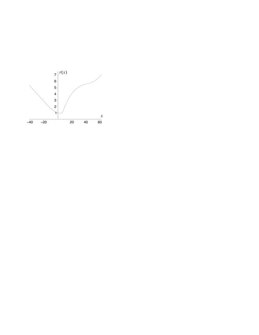
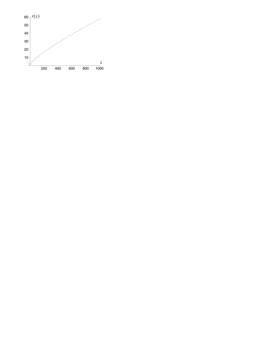
Figure 2: The numerical solution for $r(x)$ in the small and large scales; $\xi=1/6$, $\kappa=(8\pi)^{-1/2}$, $\bar{\eta}=(8\pi\xi\kappa^{2})^{-1/2}$.

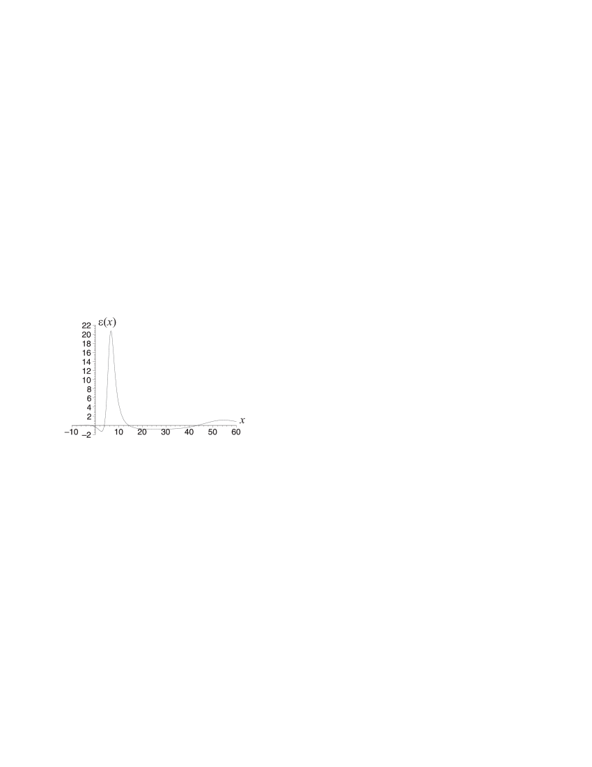
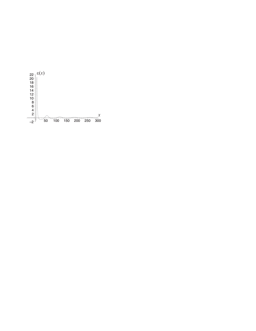
Figure 5: The graph of the energy density $\varepsilon(x)=-T_{0}^{0}$ in the small and large scales. The highest peak at $x\approx 6.6$ corresponds to a spherical domain wall.

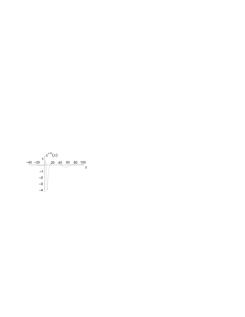
Figure 6: The graph of the effective energy density $\varepsilon^{\rm(eff)}(x)=-{T_{0}^{0}}^{\rm(eff)}$.

References

- (1) M. S. Morris, K. S. Thorne, Am. J. Phys. 56, 395 (1988),
- (2) D. Hochberg, M. Visser, Phys. Rev. D56, 4745 (1997),
- (3) S. V. Sushkov, Phys. Lett. A164, 33 (1992),
- (4) D. Hochberg, A. Popov, and S. V. Sushkov, Phys. Rev. Lett. 78, 2050 (1997),
- (5) A. A. Popov, S. V. Sushkov, Phys. Rev. D63, 044017 (2001),
- (6) A. A. Popov, Phys. Rev. D64, 104005 (2001),
- (7) B. E. Taylor, W. A. Hiscock, and P. R. Anderson, Phys. Rev. D55, 6116 (1997).
- (8) S. Nojiri, O. Obregon, S.D. Odintsov, K.E. Osetrin, Phys.Lett. B 449, 173 (1999); B 458, 19 (1999),
- (9) V. Khatsymovsky, Phys. Lett. B429, 254 (1998)
- (10) K. A. Bronnikov, Acta Physica Polonica B 4, 251 (1973),
- (11) T. Kodama, Phys. Rev. D18, 3529 (1978),
- (12) S. A. Hayward, S.-W. Kim, and H. Lee, Phys. Rev. D65, 064003 (2002),
- (13) S. A. Hayward, gr-qc/0202059,
- (14) C. Armendáriz-Picón, gr-qc/0201027.
- (15) A. Agnese and M. La Camera, Phys. Rev. D51, 2011 (1995),
- (16) K. K. Nandi, A. Islam, and J. Evans, Phys. Rev. D55, 2497 (1997),
- (17) L. A. Anchordoqui, S. Perez Bergliaffa, and D. F. Torres, Phys. Rev. D55, 5226 (1997),
- (18) F. He, S.-W. Kim, Phys. Rev. D65, 084022 (2002),
- (19) K. A. Bronnikov, Phys. Rev. D64, 064013 (2001),
- (20) K. A. Bronnikov, G. N. Shikin, gr-qc/0109027,
- (21) K. A. Bronnikov, Acta Physica Polonica B 32, 3571 (2001),
- (22) K. A. Bronnikov, gr-qc/0204001,
- (23) C. Brans, R. H. Dicke, Phys. Rev. 124, 925 (1961),
- (24) C. Barceló and M. Visser, Phys. Lett. 466B, 127 (1999),
- (25) C. Barceló and M. Visser, Class. Quantum Grav. 17, 3843 (2000),
- (26) K. A. Bronnikov, S. Grinyok, gr-qc/0201083; gr-qc/0205131.
- (27) T. W. Kibble, J. Phys. A 9, 1387 (1976).
- (28) A. Vilenkin and E. P. S. Shellard, Cosmic String and Other Topological Defects, Cambridge Monographs on Mathematical Physics (Cambridge University Press, Cambridge, 1994).
- (29) Among them are false vacuum black holes, cosmological and black hole solutions to the Einstein-Yang-Mills equations, and many others. However this field is very vast, and its review goes beyond the present paper.
- (30) S. V. Sushkov, Gravitation & Cosmology, 7, 197 (2001),
- (31) M. Visser, Lorentzian Wormholes: from Einstein to Hawking,(American Institute of Physics, Woodbury, 1995).
- (32) R. Wagoner, Phys. Rev. D1, 3209 (1970),