Sagnac Interferometer as a Speed-Meter-Type, Quantum-Nondemolition Gravitational-Wave Detector

Abstract

According to quantum measurement theory, “speed meters” — devices that measure the momentum, or speed, of free test masses — are immune to the standard quantum limit (SQL). It is shown that a Sagnac-interferometer gravitational-wave detector is a speed meter and therefore in principle it can beat the SQL by large amounts over a wide band of frequencies. It is shown, further, that, when one ignores optical losses, a signal-recycled Sagnac interferometer with Fabry-Perot arm cavities has precisely the same performance, for the same circulating light power, as the Michelson speed-meter interferometer recently invented and studied by P. Purdue and the author. The influence of optical losses is not studied, but it is plausible that they be fairly unimportant for the Sagnac, as for other speed meters. With squeezed vacuum (squeeze factor $e^{-2R}=0.1$) injected into its dark port, the recycled Sagnac can beat the SQL by a factor $\sqrt{10}\simeq 3$ over the frequency band $10{\rm Hz}\lesssim f\lesssim 150{\rm Hz}$ using the same circulating power $I_{c}\sim 820$ kW as is used by the (quantum limited) second-generation Advanced LIGO interferometers — if other noise sources are made sufficiently small. It is concluded that the Sagnac optical configuration, with signal recycling and squeezed-vacuum injection, is an attractive candidate for third-generation interferometric gravitational-wave detectors (LIGO-III and EURO).

I Introduction

After decades of planning and development, an array of large-scale laser interferometric gravitational-wave detectors (interferometers for short), consisting of the Laser Interferometer Gravitational-wave Observatory (LIGO), Virgo, GEO and TAMA GWarray , is gradually becoming operative, targeted at gravitational waves in the high-frequency band ($10$–$10^{3}\,\mathrm{Hz}$). Michelson-type laser interferometry is used in these detectors to monitor gravitational-wave-induced changes in the separations of mirror-endowed test masses. More specifically, a laser beam is split in two by a 50/50 beamsplitter, and the two beams are sent into the two arms (which may contain Fabry-Perot cavities) and then brought back together and interfered, yielding a signal that senses the difference of the two arm lengths. Although it is plausible that gravitational waves will be detected, for the first time in history, by these initial interferometers, a significant upgrade of them must probably be made before a rich program of observational gravitational-wave astrophysics can be carried out matureLIGO . In the planned upgrade of the LIGO interferometers (Advanced LIGO, tentatively scheduled to begin operations in $2008$ whitpaper ), the Michelson topology will still be used, as also is probably the case for Advanced LIGO’s international counterparts, for example the Japanese LCGT LCGT .

An alternative to the Michelson topology, the Sagnac topology, originally invented in 1913 SagnacOrig for rotation sensing, can also be used for gravitational-wave detection Drever ; Sagnac . In a Sagnac interferometer, as in a Michelson, a laser beam is split in two, but each of the two beams travels successively through both arms, though in the opposite order (in opposite directions). When the two beams are finally recombined, a signal sensitive to the time-dependent part of the arm-length difference is obtained.

Until now, there has been little motivation to switch from the more mature Michelson topology to the Sagnac topology, because: (i) the technical advantages provided by the Sagnac topology have not been able to overcome its disadvantages Sagnac ; SGM98 ; PGM98 , and (ii) the shot-noise limited sensitivities of ideal Sagnac interferometers have not exhibited any interesting features MRSWD97 . Nevertheless, a sustained research effort is still being made on the Sagnac topology, aimed at third generation gravitational-wave detectors (beyond Advanced LIGO). In particular, an all-reflective optical system suitable for the Sagnac is being developed AllReflective , with the promise of being able to cope with the very high laser powers that may be needed in the third generation.

In this paper, a theoretical study of the idealized noise performance of Sagnac-based interferometers at high laser powers is carried out. It is shown that, by contrast with the previously studied low-power regime, the (ideal) Sagnac interferometer might be significantly better at high powers than its ideal Michelson counterparts, and thus is an attractive candidate for third-generation interferometric gravitational-wave detectors, e.g., LIGO-III and EURO EURO .

In advanced gravitational-wave interferometers, the laser power is increased to lower the shot noise. However, at these higher light powers, the photons in the arms exert stronger random forces on the test masses, thereby inducing stronger radiation-pressure noise. At high enough laser powers (above about 850 kW in Advanced LIGO), the radiation-pressure noise can become larger than the shot noise and dominate a significant part of the noise spectrum (usually at all frequencies below the noise-curve minimum). As was first pointed out by Braginsky in the 1960s VB60s ; BK92 , a balance between the two noises gives rise to a Standard Quantum Limit (SQL). As was later realized, again by Braginsky VB60s ; BK92 , the SQL can be circumvented by clever designs, which he named Quantum Non-Demolition (QND) schemes.

The advanced LIGO interferometers were originally planned to operate near or at the SQL whitpaper , but it was later shown by Buonanno and Chen that they can actually beat the SQL by a moderate amount over a modest frequency band, due to a change in interferometer dynamics BC1 ; BC2 ; BC3 induced by detuned signal-recycling SR ; RSE .

Generations beyond Advanced LIGO, however, will have to beat the SQL by significant amounts over a broad frequency band; i.e., they must be strongly QND. Currently existing schemes for strongly QND interferometers with Michelson topology include: (i) The use of two additional kilometer-scale optical filters to perform frequency-dependent homodyne detection FDH at the output of a conventional Michelson interferometer, as invented and analyzed by Kimble, Levin, Matsko, Thorne and Vyatchanin (KLMTV) KLMTV . (Reference KLMTV can be used as a general starting point for the quantum-mechanical analysis of QND gravitational-wave interferometers.) (ii) The speed-meter interferometer, originally invented by Braginsky and Khalili SMorig , developed by Braginsky, Khalili, Gorodetsky and Thorne SMBGKT , and later incorporated into the Michelson topology by Purdue and Chen SMP ; SMPC . In its Michelson form, the speed meter uses at least one additional kilometer-scale optical cavity to measure the relative momentum of the free test masses over a broad frequency band.

The speed meter is motivated, theoretically, by the fact that the momentum of a free test mass is a QND observable QNDobs i.e., it can be measured continuously to arbitrary accuracy without being limited by the SQL. Practically, QND schemes based on a Michelson speed meter can exhibit broadband QND performances using only one additional kilometer-scale cavity, by contrast with the two additional cavities needed for QND schemes based on a conventional Michelson interferometer (a position meter). Michelson–speed-meter-based QND schemes are also less susceptible to optical losses than those based on Michelson position meters (Sec. V of SMPC ).

Surprisingly, so far as we are aware nobody has previously noticed that, because the Sagnac interferometer is sensitive only to the time-dependent part of the arm-length difference, it is automatically a speed meter. Moreover, as we shall see in this paper, with the help of signal-recycling SR ; RSE , i.e., by putting one additional mirror at its dark output port, a Sagnac interferometer can be optimized to have a comparable performance to a Michelson speed meter, without the need for any additional kilometer-scale cavities. In particular, a signal-recycled Sagnac interferometer with ring cavities in its arms has exactly the same performance as the Michelson speed meters of Ref. SMPC , aside from (presumably minor) differences due to optical losses.

This paper is organized as follows: in Sec. II we derive the input-output relation of signal-recycled Sagnac interferometers, with either optical delay lines or ring-shaped Fabry-Perot cavities in the arms, showing that they are indeed measuring the relative speed of test masses. In Sec. III, we evaluate the noise spectral density of ideal Sagnac interferometers, obtaining comparable performances to the Michelson speed meters. In Sec. IV, we discuss some technical issues that deserve further investigation. Finally, Sec. V summarizes our conclusions. Appendix A contains details in the calculations of the input-output relation of a single interferometer arm, which might contain an optical delay line or a ring cavity.

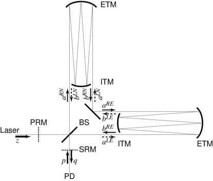
Figure 1: Schematic plot of a Sagnac interferometer with optical delay lines in the arms.

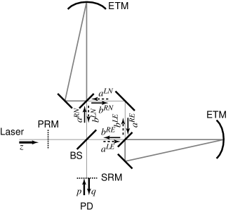
Figure 2: Schematic plot of a Sagnac interferometer with ring cavities in the arms.

II The Sagnac as a speed meter, and its input-output relations

II.1 The Sagnac optical configuration

Two variants of Sagnac interferometers are shown in Figs. 1 and 2, which uses optical delay lines or ring-shaped Fabry-Perot cavities in the arms. [The idea of using optical delay lines and ring cavities are due to Drever, proposed in similar designs. See, e.g., Ref. Drever .] In both variants, the carrier light enters the interferometer from the left port (also called the “bright port”) of the beamsplitter (BS). The light gets split in two and travels into the two arms in opposite orders; we denote by R the beam that enters the North (N) arm first and the East (E) arm second, and by L that which enters E first and N second. Suppose the mirrors are all held fixed at their equilibrium positions, so that the two arms are exactly symmetric; then the carrier R and L beams, upon arriving again at the beamsplitter, will combine in such a way that no lights exits to the port below the beamsplitter (the “dark port”). Similarly, any vacuum fluctuations that enter the interferometer at the bright port along with the carrier light will also be suppressed in the dark-port output. Only vacuum fluctuations that entered the interferometer from the dark port can leave the interferometer through the dark port. As a result, the dark port is decoupled from the bright port, as in a Michelson interferometer. This fact is crucial to the suppression of laser noise in the dark-port output.

II.2 The Sagnac’s Speed-Meter Behavior

When the end mirrors of the two arms are allowed to move, they phase modulate the carrier light, generating sideband fields. Only antisymmetric, non-static changes in the arm lengths can contribute to the dark-port output; this is a result of the cancellation at the beamsplitter, and the fact that the two beams pass through the two arms in the opposite order. A more detailed but still rough exploration of this point reveals the Sagnac’s role as a speed-meter interferometer:

Denoting by $\tau_{\mathrm{arm}}$ the (average) storage time of light in the arms and by $x_{\mathrm{N},\,\mathrm{E}}$ the time-dependent displacements of the end mirrors, we have for the phase gained by the R and L beams after traveling from the bright entry port through the two arms to the dark exit port:

$$\delta\phi_{\mathrm{R}} \sim \mathrm{x}_{\mathrm{N}}(t)+x_{\mathrm{E}}(t+\tau_{\mathrm{arm}})\,,$$

$$\delta\phi_{\mathrm{L}} \sim \mathrm{x}_{\mathrm{E}}(t)+x_{\mathrm{N}}(t+\tau_{\mathrm{arm}})\,.$$

The amplitude of the dark-port output is proportional to the phase difference of the two beams at the beamsplitter:

$$\delta\phi_{\mathrm{R}}-\delta\phi_{\mathrm{L}} \sim \left[x_{\mathrm{N}}(t)-x_{\mathrm{N}}(t+\tau_{\mathrm{arm}})\right]$$ (1)

$$- \left[x_{\mathrm{E}}(t)-x_{\mathrm{E}}(t+\tau_{\mathrm{arm}})\right]\,.$$

As a consequence, the Sagnac interferometer is not sensitive to any time-independent displacement of the test masses. By expanding Eq. (1) in powers of $\tau_{\rm arm}$, we see that, at frequencies much smaller than $1/\tau_{\mathrm{arm}}$, the speed of the test-mass motion is measured, and at higher frequencies, a mixture of the speed and its time derivatives is measured — as also is the case in other speed meters SMorig ; SMP ; SMPC .

II.3 Input-output relations without a signal-recycling mirror

As a foundation for evaluating the performances of Sagnac interferometers in the high-power regime, we shall now derive their quantum mechanical input-output relations — i.e., we shall derive equations for the quantum mechanical dark-port output field $q$ in terms of the input (vacuum) fields $p$ at the dark port and $z$ at the bright port (which in the end does not appear in $q$), and the gravitational-wave field $h$. In Figs. 1 and 2, we have denoted by $a^{\mathrm{RN},\,\mathrm{RE},\,\mathrm{LN},\,\mathrm{LE}}$ the input sideband fields of the R and L beams at the N and E arms, and by $b^{\mathrm{RN},\,\mathrm{RE},\,\mathrm{LN},\,\mathrm{LE}}$ the output sideband fields. For the moment, we shall ignore the existence of the signal-recycling mirror (SRM); and throughout we shall ignore the power-recycling mirror (PRM) since (as for Michelson topologies) it merely serves to provide a larger input power at the beamsplitter and has no other significance for the interferometer’s quantum noise.

In this paper, we shall use the Caves-Schumaker two-photon formalism Caves_Schumaker (briefly introduced in Sec. IIA of KLMTV), which breaks the time-domain sideband fields, at any given spatial location, into the following form,

$$E(t)=\sqrt{\frac{4\pi\hbar\omega_{0}}{{\mathcal{A}}c}}\left[E_{1}(t)\cos(\omega_{0}t)+E_{2}(t)\sin(\omega_{0}t)\right]\,,$$ (2)

where $\omega_{0}$ is the carrier frequency, ${\cal A}$ is the cross sectional area of the beam. Here $E_{1,2}(t)$ are slowly varying fields called the cosine (or amplitude) and sine (or phase) quadratures. These quadratures fields can be thought of as amplitude or phase modulations on a carrier field of the form $D\cos(\omega_{0}t)$ . The quadrature fields can be expanded as

$$E_{1,2}(t)=\int_{0}^{+\infty}\frac{d\Omega}{2\pi}\left(a_{1,2}e^{-i\,\Omega\,t}+a_{1,2}^{\dagger}e^{+i\,\Omega\,t}\right)\,,$$ (3)

in terms of the quadrature operators $a_{1,2}(\Omega)$. A more general quadrature operator can be constructed from $a_{1,2}$:

$$a_{\Phi}=a_{1}\cos\Phi+a_{2}\sin\Phi\,.$$ (4)

The set of propagation equations common to both of our Sagnac configurations [with either delay lines (DL for short) or ring cavities (FP for short) inside the arms] are: (i) at the beamsplitter,

$$a^{\mathrm{RN}}=\frac{z+p}{\sqrt{2}}\,,\quad a^{\mathrm{LE}}=\frac{z-p}{\sqrt{2}}\,,\quad q=\frac{b^{\mathrm{LN}}-b^{\mathrm{RE}}}{\sqrt{2}}\,;$$ (5)

and (ii) when the beams leave one arm and enter the other,

$$a^{\mathrm{RE}}=b^{\mathrm{RN}}\,,\quad a^{\mathrm{LN}}=b^{\mathrm{LE}}\,.$$ (6)

The above equations, (5) and (6), are for both quadratures. By writing down these equations, we assume the distances between the BS and ITMs to be small, and also integer multiples of the laser wavelength.

	DL	FP
$\Psi_{\mathrm{arm}}$	$\displaystyle\mathcal{B}\Omega L/c$	$\displaystyle\arctan\left(\frac{1+\sqrt{R}}{1-\sqrt{R}}\tan\frac{\Omega L}{c}\right)$
$\mathcal{K}_{\mathrm{arm}}$	$\displaystyle\frac{8I_{\mathrm{c}}\omega_{0}}{m\mathcal{B}\Omega^{2}c^{2}}\left(\frac{\sin\mathcal{B}\Omega L/c}{\sin\Omega L/c}\right)^{2}$	$\displaystyle\frac{8I_{\mathrm{c}}\omega_{0}}{m\Omega^{2}c^{2}}\left(\frac{T}{1-2\sqrt{R}\cos(2\Omega L/c)+R}\right)$
$\Psi_{\mathrm{sagnac}}$	$\displaystyle 2\mathcal{B}\Omega L/c+\pi/2$	$\displaystyle 2\arctan\left(\frac{1+\sqrt{R}}{1-\sqrt{R}}\tan\frac{\Omega L}{c}\right)+\pi/2$
$\mathcal{K}_{\mathrm{sagnac}}$	$\displaystyle\frac{32I_{\mathrm{c}}\omega_{0}}{mLc\left(\frac{c}{L\mathcal{B}}\right)^{3}}\left[\frac{\sin^{2}(\mathcal{B}\Omega L/c)}{(\mathcal{B}\Omega L/c)(\mathcal{B}\sin\Omega L/c)}\right]^{2}$	$\displaystyle\frac{32I_{\mathrm{c}}\omega_{0}}{m\Omega^{2}c^{2}}\left[\frac{(1+\sqrt{R})\sqrt{T}\sin(\Omega L/c)}{1-2\sqrt{R}\cos(2\Omega L/c)+R}\right]^{2}$

Table 1: Expressions for $\Psi_{\mathrm{arm}}$, $\mathcal{K}_{\mathrm{arm}}$, $\Psi_{\mathrm{sagnac}}$ and $\mathcal{K}_{\mathrm{sagnac}}$ in the DL and FP cases.

The input-output relations for the arms, i.e., the $b$-$a$ relations, are evaluated in the Appendix (in an manner analogous to that of KLMTV for Michelson configurations), for the distinct cases of DL and FP. The results can be put into the following simple form:

$$b_{1}^{IJ} = e^{2i\Psi_{\mathrm{arm}}}a_{1}^{IJ}\,,$$ (7)

$$b_{2}^{IJ} = e^{2i\Psi_{\mathrm{arm}}}\left[a_{2}^{IJ}-\mathcal{K}_{\mathrm{arm}}(a_{1}^{\mathrm{L}J}+a_{1}^{\mathrm{R}J})\right]$$ (8)

$$+e^{i\Psi_{\mathrm{arm}}}\frac{\sqrt{2\mathcal{K}_{\mathrm{arm}}}}{h_{\mathrm{SQL}}}\sqrt{2}\,\tilde{x}_{J}^{\mathrm{GW}}/L\,.$$

Here $I=\mathrm{L},\,\mathrm{R}$ stands for either one of the two beams, and $J=\mathrm{E},\,\mathrm{N}$ stands for either one of the two arms. The quantity $\tilde{x}_{J}^{\rm GW}$ is the gravitational-wave induced displacement of the $J$th ETM (in frequency domain), $L$ is the arm length, and $m$ is the mass of the ITM and the ETM. The Standard Quantum Limit is given by

$$h_{\mathrm{SQL}}=\sqrt{\frac{8\hbar}{m\Omega^{2}L^{2}}}\,.$$ (9)

Expressions for $\Psi_{\mathrm{arm}}$ and $\mathcal{K}_{\mathrm{arm}}$, in the cases of DL and FP, are given in the Appendix [Eqs. (41), (42), (52) and (53)] and summarized in Table. 1. Combining Eqs. (5)–(8), we obtain $q_{1,2}$ in terms of the input fields and the dimensionless gravitational-wave strain (in frequency domain), $\tilde{h}$ [also using $\tilde{h}=(\tilde{x}_{\mathrm{E}}^{\mathrm{GW}}-\tilde{x}_{\mathrm{N}}^{\mathrm{GW}})/L$]:

$$q_{1} = e^{2i\Psi_{\mathrm{sagnac}}}p_{1}\,,$$ (10)

$$q_{2} = e^{2i\Psi_{\mathrm{sagnac}}}(p_{2}-\mathcal{K}_{\mathrm{sagnac}}p_{1})$$ (11)

$$+ e^{i\Psi_{\mathrm{sagnac}}}\frac{\sqrt{2\mathcal{K}_{\mathrm{sagnac}}}}{h_{\mathrm{SQL}}}\tilde{h}\,;$$

with

$$\Psi_{\mathrm{sagnac}} = 2\Psi_{\mathrm{arm}}+\frac{\pi}{2}\,,$$ (12)

$$\mathcal{K}_{\mathrm{sagnac}} = 4\mathcal{K}_{\mathrm{arm}}\sin^{2}\Psi_{\mathrm{arm}}\,.$$ (13)

Expressions for $\Psi_{\mathrm{sagnac}}$ and $\mathcal{K}_{\mathrm{sagnac}}$ in the DL and FP cases can be obtained by inserting Eqs. (41), (42), (52) and (53) into Eqs. (12) and(13), with results summarized again in Table. 1. Indeed, as mentioned at the beginning of this section, the bright-port input field $z$ does not appear in the dark-port output quadratures, $q_{1,2}$.

The input-output relations (10) and (11) have the same general form as those of a conventional Michelson interferometer, Eq. (16) of KLMTV , and those of a Michelson speed meter, Eqs. (27) of SMP or Eqs. (12) of SMPC . In particular, as discussed in the Appendix, the output phase quadrature $q_{2}$ is a sum of three terms: the shot noise (first term), the radiation-pressure noise (second term) and the gravitational-wave signal (third term), while the output amplitude quadrature $q_{1}$ contains only shot noise.

II.4 Influence of signal recycling on the input-output relations

Since the input-output relations of Sagnac interferometers have the same form as those of a conventional Michelson interferometer, the quantum noise of signal-recycled Sagnac interferometers can be obtained easily using the results of Refs. BC1 ; BC2 . For simplicity, we shall restrict the signal-recycling cavity to be either resonant with the carrier frequency (“tuned SR”) or anti-resonant (“tuned RSE”), leaving the detuned case for future investigations. In these cases, the dynamics of the interferometer are not modified by the signal recycling, and the input-output relation has the same form as Eqs. (10) and (11), with $\mathcal{K}_{\mathrm{sagnac}}$ replaced by (see Sec. IIIC of Ref. BC1 )

$$\mathcal{K}_{\mathrm{sagnac}\,\mathrm{SR}}=\frac{\tau^{2}}{1-2\rho\cos 2\Psi_{\mathrm{sagnac}}+\rho^{2}}\mathcal{K}_{\mathrm{sagnac}}\,,$$ (14)

and $\Psi_{\rm sagnac}$ replaced by a quantity $\Psi_{\rm sagnac\,SR}$ whose value is not of interest to us. Here $\rho$ and $\tau$ are the (amplitude) reflectivity and transmissivity of the signal-recycling mirror, with $\rho\in\Re$, $\tau>0$ and $\rho^{2}+\tau^{2}=1$. The quantity $\phi$ is the detuning of the signal-recycling cavity, related to its length by $l$ (which is defined as the distance from the beamsplitter to the signal-recycling mirror) by $\phi=[\omega_{0}l/c]_{\rm mod\,2\pi}$. It is also assumed that the length $l$ is very short, so $\Omega l/c$ can be regarded as $0$. Expressions for $\mathcal{K}_{\mathrm{sagnac}\,\mathrm{SR}}$ can be obtained by using results in Table 1.

Using the fact that $\Omega L/c\ll 1$ (for earth-based interferometers in the high-frequency band), $\mathcal{B}\gg 1$ (for the DL case) and $T\ll 1$ (for the FP case), we can obtain some approximate formulas for $\mathcal{K}_{\mathrm{sagnac}\,\mathrm{SR}}$ (which also apply to the non-SR case, with $\rho\rightarrow 0$ and $\tau\rightarrow 1$): in the DL case

$$\mathcal{K}_{\mathrm{sagnac}\,\mathrm{SR}}^{\mathrm{DL}}= \frac{32I_{\mathrm{c}}\omega_{0}}{mLc\gamma_{\mathrm{DL}}^{3}}\left[\frac{\tau^{2}}{1+2\rho\cos(4\Omega/\gamma_{\mathrm{DL}})+\rho^{2}}\right]$$ (15)

$$\times\left[\frac{\sin(\Omega/\gamma_{\mathrm{DL}})}{\Omega/\gamma_{\mathrm{DL}}}\right]^{4}\,,$$

with

$$\gamma_{\mathrm{DL}}=\frac{c}{{\mathcal{B}}L}\,;$$ (16)

and in the FP case

$$\mathcal{K}_{\mathrm{sagnac}\,\mathrm{SR}}^{\mathrm{FP}}=\frac{16I_{\mathrm{c}}\omega_{0}}{mLc}\frac{\delta}{(\Omega^{2}-\Omega_{\mathrm{s}}^{2})^{2}+\delta^{2}\Omega^{2}}\,;$$ (17)

with

$$\delta=2\left(1+\frac{T}{2}\right)\frac{1-\rho}{1+\rho}\gamma_{\mathrm{FP}}\,\quad\Omega_{\mathrm{s}}=\left(1+\frac{T}{2}\right)\gamma_{\mathrm{FP}}\,,$$ (18)

where

$$\gamma_{\mathrm{FP}}=\frac{Tc}{4L}\,.$$ (19)

Interestingly, Eq. (17) is identical to Eqs. (22) and (23) of Ref. SMPC , with substitutions (this paper $\rightarrow$ Purdue and Chen) $I_{c}\rightarrow W_{\mathrm{circ}}$ (circulating power), $\Omega_{\mathrm{s}}\rightarrow\Omega$ (sloshing frequency), $\delta\rightarrow\delta$ (extraction rate), $\Omega\rightarrow\omega$ (sideband frequency), and $\mathcal{K}_{\mathrm{sagnac}\,\mathrm{SR}}^{\mathrm{FP}}\rightarrow\kappa$. As we shall explain further in the following sections, the coupling constant $\mathcal{K}_{\rm sagnac\,SR}$ alone (besides $h_{\rm SQL}$, which depends on $m$ and $L$) will determine the quantum noise of the interferometer. This means that a signal-recycled Sagnac interferometer with ring cavities in its arms is equivalent to the Michelson speed meters proposed in Refs. SMP ; SMPC (if we ignore the influence of optical losses and other noise sources).

II.5 Frequency dependence of coupling constants $\mathcal{K}$, and Sagnac interferometers as speed meters

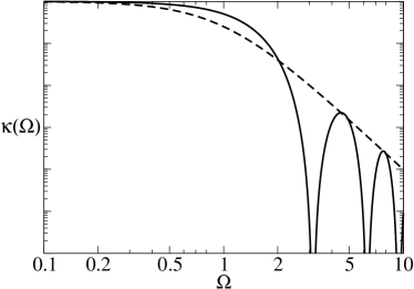
Figure 3: The coupling constant $\mathcal{K}_{\rm sagnac}(\Omega)$ for non-signal-recycled DL [in solid line, Eq. (15) with $\rho=0$, $\tau=1$] and FP [in dashed line, Eq. (17) with $\delta=2\Omega_{\rm s}$] sagnac interferometers, in arbitrary (logarithmic) units, with $\Omega$ measured in units of $\gamma_{\mathrm{DL}}$ (DL case) and $\Omega_{\mathrm{s}}$ (FP case), respectively.

As can be seen both analytically in Eqs. (17) and (18) and graphically in Fig. 3, the coupling constant $\mathcal{K}_{\rm sagnac}$ of a Sagnac interferometer without signal recycling (i.e., $\tau=1$, $\rho=0$) approaches a constant as $\Omega\rightarrow 0$, which also turns out to be its maximum. This fact, combined with the input-output relation (11), suggests that the second output quadrature $q_{2}$ is indeed sensitive to the speed of the interferometer induced by the gravitational wave, since at low frequencies

$$q_{2}(\mathrm{signal}\,\mathrm{part})\propto\Omega\sqrt{\mathcal{K}(\Omega=0)}\tilde{x}^{\mathrm{GW}}\propto\mathrm{momentum}\,.$$ (20)

(A more detailed discussion of the link between $\mathcal{K}$ and a speed meter’s performance is given in Sec. IIIA of Ref. SMPC ; that discussion, in the framework of a Michelson speed meter, is equally valid for a Sagnac speed meter.) When signal recycling is added, the shape of $\mathcal{K}(\Omega)$ can be adjusted for optimization purposes; examples are shown in Fig. 4.

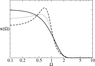
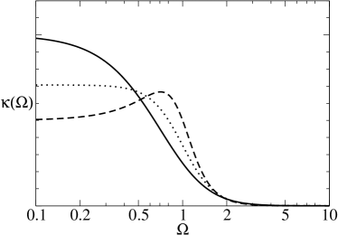
Figure 4: The coupling constant $\mathcal{K}_{\rm sagnac\,SR}(\Omega)$ for signal-recycled DL [left panel, Eq. (15)] and FP [right panel, Eq. (17)] Sagnac interferometers, in arbitrary (linear) units, with $\Omega$ measured in units of $\gamma_{\mathrm{DL}}$ (DL case) and $\Omega_{\mathrm{s}}$ (FP case), respectively. For DL: cases with $\rho=0$ (solid curve), 0.1 (dotted curve) and 0.2 (dashed curve) are plotted . For FP cases with $\delta=2\Omega_{\mathrm{s}}$ (solid curve), $\sqrt{2}\Omega_{\mathrm{s}}$ (dotted curve), and $\Omega_{\mathrm{s}}$ (dashed curve) are plotted, corresponding to $\rho=0$, 0.172, and 0.333.

III Noise spectral density

In this section, we shall assume that homodyne detection can be carried out on any (frequency-independent) quadrature,

$$q_{\Phi}=q_{1}\cos\Phi+q_{2}\sin\Phi\,.$$ (21)

Homodyne detection is essential for QND interferometers, if they are to beat the SQL by substantial amounts; the additional noise associated with heterodyne detection schemes can seriously limit an interferometer’s ability to beat the SQL rfmod .

The noise spectral density associated with the input-output relations (10) and (11) can be obtained in a manner analogous to that of Sec. IV of KLMTV or Sec. III of Ref. SMPC . The result is

$$S_{h}=\left[\frac{(\cot\Phi-\mathcal{K}_{\mathrm{sagnac}\,\mathrm{SR}})^{2}+1}{2\mathcal{K}_{\mathrm{sagnac}\,\mathrm{SR}}}\right]h_{\mathrm{SQL}}^{2}\,.$$ (22)

As is also discussed in Refs. SMBGKT ; SMP ; SMPC , the optimal quadrature to observe is the one with

$$\cot\Phi=\mathcal{K}_{\mathrm{max}}\equiv\max_{\Omega}\mathcal{K}_{\mathrm{sagnac}\,\mathrm{SR}}(\Omega)\,;$$ (23)

for this quadrature the noise spectral density is

$$S_{h}=\left[\frac{(\mathcal{K}_{\mathrm{max}}-\mathcal{K}_{\mathrm{sagnac}\,\mathrm{SR}})^{2}+1}{2\mathcal{K}_{\mathrm{sagnac}\,\mathrm{SR}}}\right]h_{\mathrm{SQL}}^{2}\,.$$ (24)

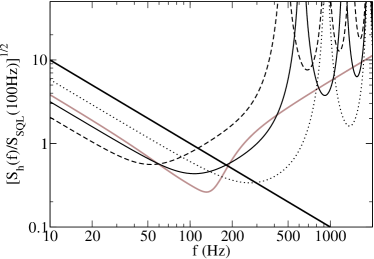
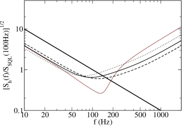
Figure 5: The noise spectral density [for the optimized quadrature, see Eq. (23)] of non-signal-recycled DL (left panel) and FP (right panel) Sagnac interferometers [Eq. (24), setting $\rho=1$ and $\tau=0$], assuming $I_{\mathrm{c}}=8.2\,\mathrm{MW}$ and $m=40\,\mathrm{kg}$. [By injecting squeezed vacuum (with squeeze factor $e^{-2R}$) into the dark port, one can reduce $I_{\mathrm{c}}$ by a factor $e^{2R}\sim 10$.] For DL: cases with $\mathcal{B}=40$ (dotted curve), 60 (solid curve) and 80 (dashed curve) are plotted. For FP: cases with $\Omega_{\mathrm{s}}=2\pi\times 200\,\mathrm{Hz}$ (dotted curve), $2\pi\times 220\,\mathrm{Hz}$ (solid curve) and $2\pi\times 240\,\mathrm{Hz}$ (dashed curve) are plotted. The noise curves for the fiducial speed meter (in gray) and the SQL (dark straight lines) are also plotted in both panels for comparison.

In the left panel of Fig. 5, we plot the noise spectral density of a delay-line Sagnac interferometer without signal recycling, with $m=40\,\mathrm{kg}$ and $I_{\mathrm{c}}=8.2\,\mathrm{MW}$ (the characteristic circulating power used for the Michelson speed meter in Refs. SMP ; SMPC ), and with $\mathcal{B}=$40, 60, 80 [corresponding to powers in a single beam equal to $102.5\,\mathrm{kW}$, $68.3\,\mathrm{kW}$ and $51.3\,\mathrm{kW}$, respectively; see Eq. (33); these powers can be lowered by injecting squeezed vacuum into the dark port, as we shall discuss below]. The noise spectral density of the fiducial Michelson speed meter of Refs. SMP ; SMPC , with the same $I_{\mathrm{c}}$ and $m$, and (in their notation) $\Omega=2\pi\times 173\,\mathrm{Hz}$, $\delta=2\pi\times 200\,\mathrm{Hz}$, is also plotted for comparison. In the right panel, we plot the noise spectral density of a ring-cavity Sagnac interferometer without signal recycling, with the same $m$ and $I_{\mathrm{c}}$, and with $\gamma_{\mathrm{FP}}=2\pi\times 200\,\mathrm{Hz}$, $2\pi\times 220\,\mathrm{Hz}$ and $2\pi\times 240\,\mathrm{Hz}$. As one can see in the two panels, both configurations of non-recycled Sagnac interferometers exhibit broadband QND performance, with the beating of the SQL concentrated at low frequencies.

Signal recycling allows us to improve and optimize the Sagnac interferometers so they have similar performance to a Michelson speed meter; i.e., so they beat the SQL by a roughly constant factor over a substantially broader frequency band than without signal recycling. In particular, since the spectral density (22) only depends on $\mathcal{K}$, and $\mathcal{K}_{\mathrm{sagnac}\,\mathrm{SR}}^{\mathrm{FP}}$ is the same as that of a Michelson speed meter, the signal-recycled Sagnac interferometers with ring cavities will have the same performance as the Michelson speed meters. In Fig. 6, we give one example for each of the DL and FP configurations. In the left panel we plot the noise spectral density for a signal-recycled DL Sagnac with $m=40\,\mathrm{kg}$, $I_{\mathrm{c}}=8.2\,\mathrm{MW}$, $\mathcal{B}=60$ (and therefore $I_{\mathrm{b}}=68\,\mathrm{kW}$) and $\rho=0.09$ (dark solid curve), compared with that of the corresponding non-recycled ($\rho=0$) interferometer (dashed curve), and that of the fiducial Michelson speed meter (gray solid curve). In the right panel we plot the the noise spectral density of a signal-recycled FP Sagnac interferometer with $T=0.0564$, $\rho=0.268$, corresponding to $\Omega_{\mathrm{s}}=2\pi\times 173\,\mathrm{Hz}$, and $\delta=2\pi\times 200\,\mathrm{Hz}$ [from Eq. (18)]. This interferometer has the same noise spectral density as the fiducial Michelson speed meter. [The two noise curves agree perfectly, appearing as the solid curve in the panel.] The corresponding non-recycled noise curve (with $\rho=0$) is also plotted (the dashed curve) for comparison.

As conceived by Caves Caves and discussed in Refs. KLMTV ; SMPC , injecting squeezed vacuum into the dark-port can lower the required circulating power. For example, as discussed in Sec. IVA of Ref. SMPC , for speed meters with input-output relations with the form of Eqs. (10) and (11), the circulating power can be lowered by the squeeze factor $e^{-2R}$, while maintaining the same performance. In the LIGO-III era, it is reasonable to expect $e^{-2R}\sim 0.1$ KLMTV , so the circulating powers cited above can be lowered by a factor $\sim 10$. The resulting fiducial circulating power, $I_{c}=8.2\mathrm{MW}/10=820\mathrm{kW}$ is about the same as planned for the second-generation Advanced LIGO interferometers.

Finally, for signal-recycled FP Sagnac interferometers, since they are equivalent to the Michelson speed meters of Ref. SMPC , one can further improve the high-frequency performance by performing frequency-dependent homodyne detection with the aid of two kilometer-scale optical filters at the dark-port output; see Sec. IVB of SMPC .

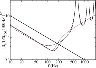
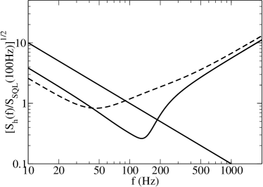
Figure 6: The solid curves are the noise spectral densities of signal-recycled DL (left panel) and FP (right panel) Sagnac interferometers [Eq. (24)], assuming $I_{\mathrm{c}}=8.2\,\mathrm{MW}$ and $m=40\,\mathrm{kg}$. [By injecting squeezed vacuum into the dark port, one can reduce $I_{\mathrm{c}}$ by a factor $e^{2R}\sim 10$.] For DL, we take $\mathcal{B}=60$, $\rho=0.09$; for FP, we take $\Omega_{\mathrm{s}}=2\pi\times 173\,\mathrm{Hz}$ and $\delta=2\pi\times 200\,\mathrm{Hz}$, which correspond to $T=0.0564$ and $\rho=0.268$. The corresponding non-recycled noise curves are also shown, as dashed curves. The noise curve of the fiducial Michelson speed meter is plotted in gray in the left panel and is identical to the solid, signal-recycled FP Sagnac noise curve in the right panel; the standard quantum limit is shown as dark straight lines.

IV Discussion of technical issues

We shall now comment on three technical issues that might affect significantly the performances of Sagnac speed-meter interferometers:

Optical Losses. So far in this paper, we have regarded all interferometers as ideal; most importantly, we have ignored optical losses. As has been shown by several studies of the Michelson case KLMTV ; SMPC , optical losses can sometimes be the limiting factor on the sensitivity of a QND interferometer. However, as shown in Ref. SMPC , Michelson speed meters are less susceptible to optical losses than Michelson position meters (even though the losses may be enhanced by the larger number of optical surfaces on which to scatter or absorb, and by the fact that the coupling constant $\mathcal{K}(\Omega)$ remains finite as $\Omega\rightarrow 0$ rather than growing to infinity). It is plausible that this feature will be retained, at least for optical losses associated with the individual optical elements, and with the readout scheme, but rigorous calculations are yet to be carried out. Moreover, the losses due to the use of diffractive optics and polarization techniques in some Sagnac configurations AllReflective deserve serious study.

High Power Through the Beam Splitter. As we saw at the end of Sec. III, for FP Sagnac interferometers, in order to optimize the shape of the noise curve, the required values of the power transmissivity of the ITM can become as large as $0.05$, which may require optical powers at the level of tens of kilowatts through the beamsplitter (even when squeezed vacuum is injected into the dark port); this may pose a problem for implementation. In Michelson speed meters, a resonant-side-band-extraction technique can be used to greatly reduce the power through the beamsplitter without affecting the interferometer’s performance, but it is not clear whether an analogous trick exists for Sagnac interferometers.

Susceptibility to Mirror Tilt and Imperfections. In the low-laser-power limit, the Sagnac interferometer is known to be more susceptible to mirror tilting than are Michelson interferometers, but less susceptible to geometric imperfections of mirrors PGM98 . A study of these susceptibilities needs to be carried out in the context of high laser power, in order to see whether they pose any serious difficulty in the implementation of Sagnac speed meters.

V Conclusions

In this paper, a quantum-mechanical study of idealized Sagnac interferometers, including radiation-pressure effects, has been carried out. As was already known, Sagnac interferometers are sensitive only to the time varying part of the antisymmetric mode of mirror displacement. It was a short and trivial step, in this paper, to demonstrate that this means a Sagnac interferometer measures the test masses’ relative speed or momentum and therefore is a speed meter with QND capabilities. Detailed computations revealed that, as for other speed meters, a broad-band QND performance can be obtained, when frequency-independent homodyne detection is performed at the dark port. Signal recycling can be employed to further optimize the noise spectrum so it is comparable to that of a Michelson speed meter (or exactly the same, for Sagnac configurations with ring cavities in the arms); and, by contrast with the Michelson, this can be achieved without the need for any additional kilometer-scale FP cavity. [In the case of frequency-dependent homodyne detection with the aid of two kilometer-scale filter cavities, the Sagnac speed meter still needs one less optical cavity than its Michelson counterpart.] If further technical issues, including those related to optical losses (Sec. IV), can be resolved, the Sagnac optical topology will be a strong candidate for third-generation gravitational-wave interferometers, such as LIGO-III and EURO.

Appendix A Input-output relations for the arms

Since the north and east arms are identical, we need only analyze one of them. For concreteness, we study the East arm. In Appendix B of Ref. KLMTV , KLMTV derived the input-output relation for a simple FP cavity, using the same Caves-Schumaker quadrature formalism Caves_Schumaker as we use here. The input-output relations for optical delay-line arms and ring cavities can be derived analogously:

A.1 Optical delay line

Following the procedure of KLMTV, we initially suppose that the ITM is not moving, and we denote the displacement of the ETM by $x_{\mathrm{E}}(t)$. Suppose the R beam has an electric field amplitude

$$E^{\mathrm{RE}\,\mathrm{in}}(t)=[D+E^{\mathrm{RE}\,\mathrm{in}}_{1}(t)]\cos\omega_{0}t+E^{\mathrm{RE}\,\mathrm{in}}_{2}(t)\sin\omega_{0}t$$ (25)

at the location where it enters the E arm; here $D$ is the (classical) carrier amplitude and $E^{\mathrm{RE}\,\mathrm{in}}_{1,2}(t)$ are the sideband quadrature fields

$$E^{\mathrm{RE}\,\mathrm{in}}_{1,2}(t)=\sqrt{\frac{4\pi\hbar\omega_{0}}{{\mathcal{A}}c}}\int_{0}^{+\infty}\frac{d\Omega}{2\pi}\left[a^{\mathrm{RE}}_{1,2}e^{-i\,\Omega\,t}+h.c.\right]\,,$$ (26)

with “h.c.” meaning “Hermitian conjugate”. The output beam after $\mathcal{B}$ bounces is delayed by

$$\Delta t=2\mathcal{B}L/c+2\big{[}x_{\mathrm{E}}(t-L/c)+x_{\mathrm{E}}(t-3L/c)+\cdots+x_{\mathrm{E}}(t-(2\mathcal{B}-1)L/c)\big{]}\,,$$ (27)

so

$$E^{\mathrm{RE}\,\mathrm{out}}(t)=E^{\mathrm{RE}\,\mathrm{in}}(t-\Delta t) \approx [D+E^{\mathrm{RE}\,\mathrm{in}}_{1}(t-2\mathcal{B}L/c)]\cos\omega_{0}t+E^{\mathrm{RE}\,\mathrm{in}}_{2}(t-2\mathcal{B}L/c)\sin\omega_{0}t$$ (28)

$$+ \frac{2\omega_{0}D}{c}\sum_{k=1}^{\mathcal{B}}x_{\mathrm{E}}\left(t-(2k-1)L/c\right)\,.$$

Comparing with

$$E^{\mathrm{RE}\,\mathrm{out}}_{1,2}(t)=\sqrt{\frac{4\pi\hbar\omega_{0}}{{\mathcal{A}}c}}\int_{0}^{+\infty}\frac{d\Omega}{2\pi}\left[b^{\mathrm{RE}}_{1,2}e^{-i\,\Omega\,t}+h.c.\right]\,,$$ (29)

we obtain

$$b^{\mathrm{RE}}_{1} = e^{2i\mathcal{B}\Omega L/c}a_{1}^{\mathrm{RE}}\,,$$ (30)

$$b_{2}^{\mathrm{RE}} = e^{2i\mathcal{B}\Omega L/c}a_{2}^{\mathrm{RE}}+\frac{2\omega_{0}}{c}\sqrt{\frac{2I_{\mathrm{b}}}{\hbar\omega_{0}}}\left(\frac{\sin\mathcal{B}\Omega L/c}{\sin\Omega L/c}\right)e^{i\mathcal{B}\Omega L/c}\tilde{x}_{\mathrm{E}}\,.$$ (31)

where $\tilde{x}_{\mathrm{E}}$ is the Fourier transform of $x_{\mathrm{E}}(t)$. Here $I_{\mathrm{b}}$ is the power of the beam,

$$I_{\mathrm{b}}=\frac{D^{2}{\mathcal{A}}c}{8\pi}\,,$$ (32)

which is related to the total circulating power by

$$I_{\mathrm{b}}=\frac{I_{\mathrm{c}}}{2\mathcal{B}}\,.$$ (33)

The physical meanings of Eqs. (30) and (31) can be roughly explained as follows: (i) the gravitational-wave signal embodied in $\tilde{x}_{\mathrm{E}}$ is only present in the second (phase) quadrature, $b^{\mathrm{RE}}_{2}$, of the output sideband field, i.e., in the second term of the right-hand side of Eq. (31); (ii) the first term on the right-hand sides of Eqs. (30) and (31) represents the shot noise, which originates from the quantum fluctuations of the input field. Obviously, the relations (30) and (31) also apply to the L beam, with the change of superscript R to L.

Next we must study the motion of the end mirror, which is influenced by both the passing gravitational wave and the radiation-pressure force:

$$x_{\mathrm{E}}=x^{\mathrm{GW}}_{\mathrm{E}}+x_{\mathrm{E}}^{\mathrm{BA}}\,,\quad\ddot{x}_{\mathrm{BA}}=\frac{1}{m}F_{\mathrm{RP}}.$$ (34)

Here $x_{\mathrm{BA}}$ is the displacement induced by the radiation-pressure force, or the back action of the measurement process, which eventually gives rise to the radiation-pressure noise. The radiation-pressure force $F_{\mathrm{RP}}$ comes from both the L and R beams:

$$F_{\mathrm{RP}}(t)=\frac{{\mathcal{A}}}{2\pi}\sum_{k=1}^{\mathcal{B}}\left\{\left[E^{\mathrm{RE}\,\mathrm{in}}(t-(2k-1)L/c)\right]^{2}+\left[E^{\mathrm{LE}\,\mathrm{in}}(t-(2k-1)L/c)\right]^{2}\right\}\,.$$ (35)

However, we are only interested in the fluctuating and low-frequency part (in the gravitational-wave band) of the force, which comes from the beating of the sideband fields against the carrier:

$$F^{\mathrm{fluc}}_{\mathrm{RP}}(t)=\frac{D{\mathcal{A}}}{2\pi}\sum_{k=1}^{\mathcal{B}}\left[E_{1}^{\mathrm{RE}\,\mathrm{in}}(t-(2k-1)L/c)+E_{1}^{\mathrm{LE}\,\mathrm{in}}(t-(2k-1)L/c)\right]\,.$$ (36)

Combining Eqs. (34) and (36) and transforming into the frequency domain, we obtain the Fourier transform of the mirror displacement in the GW frequency band [note that Eq. (32) is used again]:

$$\tilde{x}_{\mathrm{E}}=\tilde{x}_{\mathrm{E}}^{\mathrm{GW}}-\frac{4}{m\Omega^{2}c}\sqrt{2\hbar\omega_{0}I_{\mathrm{b}}}\left(\frac{\sin\mathcal{B}\Omega L/c}{\sin\Omega L/c}\right)e^{i\mathcal{B}\Omega L/c}\left(\frac{a^{\mathrm{RE}}_{1}+a^{\mathrm{LE}}_{1}}{2}\right)\,.$$ (37)

This, when combined with Eq. (31), yields:

$$b_{2}^{\mathrm{RE}}=e^{2iB\Omega L/c}a_{2}^{\mathrm{RE}}-\frac{16I_{\mathrm{b}}\omega_{0}}{m\Omega^{2}c^{2}}\left(\frac{\sin\mathcal{B}\Omega L/c}{\sin\Omega L/c}\right)^{2}e^{2i\mathcal{B}\Omega L/c}\left(\frac{a_{1}^{\mathrm{RE}}+a_{1}^{\mathrm{LE}}}{2}\right)+\frac{2\omega_{0}}{c}\sqrt{\frac{2I_{\mathrm{b}}}{\hbar\omega_{0}}}\left(\frac{\sin\mathcal{B}\Omega L/c}{\sin\Omega L/c}\right)\tilde{x}_{\mathrm{E}}^{\mathrm{GW}}\,.$$ (38)

The second term on the right-hand side is the radiation-pressure noise. In reality, the internal mirrors (ITM’s), the beamsplitter, and the connection mirror will also move under the radiation-pressure force (but they are not influenced by gravitational waves). When $\mathcal{B}\gg 1$ and $\Omega L/c\ll 1$, only the internal mirrors need be taken into account, and the effect is just a doubling of the radiation pressure noise in Eq. (38). Hence we arrive at the complete input-output relation for the East arm, put into a more compact form (similar to those in KLMTV KLMTV ):

$$b^{\mathrm{RE}}_{1} = e^{2i\Psi_{\mathrm{DL}}}a^{\mathrm{RE}}_{1}\,,$$ (39)

$$b_{2}^{\mathrm{RE}} = e^{2i\Psi_{\mathrm{DL}}}\left[a_{2}^{\mathrm{RE}}-\mathcal{K}_{\mathrm{DL}}(a_{1}^{\mathrm{RE}}+a^{\mathrm{LE}}_{1})\right]+e^{i\Psi_{\mathrm{DL}}}\frac{\sqrt{2\mathcal{K}_{\mathrm{DL}}}}{h_{\mathrm{SQL}}}\sqrt{2}\,\tilde{x}^{\mathrm{GW}}_{E}/L\,;$$ (40)

where

$$\Psi_{\mathrm{DL}} = \mathcal{B}\Omega L/c\,,$$ (41)

$$\mathcal{K}_{\mathrm{DL}} = \frac{16I_{\mathrm{b}}\omega_{0}}{m\Omega^{2}c^{2}}\left(\frac{\sin\mathcal{B}\Omega L/c}{\sin\Omega L/c}\right)^{2}=\frac{8I_{\mathrm{c}}\omega_{0}}{m\mathcal{B}\Omega^{2}c^{2}}\left(\frac{\sin\mathcal{B}\Omega L/c}{\sin\Omega L/c}\right)^{2}\,.$$ (42)

The input-output relation for the L beam can be obtained by exchanging RE and LE in Eqs. (39) and (40).

A.2 Ring cavity

Again, let us consider the East arm. Suppose again, for the moment, that only the ETM is allowed to move. Then the input-output relations for the fields immediately inside the ITM can be obtained easily from the results for optical delay lines [Eqs. (39)–(42), with a factor $1/2$ multiplying the radiation-pressure noise term, since again as a first step we are only allowing the ETM to move]:

$$B_{1}^{\mathrm{RE}} = e^{2i\Omega L/c}A_{1}^{\mathrm{RE}}\,,$$ (43)

$$B_{2}^{\mathrm{RE}} = e^{2i\Omega L/c}\left[A_{2}^{\mathrm{RE}}-\mathcal{K}^{\mathcal{B}=1}_{\mathrm{DL}}\left(\frac{A_{1}^{\mathrm{RE}}+A_{1}^{\mathrm{LE}}}{2}\right)\right]+e^{i\Omega L/c}\frac{\sqrt{2\mathcal{K}_{\mathrm{DL}}^{\mathcal{B}=1}}}{h_{\mathrm{SQL}}}\sqrt{2}\,\tilde{x}_{\mathrm{E}}/L\,;$$ (44)

where

$$\mathcal{K}_{\mathrm{DL}}^{B=1}=\frac{8I_{\mathrm{c}}\omega_{0}}{m\Omega^{2}c^{2}}\,.$$ (45)

As before, the input-output relation for the L beam is obtained by exchanging RE and LE. The fields outside the ITM are related to these fields by

$$b^{\mathrm{RE}}_{1,2}=-\sqrt{R}a_{1,2}^{\mathrm{RE}}+\sqrt{T}B^{\mathrm{RE}}_{1,2}\,,\quad\quad A^{\mathrm{RE}}_{1,2}=\sqrt{T}a_{1,2}^{\mathrm{RE}}+\sqrt{R}B^{\mathrm{RE}}_{1,2}\,;$$ (46)

$$b^{\mathrm{LE}}_{1,2}=-\sqrt{R}a_{1,2}^{\mathrm{LE}}+\sqrt{T}B^{\mathrm{LE}}_{1,2}\,,\quad\quad A^{\mathrm{LE}}_{1,2}=\sqrt{T}a_{1,2}^{\mathrm{LE}}+\sqrt{R}B^{\mathrm{LE}}_{1,2}\,.$$ (47)

Combining Eqs. (43)–(47), we obtain

$$b_{1}^{\mathrm{RE}} =\frac{e^{2i\Omega L/c}-\sqrt{R}}{1-e^{2i\Omega L/c}\sqrt{R}}a_{1}^{\mathrm{RE}}\,,$$ (48)

$$b_{2}^{\mathrm{RE}} =\frac{e^{2i\Omega L/c}-\sqrt{R}}{1-e^{2i\Omega L/c}\sqrt{R}}\left[a_{2}^{\mathrm{RE}}-\frac{T\mathcal{K}_{\mathrm{DL}}^{\mathcal{B}=1}}{1-2\sqrt{R}\cos(2\Omega L/c)+R}\left(\frac{a_{1}^{\mathrm{RE}}+a_{1}^{\mathrm{LE}}}{2}\right)\right]$$ (49)

$$+\frac{e^{i\Omega L/c}\sqrt{T}}{1-e^{2i\Omega L/c}\sqrt{R}}\frac{\sqrt{2\mathcal{K}_{\mathrm{DL}}^{\mathcal{B}=1}}}{h_{\mathrm{SQL}}}\sqrt{2}\,\tilde{x}_{\mathrm{E}}/L\,.$$

As before, the first terms on the right-hand sides of Eqs. (50) and (51) represent the shot noise, the second term on the right-hand side of Eq. (51) represents the radiation-pressure noise, and the third term on the right-hand side of Eq. (51) is the gravitational-wave signal. Again, other optical elements besides the ETM can also be influenced by the radiation-pressure force; but when $T\ll 1$, we need only consider the radiation-pressure force on the ITM and the other cavity mirror near the ITM. Suppose all three sides of the ring cavity are on resonance with the carrier frequency. Then it is obvious that, at leading order in $\Omega L/c$ and $T$, the fluctuating forces associated with the beams at the locations of the three mirrors are the same. However, since the in-cavity light is incident on the two near mirrors at $45^{\circ}$, the motions of each of them induced by the radiation pressure is $1/\sqrt{2}$ that of the ITM, in the direction normal to their surfaces. Also because their motion directions are again $45^{\circ}$ to the propagation direction of the beams, the resulting radiation-pressure noise is reduced by an additional $1/\sqrt{2}$. In the end, the net radiation-pressure noise due to the two near mirrors is equal to that due to the end mirror. Doubling the radiation-pressure noise in Eq. (51), we obtain the input-output relation of the ring cavity, which we put into a form similar to that of the optical delay line:

$$b^{\mathrm{RE}}_{1} = e^{2i\Psi_{\mathrm{FP}}}a^{\mathrm{RE}}_{1}\,,$$ (50)

$$b_{2}^{\mathrm{RE}} = e^{2i\Psi_{\mathrm{FP}}}\left[a_{2}^{\mathrm{RE}}-\mathcal{K}_{\mathrm{FP}}(a_{1}^{\mathrm{RE}}+a^{\mathrm{LE}}_{1})\right]+e^{i\Psi_{\mathrm{FP}}}\frac{\sqrt{2\mathcal{K}_{\mathrm{FP}}}}{h_{\mathrm{SQL}}}\sqrt{2}\,\tilde{x}^{\mathrm{GW}}_{E}/L\,;$$ (51)

with

$$\Psi_{\mathrm{FP}} = \arg\frac{e^{i\Omega L/c}}{1-e^{2i\Omega L/c}\sqrt{R}}=\arctan\left(\frac{1+\sqrt{R}}{1-\sqrt{R}}\tan\frac{\Omega L}{c}\right)\,,$$ (52)

$$\mathcal{K}_{\mathrm{FP}} = \left(\frac{T}{1-2\sqrt{R}\cos 2\Omega L/c+R}\right)\frac{8I_{\mathrm{c}}\omega_{0}}{m\Omega^{2}c^{2}}\,.$$ (53)

References

- (1) V. B. Braginsky and F. Ya. Khalili, Phys. Lett. A 147, 251 (1990).
- (2) V. B. Braginsky, M. L. Gorodetsky, F. Ya. Khalili, and K. S. Thorne, Phys. Rev. D 61, 044002 (2000).
- (3) P. M. Purdue, Phys. Rev. D 66, 022001 (2002).
- (4) P. Purdue and Y. Chen, submitted to Phys. Rev. D.
- (5) A. Abramovici et al., Science 256, 325 (1992); B. Caron et al., Class. Quantum Grav. 14, 1461 (1997); H. Lück et al., Class. Quantum Grav. 14, 1471 (1997); M. Ando et al., Phys. Rev. Lett. 86, 3950 (2001).
- (6) K. S. Thorne, “The scientific case for mature LIGO interferometers,” LIGO Document Number P000024-00-R, www.ligo.caltech.edu/docs/P/P000024-00.pdf; C. Cutler and K. S. Thorne, “An overview of gravitational-wave sources,” gr-qc/0204090.
- (7) E. Gustafson, D. Shoemaker, K.A. Strain and R. Weiss, “LSC White paper on detector research and development,” LIGO Document Number T990080-00-D, www.ligo.caltech.edu/docs/T/T990080-00.pdf.
- (8) LCGT Collaboration, Int. J. of Mod. Phys. D, Vol. 8, 557 (1999).
- (9) G. Sagnac, C. R. Acad. Sci. 95, 1410 (1913).
- (10) R. W. P. Drever, in Gravitational Radiation, edited by N. Deruelle and T. Piran (North-Holland, Amsterdam, 1983).
- (11) K.-X. Sun, M. M. Fejer, E. Gustafson and R. L. Byer, Phys. Rev. Lett, 76, 3053 (1996); The TAMA team, Gravitational-wave Astronomy, Report for the Japanese government, Kyoto University, pp 286–287 (1992); R. Weiss, in NSF proposal, 1987.
- (12) D. A. Shaddock, M. B. Gray and D. E. McClelland, Appl. Opt. 37, 7995 (1998).
- (13) B. Petrovichev, M. Gray and D. McClelland, Gen. Rel. and Grav., 30, 1055 (1998).
- (14) J. Mizuno, A. Rüdiger, R. Schilling, W. Winkler and K. Danzmann, Opt. Comm. 138, 383 (1997)
- (15) K.-X. Sun and R. L. Byer, Gen. Rel. and Grav., 23, 567 (1998); S. Traeger, P. Beyersdorf, L. Goddard, E. K. Gustafson, M. M. Fejer and R. L. Byer, Opt. Lett., 25, 722 (2000); P. Beyersdorf, The Polarization Sagnac interferometer for gravitational-wave detection, Ph.D. Thesis, Stanford University, Feb. 2001.
- (16) Although there are not yet detailed papers on EURO or LIGO-III, they have been discussed within the gravitational-wave community as long-range plans.
- (17) V. B. Braginsky, Sov. Phys. JETP 26, 831 (1968); V. B. Braginsky and Yu. I. Vorontsov, Sov. Phys. Usp. 17, 644 (1975); V.B. Braginsky, Yu. I. Vorontsov, and F. Ya. Khalili, Sov. Phys. JETP, 46, 705 (1977).
- (18) V. B. Braginsky and F.Ya. Khalili, Quantum measurement, edited by K. S. Thorne (Cambridge University Press, Cambridge, England, 1992).
- (19) A. Buonanno and Y. Chen, Class. Quantum Grav. 18, L95 (2001).
- (20) A. Buonanno and Y. Chen, Phys. Rev. D 64, 042006 (2001).
- (21) A. Buonanno and Y. Chen, Phys. Rev. D 65, 042001 (2002); Class. Quantum Grav. 19 1569 (2002).
- (22) B. J. Meers, Phys. Rev. D 38, 2317 (1988); J. Y. Vinet, B. Meers, C. N. Man and A. Brillet, Phys. Rev. D 38, 433 (1988).
- (23) J. Mizuno, Comparison of optical configurations for laser-interferometric gravitational-wave detectors, PhD thesis, Max-Planck Institut f’́ur Quantenoptik, Garching, Germany, 1995; J. Mizuno, K. A. Strain, P. G. Nelson, J. M. Chen, R. Schilling, A. Rüdiger, W. Winkler and K. Danzmann, Phys. Lett. A 175, 273 (1993) .
- (24) S.P. Vyatchanin and A.B. Matsko, JETP 77, 218 (1993); S.P. Vyatchanin and E.A. Zubova, Phys. Lett. A 203, 269 (1995); S.P. Vyatchanin and A.B. Matsko, JETP 82, 1007 (1996); ibid. JETP 83, 690 (1996) ; S.P. Vyatchanin, Phys. Lett. A 239, 201 (1998).
- (25) H. J. Kimble, Yu. Levin, A. B. Matsko, K.S. Thorne and S. P. Vyatchanin, Phys. Rev. D 65, 022002 (2002).
- (26) W.G. Unruh, Phys. Rev. D 19, 2888 (1979); C. M. Caves, K. S. Thorne, R. W. P. Drever, V. D. Sandberg, and M. Zimmerman, Rev. of Mod. Phys., 52, 341 (1980); C. M. Caves, in Quantum Optics, Experimental Gravity and Measurement Theory, edited by P. Meystre and M. O. Scully (Plenum, New York, 1982), p. 567.
- (27) C. M. Caves and B. L. Schumaker, Phys. Rev. A 31 3068 (1985); B. L. Schumaker and C.M. Caves, Phys. Rev. A 31 3093 (1985).
- (28) T. M. Niebauer, R. Schilling, K. Danzmann, A. Rüdiger, W. Winkler, Phys. Rev. A 43, 5022 (1991); B. J. Meers and K. A. Strain, Phys. Rev. A 44, 4693 (1991); A. Buonanno, Y. Chen and N. Mavalvala, in preparation.
- (29) C. M. Caves, in Quantum Optics, Experimental Gravitation, and Measurement Theory, edited by P. Meystre and M. O. Scully (Plenum, New York, 1982), p. 567.