Spatially Averaged Quantum Inequalities Do Not Exist in Four-Dimensional Spacetime

Abstract

We construct a particular class of quantum states for a massless, minimally coupled free scalar field which are of the form of a superposition of the vacuum and multi-mode two-particle states. These states can exhibit local negative energy densities. Furthermore, they can produce an arbitrarily large amount of negative energy in a given region of space at a fixed time. This class of states thus provides an explicit counterexample to the existence of a spatially averaged quantum inequality in four-dimensional spacetime.

I Introduction

It is well known that quantum fields can produce local renormalized negative energy densities. This is despite the fact that the classical expression for the energy density appears to be positive definite. The negative energy density is possible because renormalization involves an infinite subtraction, and is needed to make the stress tensor operator well-defined. If there were no restrictions on the sorts of negative energy densities attainable, one could have a number of bizarre possibilities, including traversable wormholes MT ; MTY , faster-than-light travel A ; K ; Olum time travel MT ; MTY ; E , and violations of the second law of thermodynamics F78 . Such phenomena are, at best, rare.

Fortunately, there are known to be severe constraints on the magnitude and duration of negative energy fluxes or densities, at least in the case of linear fields. These are the quantum inequalities, which take the typical form F91 ; FR95 ; FR97 ; FLAN ; PF971 ; PFGQI ; FE

$$\int_{-\infty}^{\infty}\langle:T_{00}({\bf x},t):\rangle\,F(t)\,dt\geq-\frac{c}{t_{0}^{d}}\,.$$ (1)

Here $\langle:T_{00}({\bf x},t):\rangle$ is the renormalized energy density in an arbitrary quantum state, $F(t)$ is a normalized sampling function with a characteristic width $t_{0}$, $c$ is a dimensionless constant, usually somewhat less than unity, and $d$ is the dimension of spacetime. Most of the work on quantum inequalities is for the cases of $d=2$ and $d=4$. More precisely, Eq. (1) is a worldline quantum inequality for an inertial observer in Minkowski spacetime, where $t$ is the observer’s proper time. (Recently, worldline inequalities have been established in much greater generality in globally hyperbolic spacetimes Fewster .) The physical interpretation of this constraint is that there is an inverse relation between the magnitude of the negative energy and its duration. For example, in four dimensions, the observer will not see the negative energy last for a time longer than about $|\rho_{max}|^{-\frac{1}{4}}$, where $\rho_{max}$ is the maximally negative energy density seen by this observer. This type of constraint greatly limits the macroscopic effects of negative energy. In particular, macroscopic wormholes or “warp drive” spacetimes are severely constrained FRWH ; PFWD ; ER . Furthermore, one can use the worldline inequalities to place some constraints on the spatial distribution of negative energy BFR02 . All allowed spatial distributions must be such that Eq. (1) is satisfied for every inertial observer in Minkowski spacetime.

There is a different type of constraint on the energy density, which is that the total energy in any quantum state for a quantum field in boundary-free Minkowski spacetime must be non-negative. Let the Hamiltonian operator be

$$H=\int d^{d-1}x\,:T_{00}({\bf x},t):\,,$$ (2)

where the integral is taken over all space at a fixed time. The expectation value of $H$ in an arbitrary quantum state is non-negative:

$$\langle H\rangle\geq 0\,,$$ (3)

and $\langle H\rangle=0$ only in the vacuum state. Thus any non-vacuum state must have net positive energy, even though there can be local regions with negative energy density.

This raises the question of whether there are spatial or spacetime quantum inequalities analogous to Eq. (1), but involving sampling over space or space and time. For spacetime averages, there is an abstract existence proof for a very general class of such inequalities in globally hyperbolic spacetimes. These include, for example, inequalities bounding violations of the dominant energy condition Helfer99 . However, at present quantitative estimates for these are not known.

One can get some spacetime quantum inequalities by simply averaging the worldline inequalities over families of worldlines with spatial weighting factors, but in at least some cases these are known not to be sharp. For example, stronger constraints were found in two-dimensional Minkowksi space FLAN ; Roman97 . We may express these as

$$\int dx\,dt\,F_{S}(x)\,F_{T}(t)\,\langle:T_{00}({x},t):\rangle\,\geq-B(x_{0},t_{0})\,.$$ (4)

Here $F_{S}(x)$ is a spatial sampling function with width $x_{0}$, $F_{T}(t)$ is a temporal sampling function with width $t_{0}$, and the bound $B(x_{0},t_{0})$ is finite as long as at least one of $x_{0}$ and $t_{0}$ is nonzero. The sampling functions are assumed to be each normalized to unity:

$$\int dx\,F_{S}(x)\;=\;\int dt\,F_{T}(t)\;=\,1\,.$$ (5)

If the sampling functions are both Lorentzian functions, then $B\propto(x_{0}+t_{0})^{-2}$; if they are both Gaussians, then $B\propto(x_{0}^{2}+t_{0}^{2})^{-1}$. In either case, one obtains the corresponding worldline inequality when $x_{0}=0$, and a nontrivial bound on the spatially sampled energy density when $t_{0}=0$. One consequence of this is that in two dimensions the spacetime averaged results are stronger than the temporally averaged ones, since as $t_{0}\to 0$ (for $x_{0}>0$) one gets a finite bound.

It is natural to ask if there is a generalization of Eq. (4) to four-dimensional spacetime, especially one which gives a nontrivial bound when the sampling is over space only. One of us Helfer96 has given an argument that this is not the case, and that the spatially sampled energy density can be unbounded below. Actually, the argument was written out there for a more generic situation, that of evolution from a Cauchy surface in a general curved spacetime. While explicit constructions were given in this case, they were by pseudodifferential operator techniques, and they were not translated into more conventional quantum field-theoretic terms. Also, the details of the more special case of a surface of constant time in Minkowski space were not written out. So no explicit version of the argument in conventional special-relativistic quantum field-theoretic terms has yet been given. The purpose of the present paper is to provide such an example and to draw as many physical insights as possible from it. In the following section, we will provide the explicit construction of a class of quantum states for the massless, minimally coupled scalar field, with negative energy density, as well as give the two-point function and the energy density in this class of states. We then show that although this state satisfies Eq. (1), the spatially sampled energy density can be arbitrarily negative. Further implications of this example are discussed in Sect. III. We work in units where $\hbar=c=1$. (A related construction has subsequently been used, in Ref. FewR , to prove that there are no quantum inequalities along null geodesics in four-dimensional Minkowski spacetime.)

II The Energy Density in a Class of Quantum States

II.1 Characterization of the State

The particular quantum states which will be used in this paper are of the form of a superposition of the vacuum and a multi-mode two-particle state:

$$|\psi\rangle=N\left[|0\rangle+\sum_{{\bf k}_{1},{\bf k}_{2}}c_{{\bf k}_{1},{\bf k}_{2}}\,|{{\bf k}_{1},{\bf k}_{2}}\rangle\right]\,,$$ (6)

where we assume that the $c_{{\bf k}_{1},{\bf k}_{2}}$’s are symmetric. Here $|{{\bf k}_{1},{\bf k}_{2}}\rangle$ is a two-particle state containing a pair of particles with momenta ${\bf k}_{1}$ and ${\bf k}_{2}$, and the normalization factor is

$$N=\left[1+\xi\sum_{{\bf k}_{1},{\bf k}_{2}}|c_{{\bf k}_{1},{\bf k}_{2}}|^{2}\right]^{-\frac{1}{2}}\,,$$ (7)

where $\xi=2$ if ${\bf k}_{1}\not={\bf k}_{2}$ and $\xi=1$ if ${\bf k}_{1}={\bf k}_{2}$. Note that each of the two-particle states in Eq. (6) appears twice, since $|{{\bf k}_{1},{\bf k}_{2}}\rangle=|{{\bf k}_{2},{\bf k}_{1}}\rangle$; this leads to the factor of $2$ in Eq. (7) when ${\bf k}_{1}\not={\bf k}_{2}$. We can quantize the scalar field in a box of volume $V$, so that the momenta are discrete. Later, we will let $V\rightarrow\infty$, so that

$$\sum_{\bf k}\rightarrow\frac{V}{(2\pi)^{3}}\,\int d^{3}k\,.$$ (8)

In this limit, we replace the coefficients $c_{{\bf k}_{1},{\bf k}_{2}}$ by functions of continuous momenta defined by

$$b({\bf k}_{1},{\bf k}_{2})=\frac{V}{(2\pi)^{3}}\,c_{{\bf k}_{1},{\bf k}_{2}}\,.$$ (9)

The normalization factor then becomes

$$N=\left[1+2\int d^{3}k_{1}\,d^{3}k_{2}\,|b({\bf k}_{1},{\bf k}_{2})|^{2}\right]^{-\frac{1}{2}}\,.$$ (10)

The quantum state is also characterized by a cutoff $\Lambda$, so that $|{\bf k}_{1}|,|{\bf k}_{2}|<\Lambda$. Later, we will consider the limit in which the cutoff is removed, $\Lambda\rightarrow\infty$. We will require that the functional form of $b({\bf k}_{1},{\bf k}_{2})$ be such that the integral in Eq. (5) remain finite in this limit.

The particular choice of $b({\bf k}_{1},{\bf k}_{2})$ which we adopt is the following:

$$b({\bf k}_{1},{\bf k}_{2})=\chi({\bf k}_{1}+{\bf k}_{2})\,(|{\bf k}_{1}||{\bf k}_{2}|)^{\nu-\frac{1}{2}}\,,$$ (11)

where

$$\chi({\bf p})=\left\{\begin{array}[]{ll}\chi_{0}\,,&\mbox{if $|{\bf p}|\leq p_{0}$}\\ 0\,,&\mbox{otherwise}\end{array}\right.$$ (12)

where $\chi_{0}$ and $p_{0}$ are arbitrary constants. (The function $\chi({\bf p})$ is taken to have a sharp cutoff merely for convenience; it could be made smooth without affecting our essential argument.) Thus our state is really a four-parameter family of states defined by the parameters $\Lambda$, $\nu$, $\chi_{0}$, and $p_{0}$. We will be especially interested in the limit in which the magnitudes of the momenta of both particles become large with $p_{0}$ fixed. In this limit, the pairs of particles have almost exactly opposite momenta.

The integral in Eq. (5) can now be written as

$$\chi_{0}^{2}\,\int d^{3}k\,\int_{|{\bf p}|\leq p_{0}}d^{3}p\,(|{\bf k}||{\bf k-p}|)^{2\nu-1}\,,$$ (13)

where ${\bf k}={\bf k}_{1}$ and ${\bf p}={\bf k}_{1}+{\bf k}_{2}$. In the limit that $\Lambda\rightarrow\infty$, the $k$-integration will converge at the upper limit provided that

$$\nu<-\frac{1}{4}\,.$$ (14)

This is the condition that our quantum state be normalizable in the $\Lambda\rightarrow\infty$ limit.

II.2 The Two-Point Function

Now we wish to calculate the form of the two-point function for the massless scalar field in the states we have selected. First expand the field operator in terms of mode functions and creation and annihilation operators as

$$\varphi=\sum_{\bf k}(a_{\bf k}f_{\bf k}+a^{\dagger}_{\bf k}f^{*}_{\bf k})$$ (15)

where the mode functions are

$$f_{\bf k}=\frac{1}{\sqrt{2\omega V}}\,{\rm e}^{i({\bf k}\cdot{\bf x}-\omega\,t)}\,,$$ (16)

with $\omega=|{\bf k}|$.

We are interested in the renormalized two-point function in the state $|\psi\rangle$, defined by

$$\langle:\varphi(x)\,\varphi(x^{\prime}):\rangle=\langle\psi|\varphi(x)\,\varphi(x^{\prime})|\psi\rangle-\langle 0|\varphi(x)\,\varphi(x^{\prime})|0\rangle\,.$$ (17)

It may be expressed as

$$\langle:\varphi(x)\,\varphi(x^{\prime}):\rangle = \sum_{{\bf k},{\bf k^{\prime}}}\Bigl{[}f^{*}_{\bf k}(x)f_{\bf k^{\prime}}(x^{\prime})\,\langle a^{\dagger}_{\bf k}a_{\bf k^{\prime}}\rangle+f_{\bf k}(x)f^{*}_{\bf k^{\prime}}(x^{\prime})\,\langle a^{\dagger}_{\bf k^{\prime}}a_{\bf k}\rangle$$ (18)

$$+ f_{\bf k}(x)f_{\bf k^{\prime}}(x^{\prime})\,\langle a_{\bf k}a_{\bf k^{\prime}}\rangle+f^{*}_{\bf k}(x)f^{*}_{\bf k^{\prime}}(x^{\prime})\,\langle a^{\dagger}_{\bf k}a^{\dagger}_{\bf k^{\prime}}\rangle\Bigr{]}\,,$$

where the expectation values are in the state $|\psi\rangle$.

If we evaluate this expression explicitly using the form of the quantum state in Eq. (6) and of the mode functions in Eq. (16), and then take the infinite volume limit, using Eq. (9), the result is

$$\langle:\varphi(x)\,\varphi(x^{\prime}):\rangle=\frac{2N^{2}}{(2\pi)^{3}}\,{\rm Re}\int d^{3}k\,d^{3}k^{\prime}\,\frac{1}{\sqrt{\omega\omega^{\prime}}}\,$$ (19)

$$\times \Bigl{[}2{\rm e}^{i({\bf k^{\prime}}\cdot{\bf x^{\prime}}-{\bf k}\cdot{\bf x})}{\rm e}^{i(\omega\,t-\omega^{\prime}\,t^{\prime})}\,\int d^{3}k_{1}b^{*}({\bf k}_{1},{\bf k})b({\bf k}_{1},{\bf k^{\prime}})$$

$$+ {\rm e}^{i({\bf k}\cdot{\bf x}+{\bf k^{\prime}}\cdot{\bf x^{\prime}})}{\rm e}^{-i(\omega\,t+\omega^{\prime}\,t^{\prime})}\,b({\bf k},{\bf k^{\prime}})\Bigr{]}\,.$$

The first term on the righthand side, which is quadratic in $b$, comes from the expectation value in the two-particle component of $|\psi\rangle$ alone, whereas the second term, which is linear in $b$, comes from a cross term involving both the vacuum and the two-particle component. It is the latter part which will be of greater interest to us. So long as $\Lambda<\infty$, the integrals in Eq. (19) exist and define smooth functions of $x$ and $x^{\prime}$, so the two-point function has the Hadamard form. More precisely, the behavior as $x\to x^{\prime}$ has the Hadamard form. The falloff as the separation between $x$ and $x^{\prime}$ increases will be slow, on account of the sharp cutoff in $\chi(p)$. Had we used a modified $\chi$, falling off smoothly, we could have arranged for a more rapid falloff as the spatial separation of $x$ and $x^{\prime}$ becomes large.

II.3 The Energy Density

The energy density in a given quantum state may be obtained from the renormalized two-point function. For the massless, minimally coupled scalar field, we can write

$$\rho=\frac{1}{2}\lim_{{{\bf x^{\prime}}\rightarrow{\bf x}}\atop{t^{\prime}\rightarrow t}}\left[(\partial_{t}\partial_{t^{\prime}}+\mbox{\boldmath$\nabla\cdot\nabla^{\prime}$})\,\langle:\varphi(x)\,\varphi(x^{\prime}):\rangle\right]\,.$$ (20)

We may now use Eq. (19) to write the energy density as

$$\rho = \frac{N^{2}}{(2\pi)^{3}}\,{\rm Re}\int d^{3}k\,d^{3}k^{\prime}\,\sqrt{\omega\omega^{\prime}}\,(1+\hat{{\bf k}}\cdot\hat{{\bf k}}^{\prime})\,\Bigl{[}2{\rm e}^{i({\bf k^{\prime}}-{\bf k})\cdot{\bf x}}{\rm e}^{i(\omega-\omega^{\prime})t}\,\int d^{3}k_{1}b^{*}({\bf k}_{1},{\bf k})b({\bf k}_{1},{\bf k^{\prime}})$$ (21)

$$- {\rm e}^{i({\bf k}+{\bf k^{\prime}})\cdot{\bf x}}{\rm e}^{-i(\omega+\omega^{\prime})t}\,b({\bf k},{\bf k^{\prime}})\Bigr{]}\,,$$

where $\hat{{\bf k}}$ and $\hat{{\bf k}}^{\prime}$ are unit vectors in the directions of ${\bf k}$ and ${\bf k^{\prime}}$, respectively. Let $\rho_{1}$ denote the term quadratic in $b$, and $\rho_{2}$ denote the term linear in $b$.

Let us first examine the behavior of $\rho_{2}$. If we use the explicit form for $b$ given in Eq. (11), and let ${\bf p}={\bf k}+{\bf k^{\prime}}$, we find

$$\rho_{2}=-\frac{\chi_{0}N^{2}}{(2\pi)^{3}}\,{\rm Re}\int d^{3}k\,\int_{|{\bf p}|\leq p_{0}}d^{3}p\,\sqrt{\omega\omega^{\prime}}\,(1+\hat{{\bf k}}\cdot\hat{{\bf k}}^{\prime})\,{\rm e}^{i{\bf p}\cdot{\bf x}}\,{\rm e}^{-i(\omega+|{\bf p}-{\bf k}|)t}\,(\omega|{\bf p}-{\bf k}|)^{\nu-\frac{1}{2}}\,.$$ (22)

In the limit that $\omega$ becomes large compared to $p_{0}$, we can expand the product $\hat{{\bf k}}\cdot\hat{{\bf k}}^{\prime}$ as follows:

$$\hat{{\bf k}}\cdot\hat{{\bf k}}^{\prime} = \frac{\hat{{\bf k}}\cdot({\bf p}-{\bf k})}{\sqrt{({\bf p}-{\bf k})\cdot({\bf p}-{\bf k})}}=\left(-1+\frac{\hat{{\bf k}}\cdot{\bf p}}{\omega}\right)\left[1-2\frac{\hat{{\bf k}}\cdot{\bf p}}{\omega}+\frac{p^{2}}{\omega^{2}}\right]^{-\frac{1}{2}}$$ (23)

$$\approx -1+\frac{p^{2}-(\hat{{\bf k}}\cdot{\bf p})^{2}}{2\omega^{2}}+\cdots\,.$$

To leading order when $\omega\gg p_{0}$, we can write $\omega^{\prime}\approx\omega$. If the integral for $\rho_{2}$ is dominated by values of $\omega$ large compared to $p_{0}$, we have

$$\rho_{2}\approx-\frac{\chi_{0}N^{2}}{2(2\pi)^{3}}\,{\rm Re}\int d^{3}k\,\int_{|{\bf p}|\leq p_{0}}d^{3}p\,\,\omega^{2(\nu-1)}\,[p^{2}-(\hat{{\bf k}}\cdot{\bf p})^{2}]\,{\rm e}^{i{\bf p}\cdot{\bf x}}\,{\rm e}^{-2i\omega t}\,.$$ (24)

We next perform the angular integrations. If we integrate over the directions of ${\bf k}$ with ${\bf p}$ fixed, we find

$$\int d^{3}k\,p^{2}=4\pi p^{2}\int d\omega\,\omega^{2}$$ (25)

and

$$\int d^{3}k\,(\hat{{\bf k}}\cdot{\bf p})^{2}=2\pi p^{2}\int d\omega\,\omega^{2}\,\int_{-1}^{1}dc\,c^{2}=\frac{4\pi}{3}p^{2}\int d\omega\,\omega^{2}\,,$$ (26)

where $c=\cos\theta$ and $\theta$ is the angle between ${\bf k}$ and ${\bf p}$. Next we integrate over the directions of ${\bf p}$ with ${\bf x}$ fixed to find

$$f_{2}(p_{0},r) \equiv \int_{|{\bf p}|\leq p_{0}}d^{3}p\,p^{2}\,{\rm e}^{i{\bf p}\cdot{\bf x}}=2\pi\int_{0}^{p_{0}}dp\,p^{4}\int_{-1}^{1}dc^{\prime}\,{\rm e}^{iprc^{\prime}}=\frac{4\pi}{r}\int_{0}^{p_{0}}dp\,p^{3}\,\sin(pr)$$ (27)

$$= \frac{4\pi}{r^{5}}\,[3(p_{0}^{2}r^{2}-2)\sin(p_{0}r)-p_{0}r(p_{0}^{2}r^{2}-6)\cos(p_{0}r)]\,,$$

where $r=|{\bf x}|$, $c^{\prime}=\cos\alpha$, and $\alpha$ is the angle between ${\bf x}$ and ${\bf p}$. The function $f_{2}(p_{0},r)$ has the following behavior:

$$f_{2}(p_{0},r)\sim\left\{\begin{array}[]{ll}-(4\pi/r^{2})\,{p_{0}}^{3}\,{\rm cos}\,p_{0}r\,,&\mbox{$r\gg{p_{0}}^{-1}$}\\ (4\pi/5)\,p_{0}^{5}\,,&\mbox{$r\ll{p_{0}}^{-1}$}\end{array}\right.\,.$$ (28)

Now we can write Eq. (24) as

$$\rho_{2}\approx-\frac{\chi_{0}N^{2}}{6\pi^{2}}\,f_{2}(p_{0},r)\,\int_{q_{2}p_{0}}^{\Lambda}d\omega\,\omega^{2\nu}\,\cos(2\omega t)\,,$$ (29)

where $q_{2}$ is a constant chosen so that the approximations made in finding the integrand ($\omega\gg p_{0}$) are valid throughout the range of integration. Note that if $t=0$ and $\nu\geq-\frac{1}{2}$, the integral will diverge in the $\Lambda\rightarrow\infty$ limit.

Let us now set $t=0$ and $\nu=-1/2$. Then the $\omega$-integral becomes

$$\int_{q_{2}p_{0}}^{\Lambda}\frac{d\omega}{\omega}=\ln\left(\frac{\Lambda}{q_{2}p_{0}}\right)\,,$$ (30)

so that

$$\rho_{2}\approx-\frac{\chi_{0}N^{2}}{6\pi^{2}}\,f_{2}(p_{0},r)\,\ln\left(\frac{\Lambda}{q_{2}p_{0}}\right)\,.$$ (31)

We now examine the contribution of $\rho_{1}$. From Eq. (21), we have

$$\rho_{1}=\frac{N^{2}}{(2\pi)^{3}}\,{\rm Re}\int d^{3}k\,d^{3}k^{\prime}\,\sqrt{\omega\omega^{\prime}}\,(1+\hat{{\bf k}}\cdot\hat{{\bf k}}^{\prime})\,\Bigl{[}2{\rm e}^{i({\bf k^{\prime}}-{\bf k})\cdot{\bf x}}{\rm e}^{i(\omega-\omega^{\prime})t}\,\int d^{3}k_{1}b^{*}({\bf k}_{1},{\bf k})b({\bf k}_{1},{\bf k^{\prime}})\Bigr{]}\,.$$ (32)

If we use Eqs. (11) and  (12), letting ${\bf p}={\bf k}_{1}+{\bf k}$ and ${\bf p}^{\prime}={\bf k}_{1}+{\bf k}^{\prime}$, and interchanging the order of integration, we can write

$$\rho_{1} = \frac{2\,{\chi_{0}}^{2}\,N^{2}}{(2\pi)^{3}}\,{\rm Re}\int d^{3}k_{1}\,{|k_{1}|}^{2\nu-1}\,\int_{|{\bf p}|\leq p_{0}}d^{3}p\,\int_{|{\bf p}^{\prime}|\leq p_{0}}d^{3}p^{\prime}\,(1+\hat{{\bf k}}\cdot\hat{{\bf k}}^{\prime})\,$$ (33)

$$\times {(|{\bf p}-{\bf k}_{1}|)}^{\nu}\,{|{\bf p}^{\prime}-{\bf k}_{1}|)}^{\nu}\,{\rm e}^{-i({\bf p}-{\bf p}^{\prime})\cdot{\bf x}}\,{\rm e}^{i[(|{\bf p}-{\bf k}_{1}|)t-(|{\bf p}^{\prime}-{\bf k}_{1}|)t]}\,.$$

If the ${\bf k}_{1}$-integral is dominated by values of $|{\bf k}_{1}|\gg p_{0}$, then we can use ${|{\bf p}-{\bf k}_{1}|}^{\nu}\,\approx{|{\bf p}^{\prime}-{\bf k}_{1}|}^{\nu}\approx{|{\bf k}_{1}|}^{\nu}$. Therefore, at $t=0$ we have

$$\rho_{1}\approx\frac{2\,{\chi_{0}}^{2}\,N^{2}}{(2\pi)^{3}}\,{\rm Re}\int d^{3}k_{1}\,{|k_{1}|}^{4\nu-1}\,\int_{|{\bf p}|\leq p_{0}}d^{3}p\,\int_{|{\bf p}^{\prime}|\leq p_{0}}d^{3}p^{\prime}\,\,(1+\hat{{\bf k}}\cdot\hat{{\bf k}}^{\prime})\,{\rm e}^{-i({\bf p}-{\bf p}^{\prime})\cdot{\bf x}}\,.$$ (34)

Note that in the high $k_{1}$ limit,

$$\hat{{\bf k}}\cdot\hat{{\bf k}}^{\prime}=\frac{({\bf p}-{\bf k}_{1})\cdot({\bf p}^{\prime}-{\bf k}_{1})}{\sqrt{({\bf p}-{\bf k}_{1})\cdot({\bf p}-{\bf k}_{1})}\,\sqrt{({\bf p}^{\prime}-{\bf k}_{1})\cdot({\bf p}^{\prime}-{\bf k}_{1})}}\,\,\rightarrow\,1\,.$$ (35)

As before, we now set $\nu=-1/2$. A similar calculation to that given previously for $\rho_{2}$ yields

$$\rho_{1}\approx\frac{2\,{\chi_{0}}^{2}N^{2}}{\pi^{2}}\,f_{1}(p_{0},r)\,\ln\left(\frac{\Lambda}{q_{1}p_{0}}\right)\,,$$ (36)

where $q_{1}$ is a constant defined analogously to $q_{2}$, and

$$f_{1}(p_{0},r)\equiv\frac{{(4\pi)}^{2}}{r^{6}}\,{[\sin(p_{0}r)-p_{0}r\,\cos(p_{0}r)]}^{2}\,,$$ (37)

and

$$f_{1}(p_{0},r)\sim\left\{\begin{array}[]{ll}{(4\pi p_{0})}^{2}/r^{4}\,{\rm cos}^{2}\,(p_{0}r)\,,&\mbox{$r\gg{p_{0}}^{-1}$}\\ {(4\pi/3)}^{2}\,p_{0}^{6}\,,&\mbox{$r\ll{p_{0}}^{-1}$}\end{array}\right.\,.$$ (38)

Both $|\rho_{2}|$ and $\rho_{1}$ diverge logarithmically, but we can arrange for $|\rho_{2}|/\rho_{1}>1$, provided that

$$\chi_{0}<\frac{1}{12}\,\left(\frac{f_{2}}{f_{1}}\right)\,Y\,,$$ (39)

where

$$Y\equiv\,\left[\frac{\ln\left(\Lambda/q_{2}p_{0}\right)}{\ln\left(\Lambda/q_{1}p_{0}\right)}\right]\rightarrow\,1\,,\,\,\,\,\,\,\,\,\,\mbox{\rm as \,\,\,\,\, $\Lambda\rightarrow\infty$}\,.$$ (40)

This is possible because $\rho_{1}$ and $\rho_{2}$ involve different powers of $\chi_{0}$, stemming from the fact that while $\rho_{1}$ is quadratic in $b$, $\rho_{2}$ is only linear in $b$. (We note in passing that the choice of $\nu=-1/2$ gives $\chi_{0}$ dimensions of length.)

For any value of $p_{0}$, the energy density is approximately constant in space over a region of size, $r\ll{p_{0}}^{-1}$. In this region, $(f_{2}/f_{1})\approx 9/(20\,\pi\,p_{0})$. Choose

$$\chi_{0}<\frac{1}{12}\,\left(\frac{f_{2}}{f_{1}}\right)\,Y\,\approx\frac{3}{80\,\pi\,p_{0}}\,.$$ (41)

where we have used the fact that $Y\rightarrow\,1$, as $\Lambda\rightarrow\infty$. This allows $\rho_{2}$ to dominate $\rho_{1}$, so that $\rho=\rho_{1}+\rho_{2}$ can be made arbitrarily negative over an arbitrarily large region. In summary, we have a normalizable state in which the local energy density may be made arbitrarily negative at time $t=0$ in a finite region of space. It should be pointed out that in the strict $\Lambda\rightarrow\infty$ limit, our state will no longer have the Hadamard form. However, the key point here is that we can consider a sequence of states, each with a finite value of $\Lambda$. Therefore each state in this sequence will have the Hadamard form. By progressively increasing the values of $\Lambda$ as we vary over the states in the sequence, we can make the energy density in our spatially sampled region as negative as we like. In the next section, we will discuss some of the insights which may be drawn from this example.

III Implications and Discussion

We are now in a position to draw a number of conclusions from our example. The first conclusion is the proof that there are no lower bounds on the spatially sampled energy density for the massless minimally coupled scalar field in four spacetime dimensions. To be more precise, consider the spatial average of the energy density

$$S(F)=\int d^{3}x\,F({\bf x})\,\langle:T_{00}({\bf x},t):\rangle$$ (42)

at time $t$, where $F({\bf x})$ is a spatial sampling function. Let $r_{0}$ be the characteristic width of this function. More generally, $r_{0}$ can be the maximum width of $F({\bf x})$ in any direction. If there were to be spatial quantum inequalities here, $S(F)$ would have to have a lower bound when we vary over all quantum states for a given $F({\bf x})$. However, the energy density in the above example varies in space only over a scale of the order of

$$\lambda_{0}=\frac{2\pi}{p_{0}}\,,$$ (43)

which can be arbitrary. Furthermore, we can make the energy density in a region whose size is less than $\lambda_{0}$ arbitrarily negative. For a given sampling function $F({\bf x})$, we can choose $\lambda_{0}>r_{0}$, so that the energy density is approximately constant over the region being sampled and the spatial sampling has no effect, yet the energy density in that region is arbitrarily negative. Thus $S(F)$ is unbounded below. However, this state satisfies the temporal quantum inequality, Eq. (1). One can argue from energy conservation that physically what is happening is that there must be large fluxes of positive energy entering the region, which damp out the negative energy sufficiently for the temporal inequality to hold. Recall from Eqs. (22) and  (33) that $\rho_{2}$ oscillates much more rapidly in time than does $\rho_{1}$. Thus if $\rho_{2}<0$ at one time, it has changed sign a short time later. This causes the time integral of $\rho_{2}$ to tend to average to zero, and allows the worldline quantum inequalities to be satisfied.

We can gain more physical insight into the behavior of this class of states by recalling that in the high frequency limit, the pairs of particles in the two-particle component of the state have nearly but not exactly opposite momenta, as shown in Fig. 1. This allows the scale for the spatial variation of $\rho$ to be large compared to the temporal scale, which is set by the characteristic frequency of the excited modes. This can be seen in Eq. (24), where the spatial factor ${\rm e}^{i{\bf p}\cdot{\bf x}}$ oscillates much more slowly than the temporal factor ${\rm e}^{-2i\omega t}$. One can summarize the difference between the spatial and temporal behaviors by noting that it is possible for the three-momenta of a pair of particles to cancel, but not their energies. We can also see that it is a very special property of two-dimensional spacetime which allows for the existence of spatial bounds. Here the momenta of a pair of particles must be either exactly parallel or exactly anti-parallel. However, if they are anti-parallel, there is a factor analogous to the factor of $1+\hat{{\bf k}}\cdot\hat{{\bf k}}^{\prime}$ in Eq. (21) which suppresses their contribution. Although in this paper we have looked only at four-dimensional spacetime, it seems likely that one can construct similar counterexamples to spatial quantum inequalities in all spacetime dimensions greater than two.

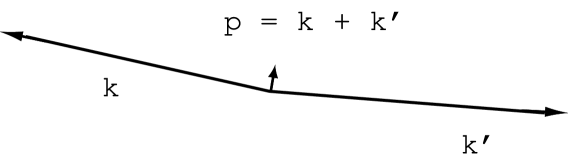
Figure 1: The pairs of particles in the two-particle component of the state have nearly but not exactly opposite momenta, in the high frequency limit. Although their momenta nearly cancel, their energies do not.

We can also understand why the Hamiltonian, obtained by integrating over all space, is bounded below, yet the spatial average over any sampling function with finite width is not. The integration over all space removes the contribution of the $\rho_{2}$ term, leaving only the non-negative contribution of the $\rho_{1}$ term. Thus the net energy in any state must be non-negative. However, it is possible for the spatial distribution at a fixed time to be such that the compensating positive energy is arbitrarily far from the negative energy, and hence violates a spatial quantum inequality.

The current results also shed light on an earlier proposed explanation of the “Garfinkle box”, given in Ref. BFR02 . This refers to an unpublished result of Garfinkle GAR , who showed that the total energy of a scalar field, $E$, contained within an imaginary box in Minkowski spacetime, at fixed time, is unbounded below. The box is “imaginary” in the sense that there are no physical boundaries at the walls of the box. The Garfinkle result is that there exist quantum states for which $E$ is arbitrarily negative. The proposed explanation given in Ref. BFR02 for the unboundedness of the total energy $E$ in this box involved two factors: (1) The energy is measured at a precise instant in time, and (2) the walls of the box are sharply defined. It was argued that this allows an arbitrary amount of negative energy to have entered the box by time $t$, while at this time excluding an even larger amount of positive energy which may be just outside of the box at time $t$. The results of the present paper show that, although this is an explanation of the Garfinkle result, it is not the only explanation. In particular, the unboundedness of the energy in our case does not require the spatial region over which we average to be sharply defined.

In this connection, we emphasize that our results show that the unboundedly negative energies cannot be ascribed to “edge effects” associated with the sampling function. This is because in our examples, the energy density is uniformly negative throughout the sampling region.

While spatially averaged quantum inequalities do not exist, we noted earlier that spacetime averaged ones do. This means that the lower bounds associated with the spacetime averages must diverge as the temporal averaging scale goes to zero. It is natural to conjecture that this is related to the divergence in the spatially averaged inequalities, as follows. Suppose the most severe divergence attainable in the spatial average is

$$\int dx\,F_{S}({\bf x})\,\langle:T_{00}({\bf x},t):\rangle\qquad\hbox{diverges as}\quad-f(\Lambda)\quad\hbox{as}\quad\Lambda\to\infty\,,$$ (44)

for some function $f$ of the ultraviolet cutoff $\Lambda$. Similarly, suppose that for a temporal averaging function $F_{T}(t)$ with characteristic width $t_{0}$, we have

$$\int dx\,dt\,F_{S}({\bf x})\,F_{T}(t)\,\langle:T_{00}({\bf x},t):\rangle\qquad\hbox{diverges as}\quad-g(t_{0})\quad\hbox{as}\quad t_{0}\to 0\,,$$ (45)

for some function $g(t_{0})$. It is natural to ask if $f(\Lambda)\sim g(1/\Lambda)$. A relation like this would probably give the most direct physical significance to the divergences in the spatial averages. (Such a relation would not hold in two dimensions, but might in four.)

The logarithmic divergences (of the energy density with the cutoff $\Lambda$) are rather slow. We do not know whether it is possible to construct examples in Minkowski space with more severe divergences. (In Ref. Helfer96 , more severe divergences were found at Cauchy surfaces with non-zero second fundamental forms. In generic curved spacetimes, this would be the case for all Cauchy surfaces.)

In summary, we have shown that there are no purely spatially averaged quantum inequalities over bounded regions in four-dimensional Minkowski spacetime, even though the integral over all space is bounded. However, spacetime averaged quantum inequalities do exist. As noted earlier, in at least the two-dimensional case, spacetime averaging seems to lead to tighter bounds than does temporal averaging alone. Recent numerical results of Dawson and Fewster DF indicate that similar behavior occurs in four dimensions. However, at present the extent to which spacetime averaging improves temporal averaging is unclear. Thus there appear to be two approaches for better understanding the allowed spatial distributions of negative energy. One is the search for spacetime averaged quantum inequalities, and the other is the continuation of the program begun in Ref. BFR02 , which seeks to extract as much information as possible from the worldline inequalities. Both of these approaches are currently under investigation.

Acknowledgments

The authors would like to thank Chris Fewster for extensive discussions on these issues, and Bill Unruh for useful comments. TAR is grateful to the Tufts Institute of Cosmology, to Werner Israel and the Physics and Astronomy Department of the University of Victoria, and to the Mathematical Physics group at the University of York for their hospitality during this work. LHF and TAR would also like to thank the Erwin Schrödinger Institute in Vienna for hospitality while this work was completed. This research was supported in part by NSF Grants No. Phy-9800965 (to LHF) and No. Phy-9988464 (to TAR).

References

- (1) M.S. Morris and K. Thorne, Am. J. Phys. 56, 395 (1988).
- (2) M.S. Morris, K. Thorne, and U. Yurtsever, Phys. Rev. Lett. 61, 1446 (1988).
- (3) M. Alcubierre, Class. Quantum Grav. 11, L73 (1994).
- (4) S.V. Krasnikov, Phys. Rev. D 57, 4760 (1998), gr-qc/9511068.
- (5) A.E. Everett, Phys. Rev. D 53, 7365 (1996).
- (6) K.D. Olum, Phys. Rev. Lett. 81, 3567 (1998), gr-qc/9806091.
- (7) L.H. Ford, Proc. Roy. Soc. Lond. A 364, 227 (1978).
- (8) L.H. Ford, Phys. Rev. D 43, 3972 (1991).
- (9) L.H. Ford and T.A. Roman, Phys. Rev. D 51, 4277 (1995), gr-qc/9410043.
- (10) L.H. Ford and T.A. Roman, Phys. Rev. D 55, 2082 (1997), gr-qc/9607003.
- (11) E.E. Flanagan, Phys. Rev. D 56, 4922 (1997), gr-qc/9706006.
- (12) M.J. Pfenning and L.H. Ford, Phys. Rev. D 55, 4813 (1997), gr-qc/9608005.
- (13) M.J. Pfenning and L.H. Ford, Phys. Rev. D 57, 3489 (1998), gr-qc/9710055.
- (14) C.J. Fewster and S.P. Eveson, Phys. Rev. D 58, 084010 (1998), gr-qc/9805024.
- (15) C.J. Fewster, Class. Quantum Grav. 17, 1897 (2000), gr-qc/9910060.
- (16) L.H. Ford and T.A. Roman, Phys. Rev. D 53, 5496 (1996), gr-qc/9510071.
- (17) M.J. Pfenning and L.H. Ford, Class. Quantum Grav. 14, 1743 (1997),gr-qc/9702026.
- (18) A.E. Everett and T.A. Roman, Phys. Rev. D 56, 2100 (1997), gr-qc/9702026.
- (19) A. Borde, L.H. Ford, and T.A. Roman, Phys. Rev. D 65, 084002 (2002), gr-qc/0109061.
- (20) A.D. Helfer, The Hamiltonians of linear quantum fields II, hep-th/9908012.
- (21) T.A. Roman (1997), unpublished.
- (22) A.D. Helfer, Class. Quantum Grav. 13, L129 (1996), gr-qc/9602060.
- (23) C.J. Fewster and T.A. Roman, gr-qc/0209036.
- (24) D. Garfinkle (1990), unpublished.
- (25) S.P. Dawson and C.J. Fewster, in preparation.