Orbital evolution of a test particle around a black hole: higher-order corrections

Abstract

We study the orbital evolution of a radiation-damped binary in the extreme mass ratio limit, and the resulting waveforms, to one order beyond what can be obtained using the conservation laws approach. The equations of motion are solved perturbatively in the mass ratio (or the corresponding parameter in the scalar field toy model), using the self force, for quasi-circular orbits around a Schwarzschild black hole. This approach is applied for the scalar model. Higher-order corrections yield a phase shift which, if included, may make gravitational-wave astronomy potentially highly accurate.

The problem of determining the orbital evolution of a binary which undergoes radiation damping has become timely and crucial, as earth-based gravitational-wave detectors (LIGO/VIRGO) will become operative in the near future, and as a space-based detector (LISA) is currently planned to fly in about a decade lisa . The orbital evolution becomes a much more feasible problem when $M\gg\mu$, $M$ being the mass of the central black hole, and $\mu$ that of the inspiralling companion. For typical parameters of a supermassive black hole at galactical centers and a stellar black hole, with $M/\mu\approx 10^{5-7}$, the frequency of the emitted waves is in the good-sensitivity band for space-based detectors. LISA is expected to measure such waves with amplitude signal-to-noise ratio of order $10-100$ finn-thorne with one year integration time, with occurrence rate of a few per year to a few per month sigurdsson-rees .

For $M\gg\mu$, the companion can be modeled as a pointlike particle, and the orbital evolution can be studied using perturbation theory: $\mu$ moves in the fixed background spacetime of $M$; because of the (small) perturbation to the metric due to $\mu$, the latter does not move along a geodesic of the background. Instead, it moves along an accelerated orbit, resulting from its self force (SF). (In an alternative equivalent picture, the particle moves along a geodesic of a perturbed spacetime.)

The calculation of the SF for realistic astrophysical systems turns out to be rather difficult. Because of that difficulty, it is generally hoped that simpler methods, applicable for simplified systems, may be useful. Specifically, an approach dubbed “radiation reaction (RR) without radiation reaction forces” (RRWORRF) has been used to evolve the orbit and obtain the corresponding waveforms hughes ; kennefick . The underlying motivation for that approach is roughly the following: So long as the orbital evolution is adiabatic, the constants of motion (COM) which describe the orbit change only slowly. The rate of change of the COM can be inferred from the flux of the corresponding quantities to infinity and down the event horizon of the central black hole, and from this rate of change one can infer the orbital evolution. One complication to this strategy is that one of the COM, the Carter constant $Q$, is non-additive. It is generally impossible to use balance arguments to find $\dot{Q}$. For that reason, this approach has been used for cases where $\dot{Q}$ is trivial, such as for circular hughes or equatorial kennefick orbits around a Kerr black hole. The conventional approach is to compute the local SF acting on $\mu$, $f_{\alpha}^{\rm SF}$, and infer from it $\dot{Q}$. With the knowledge of the rates of change of all COM, one would be able to evolve the orbit and find the corresponding waveform. That approach, however, can only find the orbital evolution to leading order in $\mu/M$. [In what follows, we denote $\epsilon=\mu/M$. For the case in which the particle carries a scalar or electric charge $q$, $\epsilon=q^{2}/(\mu M)$.] Consequently, conservation laws (and conservation of $\mu$) are violated to $O(\epsilon^{2})$, and meaningful quantities such as the number of cycles ${\cal N}_{\rm cyc}$ spent in a logarithmic interval of frequency $f$, $\,d{\cal N}_{\rm cyc}/\,d\ln f$, and the orbit are found to $O(\epsilon^{-1})$. It can be expected that corrections of $O(1)$ to $\,d{\cal N}_{\rm cyc}/\,d\ln f$ and the orbit may be of practical importance: when the data stream is cross correlated with a theoretical template, the cross correlation plummets when the two slip by too much. Already when the two lose phase by as little as one half-cycle, their overlap integral will be strongly reduced cutler-93 . High accuracy theoretically-derived templates are not necessary for detection of the waves. They are needed, nevertheless, for precision gravitational-wave astronomy. (See also burko-ijmpa .) It is also important to provide estimates for the error in the first-order waveforms.

It is hard to generalize the RRWORRF program to handle higher-order corrections. The reason being that the RRWORRF program, and indeed any nonlocal approach based on conservation laws, ignores conservative SF effects, because the fields associated with the latter decay faster at infinity than those associated with dissipation. When integrating over a sphere at infinity, the conservative effects are in practice discarded.

In this paper we propose to use the SF directly to find the orbit to $O(1)$. Dimensional-analysis arguments suggest that corrections to the orbit-integrated $\,d{\cal N}_{\rm cyc}/\,d\ln f$ are at order unity. We present a detailed analysis of a simplified toy model, which allows us to calculate this correction accurately. We find that the naive analysis overestimates the effect of interest by a full order of magnitude.

For simplicity, we apply the approach for quasi-circular equatorial orbits around a Schwarzschild black hole. The metric in the usual Schwarzschild coordinates is given by

$$\,ds^{2}=-\left(1-\frac{2M}{r}\right)\,dt^{2}+\left(1-\frac{2M}{r}\right)^{-1}\,dr^{2}+r^{2}\,d\Omega^{2}\,.$$ (1)

Here, $\,d\Omega^{2}=\,d\vartheta^{2}+\sin^{2}\vartheta\,d\phi^{2}$. Our approach is based on finding $\dot{r}(t)$ and $\omega(t)$ perturbatively to $O(\epsilon^{2})$, $\omega$ being the orbital frequency. Henceforth, we denote by an overdot and a prime (partial) differentiation with respect to coordinate time $t$ and $r$, respectively.

We use the normalization condition for $u^{\alpha}$, namely $u^{\alpha}u_{\alpha}=-1$, to eliminate $u^{t}$ from the equations of motion (EOM) $\,Du^{i}/\,d\tau=\mu^{-1}f_{k}^{\rm SF}g^{ik}$, $i,k=t,r,\phi$, where $D$ denotes covariant differentiation compatible with the metric (1). We next use the $t$ component of the EOM to eliminate ${\dot{u}}^{t}$. We can simplify the EOM to first-order (nonlinear) ODEs by taking $\dot{r}=V(r)$, $\dot{x}=Vx^{\prime}(r)$, and $x$ denotes any quantity. We find the EOM to be

$$VV^{\prime} - \frac{3MV^{2}}{r(r-2M)}-(r-2M)\sigma-\frac{1}{\mu{u^{t}}^{2}}\left[\left(1-\frac{2M}{r}\right)f_{r}^{\rm SF}\right.$$ (2)

$$+ \left.\frac{V}{1-2M/r}f_{t}^{\rm SF}\right]=0$$

$$V\sigma^{\prime} - \frac{3MV}{r^{4}}+2\frac{M/r^{3}+\sigma}{1-2M/r}\left[\frac{2}{r}V\left(1-\frac{3M}{r}\right)\right.$$ (3)

$$- \left.\frac{f_{t}^{\rm SF}}{\mu{u^{t}}^{2}}\right]-\frac{2(M/r^{3}+\sigma)^{1/2}}{\mu{u^{t}}^{2}r^{2}}f_{\phi}^{\rm SF}=0\,,$$

where ${u^{t}}^{2}=1/[1-3M/r-r^{2}\sigma-V^{2}/(1-2M/r)]$. Here, $\sigma$ measures the deviation from Kepler’s law, i.e., $\omega^{2}=M/r^{3}+\sigma(r)$. This relation is gauge independent, although each of the terms on the right hand side are separately gauge dependent detweiler-private . We next expand in powers of $\epsilon$ as $\sigma(r)=\sigma_{(1)}+\sigma_{(2)}$, $V=V_{(1)}+V_{(2)}$, and $a_{i}=a^{(1)}_{i}+a^{(2)}_{i}$, $x_{(j)}$ denoting the term in $x$ which is at $O(\epsilon^{j})$, and $a_{i}$ being the self acceleration. We then expand the self force as $f_{i}^{\rm SF}=f^{(1)}_{i}+f^{(2)}_{i}$, where $f^{(j)}_{i}=\mu a^{(j)}_{i}$. Solving perturbatively, we find that

$$\sigma_{(1)}=-\frac{r-3M}{\mu r^{2}}f^{(1)}_{r}$$ (4)

$$V_{(1)}=\frac{2r}{\mu M}\frac{r-3M}{r-6M}\left[\left(\frac{M}{r}\right)^{\frac{1}{2}}\left(1-\frac{2M}{r}\right)f^{(1)}_{\phi}+Mf^{(1)}_{t}\right]$$ (5)

$$V_{(2)} = \frac{r(r-3M)}{\mu^{2}M^{2}(r-6M)^{2}}\left[2\left(\frac{M}{r}\right)^{\frac{1}{2}}f^{(1)}_{\phi}f^{(1)^{\prime}}_{r}r(r-2M)^{2}\right.$$ (6)

$$\times (r-3M)+\left(\frac{M}{r}\right)^{\frac{1}{2}}f^{(1)}_{\phi}f^{(1)}_{r}(5r-6M)(r-2M)$$

$$\times (r-3M)+2Mf^{(1)}_{t}f^{(1)^{\prime}}_{r}r^{2}(r-2M)(r-3M)$$

$$+ 4Mf^{(1)}_{t}f^{(1)}_{r}r^{2}(r-3M)+2\mu M^{2}f^{(2)}_{t}(r-6M)$$

$$+ \left.2\mu\left(\frac{M}{r}\right)^{\frac{3}{2}}f^{(2)}_{\phi}(r-2M)(r-6M)\right]\,.$$

Notice, that Eq. (6) is only a formal expression, as we do not know $f^{(2)}_{i}$. [Currently, $f^{(1)}_{i}$ are known for scalar field RR for circular orbits around Schwarzschild burko-00 . For gravitational RR, even $f^{(1)}_{i}$ are not known as yet.] This, however, is not an important problem: The coefficients of the unknown terms in Eq. (6) are much smaller than the coefficients of the other terms, such that their relative contribution is small. [From dimensional-analysis arguments, it can be shown that $f_{t}^{(2)}\sim\alpha_{t}(M/\mu){f_{t}^{(1)}}^{2}$, $f_{r}^{(2)}\sim\alpha_{r}(M/\mu){f_{r}^{(1)}}^{2}$, and $f_{\phi}^{(2)}\sim\alpha_{\phi}(M/r)^{3/2}\mu^{-1}{f_{\phi}^{(1)}}^{2}$, and consider their contribution with $\alpha_{i}$ not much greater than unity. In deriving these relations recall that it is simplest to analyze the scaling of the four-accelerations, and only then to obtain the forces. Notice also that these terms vanish at $r=6M$.] We shall henceforth happily ignore the terms involving $f^{(2)}_{i}$.

We can study the importance of the higher-order correction by considering two dimensionless quantities, $\,d{\cal N}_{\rm cyc}/\,d(\ln f)$ and $V/(r\omega)$. Then, we compare these quantities between a theoretical template accurate to $O(\epsilon^{-1})$, and a template accurate to $O(1)$. [Modeling the actual data stream by the $O(1)$ template, we can test the $O(\epsilon^{-1})$ template.] $V/(r\omega)$ is related to the rate of change of the envelope of the chirp wave. Notice that $\,d{\cal N}_{\rm cyc}/\,d(\ln f)\equiv\omega^{2}/[(2)\pi{\dot{\omega}}]$ is gauge independent. The difference in these quantities between the $O(1)$ expressions and their $O(\epsilon^{-1})$ counterparts can be expanded using the expressions above. We find that

$$\Delta\frac{\,d{\cal N}_{\rm cyc}}{\,d(\ln f)}=-\frac{2}{(2)3\pi}\sqrt{\frac{M}{r}}\left[\frac{3}{2}\frac{r^{3}\sigma_{(1)}}{MV_{(1)}}+\frac{1}{3}\frac{r^{4}\sigma_{(1)}^{\prime}}{MV_{(1)}}-\frac{V_{(2)}}{V_{(1)}^{2}}\right]\,,$$ (7)

and

$$\Delta\left(\frac{V}{r\omega}\right)/\left(\frac{V}{r\omega}\right)^{2}=\sqrt{\frac{M}{r}}\left[\frac{1}{2}\frac{r^{3}\sigma_{(1)}}{MV_{(1)}}-\frac{V_{(2)}}{V_{(1)}^{2}}\right]\,.$$ (8)

Notice that the last two quantities are at $O(1)$. The bracketed factor of $2$ should be introduced for scalar field RR (and is absent for gravitational RR). Notice also that Eqs. (7) and (8) do not depend on $\sigma_{(2)}$.

The orbit can be obtained by integrating

$$t(r)=\int_{r_{\rm start}}^{r}\frac{1}{V({\tilde{r}})}\,d{\tilde{r}}\;\;\;{\rm and}\;\;\;\phi(t)=\int_{r_{\rm start}}^{r}\frac{\omega({\tilde{r}})}{V({\tilde{r}})}\,d{\tilde{r}}\,.$$ (9)

The integrands can be expanded to $O(1)$ using the expressions above. These integrals are easy to do using fourth-order Runge-Kutta integration. The triad $r,t(r),\phi(r)$ can then be inverted to yield $t,r(t),\phi(t)$, from which the orbit and the waveform can be reconstructed.

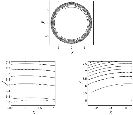
Figure 1: The orbit of a scalar charge with $q^{2}/(\mu M)=0.1$. The upper panel shows the last few orbits before the ISCO. The solid (dashed) line is the orbit to $O(1)$ [$O(\epsilon^{-1})$]. The lower panels display two enlargements of the same orbits: the one on the left emphasizes the difference in the $r$ values, and the one on the right the difference in phase. Here, $x=(r/M)\cos\phi$ and $y=(r/M)\sin\phi$.

As currently we do not know $f^{(1)}_{i}$ for gravitational RR, we specialize next to scalar field RR. [When $f^{(1)}_{i}$ are obtained for gravitational RR in any regular gauge, the analysis below can be repeated for that case.] Specifically, we study the model of a scalar charge $q$ of mass $\mu$, which in the absence of self interaction moves along a circular and equatorial geodesic around a Schwarzschild black hole of mass $M$. For this model, the local SF was computed recently in Refs. burko-00 ; detweiler . The scalar field $\Phi$ satisfies the wave equation $\square\Phi=-4\pi\rho$, where $\rho$ is the scalar charge density. Solving this equation for the appropriate motion in Schwarzschild spacetime (see Ref. burko-00 for details), we obtain the bare SF by ${{}^{\rm bare}f}_{\mu}^{\rm SF}=q\partial_{\mu}\Phi$. The bare force ${{}^{\rm bare}f}_{\mu}^{\rm SF}$ can be regularized using mode-sum regularization, a procedure which yields the physical, finite part of the SF, $f_{\mu}^{\rm SF}$.

We next choose $\epsilon=0.1$, and integrate to find the orbit. We started from $r_{\rm initial}=30M$ and integrated inward toward the innermost stable circular orbit (ISCO) at $r=6M$. (We do not consider the correction to the location of the ISCO, which is irrelevant to the question of interest here.) At intermediate points along the orbit we evaluated $f_{\mu}^{\rm SF}$ and ${f_{\mu}^{\rm SF}}^{\prime}$ using a best fit to a smooth function. Our results are displayed in Fig. 1. We find that the orbit to $O(1)$ decays slower than the orbit to $O(\epsilon^{-1})$. This is indeed expected, as $f_{r}^{(1)}$, which does not contribute at $O(\epsilon^{-1})$, is a repulsive force, which slows down the decay of the orbit. Note, that because our correction to the orbit is at $O(1)$, the last few revolutions look qualitatively the same also for other choices of $\epsilon$.

comp1.eps

Figure 2: The magnitude of the higher-order corrections. Upper panel: $\Delta\left(\frac{V}{r\omega}\right)/\left(\frac{V}{r\omega}\right)^{2}$ as a function of $r$. The solid line is the full effect, the dotted (dashed) line is the contribution of the term in Eq. (8) proportional to $\sigma_{(1)}$ [$V_{(2)}$]. Lower panel: $\Delta\,d{\cal N}_{\rm cyc}/\,d(\ln f)$ as a function of $r$. The solid line is the full effect. The dotted line is the contribution of the term in Eq. (7) proportional to $\sigma_{(1)}^{\prime}$, and the lower (upper) dashed line the contribution of the term proportional to $\sigma_{(1)}$ [$V_{(2)}$].

We next study the magnitude of the higher-order effect by considering Eqs. (7) and (8). Figure 2 shows $\Delta\,d{\cal N}_{\rm cyc}/\,d(\ln f)$ and $\Delta\left(\frac{V}{r\omega}\right)/\left(\frac{V}{r\omega}\right)^{2}$. We first notice that both are dominated by the terms in the corresponding equations proportional to $V_{(2)}$. In fact, at the ISCO the other terms vanish, such that at the ISCO these quantities are fully described by the terms proportional to $V_{(2)}$. (Strictly speaking, the ISCO may be defined by the requirement that $\,d{\cal N}_{\rm cyc}/\,d(\ln f)$ vanishes. As noted above, we do not consider here the shift in the location of the ISCO, and our previous remarks relate, in fact, to $r=6M$, not the ISCO proper. Note also that it is important to evaluate $V_{(2)}$: the effect is controlled by that term at and near $r=6M$.) Fitting our results, we find that $\Delta\,d{\cal N}_{\rm cyc}/\,d(\ln f)\sim D\,f^{\frac{8}{9}}$, where $D\approx 5.9$. Integrating from $r_{\rm start}=20M$ down to $r=6M$, we find that the $O(\epsilon^{-1})$ template would slip by about a tenth of a cycle compared with the data stream. This magnitude is independent of $\epsilon$. $V/(r\omega)$, however, is at $O(\epsilon)$. We thus conclude that changes in amplitude will generally be unimportant for small values of $\epsilon$.

waveform3.eps

Figure 3: The waveforms. In all panels the solid (dashed) line describes the waveform to $O(1)$ [$O(\epsilon^{-1})$]. The upper left panel describes the waves from an early part of the orbit. The lower panel describes the last few cycles before the ISCO. The upper right panel is a magnification of the last maximum.

Finally, we present in Figure 3 the waveforms to $O(1)$ and to $O(\epsilon^{-1})$. We estimate the waveforms by means of the usual “restricted waveform” approximation damour , i.e.,

$$h(t)=C\;v_{\omega}^{2}(t)\cos[\phi_{\rm wave}(t)]\,,$$ (10)

where $v_{\omega}=(\,d\phi/\,dt)^{1/3}$, and $C$ is an amplitude coefficient which depends on the distance of the source of the waves. (For gravitational waves $\phi_{\rm wave}=2\phi$, and that for scalar field waves $\phi_{\rm wave}=\phi$.) Notice that our results above are independent of our adoption of the restricted waveform. The two waveforms are initially in phase. A phase difference, described by Eq. (7) builds up slowly, and is clearly visible in the last few cycles. In addition a difference in amplitude is also clearly seen. The latter effect, however, is an artifact of the relatively large value of $\epsilon$. This change in amplitude decreases linearly with $\epsilon$. The phase shift, on the other hand, is independent of $\epsilon$.

We emphasize that our conclusions are specific to scalar field RR. When gravitational RR is considered, the magnitude of the higher-order effects could be different. For gravitational RR we pick up an obvious factor of $2$ in Eq. (7), such that one may expect the higher-order effect to be even more important for gravitational RR. Determination of $f_{\alpha}^{\rm SF}$ (and its gradients) for gravitational RR is required in order to quantify this effect accurately.

An important issue is the possibility to use templates to $O(\epsilon^{-1})$, to cross correlate against the data stream. One may hope, that templates to $O(\epsilon^{-1})$ for slightly different parameters may be a good approximation, such that one does not have to build templates to $O(1)$. We believe that such an approach may indeed be useful for search purposes. This is in general impossible to do to high accuracy when the cross correlation is done with the full wave train: The waveform is a power series in $\epsilon$, in which there are different functions of $r$ at each order. When one changes $\epsilon$ to correct for the $O(1)$ effects in the waveform, the $O(\epsilon^{-1})$ terms change correspondingly, such that the possibility to fit the template to the data stream by changing $\epsilon$ appears to us to be slim. Indeed, numerical experiments suggest to us that when the parameter space is one dimensional, such techniques are not very useful. [In the scalar field toy model we have, in fact, a two-dimensional parameter space, which includes $q/\mu$ and $\mu/M$, which can be varied independently. In the more realistic case of gravitational RR, however, $q/\mu$, where $q$ is loosely a charge for the gravitational field of $\mu$ (or an active mass), is determined uniquely as unity by the Equivalence Principle. Motivated by the gravitational RR problem, we considered an effective one-dimensional parameter space also for the scalar field toy model, and varied only $q^{2}/(\mu M)$.] On the other hand, when more complicated orbits are concerned (e.g., non-equatorial orbits, when both the particle and the central black hole are spinning), the parameter space will be significantly larger, such that such an approach may be quite successful. Because of the very slow increase in the phase difference between the $O(\epsilon^{-1})$ template and the data stream, it appears to us that data analysis techniques based on dividing the wave train into many chunks, in which the change in phasing is negligible, may be very successful for this problem. However, we emphasize that for realization of the potentially high accuracy gravitational-wave astronomy, one would have to take higher-order corrections, such as those considered here, into consideration.

I thank Steve Detweiler for communicating to me his results before their publication. I thank the participants of the Fifth Capra Ranch Meeting on Radiation Reaction, and in particular Warren Anderson, Scott Hughes, and Amos Ori for comments. I am indebted to Richard Price for invaluable discussions and useful suggestions. This research was supported by the National Science Foundation through grant No. PHY-9734871, and in part through the Center for Gravitational Wave Physics, under Cooperative Agreement PHY-0114375.

References

- (1) For details on the LISA mission see http://lisa.jpl.nasa.gov.
- (2) L. S. Finn and K. S. Thorne, Phys. Rev. D 62, 124021 (2000).
- (3) S. Sigurdsson and M. J. Rees, Mon. Not. R. Astron. Soc. 284, 318 (1997).
- (4) S. A. Hughes, Phys. Rev. D 61, 084004 (2000); D 63, 049902 (2001) (E); D 64 064004 (2001).
- (5) K. Glampedakis and D. Kennefick, gr-qc/0203086.
- (6) C. Cutler et al, Phys. Rev. Lett. 70, 2984 (1993).
- (7) L. M. Burko, Int. J. Mod. Phys. A 16, 1471 (2001).
- (8) S. Detweiler, unpublished.
- (9) L. M. Burko, Phys. Rev. Lett. 84, 4529 (2000).
- (10) S. Detweiler, E. Messaritaki and B. F. Whiting, gr-qc/0205079.
- (11) T. Damour, B. R. Iyer, and B. S. Sathyaprakash, Phys. Rev. D 57, 885 (1998).