An interpretation of Robinson–Trautman type N solutions

Abstract

The Robinson–Trautman type N solutions, which describe expanding gravitational waves, are investigated for all possible values of the cosmological constant $\Lambda$ and the curvature parameter $\epsilon$. The wave surfaces are always (hemi-)spherical, with successive surfaces displaced in a way which depends on $\epsilon$. Explicit sandwich waves of this class are studied in Minkowski, de Sitter or anti-de Sitter backgrounds. A particular family of such solutions which can be used to represent snapping or decaying cosmic strings is considered in detail, and its singularity and global structure is presented.

PACS numbers: 04.20.Jb, 04.30.-w

1 Introduction

The family of Robinson–Trautman solutions [1]–[4] is well known. They are algebraically special solutions having a repeated principal null direction which is associated with an expanding, shear-free and twist-free null geodesic congruence. However, in general, these solutions are still not well understood. A complete physical interpretation is only known for a few very special cases (of type D). It is the purpose of the present paper to clarify the physical meaning of the type N solutions of this class.

These Robinson–Trautman type N solutions can be classified [5], [6] as $RTN(\Lambda,\epsilon)$, where the two constant parameters are the cosmological constant $\Lambda$, and the Gaussian curvature $2\epsilon$ of certain privileged spatial sections. Some physical aspects of these solutions have been investigated in [7] using an analysis of geodesic deviation.

The approach to be adopted in the present paper is as follows: – First we consider the weak field limit in which the metric approaches the background Minkowski, de Sitter or anti-de Sitter space-times. In this limit, it is possible to determine exactly the geometrical properties of the wave surfaces and the locations of the singularities which appear in the metric. After this, we consider an explicit family of exact sandwich wave solutions. Since these propagate into Minkowski, de Sitter or anti-de Sitter backgrounds, the geometry of the wavefronts can again be analysed completely.

In particular, it is found that some sandwich wave solutions of this type may be interpreted in terms of snapping and decaying cosmic strings in the corresponding backgrounds. One simple case of this has been briefly presented [8], but the full family of such solutions in different backgrounds and for different families of wave surfaces and profiles is described here.

The sandwich wave solutions considered here can all be reduced to their impulsive limits. These describe spherical impulsive gravitational waves in backgrounds of constant curvature that are generated by snapping (or expanding) cosmic strings. Such solutions are well known [9]–[19] and can be constructed by various methods in all these backgrounds. It has been observed, however, that these cannot be considered as impulsive Robinson–Trautman solutions in a rigorous sense, as these would involve the square of the delta function appearing in the metric when written in García–Plebański coordinates. Nevertheless, it has recently been argued [16] that these limits are indeed reasonable. The impulsive limits of the sandwich waves presented in [8] and below confirm this. Moreover, they provide a framework in which these limits can be investigated more rigorously.

2 The Robinson–Trautman type N solutions

All Robinson–Trautman solutions of Petrov type N, which are necessarily vacuum but with a possibly non-zero cosmological constant $\Lambda$, are given by the line element

$${\rm d}s^{2}=2\,{\rm d}u\,{\rm d}r+\Big{[}2\epsilon-2r(\log P)_{u}-{\Lambda\over 3}r^{2}\Big{]}{\rm d}u^{2}-2{r^{2}\over P^{2}}\,{\rm d}\zeta\,{\rm d}\bar{\zeta},$$ (1)

where the null coordinate $u$ can be regarded as retarded time, $r$ is a Bondi-type luminosity distance, and $\zeta$ is a complex stereographic-type coordinate. The function $2\epsilon(u)$ is the Gaussian curvature of the 2-surfaces $2P^{-2}{\rm d}\zeta{\rm d}\bar{\zeta}$. A coordinate freedom can always be used to set $\epsilon$ to $+1$, $0$ or $-1$. The function $P(\zeta,\bar{\zeta},u)$ has to satisfy the field equation  $P^{2}(\log P)_{\zeta\bar{\zeta}}=\epsilon$,  which has the general solution [3]

$$P=\big{(}1+\epsilon F\bar{F}\big{)}\big{(}F_{\zeta}\bar{F}_{\bar{\zeta}}\big{)}^{-1/2},$$ (2)

where $F=F(\zeta,u)$ is an arbitrary complex function of $u$ and $\zeta$, holomorphic in $\zeta$. Using a natural tetrad, the only non-zero component of the Weyl tensor is given by

$$\bar{\Psi}_{4}=-{1\over r}\left[P^{2}\big{(}\log P\big{)}_{u\zeta}\right]_{\zeta}={P^{2}\over 2r}F_{\zeta}\left[{1\over F_{\zeta}}\big{(}\log F_{\zeta}\big{)}_{u\zeta}\right]_{\zeta}.$$ (3)

These solutions always contain singular points on each wave surface, which combine to form singular lines, but these are generally not well understood.

It can be seen from (3) that, in the case when $F$ is independent of $u$, the above solution is conformally flat. This is just Minkowski, de Sitter or anti-de Sitter space according to the value of $\Lambda$. Since we will consider sandwich Robinson–Trautman waves below, we will refer to these as background spaces and treat them separately in the next two sections. Although it is obviously not the only possibility, these are the simplest conformally flat limits of these solutions. They correspond to the natural choice of $f(\xi,u)=0$ in the coordinates of [5] (see also [6]).

3 Coordinates in the Minkowski background

Let us first consider the Minkowski metric in the form

$${\rm d}s^{2}=2\,{\rm d}{\cal U}\,{\rm d}{\cal V}-2\,{\rm d}\eta\,{\rm d}\bar{\eta},$$ (4)

in which the coordinates are related to the usual cartesian coordinates by

$${\cal U}={\textstyle{1\over\sqrt{2}}}(t+z),\qquad{\cal V}={\textstyle{1\over\sqrt{2}}}(t-z),\qquad\eta={\textstyle{1\over\sqrt{2}}}(x+iy).$$ (5)

Then the transformation

$${\cal U}=u+{r\,F\bar{F}\over 1+\epsilon F\bar{F}},\qquad{\cal V}=\epsilon u+{r\over 1+\epsilon F\bar{F}},\qquad\eta={r\,F\over 1+\epsilon F\bar{F}},$$ (6)

where  $F=F(\zeta)$  puts the Minkowski metric to the form

$${\rm d}s^{2}=2\,{\rm d}u\,{\rm d}r+2\epsilon\,{\rm d}u^{2}-2{r^{2}\over P^{2}}{\rm d}\zeta{\rm d}\bar{\zeta},$$

where $P$ is given by (2). This is exactly the Minkowski limit of the Robinson–Trautman family of solutions (1) considered above in which $\Lambda=0$ and $F$ is independent of $u$. The inverse transformation is given by

$$u = {\cal U}-{1\over 2\epsilon}\left[\sqrt{({\cal V}-\epsilon\,U)^{2}+4\epsilon\eta\bar{\eta}}-({\cal V}-\epsilon\,{\cal U})\right],$$

$$F(\zeta) = {1\over 2\epsilon\bar{\eta}}\left[\sqrt{({\cal V}-\epsilon\,{\cal U})^{2}+4\epsilon\eta\bar{\eta}}-({\cal V}-\epsilon\,{\cal U})\right],$$ (7)

$$r = \sqrt{({\cal V}-\epsilon\,{\cal U})^{2}+4\epsilon\eta\bar{\eta}},$$

which reduces to  $u={\cal U}-\eta\bar{\eta}/{\cal V}$,  $F=\eta/{\cal V}$,  $r={\cal V}$  in the limit when $\epsilon=0$.

From (7), it follows that the waves surfaces  $u=u_{0}=$ const.  are given by

$$\left(t-{\textstyle{1\over\sqrt{2}}}(1+\epsilon)u_{0}\right)^{2}-x^{2}-y^{2}-\left(z-{\textstyle{1\over\sqrt{2}}}(1-\epsilon)u_{0}\right)^{2}=0.$$

This describes a family of null cones. However, to assist with the physical interpretation that will be presented later, we only consider the family of future null cones relative to each vertex. These are clearly expanding spheres for all values of $\epsilon$ and $u_{0}$. Successive cones are each displaced in the various $t$ and $z$ directions as indicated in the space-time diagrams given in figure 1.

The eps version of this figure is too large to place on the archive. A pdf version of this preprint with all figures is available at www.lboro.ac.uk/departments/ma/preprints/papers02/02-27abs.html

Figure 1: Families of null cones given by  $u=u_{0}$  foliate Minkowski space-time in different ways in the three cases for which $\epsilon=1,0,-1$. (One spatial dimension ($y$) is suppressed).

When  $\epsilon=+1$  all the null cones $u=$ const. naturally fit inside each other and foliate the entire space-time. These surfaces are composed of expanding concentric spheres. In this case, it can be seen from (5) and (7) that the origin of the Robinson–Trautman coordinate $r=0$ corresponds to $x=y=z=0$, with $t$ arbitrary, thus representing all the vertices of the family of cones localised along the $t$ axis.

When  $\epsilon=0$  the cones all have a common line $t=z$, $x=y=0$. The null cones which represent expanding spheres, however, only foliate the half of the Minkowski space given by $t>z$. (The other half, representing contracting spheres, would cover the remaining half $t<z$.) In this case, the origin of the Robinson–Trautman coordinate $r=0$ corresponds to the boundary plane $t=z$, with $x$ and $y$ arbitrary.

When  $\epsilon=-1$,  however, the null cones all intersect each other. In this case, the origin of the Robinson–Trautman coordinate $r=0$ corresponds to  ${t^{2}=x^{2}+y^{2}}$,  with $z$ arbitrary. This clearly represents the envelope of the above family of cones, and is a cylinder which expands at the speed of light. The half null cones representing expanding spheres doubly foliate the inner region $t\geq\sqrt{x^{2}+y^{2}}$. (Similarly, the half null cones representing contracting spheres would doubly foliate the region $t\leq-\sqrt{x^{2}+y^{2}}$). Points for which $|t|<\sqrt{x^{2}+y^{2}}$ are all excluded in these foliations. For the weak field limit of the Robinson–Trautman solutions, an overlapping of the wave surfaces is not permitted. Thus each wave surface for this case must be represented only by a family of half null cones for which $z\geq\sqrt{2}u_{0}$, as indicated in figure 2. This restriction is necessary to maintain a consistent and unambiguous foliation.

The eps version of this figure is too large to place on the archive. A pdf version of this preprint with all figures is available at www.lboro.ac.uk/departments/ma/preprints/papers02/02-27abs.html

Figure 2: Three typical members of the family of null cones $u=$ const. which foliate part of Minkowski space in the case when $\epsilon=-1$. (One spatial dimension ($y$) has been suppressed.)

For the case $\epsilon=-1$, there appears to be another singularity when  $P=0$,  i.e. when  $|F|=1$.  It can be seen from (7) that this occurs for  ${t^{2}=x^{2}+y^{2}}$,  with $z$ arbitrary. However, this exactly coincides with $r=0$, which is the envelope of the null cones discussed above. It can therefore be seen that the parts of null cones $t\geq 0$, $z\geq\sqrt{2}u_{0}$, which are the wave surfaces for this solution, are spanned by the above coordinates with $|F|\leq 1$. (The other half of the cones $z\leq\sqrt{2}u_{0}$ are spanned by $|F|\geq 1$.)

4 Coordinates in the (anti-)de Sitter background

The above analysis of the character of the coordinates applies only to the Minkowski background. However, a similar structure also occurs in de Sitter and anti-de Sitter backgrounds. In these cases, however, it is the global structure which is different.

It is well known that the (anti-)de Sitter space can be represented as a four-dimensional hyperboloid

$${Z_{0}}^{2}-{Z_{1}}^{2}-{Z_{2}}^{2}-{Z_{3}}^{2}-\varepsilon{Z_{4}}^{2}=-\varepsilon a^{2},$$ (8)

embedded in a five-dimensional Minkowski space-time

$${\rm d}s^{2}={\rm d}{Z_{0}}^{2}-{\rm d}{Z_{1}}^{2}-{\rm d}{Z_{2}}^{2}-{\rm d}{Z_{3}}^{2}-\varepsilon{\rm d}{Z_{4}}^{2},$$

where $a^{2}=3/|\Lambda|$ for a cosmological constant $\Lambda$, $\varepsilon=1$ for a de Sitter background ($\Lambda>0$), and $\varepsilon=-1$ for an anti-de Sitter background ($\Lambda<0$). Using the parameterization

$${\cal U}=\sqrt{2}a\,{Z_{0}+Z_{1}\over Z_{4}+a},\qquad{\cal V}=\sqrt{2}a\,{Z_{0}-Z_{1}\over Z_{4}+a},\qquad\eta=\sqrt{2}a\,{Z_{2}+iZ_{3}\over Z_{4}+a},$$ (9)

the metric takes the form

$${\rm d}s^{2}={2\,{\rm d}{\cal U}\,{\rm d}{\cal V}-2\,{\rm d}\eta\,{\rm d}\bar{\eta}\over\left[1+{\Lambda\over 6}(\eta\bar{\eta}-{\cal UV})\right]^{2}},$$ (10)

which is explicitly conformal to Minkowski space (4) to which it reduces when $\Lambda=0$. Applying now the transformation (6), the line element becomes

$${\rm d}s^{2}={2\,{\rm d}u\,{\rm d}r+2\epsilon\,{\rm d}u^{2}-2{r^{2}\over P^{2}}\,{\rm d}\zeta\,{\rm d}\bar{\zeta}\over\left[1-{\Lambda\over 6}u(r+\epsilon u)\right]^{2}}.$$

The further transformation

$$\tilde{r}={r\over 1-{\Lambda\over 6}u(r+\epsilon u)},\qquad\tilde{u}=\int{{\rm d}u\over 1-\epsilon{\Lambda\over 6}u^{2}},$$

yields

$${\rm d}s^{2}=2\,{\rm d}\tilde{u}\,{\rm d}\tilde{r}+\Big{[}2\epsilon-{\Lambda\over 3}\tilde{r}^{2}\Big{]}{\rm d}\tilde{u}^{2}-2{\tilde{r}^{2}\over P^{2}}\,{\rm d}\zeta\,{\rm d}\bar{\zeta},$$ (11)

which is clearly the (anti-)de Sitter background expressed in the Robinson–Trautman form (1).

Let us now consider the wave surfaces $\tilde{u}=\tilde{u}_{0}=$ const. Clearly a constant $\tilde{u}$ implies that $u$ is also a constant. Then, substituting $u=u_{0}$ into (7) and the applying the parameterization (9) gives

$$(1+\epsilon){u_{0}\over\sqrt{2}a}\,Z_{0}-(1-\epsilon){u_{0}\over\sqrt{2}a}\,Z_{1}-\left(\varepsilon+\epsilon{{u_{0}}^{2}\over 2a^{2}}\right)Z_{4}+\left(\varepsilon-\epsilon{{u_{0}}^{2}\over 2a^{2}}\right)a=0,$$ (12)

which is linear in $Z_{i}$, thus representing a family of planes in the 5-dimensional Minkowski space. Their sections through the 4-dimensional hyperboloid (8) give the family of wave surfaces $\tilde{u}=$ const. in the (anti-)de Sitter universe. In fact, these planes are tangent to the hyperboloid. In the following, it will be demonstrated that all the sections are null cones relative to a vertex which is the point at which the plane touches the hyperboloid. For this discussion, it will be convenient to introduce a dimensionless parameter $\alpha$ such that  $\tan({\alpha/2})={u_{0}\over\sqrt{2}\,a}$, or

$$\sin\alpha={2\,{u_{0}\over\sqrt{2}\,a}\over 1+{u_{0}^{2}\over 2\,a^{2}}},\qquad\qquad\cos\alpha={1-{u_{0}^{2}\over 2\,a^{2}}\over 1+{u_{0}^{2}\over 2\,a^{2}}},$$ (13)

which will parameterize the family of wave surfaces.

The de Sitter background

For the case in which $\Lambda>0$ (i.e. $\varepsilon=1$), there are three cases to consider.

We first investigate the case when $\epsilon=1$. Using (12) and the parameter $\alpha$ given by (13), the wave surfaces $u=u_{0}$ are given by the planes  $Z_{0}\sin\alpha-Z_{4}+a\cos\alpha=0$.  Their intersections with the hyperboloid (8) are

$$(Z_{0}\cos\alpha-a\sin\alpha)^{2}=Z_{1}^{2}+Z_{2}^{2}+Z_{3}^{2},$$ (14)

which are a family of null cones with vertices localised on the timelike hyperbola  $Z_{0}=a\tan\alpha$,  $Z_{1}=Z_{2}=Z_{3}=0$,  $Z_{4}=a\sec\alpha$,  which corresponds to the origin of the Robinson–Trautman coordinates  $\tilde{r}=0$.  For this case,  ${u_{0}\over\sqrt{2}\,a}=\tanh{\tilde{u}_{0}\over\sqrt{2}\,a}$.  From this it follows that  $\tilde{u}_{0}\in(-\infty,\infty)$  corresponds to the range  $\alpha\in(-{\pi\over 2},{\pi\over 2})$.  Thus, all the vertices are located on an infinite timelike hyperbola with  $Z_{0}\in(-\infty,\infty)$.  The future null cones from these vertices naturally foliate the half of the de Sitter space for which  $Z_{0}+Z_{4}\geq 0$.  These are illustrated in figure 3a.

The eps version of this figure is too large to place on the archive. A pdf version of this preprint with all figures is available at www.lboro.ac.uk/departments/ma/preprints/papers02/02-27abs.html

Figure 3: Families of null cones in de Sitter space given by  $u=u_{0}$  are sections of a hyperboloid in a 5-dimensional Minkowski space. With two dimensions ($Z_{2}$ and $Z_{3}$) suppressed, they appear as straight (null) lines. These foliate parts of the hyperboloid in different ways for the three cases in which $\epsilon=1,0,-1$. The vertices are located respectively along timelike, null and spacelike lines.

Next, we consider the case $\epsilon=0$, for which the wave surfaces are given by the planes  $Z_{4}-a={u_{0}\over\sqrt{2}\,a}(Z_{0}-Z_{1})$.  In this case, their intersections with the hyperboloid are given by

$$\left(Z_{0}-{\textstyle{u_{0}\over 2\sqrt{2}\,a}}(Z_{4}+a)\right)^{2}=\left(Z_{1}-{\textstyle{u_{0}\over 2\sqrt{2}\,a}}(Z_{4}+a)\right)^{2}+Z_{2}^{2}+Z_{3}^{2}.$$ (15)

Again, this is a family of null cones but with vertices now located along one common straight null line  $Z_{0}=Z_{1}={u_{0}\over\sqrt{2}}$,  $Z_{2}=Z_{3}=0$,  $Z_{4}=a$.  However, the origin of the Robinson–Trautman coordinates  $\tilde{r}=0$  actually occurs on the null hypersurface  $Z_{0}=Z_{1}$,  with  $Z_{2}^{2}+Z_{3}^{2}+Z_{4}^{2}=a^{2}$,  which is a sphere with radius $a$ equal to that of the universe at the instant $Z_{0}=0$. For this case,  $u_{0}=\tilde{u}_{0}\in(-\infty,\infty)$  covers the complete null line. The future null cones from the vertices foliate the half of the de Sitter space for which  $Z_{0}-Z_{1}\geq 0$.  These are illustrated in figure 3b.

Finally, we consider the case when $\epsilon=-1$. Again, using (12) and the parameter $\alpha$ from (13), the wave surfaces $u=u_{0}$ are given by the planes  $Z_{1}\sin\alpha+Z_{4}\cos\alpha-a=0$.  Their intersections with the hyperboloid are

$$Z_{0}^{2}=(Z_{1}\cos\alpha-Z_{4}\sin\alpha)^{2}+Z_{2}^{2}+Z_{3}^{2},$$ (16)

which are a family of null cones with vertices on the spacelike circle  $Z_{0}=Z_{2}=Z_{3}=0$,  $Z_{1}=a\sin\alpha$,  $Z_{4}=a\cos\alpha$.  These are illustrated in figure 3c. For this case,  ${u_{0}\over\sqrt{2}\,a}=\tan{\tilde{u}_{0}\over\sqrt{2}\,a}$,  so that  $\alpha={\sqrt{2}\,\tilde{u}_{0}\over a}$.  It is therefore necessary that  $\tilde{u}_{0}\in(-{a\pi\over\sqrt{2}},{a\pi\over\sqrt{2}}]$,  or  $\alpha\in(-\pi,\pi]$.  Thus, the vertices are located on a closed circle around the de Sitter universe with  $Z_{0}=Z_{2}=Z_{3}=0$.  However, in this case, the future null cones from these vertices would cover the future half  ($Z_{0}\geq 0$)  of the de Sitter space twice. As for the Minkowski case with $\epsilon=-1$, again we must only consider the family of half null cones with  $Z_{1}\geq Z_{4}\tan\alpha$.  Locally these are similar to the wave surfaces illustrated in figure 2 but, in this case, they wrap round the entire universe. Moreover, the origin  $\tilde{r}=0$  now corresponds to  $Z_{0}^{2}=Z_{2}^{2}+Z_{3}^{2}$  with  $Z_{1}^{2}+Z_{4}^{2}=a^{2}$.  When $Z_{0}=0$, this is the closed circle around the de Sitter universe containing all the vertices of the null cones. For $Z_{0}>0$, this a torus $S^{1}\times S^{1}$. Thus, in this case, the origin of the Robinson–Trautman coordinates is a torus whose radius expands at the speed of light in the de Sitter background. We finally observe that the apparent singularity which occurs when $P=0$ coincides exactly with this expanding toroidal origin $\tilde{r}=0$.

The anti-de Sitter background

For the alternative case in which $\Lambda<0$ (i.e. $\varepsilon=-1$), there are again three cases to consider.

First, when $\epsilon=1$, the wave surfaces $u=u_{0}$ are given by the planes  $Z_{0}\sin\alpha+Z_{4}\cos\alpha-a=0$.  Their intersections with the hyperboloid are

$$(Z_{0}\cos\alpha-Z_{4}\sin\alpha)^{2}=Z_{1}^{2}+Z_{2}^{2}+Z_{3}^{2},$$ (17)

which are null cones with vertices on the closed timelike line  $Z_{0}=a\sin\alpha$,  $Z_{1}=Z_{2}=Z_{3}=0$,  $Z_{4}=a\cos\alpha$  in the anti-de Sitter universe. This line corresponds to the origin of the Robinson–Trautman coordinate  $\tilde{r}=0$.  Again in this case,  $\alpha={\sqrt{2}\,\tilde{u}_{0}\over a}$,  so that  $\tilde{u}_{0}\in(-{a\pi\over\sqrt{2}},{a\pi\over\sqrt{2}}]$  corresponds to  $\alpha\in(-\pi,\pi]$.  The future null cones from these vertices, which are illustrated in figure 4a, now cover the complete anti-de Sitter space. It is also possible to consider the covering space for which $\tilde{u}_{0}$ is permitted to take any value.

The eps version of this figure is too large to place on the archive. A pdf version of this preprint with all figures is available at www.lboro.ac.uk/departments/ma/preprints/papers02/02-27abs.html

Figure 4: Families of null cones  $u=u_{0}$  in anti-de Sitter space are sections of a hyperboloid in a 5-dimensional Minkowski space. With the spatial dimensions $Z_{2}$ and $Z_{3}$ suppressed, they are straight (null) lines. These foliate parts of the hyperboloid in different ways for the three cases in which $\epsilon=1,0,-1$, with vertices located respectively along timelike, null and spacelike lines.

Next, when $\epsilon=0$, the wave surfaces are given by the planes  $Z_{4}-a=-{u_{0}\over\sqrt{2}\,a}(Z_{0}-Z_{1})$.  In this case, their intersections with the hyperboloid are the null cones

$$\left(Z_{0}-{\textstyle{u_{0}\over 2\sqrt{2}\,a}}(Z_{4}+a)\right)^{2}=\left(Z_{1}-{\textstyle{u_{0}\over 2\sqrt{2}\,a}}(Z_{4}+a)\right)^{2}+Z_{2}^{2}+Z_{3}^{2}.$$ (18)

with vertices located on one common null line  $Z_{0}=Z_{1}={u_{0}\over\sqrt{2}}$,  $Z_{2}=Z_{3}=0$,  $Z_{4}=a$.  However, the origin of the Robinson–Trautman coordinate  $\tilde{r}=0$  actually occurs on the null hypersurface  $Z_{0}=Z_{1}$  with  $Z_{4}^{2}=a^{2}+Z_{2}^{2}+Z_{3}^{2}$,  which is a hyperboloidal surface. With  $u_{0}=\tilde{u}_{0}\in(-\infty,\infty)$,  the future null cones foliate the half of the anti-de Sitter space for which  $Z_{0}-Z_{1}\geq 0$.  These are illustrated in figure 4b.

Finally, when $\epsilon=-1$, the wave surfaces $u=u_{0}$ are given by the planes  $Z_{1}\sin\alpha-Z_{4}+a\cos\alpha=0$,  which intersect the hyperboloid on the null cones

$$Z_{0}^{2}=(Z_{1}\cos\alpha-a\sin\alpha)^{2}+Z_{2}^{2}+Z_{3}^{2}.$$ (19)

These are illustrated in figure 4c. Their vertices are located on the spacelike hyperbola  $Z_{0}=Z_{2}=Z_{3}=0$,  $Z_{1}=a\tan\alpha$,  $Z_{4}=a\sec\alpha$.   For this case,  ${u_{0}\over\sqrt{2}\,a}=\tanh{\tilde{u}_{0}\over\sqrt{2}\,a}$.  Here again  $\tilde{u}_{0}\in(-\infty,\infty)$  corresponds to  $\alpha\in(-{\pi\over 2},{\pi\over 2})$,  so that  $Z_{1}\in(-\infty,\infty)$.  As for the previous cases in which $\epsilon=-1$, to provide an unambiguous foliation, we must again only consider the family of half null cones with  $Z_{1}\geq a\tan\alpha$,  which are analogous to the wave surfaces illustrated in figure 2. Moreover, the origin  $\tilde{r}=0$  of the Robinson–Trautman coordinates corresponds to  $Z_{0}^{2}=Z_{2}^{2}+Z_{3}^{2}$  with  $Z_{4}^{2}=a^{2}+Z_{1}^{2}$.  When $Z_{0}=0$, this is a hyperbola across the anti-de Sitter universe which contains all the vertices of the null cones. For $Z_{0}>0$, it is an expanding cylindrical-type surface $S^{1}\times H^{1}$ centred on this hyperbola. We again observe that the singularity $P=0$ coincides exactly with $\tilde{r}=0$.

5 A class of Robinson–Trautman solutions

The family of all type N Robinson–Trautman solutions (1) are characterised by two parameters $\Lambda$ and $\epsilon$, and an arbitrary holomorphic function $F(\zeta,u)$. To investigate these space-times and their physical interpretation, it is convenient to restrict attention to the particularly simple case in which

$$F(\zeta,u)=\zeta^{g(u)},$$ (20)

where $g(u)$ is an arbitrary positive function of retarded time. For this choice, the expressions involving $P$ given by (2), which appear in the metric (1), take the forms

$$P^{2}={\left[1+\epsilon(\zeta\bar{\zeta})^{g}\right]^{2}\over g^{2}(\zeta\bar{\zeta})^{g-1}}\ ,\qquad(\log P)_{u}=-{\>g^{\prime}\over g}\left(1+{\textstyle{1\over 2}}\log(\zeta\bar{\zeta})^{g}\left[{1-\epsilon(\zeta\bar{\zeta})^{g}\over 1+\epsilon(\zeta\bar{\zeta})^{g}}\right]\right),$$ (21)

and the explicit expression for $\Psi_{4}$ given by (3) is

$$\bar{\Psi}_{4}=-{g^{\prime}\bar{\zeta}\over 2g\,\zeta\,r}\left({1\over|\zeta|^{g}}+\epsilon|\zeta|^{g}\right)^{2}\ .$$ (22)

Obviously, the solution is conformally flat (i.e. the Minkowski, de Sitter or anti-de Sitter backgrounds) if and only if $g$ is a constant. In general it represents an exact gravitational wave with arbitrary amplitude. It reduces to a weak radiation field if $g$ is approximately constant, i.e. when $g^{\prime}/g$ is small. Notice that, interestingly, the term $(\log P)_{u}$ which appears in the metric and the Weyl tensor component $\Psi_{4}$ are both proportional to the same wave profile $g^{\prime}/g$.

Since $\Psi_{4}$ is the only non-vanishing component of the Weyl tensor, it is clear that all the familiar scalar polynomial invariants vanish. These solutions therefore do not contain scalar polynomial curvature singularities. However, a second order invariant for expanding type N space-times has been found by Bičák and Pravda [20]. This is given by

$$I=(48\,\rho^{2}\bar{\rho}^{2}\Psi_{4}\bar{\Psi}_{4})^{2},$$

where $\rho=1/r$ in this case. It follows that the above solutions possess curvature singularities when $r=0$ and when $\zeta=0$ or $\infty$, provided $g^{\prime}\neq 0$. Some aspects of these singularities will be discussed in detail below.

6 Sandwich Robinson–Trautman waves

A particular sandwich Robinson–Trautman wave of the above form has recently been presented in [8] for the case $\Lambda=0$ and $\epsilon=1$. This has the form (20) with

$$g(u)=\left\{\begin{array}[]{lll}1-ab&{\rm for}\ u<0\\ \vskip 3.0pt plus 1.0pt minus 1.0pt\cr 1-a(b-u)&{\rm for}\ 0\leq u\leq b\\ \vskip 3.0pt plus 1.0pt minus 1.0pt\cr 1&{\rm for}\ u>b\end{array}\right.$$ (23)

where $a$ and $b$ are positive constants. This solution represents a Robinson–Trautman wave confined to the region  $0\leq u\leq b$,  in which $g^{\prime}=a$. It has an expanding spherical wavefront $u=0$, and the wave continues until $u=b$, which is also a concentric expanding sphere. Ahead of and behind this wave zone, the space-time is the locally flat Minkowski background. However, taking  $\arg\zeta\in[0,2\pi)$,  the Minkowski region ahead of the wave contains a topological defect localised at $\zeta=0$ and $\zeta=\infty$. This can be interpreted as a cosmic string with the deficit angle $2\pi ab$. By contrast, the Minkowski region behind the wave contains no such defect. This solution has thus been interpreted as representing a snapping cosmic string in a Minkowski background in which the tension (deficit angle) of the string reduces uniformly to zero over a finite interval of retarded time. This decay of the cosmic string may be considered to generate the gravitational wave.

The above solution can be generalised to arbitrary functions $g(u)$, and to all possible values of $\Lambda$ and $\epsilon$. Obviously, $g(u)$ specifies the wave profile, $\Lambda$ determines the background, and $\epsilon$ characterises the geometrical properties of the wave surfaces.

First, it can be seen that on any wave surface $u=$ const., the complex number $F=\zeta^{g}$ represents a stereographic-type coordinate. Introducing the parameterisations,

$$\zeta^{g}=\left\{\begin{array}[]{lll}\cot({\textstyle{1\over 2}}\theta)\,e^{i\phi}&{\rm for}\ \epsilon=1\\ \vskip 3.0pt plus 1.0pt minus 1.0pt\cr{\textstyle{1\over 2}}\varrho\,e^{i\phi}&{\rm for}\ \epsilon=0\\ \vskip 3.0pt plus 1.0pt minus 1.0pt\cr\tanh({\textstyle{1\over 2}}R)\,e^{i\phi}&{\rm for}\ \epsilon=-1\end{array}\right.$$ (24)

the wave surfaces take the standard form

$${4\over P^{2}}\,{\rm d}\zeta\,{\rm d}\bar{\zeta}=\left\{\begin{array}[]{lll}{\rm d}\theta^{2}+\sin^{2}\theta\>{\rm d}\phi^{2}&{\rm for}\ \epsilon=1\\ \vskip 3.0pt plus 1.0pt minus 1.0pt\cr{\rm d}\varrho^{2}+\varrho^{2}\>{\rm d}\phi^{2}&{\rm for}\ \epsilon=0\\ \vskip 3.0pt plus 1.0pt minus 1.0pt\cr{\rm d}R^{2}+\sinh^{2}R\>{\rm d}\phi^{2}&{\rm for}\ \epsilon=-1\end{array}\right.$$ (25)

This is simply the metric on a two-sphere, two-plane, and two-hyperboloid, respectively. (Note that for the case $\epsilon=-1$, we restrict $\zeta$ to the range $|\zeta|\leq 1$ to cover a single sheet of the hyperboloid.) However, if we assume that the argument of $\zeta$ covers the full range $[0,2\pi)$, then $\phi\in[0,2\pi g)$ and these surfaces in general include a deficit angle $2\pi(1-g)$ around $\theta=0$ or $\pi$ if $\epsilon=1$, around $\varrho=0$ if $\epsilon=0$, and around $R=0$ if $\epsilon=-1$.

Clearly, any region in which $g=$ const. must be one of the Minkowski, de Sitter or anti-de Sitter backgrounds according to the value of $\Lambda$. In cases with $g<1$, these regions contain a constant deficit angle on all sections $u=$ const. Together, these are interpreted as forming cosmic strings with constant tension. (If $g>1$, there is an excess angle corresponding to a strut of constant compression.) When $g=1$ there is no string.

In general, in any region in which $g(u)$ is not constant, this is a Robinson–Trautman type N solution, and the deficit angle on each wave surface will vary. However, it can be seen from (22) that the poles about which there is a deficit angle actually correspond to curvature singularities in the Weyl tensor.

By combining the above two possibilities, we can construct solutions in which $g$ is non-constant only over a finite range of $u$. Such solutions clearly represent sandwich Robinson–Trautman waves. The situation in which $g(u)$ is constant ($<1$) in front of the wave and then increases continuously to 1 behind the wave can be interpreted as a disintegrating string (the deficit angle reduces continuously to zero). One particular case of this, described in [8] for $\epsilon=1$, is represented by (23) and illustrated in figure 5a. The analogous solutions for alternative values of $\epsilon$ are also illustrated in figure 5.

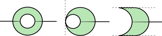
$$\epsilon=1\hskip 108.0pt\epsilon=0\hskip 108.0pt\epsilon=-1$$

Figure 5: The shaded regions represent Robinson–Trautman sandwich waves at some fixed time for different values of $\epsilon$. The expanding spherical (hemispherical for $\epsilon=-1$) wave surfaces are given by $u=$ const. The region behind the wave is Minkowski or (anti-)de Sitter, while the region ahead of the wave is Minkowski or (anti-)de Sitter with a deficit angle representing a cosmic string. The dashed lines denote the boundaries of the coordinate system adopted.

As explained in sections 3 and 4, when $\epsilon=1$ the wave surfaces $u=$ const. at any time are a family of concentric spheres. For the above example, the background space ahead of the wave contains strings of equal tension at opposite sides of the expanding spherical wavefront at $\theta=0$ and $\theta=\pi$.

In the case when $\epsilon=0$, there is only a single pole in $\varrho=0$. The background region thus contains a single string, but only part of the complete space-time is now covered by the coordinate system (that to the right of the dashed line in figure 5b). At any time, the spherical wave surfaces contain a common point, opposite to the pole, as may be observed from the family of null cones in figure 1b.

When $\epsilon=-1$, since we have made the restriction $|\zeta|\leq 1$ here to span only hemispherical surfaces, there is only a single pole $R=0$ on each expanding hemisphere. This may again be attached to a cosmic string in the background region ahead of the wavefront. As explained in previous sections, the envelope of these surfaces $r=0$ is a physical singularity within the wave zone. In the background space-time, it is a cylindrical surface of finite length whose radius is expanding at the speed of light. Its section is denoted by the two thick wavy line in figure 5c. The boundary of the coordinate system is again illustrated in figure 5c by the dashed line.

For the particular choice of the sandwich wave (23), the function $g(u)$ is linear within the wave zone. This gives rise to discontinuities in $\Psi_{4}\sim g^{\prime}(u)$ at $u=0$ and $u=b$, see (22), which correspond to shocks on the boundary wave surfaces indicated in figure 5. However, for this example, the $(\log P)_{u}$ term contained in the metric is also discontinuous on these shock fronts, see (21). (It may be noted that shock Robinson–Trautman waves which have a continuous metric form have been obtained by Nutku [21], but these are not considered further here.) Of course, more general families of sandwich waves without discontinuities in the metric and $\Psi_{4}$ can easily be constructed by permitting $g$ to vary arbitrarily over only a finite range of the retarded time. In this way, we can obtain explicit solutions in which $\Psi_{4}$ may be an arbitrarily smooth function of $u$. In addition, it is particularly interesting to note that, if $g=1$ on both sides of the sandwich, the background does not contain a cosmic string either in front of or behind the wave.

7 The character of singularities and global structure

The illustrations in figure 5 are useful for identifying the location of cosmic strings in the outer region and of string-like structures which are their continuations in the wave zones. However, as can be seen from (22), with $g^{\prime}\neq 0$, these string-like structures at $\zeta=0$ (and $\zeta=\infty$ for $\epsilon=1$) in the wave regions are space-time curvature singularities. These singularities propagate at the speed of light along with the sandwich wave.

In addition, these space-times also always contain singularities when $r=0$. These may naturally be considered as the sources of the Robinson–Trautman solutions. The character of the coordinate origin $r=0$ in the background space-times for different values of $\epsilon$ and $\Lambda$ has already been discussed in sections 3 and 4. For sandwich Robinson–Trautman waves, this curvature singularity occurs only within the wave zones, and does not extend to the regions in front of and behind the waves where $g^{\prime}=0$. The location of this singularity for sections of constant $\zeta$ and different values of $\epsilon$ are illustrated in the space-time pictures in figure 6.

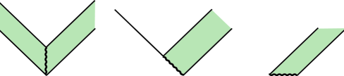
$$\epsilon=1\hskip 96.0pt\epsilon=0\hskip 96.0pt\epsilon=-1$$

Figure 6: Schematic space-time pictures for constant $\zeta$ for Robinson–Trautman sandwich waves with different values of $\epsilon$. The shaded areas are the wave regions. The thick wavy lines represent the singularities at $r=0$. If the particular section corresponds to $\zeta=0$, the region external to the wave also contains a cosmic string which is extended as a string-like singularity through the wave zone.

It should be noted that figure 5 corresponds to a spacelike section through the space-time pictures in figure 6 with the addition of one spatial dimension. The particular section in figure 5 is at a sufficiently late time to contain the complete sandwich. Earlier spacelike sections than those shown in figure 5 could intersect the naked curvature singularity at $r=0$, which corresponds to the source of the wave.

For the cases in which $\epsilon=1$ and $\epsilon=0$, the curvature singularity at $r=0$ corresponds to a timelike or null line respectively, at least in the weak field limit. However, for the case in which $\epsilon=-1$, at an initial time this is a spacelike line of finite length. This line subsequently becomes a cylinder whose radius expands at the speed of light. For a sandwich wave, this expanding cylinder has constant finite length.

For the case in which $\epsilon=1$, the solution can be interpreted as representing the snapping of a cosmic string in which the deficit angle of the string reduces to zero through a region in which it generates the gravitational wave.

A similar interpretation can be given for the case when $\epsilon=0$. However, there is now a boundary of the coordinate systems which is represented as a dashed line in figure 5b. This is a null plane in the background and, as such, it is possible to locally extend the space-time to include an external conformally flat background region. Such an extension is non-unique as an arbitrary impulsive gravitational wave may occur on this null hypersurface. In the absence of such an impulsive wave, it is necessary to have the same backgrounds which contain strings in both directions: i.e. the region to the left of the dashed line in figure 5b is taken to be the same as the region external to the wavefront, having a string with the same deficit angle. In this case, one end of the string is a clean break, while the deficit angle at the other end reduces to zero over a finite range.

The situation when $\epsilon=-1$ is even more complicated. However, a model for a snapping and disintegrating cosmic string can again be obtained by considering two separate sandwich waves of the type described above and illustrated in figures 5c and 6c. These can be combined in such a way that the hemispherical waves propagate in opposite directions as illustrated in figure 7. This enables us to construct a solution in which an initial cosmic string, at an initial time and for some finite section, becomes a curvature singularity. This cylindrical singularity subsequently expands radially at the speed of light (perpendicular to the string) while maintaining constant length. This generates expanding hemispherical gravitational waves at both ends. The deficit angle of the string may reduce to zero through the finite sandwich wave regions in both directions. This would leave an expanding spherical region of the background space-time between the ends of the strings and inside the expanding singular cylinder. This construction, however, requires at least three separate coordinate patches: one representing each of the two sandwich waves, and one to represent the background region external to the expanding cylinder (exterior to the dashed lines in figure 5c).

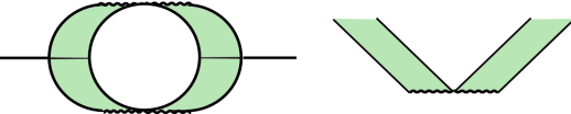
Figure 7: A snapping cosmic string in the case $\epsilon=-1$. The left picture represents the situation at a fixed time (one spatial direction is suppressed). The right picture is a space-time diagram with two spatial directions suppressed. The shaded areas are the wave regions. The thick wavy lines represent the expanding cylindrical singularity where $r=0$.

The properties described above can all be naturally interpreted in a Minkowski background for the case in which $\Lambda=0$. When $\Lambda\neq 0$, the geometry of the sandwich waves illustrated in figure 5 remains basically the same. It is only the geometry of the background which significantly differs. In particular, the snapping straight string in a Minkowski background is replaced by a closed string around the de Sitter universe which snaps at a single event, or an infinite snapping string in an anti-de Sitter background. The structures of the singularity $r=0$ also naturally carry over when $\Lambda\neq 0$ if $\epsilon=1$ or $\epsilon=0$. For $\epsilon=-1$ the expanding cylindrical section is replaced by an expanding section of a torus $S^{1}\times S^{1}$ for $\Lambda>0$, and an expanding section of the surface $S^{1}\times H^{1}$ for $\Lambda<0$.

The pictures in figure 6 also remain valid for any value of $\Lambda$, and it is possible to use these as parts of complete conformal diagrams. However, these would involve including conformal boundaries representing null infinity which has a null, spacelike or timelike character according as $\Lambda=0$, $\Lambda>0$ or $\Lambda<0$ respectively.

8 Further observations

We have presented an explicit family of Robinson–Trautman type N solutions $RTN(\Lambda,\epsilon)$ given by (20). This has proved to be very suitable for the physical interpretation of these solutions. In particular, it has enabled us to construct sandwich waves of this class and to analyse their geometrical properties and the character of the singularities. These all have (hemi-)spherical wave surfaces and propagate in Minkowski, de Sitter or anti-de Sitter backgrounds.

For all the sandwich waves described above, it is straightforward to construct their corresponding impulsive limits. These are obviously expanding spherical impulsive waves which are well known in Minkowski and (anti-)de Sitter backgrounds [9]–[19]. It has been argued [9], [16] that these are impulsive limits of Robinson–Trautman type N solutions, but this limit can here be performed explicitly, without incurring any of the expected difficulties of dealing with the square of a Dirac delta function in the metric.

To construct an impulse on the wave surface $u=u_{0}$, the value of $g$ is simply taken to contain a step function $\Theta(u-u_{0})$, so that $\Psi_{4}\sim\delta(u-u_{0})$. This construction necessarily gives rise to deficit angles in one region or the other, so that such solutions can be interpreted as snapping or expanding cosmic strings. Moreover, it is possible to consider two (or more) sandwich waves, each in their impulsive limits, so that $g\to 1+a\Theta(u-u_{0})-a\Theta(u-u_{1})$, such that the background ahead of the first impulse and behind the second impulse contain no strings (an outline of this has been proposed in [12]). In this sense, a pair of string sections appear and propagate in opposite directions at the speed of light.

The initial ansatz (20) may also be generalised. For example putting

$$F(\zeta,u)=\Big{(}\zeta-h(u)\Big{)}^{g(u)},$$

where $h(u)$ is a complex function, gives rise to the Weyl tensor component

$$\bar{\Psi}_{4}=-{1\over 2r}{(\bar{\zeta}-\bar{h})\over(\zeta-h)}\left({g^{\prime}\over g}+h^{\prime}{\,1-g^{-2}\over\zeta-h}\right)\left({1\over|\zeta-h|^{g}}+\epsilon|\zeta-h|^{g}\right)^{2},$$

which reduces to (22) when $h=0$. This indicates that the singular point on the spherical wave surfaces varies continuously from one surface to another. This would cause the string-like singularity to bend within the wave region. Other functions could introduce additional singular points so that, for example, string-like singularities could even bifurcate. Such behaviour of course depends on the specific character of the holomorphic function $F(\zeta,u)$.

The above solutions, however, are obviously not complete since they do not contain their own past. They only describe the future of events like snapping and disintegrating strings without providing any reasons for those strings to snap or decay.

A remarkable feature of the Robinson–Trautman family of solutions is that they place no restrictions at all on the character and decay of string-like structures of the type described above. Any form of snapping or decaying string could be accommodated within this framework.

This paper is due to appear in Classical and Quantum Gravity 19 (2002). It is also available, with all figures included, in pdf format at

www.lboro.ac.uk/departments/ma/preprints/papers02/02-27abs.html

References

- [1] Robinson I and Trautman A 1960 Phys. Rev. Lett. 4 431
- [2] Robinson I and Trautman A 1962 Proc. Roy. Soc. A 265 463
- [3] Foster J and Newman E T 1967 J. Math. Phys. 8 189
- [4] Kramer D, Stephani H, MacCallum and Herlt E 1980 Exact solutions of Einstein’s field equations (Cambridge University Press)
- [5] García Díaz A and Plebański J F 1981 J. Math. Phys. 22 2655
- [6] Bičák J and Podolský J 1999 J. Math. Phys. 40 4495
- [7] Bičák J and Podolský J 1999 J. Math. Phys. 40 4506
- [8] Griffiths J B and Docherty P 2002 Class. Quantum Grav. 19 L109
- [9] Penrose R 1972 in General Relativity, L. O’Raifeartaigh (ed.), (Clarendon Press, Oxford)
- [10] Gleiser R and Pullin J 1989 Class. Quantum Grav. 6 L141
- [11] Bičák J 1990 Astron. Nachr. 311, 189.
- [12] Nutku Y and Penrose R 1992 Twistor Newsletter No. 34 9
- [13] Hogan P A 1992 Phys. Lett. A 171 21
- [14] Hogan P A 1993 Phys. Rev. Lett. 70 117
- [15] Hogan P A 1994 Phys. Rev. D 49 6521
- [16] Podolský J and Griffiths J B 1999 Class. Quantum Grav. 16 2937
- [17] Podolský J and Griffiths J B 2000 Class. Quantum Grav. 17 1401
- [18] Aliev A N and Nutku Y 2001 Class. Quantum Grav 18 891
- [19] Podolský J and Griffiths J B 2001 Gen. Rel. Grav. 33 83, 105
- [20] Bičák J and Pravda V 1998 Class. Quantum Grav. 15 1539
- [21] Nutku Y 1991 Phys. Rev. D 44 3164