Scattering of a Long Cosmic String by a Rotating Black Hole

Abstract

The scattering of a straight, infinitely long string by a rotating black hole is considered. We assume that a string is moving with velocity $v$ and that initially the string is parallel to the axis of rotation of the black hole. We demonstrate that as a result of scattering, the string is displaced in the direction perpendicular to the velocity by an amount $\kappa(v,b)$, where $b$ is the impact parameter. The late-time solution is represented by a kink and anti-kink, propagating in opposite directions at the speed of light, and leaving behind them the string in a new “phase”. We present the results of the numerical study of the string scattering and their comparison with the weak-field approximation, valid where the impact parameter is large, $b/M\gg 1$, and also with the scattering by a non-rotating black hole which was studied in earlier works.

¹Theoretical Physics Institute, Department of Physics,  University of Alberta,
Edmonton, Canada T6G 2J1

²Department of Astronomy, University of Virginia, P.O.Box 3818,
University Station, Charlottesville, VA 22903-0818

1 Introduction

Study of cosmic strings and other topological defects and their motion in an external gravitational field is an interesting problem. Cosmic strings are topologically stable one-dimensional objects which are predicted by unified theories. Cosmic strings (as well as other topological defects) may appear during a phase transition in the early Universe. A detailed discussion of cosmic strings and other topological defects can be found in the book by Shellard and Vilenkin [1]. Cosmic strings are naturally predicted by many realistic models of particle physics. The formation of cosmic strings helps to successfully exit the inflationary era in a number of the inflation models motivated by particle physics [2, 3]. The formation of cosmic strings is also predicted in the most classes of superstring compactification involving the spontaneous breaking of a pseudo-anomalous $U(1)$ gauge symmetry ( see e.g. [4] and references therein). Recent measurements of CMB anisotropy and especially the position of the acoustic peaks exclude some of the earlier proposed scenarios where the cosmic strings are the main origin of CMB fluctuations. On the other hand, recent analysis shows that a mixture of inflation and topological defects is consistent with current CMB data [5, 6, 7, 8, 9].

A black hole interacting with a cosmic string is a quite rear example of interaction of two relativistic non-local gravitating systems which allows rather complete analysis. This makes this system interesting from pure theoretical point of view. From more ”pragmatic” viewpoint, this system might be a strong source of gravitational waves. But in order to be able to study this effect one needs first to obtain an information on the motion of the string in the black hole background. The situation here is very similar to the case of gravitational radiation from bodies falling into the black hole.

In this paper we consider the scattering of a long cosmic string by a rotating black hole. We assume that a string is thin and its gravitational back reaction can be neglected. If $\eta$ is a characteristic energy scale of a phase transition responsible for a string formation then the thickness of a string is $\rho\sim\eta^{-1}$ while its dimensionless mass per unit length parameter $\mu^{*}=G\mu/c^{2}\sim\eta^{2}$. For example, for GUT strings $\rho_{GUT}\approx 10^{-29}$cm and $\mu^{*}_{GUT}\approx 10^{-6}$, and for the electroweak phase transitions $\rho_{EW}\approx 10^{-14}$cm and $\mu^{*}_{EW}\approx 10^{-34}$. Since $\mu^{*}\ll 1$ one can neglect (at least in the lowest order approximation) effects connected with gravitational waves radiation during the scattering of the string by a black hole.

We assume that the size of the string is much larger then the Schwarzschild gravitational radius $r_{S}=2GM/c^{2}$ of a black hole and its total mass is much smaller than the black hole mass. The latter condition together with $\mu^{*}\ll 1$ means that we can consider a string as a test object. In order to specify the scattering problem we consider the simplest setup, with the string initially far away from the black hole, so that the string has the form of a straight line. We assume that string is initially moving with the velocity ${\bf v}$ towards the black hole and lying in the plane parallel to the rotation axis of the black hole. This plane is located at distance $b$ with respect to the parallel “plane” passing through the rotation axis. In analogy with a particle scattering we call $b$ the impact parameter.

The scattering of a cosmic string by a non-rotating black hole was previously studied both numerically and analytically [10, 11, 12, 13, 14]. For $b\gg r_{S}$ the string moves in the region where the gravitational potential $GM/r$ is always small, and one can use a weak-field approximation where the string equation of motion can be solved analytically [11, 12, 14].

String scattering in the weak field limit can be described in qualitative terms. In the reference frame of the string the gravitational field of the black hole is time dependent and it excites the string’s transversal degrees of freedom. This effect occurs mainly when the central part of the string passes close to the black hole. Since information is propagating along the string at the velocity of light, there always exist two distant regions, ‘right’ and ‘left’, which have not yet felt this excitation. This asymptotic regions of the string continue their motion in the initial plane (‘old phase’). After scattering, when string is moving again far from the black hole, its central part moves again in a plane which is parallel to the initial plane but is shifted below it by a distance $\kappa=2\pi GMv/\sqrt{c^{2}-v^{2}}$ (‘new phase’). There exist two symmetric kink-like regions separating the ‘new’ phase from the ‘old’ one. These kinks move out of the central region with the velocity of light and preserve their form. Besides the amplitude $\kappa$, the kinks are characterized by a width $w$ which depends on the impact parameter and the initial velocity of the string.

In the strong-field limit this picture qualitatively remains the same for string scattering by a Schwarzschild black hole. This problem was analyzed in detail numerically in [11]. In particular, the quantities $\kappa$ and $w$ were found for different values of $b$ and $v$. The numerical calculations in the strong field limit demonstrated also that for special values of the initial impact parameter $b<b_{crit}(v)$ a cosmic string is captured by the black hole. The critical impact parameter for capture by the Schwarzschild black hole was obtained in [10, 13].

In this paper we study of scattering of straight cosmic strings by a rotating black hole. We assume that the initial direction of the string is parallel to the rotational axis of the black hole. Our focus is on the calculation of the same quantities, $\kappa$ and $w$, and to study how black hole rotation modifies the earlier results for a non-rotating black hole. We present here results for string spacetime evolution, real profiles of a string at different external observer times $T$, as well as asymptotic scattering data. Results connected with capture of the string and near-critical scattering will be discussed in another paper.

The paper is organized as follows. Equations for string motion in a curved spacetime and their solutions in the weak field regime are discussed in section 2. Section  3 contains the formulation of the initial and boundary conditions for straight string motion in the Kerr geometry, and the general scheme of the numerical calculations. In section 4 we describe results for strong field scattering of strings in the Kerr spacetime and “real time” profiles of the strings. Section 5 contains information about asymptotic scattering data (displacement parameter and kink profiles) and their dependence on the impact parameter, velocity, and angular velocity of the black hole. Section 6 contains a general discussion. Numerical details are supplied in an appendix.

2 Equations of motion

2.1 String equation of motion

The worldsheet swept by the string in (4D curved background) space-time can be parametrized by a pair of variables $\zeta^{A}$ ($A=0,1$) so that string motion is described by the equation $x^{\mu}={\cal X}^{\mu}(\zeta^{A})$. The dynamics of the string in a spacetime with metric $g_{\mu\nu}$ is described by the Nambu-Goto effective action

$$I_{0}[{\cal X}^{\mu}]=-\mu\int d^{2}\zeta\ \sqrt{-\gamma}\ ,$$ (2.1)

where

$$\gamma_{AB}=g_{\mu\nu}{\cal X}^{\mu}_{,A}\,{\cal X}^{\nu}_{,B}$$ (2.2)

is the induced metric on the worldsheet. The same equations of motion of the string can be derived from the Polyakov’s form of the action [15],

$$I[{\cal X}^{\mu},h_{AB}]=-{\mu\over 2}\,\int d^{2}\zeta\sqrt{-h}h^{AB}\gamma_{AB}\,.$$ (2.3)

We use units in which $G=c=1$, and the sign conventions of [16]. In (2.3) $h_{AB}$ is the internal metric with determinant $h$.

The variation of the action (2.3) with respect to ${\cal X}^{\mu}$ and $h_{AB}$ gives the following equations of motion:

$$\Box{\cal X}^{\mu}+h^{AB}{\Gamma^{\mu}}_{\alpha\beta}{\cal X}^{\alpha}_{,A}{\cal X}^{\beta}_{,B}=0\,,$$ (2.4)

$$\gamma_{AB}-{1\over 2}h_{AB}h^{CD}\gamma_{CD}=0\,,$$ (2.5)

where

$$\Box={1\over\sqrt{-h}}\partial_{A}(\sqrt{-h}h^{AB}\partial_{B})\,.$$ (2.6)

The first of these equations is the dynamical equation for string motion, while the second one plays the role of a constraint.

We fix internal coordinate freedom by using the gauge in which $h_{AB}$ is conformal to the flat two-dimensional metric $\eta_{AB}=\mbox{diag}(-1,1)$. In this gauge the equations of motion for the string have the form

$$\Box{\cal X}^{\mu}+{\Gamma^{\mu}}_{\alpha\beta}\,{\cal X}^{\alpha}_{,A}\,{\cal X}^{\beta}_{,B}\,\eta^{AB}\,=0\,,$$ (2.7)

and the constraint equations are

$$\gamma_{01}=g_{\mu\nu}\frac{\partial{\cal X}^{\mu}}{\partial\tau}\frac{\partial{\cal X}^{\nu}}{\partial\sigma}=0\ ,$$ (2.8)

$$\gamma_{00}+\gamma_{11}=g_{\mu\nu}\left(\frac{\partial{\cal X}^{\mu}}{\partial\tau}\frac{\partial{\cal X}^{\nu}}{\partial\tau}+\frac{\partial{\cal X}^{\mu}}{\partial\sigma}\frac{\partial{\cal X}^{\nu}}{\partial\sigma}\right)\ =0\ .$$ (2.9)

Here, $\tau\equiv\zeta^{0}$, $\sigma\equiv\zeta^{1}$ and $\Box=-\partial^{2}_{\tau}+\partial^{2}_{\sigma}$. These constraints are to be satisfied for the initial data. As a consequence of the dynamical equations they are valid for any later time.

2.2 Weak field approximation

In the absence of the external gravitational field $g_{\mu\nu}=\eta_{\mu\nu}$, where $\eta_{\mu\nu}$ is the flat spacetime metric. In Cartesian coordinates ($T,X,Y,Z$), $\eta_{\mu\nu}=\mbox{diag}(-1,1,1,1)$ and ${\Gamma^{\mu}}_{\alpha\beta}=0$, and it is easy to verify that

$${\cal X}^{\mu}={\cal X}_{0}^{\mu}(\tau,\sigma)\equiv(\tau\cosh\beta,\tau\sinh\beta+X_{0},b,\sigma)\,,$$ (2.10)

$$h_{AB}=\eta_{AB}\equiv\mbox{diag}(-1,1)\,,$$ (2.11)

is a solution of equations (2.4) and (2.5). This solution describes a straight string oriented along the $Z$-axis which moves in the $X$-direction with constant velocity $v=\tanh\beta$. Initially, at ${\tau}_{0}=0$, the string is found at ${\cal X}^{\mu}(0,\sigma)=(0,X_{0},b,\sigma)$. Later when we use this solution as initial data for a string scattering by a black hole, $b$ will play the role of impact parameter. For definiteness we choose $b>0$ and $X_{0}<0$, so that $\beta>0$.

Let us consider how this solution is modified when the straight string is moving in a weak gravitational field. We assume

$$g_{\mu\nu}=\eta_{\mu\nu}+q_{\mu\nu}\,,$$ (2.12)

$${\cal X}^{\mu}(\zeta)={\cal X}_{0}^{\mu}(\zeta)+\chi^{\mu}(\zeta)\,,$$ (2.13)

where $q_{\mu\nu}$ is the metric perturbation and $\chi^{\mu}$ is the string perturbation. By making the perturbation of the equation of motion one gets

$$\Box\chi^{\mu}=f^{\mu}\,,$$ (2.14)

where

$$f^{\mu}=f^{\mu}(\zeta)=-{\Gamma^{\mu}}_{\alpha\beta}({\cal X}_{0})\,{\cal X}_{0,A}^{\alpha}\,{\cal X}_{0,B}^{\beta}\,\eta^{AB}\,.$$ (2.15)

We use Cartesian coordinates here so that ${\Gamma^{\mu}}_{\alpha\beta}$ is simply the Christoffel symbol for $q_{\mu\nu}$.

The linearized constraint equations are

$$\eta_{\mu\nu}\frac{\partial{\cal X}^{\mu}_{0}}{\partial\tau}\frac{\partial\chi^{\nu}}{\partial\sigma}+\eta_{\mu\nu}\frac{\partial\chi^{\mu}}{\partial\tau}\frac{\partial{\cal X}^{\nu}_{0}}{\partial\sigma}+q_{\mu\nu}\frac{\partial{\cal X}^{\mu}_{0}}{\partial\tau}\frac{\partial{\cal X}^{\nu}_{0}}{\partial\sigma}=0\ ,$$ (2.16)

$$2\eta_{\mu\nu}\left(\frac{\partial{\cal X}^{\mu}_{0}}{\partial\tau}\frac{\partial\chi^{\nu}}{\partial\tau}+\frac{\partial{\cal X}^{\mu}_{0}}{\partial\sigma}\frac{\partial\chi^{\nu}}{\partial\sigma}\right)+q_{\mu\nu}\left(\frac{\partial{\cal X}^{\mu}_{0}}{\partial\tau}\frac{\partial{\cal X}^{\nu}_{0}}{\partial\tau}+\frac{\partial{\cal X}^{\mu}_{0}}{\partial\sigma}\frac{\partial{\cal X}^{\nu}_{0}}{\partial\sigma}\right)=0\ .$$ (2.17)

As in the exact non-linear case, if these linearized constraints are satisfied at the initial moment of time $\tau$ they are also valid for any $\tau$ for a solution $\chi^{\mu}$ of the dynamical equations (2.14).

The linearized equations can be used to study string motion in the case where it is far away from the black hole. In this case the gravitational field can be approximated as follows:

$$ds^{2}=-(1-\frac{2M}{R})dT^{2}+(1+\frac{2M}{R})\,(dX^{2}+dY^{2}+dZ^{2})-\frac{4J}{R^{3}}(XdY-YdX)dT\ ,$$ (2.18)

where $R^{2}=X^{2}+Y^{2}+Z^{2}$, and $M$ and $J=aM$ are the mass and angular momentum of the black hole, respectively. In fact this asymptotic form of the metric is valid for any arbitrary stationary localized distribution of matter, provided that the observer is located far from it. In agreement with (2.18) the gravitational field perturbation can be presented as

$$q_{\mu\nu}=q_{\mu\nu}^{N}+q_{\mu\nu}^{LT}\,,$$ (2.19)

where the Newtonian and Lense-Thirring parts are

$$q_{\mu\nu}^{N}=2\varphi\delta_{\mu\nu}\,,\hskip 28.45274pt\varphi={M\over R}\,,\hskip 28.45274ptq_{\mu\nu}^{LT}={4J\over R^{3}}\,\delta^{0}_{(\mu}\,\epsilon_{\nu)\alpha 03}X^{\alpha}\,.$$ (2.20)

Here $\epsilon_{\alpha\beta\gamma\delta}$ is the antisymmetric symbol. The Lense-Thirring part $q_{\mu\nu}^{LT}$ of the metric [16, 17] is produced by the rotation of the source of the gravitational field and it is responsible for frame dragging.

2.3 Newtonian scattering

In the linear approximation we can study the action of each of the parts of the metric perturbations independently. For the Newtonian part one has the following expression for the force $f^{\mu}_{N}$

$$f^{0}_{N} = 2\sinh(\beta)\cosh(\beta)\,,\varphi_{,1}$$ (2.21)

$$f^{1}_{N} = 0\,,$$ (2.22)

$$f^{2}_{N} = -2\sinh^{2}\beta\varphi_{,2}\,,$$ (2.23)

$$f^{3}_{N} = -2\cosh^{2}\beta\varphi_{,3}\ ,$$ (2.24)

and the constraint equations read

$$\chi^{3}_{,\tau}-\cosh\beta\chi^{0}_{,\sigma}+\sinh\beta\chi^{1}_{,\sigma} = 0\,,$$ (2.25)

$$\chi^{3}_{,\sigma}-\cosh\beta\chi^{0}_{,\tau}+\sinh\beta\chi^{1}_{,\tau} = -2\varphi\cosh^{2}\beta\ .$$ (2.26)

The result $f^{1}=0$ means that in the first order approximation the string lies in the $YZ-$plane at any fixed time $\tau=\mbox{const}$. The dynamical equations (2.3) can be easily integrated by using the retarded Green function (see [11]).

We focus now our attention on the behavior of $\chi^{2}$ which describes the string deflection in the plane orthogonal to its motion. It is easy to show that the asymptotic value of $\chi^{2}(\tau\to\infty,\sigma)$ is the same for any fixed $\sigma$. We denote it $b-\kappa$. The following expression is valid for $\kappa$

$$\kappa=-{1\over 2\sinh\beta}\,\int_{\Pi_{0}}\,dX\,dZf^{2}\,,$$ (2.27)

where $\Pi_{0}$ is the two-dimensional worldsheet swept by the string in its motion in the background spacetime. This integral can be easily calculated since

$$\int_{\Pi_{0}}\,dX\,dZ\varphi_{,Y}=2\pi M\,$$ (2.28)

is the flux of the Newtonian field strength through $\Pi_{0}$. Thus we have

$$\kappa=2\pi M\sinh\beta\,.$$ (2.29)

At any late moment of time $\tau$ the central part of the string is a straight line moving in the plane $Y=b-\kappa$, while its far distant parts move in the original plane $Y=b$. These different “phases” are connected by kinks propagating in the direction from the center with the velocity of light. (For details, see [13]). We call $\kappa$ the displacement parameter. Figure 1 shows the Y-direction displacement for the Newtonian scattering as a function of $\tau$ and $\sigma$.

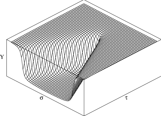
Figure 1: $Y-$profile for Newtonian scattering

2.4 Lense-Thirring scattering

In the presence of rotation the Lense-Thirring force acting on the string in the linearized approximation is

$$f^{0}_{LT} = 6J\sinh^{2}\beta\frac{b(X_{0}+\tau\sinh\beta)}{{\cal R}^{5}}\,,$$ (2.30)

$$f^{1}_{LT} = 0\,,$$ (2.31)

$$f^{2}_{LT} = 2J\sinh\beta\cosh\beta\left(\frac{1}{{\cal R}^{3}}-\frac{3\sigma^{2}}{{\cal R}^{5}}\right)\,,$$ (2.32)

$$f^{3}_{LT} = 6J\sinh\beta\cosh\beta\frac{b\sigma}{{\cal R}^{5}}\,,$$ (2.33)

where ${\cal R}=\sqrt{(X_{0}+\tau\sinh\beta)^{2}+b^{2}+\sigma^{2}}$. As before, $f^{1}=0$.

The constraint equations now take the form

$$\chi^{3}_{,\tau}-\cosh\beta\chi^{0}_{,\sigma}+\sinh\beta\chi^{1}_{,\sigma}=0\,,$$ (2.34)

$$\chi^{3}_{,\sigma}-\cosh\beta\chi^{0}_{,\tau}+\sinh\beta\chi^{1}_{,\tau}=-2J\sinh\beta\cosh\beta\frac{b}{{\cal R}^{3}}\,.$$ (2.35)

The dynamical equations can be solved analytically. For the initial conditions

$$\chi^{0}|_{\tau=0}=0\,,$$ (2.36)

$$\chi^{2}|_{\tau=0}=\frac{\partial\chi^{2}}{\partial\tau}|_{\tau=0}=0\,,$$ (2.37)

$$\chi^{3}|_{\tau=0}=\frac{\partial\chi^{3}}{\partial\tau}|_{\tau=0}=0\,,$$ (2.38)

the solution is

$$\chi^{0}=Jb\sinh\beta\left(\frac{(X_{0}+\tau\sinh\beta)\sinh\beta+\sigma}{\Delta_{(+-)}{\cal R}}+\frac{(X_{0}+\tau\sinh\beta)\sinh\beta-\sigma}{\Delta_{(++)}{\cal R}}\right.\,$$

$$-\left.\frac{X_{0}\sinh\beta-(\tau-\sigma)}{\Delta_{(+-)}\rho_{-}}-\frac{X_{0}\sinh\beta-(\tau+\sigma)}{\Delta_{(++)}\rho_{+}}\right)\,,$$ (2.39)

$$\chi^{1}=0\,,$$ (2.40)

$$\chi^{2}=J\sinh\beta\cosh\beta\left(-\frac{\tau^{2}\sinh^{2}\beta+\tau\sigma\sinh^{2}\beta+2X_{0}\tau\sinh\beta+\sigma X_{0}\sinh\beta+X_{0}^{2}+b^{2}}{\Delta_{(++)}{\cal R}}\right.$$

$$+\frac{-\tau^{2}\sinh^{2}\beta+\tau\sigma\sinh^{2}\beta-2X_{0}\tau\sinh\beta+\sigma X_{0}\sinh\beta-X_{0}^{2}-b^{2}}{\Delta_{(--)}{\cal R}}$$ (2.41)

$$+\left.\frac{X_{0}\sinh\beta(\tau+\sigma)+X_{0}^{2}+b^{2}}{\Delta_{(++)}\rho_{+}}+\frac{X_{0}\sinh\beta(\tau-\sigma)+X_{0}^{2}+b^{2}}{\Delta_{(--)}\rho_{-}}\right)\,,$$

$$\chi^{3}=Jb\sinh\beta\cosh\beta\left(\frac{(X_{0}+\tau\sinh\beta)\sinh\beta-\sigma}{\Delta_{(++)}{\cal R}}-\frac{(X_{0}+\tau\sinh\beta)\sinh\beta+\sigma}{\Delta_{(--)}{\cal R}}\right.$$

$$-\left.\frac{X_{0}\sinh\beta-(\tau+\sigma)}{\Delta_{(++)}\rho_{+}}+\frac{X_{0}\sinh\beta-(\tau-\sigma)}{\Delta_{(--)}\rho_{-}}\right)\,,$$ (2.42)

$$\Delta_{\pm\pm}=(X_{0}\pm(\tau\pm\sigma)\sinh\beta)^{2}+b^{2}\cosh^{2}\beta\,,$$ (2.43)

$$\rho_{\pm}=\sqrt{X_{0}^{2}+b^{2}+(\tau\pm\sigma)^{2}}\,.$$ (2.44)

Using these relations it is possible to see that the displacement parameter $\kappa=\lim_{\tau\to\infty}\,\chi^{2}(\tau,\sigma=0)$ vanishes for this solution. The reason is the following. Using (2.32) it is easy to present $f_{LT}^{2}$ as

$$f_{LT}^{2}=2J\sinh\beta\,\cosh\beta{\partial\over\partial\sigma}\left({\sigma\over{\cal R}^{3}}\right)\,.$$ (2.45)

The asymptotic displacement is given by (2.27). The integral over $Z$ or, equivalently, the integral over $\sigma$ from $f_{LT}^{2}$, which is a total derivative over $\sigma$, reduces to boundary terms $\sigma/{\cal R}^{3}$ at $\sigma=\pm\infty$, which vanish.

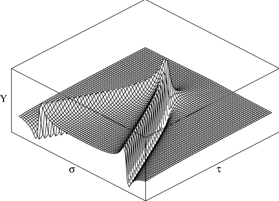
Figure 2: $Y-$profile for Lense-Thirring scattering

Figure 2 shows the $Y-$direction displacement as a function of $\tau$ and $\sigma$ for the weak field scattering. It should be emphasized that the scale of structures for Lense-Thirring scattering is much smaller than that for Newtonian scattering. This can be easily seen if we compare the Newtonian force $f_{N}\sim M/{\cal R}^{2}$ with the Lense-Thirring force $f_{LT}\sim J/{\cal R}^{3}$

$${f_{LT}\over f_{N}}\sim{J\over M{\cal R}}\leq{J\over Mb}\,.$$ (2.46)

For the scattering by a rotating black hole $J=aM$, where $|a|/M\leq 1$ is the rotation parameter. Hence

$${f_{LT}\over f_{N}}\leq{M\over b}\,$$ (2.47)

which is small for the weak field scattering. For this reason, in the weak field regime the string profiles for the prograde or retrograde scattering by rotating black hole do not greatly differ from the profiles for the scattering by a non-rotating black hole of the same mass. The situation is different for strong-field scattering: the displacement parameter is different for prograde and retrograde scattering, and for near-critical scattering the profiles of the kinks contain visible structure produced by effects connected with the rotation of the black hole.

3 String scattering by a Kerr black hole

3.1 String in the Kerr spacetime

Our aim is to study a string motion in the Kerr spacetime. The Kerr metric in Boyer-Lindquist coordinates $(t,r,\theta,\phi)$ has the form

$$ds^{2} = -(1-\frac{2Mr}{\Sigma})dt^{2}+\frac{\Sigma}{\Delta}dr^{2}+\Sigma d\theta^{2}+\frac{A\sin^{2}{\theta}}{\Sigma}d\phi^{2}-\frac{4aMr\sin^{2}{\theta}}{\Sigma}dtd\phi\ ,$$ (3.1)

$$\Sigma = r^{2}+a^{2}\cos^{2}{\theta}\ ,$$ (3.2)

$$\Delta = r^{2}-2Mr+a^{2}\ ,$$ (3.3)

$$A = (r^{2}+a^{2})^{2}-a^{2}\Delta\sin^{2}{\theta}\ ,$$ (3.4)

where $M$ is the mass of the black hole, and $J=aM$ is its angular momentum ($0\leq a\leq M$). At far distances this metric has the asymptotic form (2.18).

In order to be able to deal with the case where part of the string crosses the event horizon for the numerical simulation we adopt the so-called Kerr (in-going) coordinates $(\tilde{v},r,\theta,\tilde{\phi})$

$$ds^{2}=-(1-\frac{2Mr}{\Sigma})d\tilde{v}^{2}+2d\tilde{v}dr-\frac{4aMr\sin^{2}{\theta}}{\Sigma}d\tilde{v}d\tilde{\phi}-a\sin^{2}{\theta}drd\tilde{\phi}$$

$$+\Sigma d\theta^{2}+\frac{A\sin^{2}{\theta}}{\Sigma}d\tilde{\phi}^{2}\ ,$$ (3.5)

with

$$\tilde{v} = t+r+M\ln|{\Delta\over 4M^{2}}|+\frac{M^{2}}{\sqrt{M^{2}-a^{2}}}\ln\left|\frac{r-M-\sqrt{M^{2}-a^{2}}}{r-M+\sqrt{M^{2}-a^{2}}}\right|+M\ ,$$ (3.6)

$$\tilde{\phi} = \phi+\frac{a}{2\sqrt{M^{2}-a^{2}}}\ln\left|\frac{r-M-\sqrt{M^{2}-a^{2}}}{r-M+\sqrt{M^{2}-a^{2}}}\right|\ .$$ (3.7)

The metric (3.1) has the asymptotic form

$$ds^{2}=-dt^{2}+dr^{2}+r^{2}(d\theta^{2}+\sin^{2}\theta d\phi^{2})+\frac{2M}{r}(dt^{2}+dr^{2})-\frac{4aM}{r}\sin^{2}\theta dtd\phi\ .$$ (3.8)

Let us introduce new “quasi-Cartesian” coordinates

$$T = t\ ,$$

$$X = R\sin{\theta}\cos{\phi}\ ,$$

$$Y = R\sin{\theta}\sin{\phi}\ ,$$

$$Z = R\cos{\theta}\ ,$$

where

$$r=R+M\ .$$ (3.9)

One can easily check that the metric (3.8) in the quasi-Cartesian coordinates (3.1) has the asymptotic form (2.18)

It should be emphasized that without the shift (3.9) of the radial coordinate one does not recover (2.18). The reason for this is easy to understand if one considers the same problem for the Schwarzschild geometry. The asymptotic limit of (2.18) with $a=0$ can be found in the isotropic coordinates with $r=\tilde{R}(1+M/2\tilde{R})^{2}$ in which the spatial part of the metric is conformal to the flat metric. Asymptotically, it is sufficient to use (3.9) which is the leading part of $r$ at large $\tilde{R}$.

In what follows we shall use these quasi-Cartesian coordinates for representing the position and the form of the string in the Kerr spacetime even if we are not working in the weak field regime. It should be emphasized that since the space in the Kerr geometry is not flat, plots constructed in these coordinates do not give a “real picture”. This is a special case of a general problem of the visualization of physics in a 4-dimensional curved spacetime.

3.2 Initial and boundary conditions

In an ideal situation, we would study scattering by initially placing our infinitely long string at spatial infinity, where the spacetime is flat and the straight string can be described in simple terms. In a numerical scheme, however, the string cannot be infinitely long and we must start the simulation at a finite distance from the black hole. We discuss here the initial and boundary conditions used for the simulations.

In studying the scattering of a straight string, we consider the special case where the string is initially parallel to the axis of rotation of the black hole. We use Cartesian coordinates in the asymptotic region so that $X$-axis coincides with the direction of motion and the $Z$-axis is along the string (see Fig. 3).

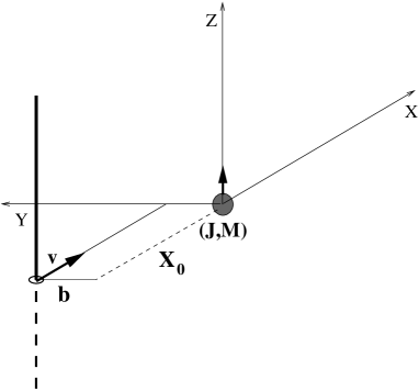
Figure 3: Initial setup of the scattering experiment

We consider a string segment of length $L\sim 10^{4}M$ at a time $\tau_{0}$ and an initial distance $X_{0}$ from the black hole. In order to keep accuracy high and yet prevent the calculation time from being inordinately large, we do not evolve the straight string numerically from this initial position. Instead, we use the weak-field approximation to describe the string configuration at a later time $\tau_{s}$ where the distance $X_{s}$ is closer to the black hole, $|X_{s}|\ll|X_{0}|$  .

Given a sufficiently long string segment, the boundary points move at a great distance from the black hole, so that their evolution can be described by the weak field approximation until information about the interaction with the black hole reaches the boundary. We denote this time as $\tau_{*}$. Starting from this moment we solve the dynamical equations in the region $|\sigma|<L-(\tau-\tau_{*})$ (see figure 4). The larger is the initial value $L$ the longer one can go in $\tau$ in the simulation. We choose $L$ to be large enough to provide the required accuracy in the determining the final scattering data.

Since the boundary conditions found from the weak field regime calculations are not exact there will be disturbance created by this effect. In some cases, when it is important to exclude these disturbances, we used a modified scheme of calculations in which no boundary conditions are used from the very beginning of the simulation. The price for this is that one needs to take longer initial size of $L$ which in turn increases the computational time.

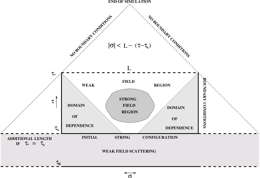
Figure 4: Scheme of time domains for scattering problem

3.3 Solving dynamical equations and constraints

Using the initial conditions at $\tau_{s}$ and boundary conditions we solve numerically the dynamical equations (2.7). Since the equations are of second order, we use the weak-field approximation to get initial data at $\tau_{s}$ and $\tau_{s}+\Delta\tau$ in order to completely specify the initial value problem. The numerical scheme uses second-order finite differences and evolves the string configuration using an implicit scheme. Because of the symmetry $\sigma\to-\sigma$ it is sufficient to evolve only half of the string worldsheet, $\sigma\leq 0$, and use a reflecting boundary condition at the string midpoint. The numerical grid is non-uniform with the denser part following the motion of the kink. We used the constraint equations (2.8-2.9) for an independent check of the accuracy of the calculations. More details on the numerical scheme can be found in the Appendix.

4 String profiles for strong field scattering

4.1 General picture

a	b
c	d

Figure 5: Displacement in $Y-$ direction as a function of $(\tau,\sigma)$ for given velocity $v/c=0.762$ in the weak (a) and strong (b–d) field regime.

Figure 5 demonstrates general features of straight string scattering, here for a string with velocity $v=0.762$ ($\beta=1$). The four panels show the displacement in the $Y-$direction as a function of internal coordinates $(\tau,\sigma)$ for weak and strong field scattering.

Figure 5 (a) shows the scattering for an impact parameter $b=80\,M$. The value of the displacement parameter at the largest $\tau$ shown is $\kappa=7.23M$. This value as well as the form of the kinks are in a very good agreement with the weak-field scattering results. Plots for prograde and retrograde scattering at $b=80\,M$ are virtually indistinguishable from Fig. 5 (a).

Figures 5 (b–d) show the scattering for $b=6\,M$. Qualitatively these plots are similar to weak-field scattering. The main differences are the following: (1) The value of the displacement parameter $\kappa=11.03M$ for the non-rotating black hole is significantly larger then $\kappa=7.23$ for $b=80\,M$. (2) Effects of rotation are more pronounced. The displacement $\kappa$ for retrograde scattering is essentially larger than $\kappa$ for the prograde scattering. (3) The string profile after scattering is more sharp, the width of the kinks is visibly smaller that for weak-field scattering.

4.2 “Real-time profiles” of the string for strong-field scattering

Figure 6: “Real-time profiles” of the string and their $XZ-$ and $YZ-$ projection for the strong field scattering by the Schwarzschild black hole.

Figure 7: “Real-time profiles” of the string and their $XZ-$ and $YZ-$ projection for the strong field retrograde scattering by the extremal Kerr black hole.

Figure 8: “Real-time profiles” of the string and their $XZ-$ and $YZ-$ projection for the strong field prograde scattering by the extremal Kerr black hole.

It should be emphasized that figure 5 give an accurate impression of the displacement effect, but they give a distorted view of the real form of the string. The reason is evident. The grid imposed on the worldsheet is determined by the choice of $(\tau,\sigma)$ coordinates. But a $\tau={\rm const}$ section differs from a time $T={\rm const}$ section in the laboratory slice of spacetime. The position of the string at given time $T$ can be found by using the functions $T(\tau,\sigma)$, $X(\tau,\sigma)$, $Y(\tau,\sigma)$, $Z(\tau,\sigma)$, to find functions $X(T,Z)$ and $Y(T,Z)$. For fixed $T$ these functions determine a position of the string line in 3-space.

Figures 6, 7 and 8 show a sequence of “real-time” profiles for strong-field string scattering at five different coordinate times $T$. We ordered them so that the larger number labeling the string corresponds to later time. In figure 6 the black hole is non-rotating. Figures 7 and 8 show the “real-time” profiles for retrograde and prograde scattering for a maximally rotating black hole, respectively. Again we can see that due to frame dragging, the distortion of the string is more pronounced for retrograde scattering.

5 Late time scattering data

5.1 Displacement parameter

Figure 9: Displacement parameter $\kappa$ as a function of the impact parameter $b$ for different velocities $v$.

Figure 9 shows the dependence of the displacement parameter $\kappa$ on the impact parameter $b$ for different velocities $v$. For a given value of $b$ the curve for $a/M=-1$ always lies higher than the curves for more positive values of $a/M$. This is true for all values of velocity $v$, but this difference is more pronounced at large velocities.

The relative location of the curves for given $v$ and $b$ and different $a$ can be explained by frame dragging. Namely, a string in the retrograde motion is effectively slowed down when it passes near the black hole and hence it spends more time near it. As the result its displacement is greater than the displacement for the prograde motion with the same impact parameter. Let us make order of magnitude estimation of this effect. For this purpose we use metric (2.18). We focus our attention on the Lense-Thirring term and neglect for a moment the Newtonian part. Consider first a point particle moving in this metric with the velocity $v$ and impact parameter $b$. In the absence of rotation it moves with constant velocity so that $(X=vT,Y=b,Z=0)$ and the proper time $\tau$ is

$$\tau_{0}=\sqrt{1-v^{2}}\,T\,.$$ (5.1)

In the presence of rotation one has

$$d\tau^{2}=(1-v^{2})\,dT^{2}-{4Jbv\over R^{3}}\,dT^{2}\,,$$ (5.2)

where

$$R^{2}=b^{2}+v^{2}\,T^{2}\,.$$ (5.3)

For large $b$ one can write

$$\tau=\tau_{0}+\Delta\tau\,,$$ (5.4)

where

$$\Delta\tau=-{2Jbv\over\sqrt{1-v^{2}}}\,\int_{-\infty}^{\infty}\,{dT\over(b^{2}+v^{2}T^{2})^{3/2}}\,=-{4J\over b\sqrt{1-v^{2}}}\,.$$ (5.5)

This quantity $\Delta\tau$ characterize additional time delay for the motion in the Lense-Thirring field. The characteristic time of motion in the vicinity of a black hole is $\tau_{int}\sim b/v$. Thus we have

$${\Delta\tau\over\tau_{int}}\sim-{4Jv\over b^{2}\sqrt{1-v^{2}}}\,.$$ (5.6)

One can expect that a similar delay takes place for a string motion. As a result of being longer close to the black hole the string has a larger displacement by the value $\Delta\kappa$ such that

$${\Delta\kappa\over\kappa}\sim{\Delta\tau\over\tau_{int}}\sim-{4Ma\over b^{2}}\sinh\beta\,.$$ (5.7)

Qualitatively this relation explains dependence of $\kappa$ on $a$ and $\beta$ presented in figure 9.

More generally, if we look at the $\alpha=a/M$ in the metric as a parameter, we can use perturbation theory to calculate the effect of rotation. The solution ${\cal X}^{\mu}$ can be expanded in powers of $\alpha$

$${\cal X}^{\mu}=\stackrel{{\scriptstyle 0}}{{\cal X}}^{\mu}+\alpha\stackrel{{\scriptstyle 1}}{{\cal X}}^{\mu}+\alpha^{2}\stackrel{{\scriptstyle 2}}{{\cal X}}^{\mu}+\dots\ ,$$ (5.8)

where $\stackrel{{\scriptstyle 0}}{{\cal X}}^{\mu}(\tau,\sigma)$ is the solution for the non-rotating case and $\stackrel{{\scriptstyle i}}{{\cal X}}^{\mu}(\tau,\sigma)$ are the perturbation corrections.

Numerical calculations show that the first two terms in the perturbation series give very good approximation to the solution as long as we are not close to critical scattering. As a consequence

$$\kappa=\kappa_{0}-\kappa_{1}\alpha-\kappa_{2}\alpha^{2}\ ,$$ (5.9)

where $\kappa_{0}$ is the $Y$ displacement for the non-rotating black hole, and $\kappa_{1}$,$\kappa_{2}$ are defined simply as

$$\kappa_{1,2}=\lim_{\tau\to\infty}\stackrel{{\scriptstyle 1,2}}{{\cal X}}^{2}(\tau,0)\ .$$ (5.10)

In the above $\stackrel{{\scriptstyle 1,2}}{{\cal X}}^{2}$ denotes the $Y$ coordinate corrections. The equations of motion for $\stackrel{{\scriptstyle 1,2}}{{\cal X}}^{\mu}$ are linear and $\stackrel{{\scriptstyle 1,2}}{{\cal X}}^{\mu}$ can be obtained in one run together with $\stackrel{{\scriptstyle 0}}{{\cal X}}^{\mu}$.

In order to determine the coefficients in equation (5.9) we need to extrapolate the relevant data obtained during the simulation to infinity. One possibility is to numerically advance the solution very far from the black hole and simply take the value at the end of the simulation as our estimate. The problem with this approach is that to advance very far by maintaining high accuracy of the solution is a very lengthy process, feasible only for larger impact parameters (since the grid can be sparser).

Our approach was to advance to a moderate distance ($X_{\rm max}\approx 8000M$) keeping high accuracy of the solution (judged by the constraint equations). Then we fit the calculated data by the function

$$\kappa(0,\tau)=\kappa+k(\tau-\tau_{sh})^{\gamma}\ ,$$ (5.11)

where $\kappa$, $k$, $\tau_{sh}$, $\gamma$ are the parameters to be fitted. We take our first data point at $X=1000M$. To see how consistent this procedure is and to estimate the errors we perform three fits with different set of data points. The first set uses all the data points, the second one uses only the first half, and the third one uses only the last half of the data points. For this particular problem the disturbances from the boundary have adverse effect to the fit therefore we use the null boundary approach.

Our experience shows that the fitting procedure for $\kappa$ works much better for larger velocities and larger impact parameters. For the velocities $v/c=0.762$, $0.964$, $0.995$ the estimated values of $\kappa$ from all three fits are consistent and differ by no more than 3% . This fact gives us reasonable confidence that the plotted values of $\kappa$ indeed represent the true values.

Unfortunately the situation is not so good for slower velocities. For example for the case $v/c=0.462$ the slope of the fitted function $\kappa(0,\tau)$ is almost constant during the later phases of the simulation and fits using different sets of data points yield inconsistent (and improbable) values of $\kappa$. We expect the behavior of $\kappa(0,\tau)$ to change but we did not see it in our data even after driving the simulation four times further then for the other velocities ($X_{\rm\max}\approx 32,000M$). Again, this behavior is more pronounced for smaller impact parameters $b$.

Figure 10: Plots of $\kappa_{1}$ and $\kappa_{2}$ for different velocities $v$ and impact parameters $b$. The straight lines represent a linear fit.

Figure 11: Plot of $\kappa_{1}/\kappa$ for different velocities $v$ and impact parameters $b$. The straight lines represent a linear fit.

To obtain the values for $\kappa_{1}$ and $\kappa_{2}$ we use the same method as for $\kappa$. We did not encounter any difficulties in estimating the values of $\kappa_{1}$ and $\kappa_{2}$ for any of the four velocities. The trend here is the opposite of the one for $\kappa$ – the fits work best for smaller velocities and smaller impact parameters. The fits with different set of data points are typically less than $1$% appart.

Figure 10 shows the results in a log-log plot. Figure 11 shows the plot of $\kappa_{1}/\kappa$. The straight lines shown are obtained from least square fit. Note that the plots for the velocities $v/c=0.964$ and $v/c=0.995$ lie on top of each other.

In the interval shown $\kappa_{1}$ and $\kappa_{2}$ can be reasonably approximated by a functions of the form

$$\kappa_{1,2}\approx A_{1,2}(v)\left(\frac{1}{b}\right)^{\lambda_{1,2}}\ .$$ (5.12)

Similarly for $\kappa_{1}/\kappa$,

$$\frac{\kappa_{1}}{\kappa}\approx A_{3}(v)\left(\frac{1}{b}\right)^{\lambda_{3}}\ .$$ (5.13)

The values for $A_{1,2,3}$ and $\lambda_{1,2,3}$ obtained from a linear fit are shown in table 1. By comparing (5.13) with (5.7) one can conclude that the numerical value $\lambda_{3}=2.23$ is close to the value $2$, which enters the relation (5.7).

Note that the last data point on the plot for $\kappa_{2}$ is a bit out of a straight line. We are not sure if this is a genuine feature or simply inaccurate data points (e.g., due to round-off errors). We did not include these data points into calculation of the values in table 1.

$$\begin{array}[]{|c||c|c|c|c|}\hline\cr v/c&0.462&0.762&0.964&0.995\\ \hline\cr\hline\cr A_{1}&22.3&66.6&231.0&631.6\\ \hline\cr\lambda_{1}&2.31&2.36&2.36&2.35\\ \hline\cr A_{2}&-83.9&-381.4&-1487.9&-3717.0\\ \hline\cr\lambda_{2}&3.77&3.89&3.87&3.83\\ \hline\cr A_{3}&-&5.42&6.21&6.17\\ \hline\cr\lambda_{3}&-&2.23&2.23&2.23\\ \hline\cr\end{array}$$

Table 1: Values of fitted parameters from equation (5.12) and (5.13)

5.2 Form of the kinks

Figure 12: Profiles of the kinks for different impact parameters

Figure 12 shows details of the transition from the “old phase” to the “new phase” for two different impact parameters. We see that the width of the kinks differs significantly. In general the width also depends on the velocity $v/c$.. The dependence of the kink width on velocity and the impact parameter can be estimated from the weak field approximation as

$$w\sim\frac{bc}{v}\ .$$ (5.15)

We operationally define the width of the kink to be the width of the peak of $dY/d\sigma$ at $1/20$th of its hight. Figure 13 shows comparison of the kink widths obtained from simulation with a function

$$w_{\rm analyt}=7.14\frac{bc}{v}\ .$$ (5.16)

The numerical constant was obtained by a fit. The match with the data is very good.

We also noticed that the dependency of the width of the kink on the rotation parameter $a$ is rather small. In general

$$w_{a/M=1}<w_{a/M=0}<w_{a/M=-1}\ .$$ (5.17)

For the parameters shown on figure 13 the rotation made a difference from $3M$ to $7M$ for the extremal black holes.

Figure 13: Comparison of kink widths for $v/c=0.462,0.762,0.964,0.995$ and impact parameters $b/M=9,12,15,18,25,40$ obtained from simulation (circles) and the analytic approximation (5.16). The data shown are taken for $a/M=0$.

6 Discussion

In this paper we studied the scattering of a long test cosmic string by a rotating black hole. We demonstrated that qualitatively many general features of the weak field scattering are present in scattering of the cosmic string in the strong field regime. Displacement of the string in the $Y-$direction always has the form of a transition of the string from the initial phase (initial plane) to the final phase (final plane which is parallel to the initial one and displaced in the direction to the black hole by distance $\kappa$). The boundary between these phases is a kink moving with the velocity of light away from the center. An important difference between weak- and strong-field scattering is in the dependence of $\kappa$ on the impact parameter $b$ and velocity $v$. In general $\kappa$ for strong field scattering is much greater that its value calculated by weak-field approximation. It is also always greater for retrograde scattering than for a prograde scattering. The explanation of this is quite simple: The retrograde string spends more time in the vicinity of the black hole than a prograde one. This effect is a result of the dragging of the string into rotation by the black hole.

The width of the kink for the strong field scattering is smaller than for the scattering in the weak field regime.

As was demonstrated in previous studies for string scattering by non-rotating black holes, for any given velocity there exists a critical value $b_{crit}$ of the initial impact parameter so that for $b<b_{crit}$ the string is trapped by the black hole, while for $b>b_{crit}$ it is scattered by the black hole (and all points on the string reach infinity). In this paper we focus our attention on scattering in the regime where $b$ is significantly greater than $b_{crit}$. The study of string capture and near-critical string scattering requires modification of the computational program and more time consuming calculations. We are going to present these results in a subsequent publication.

Acknowledgments:  The authors are grateful to Don Page for various stimulating discussions. This work was partly supported by the Natural Sciences and Engineering Research Council of Canada. One of the authors (V.F.) is grateful to the Killam Trust for its financial support. M.S. thanks FS Chia PhD Scholarship. Our work made use of the infrastructure and resources of MACI (Multimedia Advanced Computational Infrastructure), funded in part by the CFI (Canada Foundation for Innovation), ISRIP (Alberta Innovation and Science Research investment Program), and the Universities of Alberta and Calgary.

Appendix A Numerical scheme details

In section 3.2 we briefly described the numerical scheme we adopted. In this appendix we present some more details. Figure 4 shows the overall structure of the time domain.

The numerical grid in the sigma direction is non-uniform. This is very important since there are regions where the string is relatively straight and regions with high curvature. By far the numerically most “sensitive” region is the kink. Therefore we make the grid denser in the vicinity of the kink. The length of the dense zone is chosen to be approximately twice the kink width. The steeper the kink the denser the grid must be. Typically, the dense zone is $3$–$30$ times denser then the rest of the grid.

The time step $\Delta\tau$ must not exceed the smallest distance between any two grid points $\Delta\sigma$. A convenient choice turns out to be

$$\Delta\tau=\Delta\sigma\sqrt{1-v^{2}/c^{2}}\ .$$ (A.1)

This means that dense grid also implies small time step which in turn makes the simulation time longer. The formula (5.15) explains why it is more difficult to deal with small impact parameters and relativistic velocities.

Since the kink is moving away from the central point $\sigma=0$ the dense zone must move with it. Therefore we regularly check the position of the kink and adjust the grid when the kink reaches the boundary of the dense zone. This procedure is illustrated in figure 14. Note that we introduced similar (but much shorter) dense zone at the edge of the string. This is to prevent from “cutting” the string too quickly (every time step we lose one grid point). When we change the the grid structure we must use interpolation to obtain the variable values at the new grid points. In our case we used cubic spline which proved to work very well.

Figure 14: Structure of the numerical grid

At certain stage the two dense zones merge and eventually they disappear altogether (which means that the kink passed the edge of our numerical domain). At this point we can increase $\Delta\tau$ to reflect the sparser grid.

Since our problem is naturally formulated on rectangular grid the finite difference method is used to discretize the equations of motion. To approximate the first and second derivatives we use standard second order centered formulas, e.g.,

$$(\partial_{\tau}{\cal X}^{\mu})_{i,j}=\frac{{\cal X}^{\mu}_{i+1,j}-{\cal X}^{\mu}_{i-1,j}}{2\Delta\tau}$$ (A.2)

$$(\partial^{2}_{\tau}{\cal X}^{\mu})_{i,j}=\frac{{\cal X}^{\mu}_{i+1,j}-2{\cal X}^{\mu}_{i,j}+{\cal X}^{\mu}_{i-1,j}}{\Delta\tau^{2}}\ ,$$ (A.3)

where index $i$ marks the $i$-th time step and $j$ marks the $j$-th grid point in the sigma direction. Similar expressions are used for the spatial derivatives except for the points lying at the boundary between dense and “normal” zones. In that case we must use modified formulas

$$(\partial_{\sigma}{\cal X}^{\mu})_{i,j}=\frac{1}{\Delta\sigma_{j-1}+\Delta\sigma_{j+1}}\left(\frac{\Delta\sigma_{j-1}}{\Delta\sigma_{j+1}}({\cal X}^{\mu}_{i,j+1}-{\cal X}^{\mu}_{i,j})+\frac{\Delta\sigma_{j+1}}{\Delta\sigma_{j-1}}({\cal X}^{\mu}_{i,j}-{\cal X}^{\mu}_{i,j-1})\right)$$ (A.4)

$$(\partial^{2}_{\sigma}{\cal X}^{\mu})_{i,j}=\frac{2}{\Delta\sigma_{j-1}+\Delta\sigma_{j+1}}\left(\frac{1}{\Delta\sigma_{j+1}}({\cal X}^{\mu}_{i,j+1}-{\cal X}^{\mu}_{i,j})-\frac{1}{\Delta\sigma_{j-1}}({\cal X}^{\mu}_{i,j}-{\cal X}^{\mu}_{i,j-1})\right)\ ,$$ (A.5)

where $\Delta\sigma_{j-1}=\sigma_{j}-\sigma_{j-1}$ and $\Delta\sigma_{j+1}=\sigma_{j+1}-\sigma_{j}$.

After the discretization process we obtain a set of four coupled non-linear equations for the four unknown variables ${\cal X}^{\mu}_{i+1,j}$ at each grid point $\sigma_{j}$. Since the equations for different $j$’s are independent of each other we can solve them in parallel.

References

- [1] Vilenkin, A. and Shellard, E. P. S., Cosmic strings and other topological defects. (Cambridge Univ. Press, Cambridge) (1994).
- [2] L. A. Kofman and A. D. Linde. Nucl. Phys. B282, 555 (1987).
- [3] A. D. Linde and A. Riotto. Phys. Rev. D56, 1841 (1997).
- [4] P. Binétruy, C. Deffayet and P. Peter. Phys. Lett. B441, 52 (1998).
- [5] L. Pogosian and T. Vachaspati. Phys. Rev. D60, 083504 (1999).
- [6] C. R. Contaldi. E-print astro-ph/0005115 (2000).
- [7] N. Simatos and L. Perivolaropoulos. Phys. Rev. D63, 025018 (2001).
- [8] M. Landriau and E. P. S. Shellard. E-print astro-ph/0208540 (2002).
- [9] F. R. Bouchet, P. Peter, A. Riazuelo and M. Sakellariadou. Phys. Rev. D65, 021301 (2002).
- [10] De Villiers, J.P., and Frolov, V.P. Int. J. Mod. Phys. D7 No. 6 (1998) 957-967.
- [11] De Villiers, J.P., and Frolov, V.P. Phys. Rev. D58, 105018(8) (1998).
- [12] Page, D.N. Phys. Rev. D58, 105026(13) (1998).
- [13] De Villiers, J.P., and Frolov, V.P. Class. Quant. Gravity 16, 2403 (1999).
- [14] Page, D.N. Phys.Rev. D60, 023510 (1999).
- [15] Polyakov, A.M. Phys. Lett. B103, 207 (1981).
- [16] Misner, C.W.,Thorne, K.S., and Wheeler, J.A. Gravitation (W.H. Freeman, San Francisco, 1973), Section 40.7.
- [17] Thirring, H., and Lense, J. Phys. Z. 19, 156 (1918).