Collapse of a Scalar Field in $2+1$ Gravity

Abstract

We consider the problem of critical gravitational collapse of a scalar field in $2+1$ dimensions with spherical (circular) symmetry. After surveying all the analytic, continuously self-similar solutions and considering their global structure, we examine their perturbations with the intent of understanding which are the critical solutions with a single unstable mode. The critical solution which we find is the one which agrees most closely with that found in numerical evolutions. However, the critical exponent which we find does not seem to agree with the numerical result.

I Introduction

Gravitational collapse is an inherently dynamical and multi-dimensional problem. Its complexity is indirectly revealed by both the relatively few analytic solutions available for study and the challenges associated with the construction of a good numerical code to simulate the collapse process. Nonetheless, work over the last decade has revealed surprisingly rich behavior in even nominally simple (e.g. spherically symmetric) systems[1]. These efforts have led to important advances in our understanding of the process of black hole formation and the presence of “critical” behavior in these dynamical, gravitating systems. Indeed, this behavior has been shown to be present in a great variety of systems[2].

Some more recent work, from which we take our cue in this paper, has been the consideration of the gravitational collapse of a minimally coupled scalar field in the presence of a cosmological constant but in a lower dimensional spacetime, namely $2+1$. There are several motivations for studying such a model beyond the intrinsic interest in examining critical behavior in another system. Among these is the recent flurry of work on anti-de Sitter (AdS) spacetimes stemming from the AdS/CFT conjecture. This conjecture posits a correspondance between the gravitational physics in an AdS spacetime and the physics of a conformal field theory on the boundary of AdS. Hence, understanding AdS spacetimes can potentially yield insight into Super-Yang-Mills theory (and vice versa). Another motivation for studying $2+1$ scalar field collapse is partly the relative simplification that results in going from $3+1$ to $2+1$ dimensional gravity. By itself, this wouldn’t necessarily be that compelling, but there are, of course, some intriguing solutions in $2+1$ such as the BTZ black hole that closely parallel the black hole solutions of $3+1$ gravity. Earlier work has considered the question of gravitational collapse to a BTZ black hole, but using either null fluid or dust as the collapsing matter [3, 4]. Thus, considering this particular model of gravitational collapse could potentially pull together several distinct ideas.

The study of this particular system has included numerical simulations of the spherically (or circularly) symmetric model as well as analytic investigations. The numerical results[5, 6] have demonstrated the existence of critical behavior at the threshold of (BTZ) black hole formation, found a continuously self-similar (CSS) critical solution and calculated the value of the mass-scaling exponent. On the analytic side, a family of exact solutions to the dynamical equations was found under the explicit assumption of self-similarity (and zero cosmological constant) [7]. In addition, comparing these solutions to the numerical results provided strong evidence that one of the solutions in this family corresponded to the critical solution found in the simulations. This exact solution is interesting, of course, not least because it would appear to be the first analytic solution which has been shown to correspond with a critical solution found from numerical simulations. There is a CSS solution for the gravitational collapse of a spherically symmetric scalar field in 4D but it is known not to be a critical solution[8].

Our efforts here are focused on the exact, CSS solutions in this model and on identifying those that are relevant to critical collapse. The relative tractability of $2+1$ gravity allows us greater analytic control of the dynamics in this system which will hopefully yield to some added insights concerning the collapse. Indeed, as we will see, even the equations associated with the perturbations of the CSS solutions are integrable. As a result, we are able to attempt a fairly exhaustive study of the CSS solutions and their perturbations. We begin in the next section with the general equations of motion for our model. Section III examines each of the three classes of CSS solutions and their global structure. In section IV we perturb the exact solutions and examine the stability properties of each of these three classes of solutions. We also calculate the mode structure of these solutions and identify the particular exact solution which has a single unstable mode. Not surprisingly, this turns out to correspond to the same critical solution which Garfinkle found most closely resembled the critical solution that appeared in the numerical simulations [7]. Sections V and VI consider briefly the implications for scalar field collapse when there is a potential for the scalar field and offer some conclusions. An Appendix makes some comments on some more general solutions and properties of our system in 2+1.

In concluding this section, we mention that as our work was nearing completion, Garfinkle and Gundlach [9] presented some recent perturbation results in this same system. They, too, determine analytically the mode structure of these exact solutions with an eye to calculating the mass-scaling exponent and confirming that the critical solution has a single unstable mode. As such, there is overlap between their work and what we present here.

II The Einstein-Scalar Field Equations

The action for a scalar field minimally coupled to $2+1$ gravity is given by

$$S=\frac{1}{16\pi G}\int d^{3}x\sqrt{-g}\,\left\{R-8\pi G\left[\nabla_{a}\phi\nabla^{a}\phi+2V(\phi)+\frac{\Lambda}{4\pi G}\right]\right\},$$ (1)

where $R$ is the Ricci curvature scalar, $V(\phi)$ is the potential of the scalar field $\phi$, and $G$ and $\Lambda$ are respectively the gravitational and cosmological constants. The covariant derivative is denoted by $\nabla_{a}$. The gravitational field is then governed by the Einstein field equations,

$$R_{ab}-\frac{1}{2}g_{ab}R+\Lambda g_{ab}=8\pi GT_{ab},$$ (2)

with the energy-momentum tensor given by

$$T_{ab}=\nabla_{a}\phi\nabla_{b}\phi-\frac{1}{2}g_{ab}\left[\nabla_{c}\phi\nabla^{c}\phi+2V(\phi)\right].$$ (3)

The evolution of the scalar field is determined by

$$\nabla_{a}\nabla^{a}\phi=\frac{\partial V(\phi)}{\partial\phi}.$$ (4)

FIG. 1.: The spacetime in the ($u,v$)-plane. Each of the four regions is defined as follows: $I\equiv\{x^{a}:u\leq 0,\;v\geq 0\}$, $II\equiv\{x^{a}:u\leq 0,\;v\leq 0\}$, $I^{\prime}\equiv\{x^{a}:u\geq 0,\;v\leq 0\}$ and $II^{\prime}\equiv\{x^{a}:u\geq 0,\;v\geq 0\}$. The null geodesics, $l^{a}$, lying along the hypersurfaces $u=$ const. are outgoing, while the null geodesics, $n^{a}$, lie along the hypersurfaces $v=$ const. and are ingoing.

The general metric for a ($2+1$)-dimensional spacetime with spherical symmetry can be cast in the form,

$$ds^{2}=-2e^{2\sigma(u,v)}dudv+r^{2}(u,v)d\theta^{2},$$ (5)

where $(u,v)$ is a pair of null coordinates varying in the range $(-\infty,\infty)$, and $\theta$ is the usual angular coordinate with the hypersurfaces $\theta=0,\;2\pi$ being identified. It should be noted that the form of the metric is unchanged under the coordinate transformations,

$$u=u(\bar{u}),\;\;\;\;v=v(\bar{v}).$$ (6)

In the following we will use this gauge freedom to fix some of the integration constants which arise. In addition, the roles of $u$ and $v$ can be interchanged. To fix this particular freedom, we choose coordinates such that along the lines of constant $u$ the radial coordinate $r$ increases towards the future, while along the lines of constant $v$ the coordinate $r$ decreases towards the future. This, of course, just defines $u$ as outgoing and $v$ as ingoing null coordinates [cf. Fig.1].

Defining null vectors, $l_{a}$ and $n_{a}$, along each of the two rays by

$$l_{a}=\delta^{u}_{a},\;\;\;\;n_{a}=\delta^{v}_{a},$$ (7)

we find that

$$l^{b}\nabla_{b}l_{a}=0=n^{b}\nabla_{b}n_{a},$$ (8)

i.e. these null rays are affinely parameterized null geodesics. The expansion for each is given by

$$\theta_{l} \equiv -\nabla_{\lambda}l^{\lambda}=e^{-2\sigma}\frac{r_{,v}}{r},$$ (9)

$$\theta_{n} \equiv -\nabla_{\lambda}n^{\lambda}=e^{-2\sigma}\frac{r_{,u}}{r},$$ (10)

where, as usual, the comma notation denotes partial differentiation.

The corresponding Einstein-scalar field equations (2) for the metric (5) take the form,

$$r_{,uu}-2\sigma_{,u}r_{,u} = -8\pi Gr\phi_{,u}^{2},$$ (11)

$$r_{,vv}-2\sigma_{,v}r_{,v} = -8\pi Gr\phi_{,v}^{2},$$ (12)

$$r_{,uv}+2r\sigma_{,uv} = -8\pi Gr\left(\phi_{,u}\phi_{,v}-2e^{2\sigma}\tilde{V}\right),$$ (13)

$$r_{,uv} = 8\pi Gre^{2\sigma}\tilde{V},$$ (14)

where

$$\tilde{V}(\phi)\equiv V(\phi)+\frac{\Lambda}{8\pi G}.$$ (15)

The equation of motion for the scalar field (4) is now

$$2\phi_{,uv}+\frac{1}{r}\left(r_{,u}\phi_{,v}+r_{,v}\phi_{,u}\right)=-e^{2\sigma}\frac{\partial V(\phi)}{\partial\phi}.$$ (16)

Because of the presence of the effective potential $\tilde{V}(\phi)$, the above equations do not, in general, allow the existence of exactly self-similar solutions. However, because our main interest is in phenomena occuring at the threshold of black hole formation, we may still seek for solutions that are asymptotically self-similar [10]. Indeed, what we are really looking for in the study of (Type II) critical collapse is a solution that approaches self-similarity as the collapse is about to form a spacetime singularity, that is, in the limit of small spacetime scale. To see the above clearly, let us first introduce the dimensionless variables, $x$ and $\tau$, via the relations

$$x=\ln\left(-\frac{v}{u}\right),\;\;\;\;\tau=-\ln\left(-\frac{u}{u_{0}}\right),$$ (17)

where $u_{0}$ is a dimensionful constant, and the above relations are assumed to be valid only in the region $v\geq 0,\;u\leq 0$. We will refer to this region as Region I (cf. Fig 1.). Later, we will consider extensions of these coordinates to other regions of the ($u,v$)-plane. In terms of $x$ and $\tau$, the Einstein field equations (14–16) take the form

$$s_{,xx}+2s_{,\tau x}+s_{,\tau\tau}-s_{,x}-s_{,\tau} = 2(\sigma_{,x}+\sigma_{,\tau})(s_{,x}+s_{,\tau}-s)$$ (19)

$$\quad-8\pi Gs\left(\varphi_{,x}+\varphi_{,\tau}-c\right)^{2}$$

$$s_{,xx}-(1+2\sigma_{,x})s_{,x} = -8\pi Gs\varphi_{,x}^{2}$$ (20)

$$s_{,xx}+s_{,\tau x}-s_{,x}+2s\left(\sigma_{,xx}+\sigma_{,\tau x}\right) = -8\pi Gs\Big{[}\varphi_{,x}\left(\varphi_{,x}+\varphi_{,\tau}-c\right)$$ (22)

$$\qquad\qquad-2u^{2}_{0}\,e^{-2\tau+2\sigma+x}\,\tilde{V}(\phi)\Big{]}$$

$$s_{,xx}+s_{,\tau x}-s_{,x} = 8\pi Gsu^{2}_{0}\,e^{-2\tau+2\sigma+x}\,\tilde{V}(\phi)$$ (23)

$$2s\left(\varphi_{,xx}+\varphi_{,\tau x}\right)+\varphi_{,x}\left(2s_{,x}+s_{,\tau}-s\right) = -\varphi_{,\tau}s_{,x}+cs_{,x}$$ (25)

$$\quad-su^{2}_{0}\,e^{-2\tau+2\sigma+x}\,\frac{\partial{V}(\phi)}{\partial\phi},$$

where

$$r(u,v) \equiv -us(u,v),$$ (26)

$$\phi(u,v) \equiv c\ln\left|-u\right|+\varphi(u,v),$$ (27)

with $c$ being an arbitrary constant.

In every example of Type II critical collapse studied so far, the critical solutions have been found to have either discrete self-similarity (DSS) or continuous self-similarity (CSS) [2]. Discrete self-similarity of the spacetime corresponds to periodicity of solutions in the coordinate $\tau$,

$${\bf A}(\tau,x)={\bf A}(\triangle+\tau,x),$$ (28)

where the vector ${\bf A}$ is defined as ${\bf A}=\{\sigma,\;s,\;\varphi\}$, and the constant $\triangle$ denotes the period of the solutions, while continuous self-similarity corresponds to the case in which

$${\bf A}(\tau,x)={\bf A}(x),$$ (29)

with the homothetic Killing vector $\xi^{a}$ being given by

$$\xi^{a}=u\delta^{a}_{u}+v\delta^{a}_{v}.$$ (30)

In our current problem, we can see from Eqs. (19–25) that the field equations contain an explicit factor of $e^{\tau}$ and consequently neither of the two kinds, DSS and CSS, of self-similar solutions is allowed. The physical reason, of course, is that the presence of the effective potential introduces a scale into the problem and, as a result, the field equations are not scale invariant. However, as mentioned previously, critical collapse is only relevant in the region where $\tau\gg 1$ ($0<-u\ll 1$). Therefore, provided that

$$e^{-2\tau}\tilde{V}(\phi)\rightarrow 0,$$ (31)

as $\tau\rightarrow\infty$, solutions that asymptotically approach self-similar ones will exist, and will be well approximated by the self-similar solutions that satisfy Eqs.(19–25) with $\tilde{V}(\phi)=0$. This condition holds for several physically interesting cases. One such case is a massless scalar field in an AdS spacetime background in which we have $\tilde{V}=\Lambda/8\pi G$. Another is the potential for weakly interacting pseudo-Goldston bosons [11], for which we have

$$V(\phi)=V_{0}\cos^{2(1-p)}\left(\frac{\phi}{f(p)}\right),\;\;\;\;f(p)=\left[\frac{p(1-p)}{4\pi G}\right]^{1/2},$$

where $V_{0}$ and $p$ are constant, and $0<p<1$.

Indeed, as mentioned in the introduction, recent numerical simulations [5, 6] provide strong evidence that the critical solution in the case $\tilde{V}=\Lambda/8\pi G$ is continuously self-similar. This suggests the curious result that although the cosmological constant is crucial for the formation of a BTZ black hole, the actual critical solution does not depend on it. This, then, will serve as our motivation to only consider CSS solutions in the following sections.

III Solutions With Continuous Self-Similarity

In order to construct CSS solutions, we must do more than assume that Eq.(31) holds in the limit as $\tau\rightarrow\infty$. We will assume it as an identity and therefore set $\tilde{V}=0$ in Eqs.(19–25). Doing this, we can drop all dependance on $\tau$. We also change variables by choosing to use the somewhat more common similarity variable, $z=e^{x}$. Making these substitutions in the field equations, we get

$$z^{2}s^{\prime\prime}+2z\sigma^{\prime}(s-zs^{\prime}) = -8\pi Gs(c-z\varphi^{\prime})^{2},$$ (32)

$$s^{\prime\prime}-2\sigma^{\prime}s^{\prime} = -8\pi Gs{\varphi^{\prime}}^{2},$$ (33)

$$zs^{\prime\prime}+2s(z\sigma^{\prime\prime}+\sigma^{\prime}) = 8\pi Gs\varphi^{\prime}(c-z\varphi^{\prime}),$$ (34)

$$s^{\prime\prime} = 0,$$ (35)

$$2zs\varphi^{\prime\prime}+\varphi^{\prime}(2zs^{\prime}+s)-cs^{\prime} = 0,$$ (36)

where a prime denotes ordinary differentiation with respect to $z$. From Eq.(35) we find that

$$s(z)=a_{0}z-b_{0},$$ (37)

where $a_{0}$ and $b_{0}$ are integration constants. Depending on the values of these two constants, the solutions can have very different physical interpretations. Thus, we will consider them separately in the following.

A $a_{0}\not=0$ and $b_{0}=0$

For the case in which $s(z)=a_{0}z$, we find that Eqs.(32–36) have the general solution,

$$\sigma(z)=\frac{\chi}{2}\ln\left|z\right|+\sigma^{1}_{0},\;\;\;\varphi(z)=c\ln\left|z\right|+\varphi^{1}_{0},\;\;\;(b_{0}=0),$$ (38)

where $\sigma^{1}_{0}$ and $\varphi^{1}_{0}$ are integration constants with $\chi\equiv 8\pi c^{2}G\geq 0$. By rescaling $u$ and $v$ and redefining the constant $\varphi^{1}_{0}$, we can always set $a_{0}=1$ and $\sigma^{1}_{0}=0$, a condition that we shall assume in the following discussion. Introducing the two new coordinates $\bar{u}$ and $\bar{v}$ via the relations

$$d\bar{u}=\frac{du}{(1+\chi)(-u)^{\chi}},\;\;\;\;\;d\bar{v}=(1+\chi){v}^{\chi}d{v},$$ (39)

we find that the corresponding metric and the massless scalar field are given, respectively, by

$$ds^{2} = -2d\bar{u}d\bar{v}+\bar{v}^{2/(1+\chi)}d\theta^{2},$$ (40)

$$\phi = \frac{c}{1+\chi}\ln\left(\bar{v}\right)+\phi^{1}_{0},$$ (41)

where $\phi^{1}_{0}$ is another constant. From Eq.(40) we find that

$$\nabla_{a}\phi=\frac{c}{(1+\chi)\bar{v}}\delta^{\bar{v}}_{a},\;\;\;\;R_{ab}=8\pi G\left(\frac{c}{(1+\chi)\bar{v}}\right)^{2}\delta^{\bar{v}}_{a}\delta^{\bar{v}}_{b},$$ (42)

which shows that the massless scalar field is equivalent to an ingoing null dust flowing along the null hypersurfaces $\bar{v}=$ const. Because the hypersurface $\bar{u}=0$ is regular, to have a geodesically maximal spacetime, we must extend the spacetime beyond this surface. One simple analytic extension is to take the range of $\bar{u}$ in Eq.(40) simply as $\bar{u}\in(-\infty,\,+\infty)$. On the other hand, the hypersurface $\bar{v}=0$ is singular, and, as shown in Appendix A, the nature of the singularity is strong in the sense that the distortion experienced by a freely falling observer becomes infinitely large at $\bar{v}=0$ ($v=0$). The corresponding Penrose diagram is given in Fig. 2.

FIG. 2.: The Penrose diagram for the solutions described by Eq.(40) in the text, where the double line at $\bar{v}=0$ (ı.e. $\;r=0$) represents the spacetime singularity.

B $a_{0}=0$ and $b_{0}\not=0$

In the case where $s(z)=-b_{0}$, we find that Eqs.(32–36) have the general solution,

$$\sigma(z)=-\frac{\chi}{2}\ln\left|z\right|+\sigma^{1}_{0},\;\;\;\varphi(z)=\varphi^{1}_{0},\;\;\;(a_{0}=0).$$ (43)

Again, by a rescaling of $u$ and $v$, we can set $b_{0}=-1$ and $\sigma^{1}_{0}=0$. In a manner completely analagous to the previous case, we introduce two new coordinates $\bar{u}$ and $\bar{v}$, but defined in the current case by

$$d\bar{u}=(1+\chi)(-u)^{\chi}du,\;\;\;\;\;d\bar{v}=\frac{d{v}}{(1+\chi){v}^{\chi}}.$$ (44)

Doing so, we find that the corresponding metric and scalar field are given, respectively, by

$$ds^{2} = -2d\bar{u}d\bar{v}+\bar{u}^{2/(1+\chi)}d\theta^{2},$$ (45)

$$\phi = \frac{c}{1+\chi}\ln\left(-\bar{u}\right)+\phi^{1}_{0}.$$ (46)

Note that the above metric can be obtained directly from Eq.(40) by exchanging the two null coordinates $\bar{u}$ and $\bar{v}$. Thus, these two spacetimes must have the same local and global properties after such an exchange takes place. In particular, the massless scalar field is again energetically equivalent to that of null dust, but this time flowing outwards along the null hypersurfaces defined by $\bar{u}=$ const. Moreover, the hypersurface $\bar{u}=0$ is indeed singular for all values of $c$ and, as shown in Appendix A, and in contrast to the claims made in [12], the singularity is strong in the sense that the distortion experienced by a freely falling observer becomes unbounded as this surface is approached. The corresponding Penrose diagram is given in Fig. 3.

FIG. 3.: The Penrose diagram for the solutions described by Eq.(45) in the text, where the double line at $\bar{u}=0$ represents the spacetime singularity.

We also note that in [12] the validity of the solutions of Eq.(45) was restricted to the region $\bar{u}\leq 0,\;\bar{v}\geq 0$. However, in order to obtain a geodesically maximal spacetime, as we have done here, it is necessary to extend these solutions to the region $\bar{v}\leq 0$. This observation will be crucial when we consider the boundary conditions for perturbations in section IV.

C $a_{0}b_{0}\not=0$

When $a_{0}b_{0}\not=0$, it can be shown from Eqs.(32–36) that the constant $b_{0}/a_{0}$ must be non-negative, and that the general solution is given by

$$\sigma(z) = 2\chi\ln\left|{z}^{1/4}+\alpha{z}^{-1/4}\right|+\sigma^{1}_{0}$$ (47)

$$\varphi(z) = 2c\ln\left|{z}^{1/2}+\alpha\right|+\varphi^{1}_{0},\;\;\;\;(a_{0}b_{0}\not=0)$$ (48)

where

$$\alpha\equiv\pm\sqrt{{b_{0}\over a_{0}}}$$ (49)

and, as before, $\chi=8\pi G\,c^{2}$. For $\alpha=0\;$ or $\alpha=\pm\infty$, the solutions reduce to those studied in the last two subsections. Thus, in the rest of this subsection we will only consider solutions with finite, nonzero $\alpha$. Again, if we rescale the two null coordinates and redefine the constant $\alpha$, we can always set

$$a_{0}=-1,\;\;\;\;\sigma^{1}_{0}=-\frac{1}{2}\ln\left(2^{4\chi}\alpha^{2\chi}\right)$$ (50)

so that at the origin of coordinates, the coordinate $u$ defines proper time.

In the case that $\alpha=1$, the corresponding solutions reduce to those originally found by Garfinkle [7]. In addition, he found that in the strong field regime the particular solution with $\chi_{crit}=7/8$ is very similar to the critical solution found numerically by Pretorius and Choptuik [5]. When $\alpha=-1$ the corresponding solutions reduce to those given in [12].

In terms of $u$ and $v$, the metric coefficients and the massless scalar field are given by

$$e^{2\sigma} = \frac{1}{(16\alpha^{2})^{\chi}}\frac{\left[\alpha(-u)^{1/2}+v^{1/2}\right]^{4\chi}}{(-uv)^{\chi}}$$ (51)

$$r(u,v) = \alpha^{2}(-u)-v$$ (52)

$$\phi(u,v) = 2c\ln\left|\alpha(-u)^{1/2}+v^{1/2}\right|+\phi^{1}_{0}$$ (53)

from which we find that

$$\nabla_{a}r\nabla^{a}r=-2\alpha^{2}e^{-2\sigma}\leq 0,$$ (54)

i.e. $\nabla_{a}r$ is non-spacelike. The curvature is readily found from Eq.(51) to be

$$R\equiv R_{ab}g^{ab}=8\pi G\nabla_{a}\phi\nabla^{a}\phi=2\alpha\chi(16\alpha^{2})^{\chi}\,\frac{(-uv)^{\chi-1/2}}{\left|\alpha(-u)^{1/2}+v^{1/2}\right|^{2(2\chi+1)}}.$$ (55)

From this, we can see that, for $\chi\geq 1/2$, although the metric coefficients are singular along both of the hypersurfaces $v=0$ and $u=0$, the curvature is perfectly regular there. We must therefore extend the solutions beyond these surfaces.

Note, however that in the case that $0<\chi<1/2$, these hypersurfaces at $v=0$ and $u=0$ are singular, and their physical interpretation becomes unclear. For that reason, we will only consider the case $\chi\geq 1/2$ in the following. In order to be somewhat systematic in our further study of these solutions, we will consider each of the three subcases $\chi=1/2,\;1/2<\chi<1$ and $\chi\geq 1$, separately. Finally, it is interesting to note that for all values of $\chi$, the spacetime is singular at the point $(u,v)=(0,0)$.

1 $\chi=\frac{1}{2}$

For $\chi=1/2$, we introduce two new coordinates, $\bar{u}$ and $\bar{v}$, via the relations,

$$\bar{u}=-\sqrt{-u},\;\;\;\;\;\bar{v}=\sqrt{v},$$ (56)

and find that in terms of $\bar{u}$ and $\bar{v}$ the metric and the massless scalar field are given by

$$ds^{2} = -\frac{2}{|\alpha|}\,f^{2}(\bar{u},\bar{v})d\bar{u}d\bar{v}+r^{2}(\bar{u},\bar{v})d\theta^{2}$$ (57)

$$r = \alpha^{2}(-\bar{u})^{2}-\bar{v}^{2}$$ (58)

$$\phi = 2c\ln\left|f(\bar{u},\bar{v})\right|+\phi^{1}_{0}$$ (59)

where

$$f(\bar{u},\bar{v})\equiv\alpha(-\bar{u})+\bar{v}.$$ (60)

It is straightforward to show

$$\nabla_{a}r\nabla^{a}r=8\alpha^{2}\,\bar{u}\bar{v}\,e^{-2\sigma}$$ (61)

namely, that in Region I where $\bar{u}\leq 0$ and $\bar{v}\geq 0$, the hypersurfaces $r(\bar{u},\bar{v})=$ const. are always spacelike, including the one at $r(\bar{u},\bar{v})=0$ which forms the upper boundary of the spacetime [cf. Fig. 4].

Using Eq.(57) to calculate the ingoing and outgoing expansions, we find

$$\theta^{I}_{l}=-\frac{|\alpha|\,\bar{v}}{rf^{2}},\;\;\;\theta^{I}_{n}=\alpha^{2}\,\frac{|\alpha|\,\bar{u}}{rf^{2}}$$ (62)

which are always non-positive in Region I. Thus, all the symmetry spheres $\theta=$ const. are trapped spheres (or circles if you prefer) in this region [7]. Further, we can show from Eq.(57) that

$$R\equiv R_{ab}g^{ab}=8\pi G\nabla_{a}\phi\nabla^{a}\phi=\frac{2\alpha|\alpha|}{\left[\alpha(-\bar{u})+\bar{v}\right]^{4}},$$ (63)

which shows that, if $\alpha>0$ the spacelike hypersurface $r(\bar{u},\bar{v})=0$ is regular while if $\alpha<0$ it is singular. From the above expression we can also see that the spacetime is free of singularity on the null hypersurface $\bar{v}=0$, except for the point $(\bar{u},\,\bar{v})=(0,\,0)$. In order to have a geodesically maximal spacetime, we must therefore extend the spacetime beyond the surface $\bar{v}=0$. There are, of course, many ways to make such an extension. However, we will only consider those that are analytic. By imposing the condition of analyticity, the extension becomes unique and is given by simply taking the corresponding solutions to be valid in the whole ($\bar{u},\bar{v}$)-plane. In principle, one might obtain three extended regions in this way, $I^{\prime},\;II,$ and $II^{\prime}$, where $I^{\prime}\equiv\{x^{a}:\bar{u}\geq 0,\;\bar{v}\leq 0\}$, $II\equiv\{x^{a}:\bar{u}\leq 0,\;\bar{v}\leq 0\}$, and $II^{\prime}\equiv\{x^{a}:\bar{u}\geq 0,\;\bar{v}\geq 0\}$ [cf. Fig.1].

FIG. 4.: The spacetime in the ($\bar{u},\bar{v}$)-plane for the solutions described by Eqs.(57) and (60) with $\chi=1/2$. The hypersurfaces $\phi(\bar{u},\bar{v})=$ const. are the lines parallel to the one $r=0$ in Region I, which is singular when $\alpha<0$, and singularity-free when $\alpha>0$. In constrast, note that the line $r=0$ in Region II is singular when $\alpha>0$, and regular when $\alpha<0$. For all values of $\alpha$, the spheres $\theta=$ const. are trapped in Region I. In Regions I and II $\nabla^{a}\phi$ is timelike when $\alpha<0$, and spacelike when $\alpha>0$.

Applying this extension to the above solution, we find that the extended solution in Region II is still given by Eqs.(57) and (60), with the corresponding physical quantities given by Eqs.(61–63) but with $\bar{v}\leq 0$ in these expressions. From these equations we can see that the outgoing null geodesics are no longer trapped in Region II and that the hypersurfaces $r(\bar{u},\bar{v})=$ const. become timelike. Moreover, from the Ricci curvature it can be seen that the surface $r(\bar{u},\bar{v})=0$ in this region is singular for $\alpha>0$ while for $\alpha<0$, it is regular. In both cases, this surface will form the lower boundary of the extended region, such that the extended geodesically maximal spacetime in our case will consist of Regions I and II with the lines $r=0$ as its upper and lower boundaries, as shown in Fig. 4. The remaining portions of Fig. 4 are causally disconnected from the extended spacetime. Eq.(63) also shows that $\nabla^{a}\phi$ is timelike only when $\alpha<0$. Thus, in order to interpret the extended solution as representing gravitational collapse of the scalar field, we must take $\alpha<0$, a condition which we shall assume from now on for the case $\chi=1/2$. The hypersurfaces $\phi(\bar{u},\bar{v})=$ const. are thus straight lines parallel to the singular surface $r=0$ in Region I, as shown in Fig. 4. The corresponding Penrose diagram is given by Fig. 5. From it, we can interpret Region I as the interior of a black hole with the hypersurface $\bar{v}=0$ (or $v=0$) as its event horizon.

In Region II, introducing the coordinates ${u}$ and $v$ via the relations

$$\bar{u}=-\sqrt{-{u}},\;\;\;\bar{v}=-\sqrt{-v},$$ (64)

we can find the corresponding metric and massless scalar field in terms of these variables. Using a modified definition of $z\equiv v/u$, we have

$$ds^{2} = -2e^{2\sigma(z)}dudv+(-u)^{2}s^{2}(z)d\theta^{2}$$ (65)

$$\phi(u,v) = c\ln\left|-u\right|+\varphi(z)$$ (66)

where

$$\sigma(z) = \ln\left|z^{1/4}+|\alpha|z^{-1/4}\right|+\sigma_{0}^{1}$$ (67)

$$s(z) = \alpha^{2}-z$$ (68)

$$\varphi(z) = 2c\ln\left||\alpha|+z^{1/2}\right|+\phi^{1}_{0}\;\;\;\;({\rm Region}\;II).$$ (69)

In the next section, when we study the perturbations of this $\chi=1/2$ case, we will use this form of the metric as the background solution.

FIG. 5.: This is the Penrose diagram for the solutions described by Eqs.(57) and (60) with $\alpha<0$ or, equivalently, the Penrose diagram for the solutions described by Eqs.(71) and (74) with $\alpha>0$. The horizontal line $r=0$ is singular, while the vertical line $r=0$ is free of spacetime singularity. The dashed lines are the hypersurfaces where $\phi(\bar{u},\bar{v})=$ const. The normal vector to these surfaces, $\nabla^{a}\phi$, is always timelike. In Region I all the surfaces $\theta=const$ are trapped, while in Region II they are not.

Before moving on to consider the other cases, we note that, if $A(u,v)$ is a solution of the Einstein field equations (14–16) with $\tilde{V}=0$, then, the solutions

$$A^{\prime}(u,v)\equiv A(c_{1}u,c_{2}v),$$ (70)

also satisfy those equations, where $A=\{\sigma,\;r,\;\phi\}$, and $c_{1}$ and $c_{2}$ are arbitrary constants. As an example, let us consider the solution $A^{\prime}(\bar{u},\bar{v})=A(\bar{u},-\bar{v})$, that is,

$$ds^{2} = -\frac{2}{|\alpha|}\,f^{2}(\bar{u},\bar{v})d\bar{u}d\bar{v}+r^{2}(\bar{u},\bar{v})d\theta^{2}$$ (71)

$$r = \alpha^{2}(-\bar{u})^{2}-\bar{v}^{2}$$ (72)

$$\phi = 2c\ln\left|f(\bar{u},\bar{v})\right|+\phi^{1}_{0}$$ (73)

where

$$f(\bar{u},\bar{v})\equiv\alpha(-\bar{u})-\bar{v}.$$ (74)

Clearly, this solution can be obtained from that of Eqs.(57) and (60) by changing the sign of $\alpha$. Thus, the solution of Eqs.(71) and (74) with $\alpha>0$ also represents gravitational collapse of the massless scalar field, and the corresponding Penrose diagram is the same as that given by Fig. 5. It can be shown that in terms of ${u}$ and $v$ defined by Eq.(64) the metric and the massless scalar field in the present case are also given by Eqs.(65) and (67) but now with $\alpha>0$.

2 $\frac{1}{2}<\chi<1$

To begin analyzing Eqs.(51–55) for the case that $1/2<\chi<1$, we again introduce new coordinates $\bar{u}$ and $\bar{v}$ via the relations

$$\bar{u}=-(-{u})^{1/2n},\;\;\;\;\;\bar{v}=v^{1/2n}$$ (75)

where we have defined the constant

$$n\equiv\frac{1}{2(1-\chi)}>1$$ (76)

(and which will shortly be taken to be an integer, but can be assumed, for the moment, to be real). In these coordinates, the metric and the massless scalar field are given by

$$ds^{2} = -\frac{8n^{2}}{(16\alpha^{2})^{\chi}}\,\left|f(\bar{u},\bar{v})\right|^{4\chi}\,d\bar{u}d\bar{v}+r^{2}(\bar{u},\bar{v})d\theta^{2}$$ (77)

$$r = \alpha^{2}(-\bar{u})^{2n}-\bar{v}^{2n}$$ (78)

$$\phi = 2c\ln\left|f(\bar{u},\bar{v})\right|+\phi^{1}_{0}$$ (79)

where

$$f(\bar{u},\bar{v})\equiv\alpha(-\bar{u})^{n}+\bar{v}^{n}.$$ (80)

The relevant physical quantities are given by

$$\theta^{I}_{l} = -{(16\alpha^{2})^{\chi}\over 4n}\,{\bar{v}^{2n-1}\over r\,|f(\bar{u},\bar{v})|^{4\chi}}$$ (81)

$$\theta^{I}_{n} = -{\alpha^{2}\,(16\alpha^{2})^{\chi}\over 4n}\,{(-\bar{u})^{2n-1}\over r\,|f(\bar{u},\bar{v})|^{4\chi}}$$ (82)

$$\nabla_{a}r\nabla^{a}r = -(16\alpha^{2})^{\chi}{(-\bar{u}\bar{v})^{n-1}\over\left|\alpha(-\bar{u})^{n}+\bar{v}^{n}\right|^{4\chi}}$$ (83)

$$R = 8\pi G\nabla_{a}\phi\nabla^{a}\phi=2\alpha\chi(16\alpha^{2})^{\chi}\,{(-\bar{u}\bar{v})^{n-1}\over\left|\alpha(-\bar{u})^{n}+\bar{v}^{n}\right|^{2(2\chi+1)}}.$$ (84)

Because we have $n>1$, we can see from the above expressions that all the surfaces of symmetry, $\theta=$ const. are trapped in Region I and that the spacetime is bounded from above by the hypersurface $\bar{v}=|\alpha|^{1/n}\bigl{(}-\bar{u}\bigr{)}$ (i.e. $\;r=0$), which is singular for $\alpha<0$, and regular for $\alpha>0$. Note that as $\bar{v}\rightarrow 0^{+}$, we have $R\rightarrow 0$ and the spacetime is perfectly regular on $\bar{v}=0$ as well. Therefore, in order to have a geodesically maximal spacetime, we must extend the spacetime beyond this surface to $\bar{v}<0$. As in the previous case with $\chi=1/2$, we can simply take the above solutions to also be valid in Region II. However, this extension will not be analytic unless $n$ is an integer. When $n$ is not an integer, the extended metric will not even be real. As an example, consider the case where $n$ is rational, i.e. $n=(2m+1)/(2l)$, where $l$ and $m$ are integers. A possible extension in this case would be

$$A^{II}(\bar{u},\bar{v})=A^{I}(\bar{u},-\bar{v}).$$ (85)

Clearly, this extension is not analytic, too, but it guarantees that the metric in Region II is real and the extension has the maximal order of derivatives in comparing with any of other extensions.

However, as mentioned previously, we will only consider those cases where the extensions are analytic. Therefore, we shall restrict ourselves in the following to those cases where $n$ is an integer. For such an extension, the relevant physical quantities in Region II will also be given by Eq.(81) but now with $\bar{v}\leq 0$. With this, we find that in Region II, in order to have $\nabla^{a}\phi$ be timelike we must have

$$n=\cases{2l,&$\alpha>0$,\cr 2l+1,&$\alpha<0$,\cr}$$ (86)

where $l$ is an integer. To further study these maximally extended solutions, let us consider the cases $\alpha>0$ and $\alpha<0$, separately.

Case (a) $\;\alpha>0$: In this case we must choose $n=2l$ so that $\nabla^{a}\phi$ is timelike in Region II, and the corresponding solutions can be interpreted as representing gravitational collapse in this region. $\nabla^{a}\phi$ is spacelike in Region I, while on the hypersurface $\bar{v}=0$ it becomes null, as we can see from Eq.(81). The hypersurfaces $\phi(\bar{u},\bar{v})=$ const. are shown in Fig. 6. Similar to the last case, we may interpret Region I as the interior of a black hole, since the surfaces $\theta=$ const. are trapped, although no spacetime singularity is present in this case [except for the point $(\bar{u},\bar{v})=(0,0)$]. This black hole can be considered as the final state of the collapse of the massless scalar field in Region II. This can be seen most clearly from an analysis of the energy-momentum tensor. Near the null hypersurface, $\bar{v}=0$, the only non-vanishing component of the energy-momentum tensor is given by

$$T_{\bar{u}\bar{u}}=\frac{4\chi n^{2}}{(-\bar{u})^{2}},$$ (87)

which represents a pure energy flow along the null hypersurface $\bar{u}=$ const. moving from Region II into Region I. The corresponding Penrose diagram is also given by Fig. 5, but now both of the vertical and horizontal lines $r=0$ are free of spacetime singularities, except for the point $(\bar{u},\bar{v})=(0,0)$.

FIG. 6.: The hypersurfaces $\phi(\bar{u},\bar{v})=$ const. in the ($\bar{u},\bar{v}$)-plane for the spacetime described by Eqs.(77–81,89–91) with $\alpha>0$ and $n=2l\;(\alpha<0$ and $n=2l+1)$, where $l$ is an integer. The normal vector to these surfaces $\nabla^{a}\phi$ is timelike in Region II and null on the hypersurface $v=0$ for both of the two cases $\alpha>0$ and $\alpha<0$, while in Region I it is spacelike for $\alpha>0$ and timelike for $\alpha<0$. For both cases, the spheres $\theta=$ const. are trapped in Region I but not in Region II. The spacetime is free of singularities on the surfaces $r=0$ in both regions when $\alpha>0$, while for $\alpha<0$, the surface $r=0$ in Region I is singular. The sole exception to this is the point $(\bar{u},\bar{v})=(0,0)$ which is always singular.

In Region II, introducing ${u}$ and ${v}$ via the relations,

$$u=-(-\bar{u})^{4l},\;\;\;\;v=-(-\bar{v})^{4l},\;\;\;\left(\alpha>0,\;{\rm{region}}\;II\right),$$ (88)

we find that the metric and the massless scalar field in terms of $u$ and $v$ (again using the modified definition of $z\equiv v/u$) are given by

$$ds^{2} = -2e^{2\sigma(z)}dudv+(-u)^{2}s^{2}(z)d\theta^{2},$$ (89)

$$\phi(u,v) = c\ln|-u|+\varphi(z),$$ (90)

where

$$\sigma(z) = 2\chi\ln\left|z^{1/4}+|\alpha|z^{-1/4}\right|+\sigma^{1}_{0}$$ (91)

$$s(z) = \alpha^{2}-z$$ (92)

$$\varphi(z) = 2c\ln\left||\alpha|+z^{1/2}\right|+\phi^{1}_{0},\;\;\;\left({\rm{region}}\;II\right).$$ (93)

In the next section, when we study perturbations we shall use this form for the metric as the background spacetime for this case.

Case (b) $\;\alpha<0$: In this case we must choose $n=2l+1$ so that $\nabla^{a}\phi$ is timelike in Region II. This region is bounded by the timelike hypersurface $r=0$, on which the spacetime is regular. Unlike the case $\alpha>0$, in Region I now $\nabla^{a}\phi$ is still timelike, while on the hypersurface $\bar{v}=0$ it is null. The hypersurfaces $\phi(\bar{u},\bar{v})=$ const. are also given in Fig. 6. However, now the spacelike hypersurface $r=0$ in Region I is singular and the surfaces $\theta=$ const. are trapped surfaces. Near the null hypersurface, $\bar{v}=0$, the energy-momentum tensor also has only one non-vanishing component, given exactly by Eq.(87). Therefore, in the present case the corresponding solutions can also be interpreted as representing gravitational collapse of a massless scalar field, with a black hole finally formed in Region I. The corresponding Penrose diagram is again that of Fig. 5.

In Region II, on defining ${u}$ and $v$ as

$$u=-(-\bar{u})^{2(2l+1)},\;\;\;\;v=-(-\bar{v})^{2(2l+1)},\;\;\;\left(\alpha<0,\;{\rm{region}}\;II\right),$$ (94)

we find that in terms of ${u}$ and $v$ the metric and the massless scalar field are exactly given by Eqs.(89) and (91).

3 $\chi\geq 1$

In this case it can be shown that the spacetime is already geodesically maximal in the region $v\geq 0,\;u\leq 0$, and does not need to be extended beyond the hypersurface $v=0$ [12]. Indeed, it is found that the null geodesics $u=$ const. have the integral

$$\eta=\cases{\eta_{0}v^{1-\chi},&$\chi>1$,\cr\beta\ln(v),&$\chi=1$,\cr}$$ (95)

near the hypersurface $v=0$, where $\eta$ denotes the affine parameter along the null geodesics, and $\beta$ and $\eta_{0}$ are integration constants. Thus, as $v\rightarrow 0^{+}$, we always have $\eta\rightarrow\pm\infty$ for $\chi\geq 1$. On the other hand, from Eq.(55) we can see that the spacetime is singular on the spacelike hypersurface $v=-\alpha u$ (or $\;r=0$) for $\alpha<0$, and regular on this surface for $\alpha>0$. Moreover, within the entire region, the symmetry spheres $\theta=$ const. are trapped surfaces, as can be seen from the expansions $\theta_{l}$ and $\theta_{n}$ which are always non-positive

$$\theta_{l}=-\frac{1}{r}e^{-2\sigma},\;\;\;\;\theta_{n}=-\frac{\alpha^{2}}{r}e^{-2\sigma},\;\;(u\leq 0,\;v\geq 0).$$ (96)

It is therefore difficult to interpret the solutions in the present case as representing gravitational collapse.

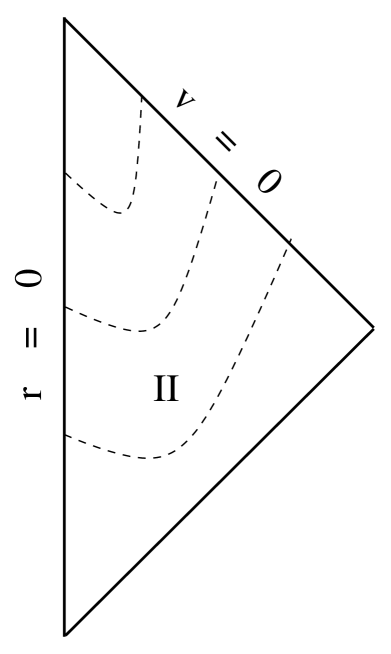
FIG. 7.: The Penrose diagram for the solutions given by Eqs.(101). The dashed lines represent the hypersurfaces $\phi(u,v)=$ const., the normal vector of which is always timelike. The whole spacetime is free of singularity except for the point ($u,v)=(0,0$).

However, applying Eq.(85) to the above solutions, we can consider the solutions in Region II, but which are now causally disconnected from Region I. These solutions are given by

$$e^{2\sigma(u,v)} = \frac{1}{(16\alpha^{2})^{\chi}}\,\frac{\left[\alpha(-u)^{1/2}+(-v)^{1/2}\right]^{4\chi}}{(uv)^{\chi}},$$ (97)

$$r(u,v) = \alpha^{2}(-u)+v,$$ (98)

$$\phi(u,v) = 2c\ln\left|\alpha(-u)^{1/2}+(-v)^{1/2}\right|+\phi^{1}_{0},\;\;\;\;(u,\;v\leq 0).$$ (99)

From these expressions, we find that

$$\theta_{l}=-\alpha^{-2}\,\theta_{n}=\frac{e^{-2\sigma}}{r},$$ (100)

which is non-negative; that is, the outgoing null geodesics are now no longer trapped. One can show that the null hypersurface $v=0$ is also future null infinity of Region II. Thus, the spacetime is geodesically maximal in this region. As a result, we also have

$$R=8\pi G\nabla_{a}\phi\nabla^{a}\phi=-2\alpha\chi(16\alpha^{2})^{\chi}\,\frac{(uv)^{\chi-1/2}}{\left|(-v)^{1/2}+\alpha(-u)^{1/2}\right|^{2(2\chi+1)}},$$ (101)

which shows that, when $\alpha<0$ the spacetime in this region is singular at $r=0$, and when $\alpha>0$ the spacetime is free of such singularities. Moreover, from Eq.(101) we can also see that the normal vector to the hypersurfaces $\phi(u,v)=$ const. is always timelike when $\alpha>0$, and quite similar to those given by Fig. 6. Thus, the solutions with $\alpha>0$ can be thought of as representing gravitational collapse starting from past null infinity at $u=-\infty$. Thus, we will only consider solutions with $\alpha>0$ for the current case of $\chi\geq 1$. As a result, the spacetime is free of singularities at the beginning of the collapse, but with a spacetime singularity forming at the point $(u,\,v)=(0,\,0)$. The corresponding Penrose diagram is given in Fig. 7. It is interesting to note that in this case, although no event horizon is formed, the spacetime singularity at the point $(u,v)=(0,0)$ is not naked and the only observers who are able to see the singularity there are those observers who arrive at that point.

It can be shown that in this case (with $\alpha>0$) the metric and the massless scalar field in Region II can be also written in the same form as that given by Eqs.(89) and (91).

In fact, from Eqs.(65–67) and Eqs.(89–91), we find that in the case $a_{0}b_{0}\not=0$, all the solutions that represent gravitational collapse of the massless scalar field can be cast in the form of Eqs.(89) and (91) in Region II. For that reason, when we consider linear perturbations in the next section, we will always refer to Eqs.(89) and (91) with $\chi\geq 1/2$ when considering the case of $a_{0}b_{0}\not=0$. In addition, because it is only the absolute value of $\alpha$ which enters these equations, we will from now on and without loss of generality assume that $\alpha>0$.

IV Linear Perturbations of the Self-Similar Solutions

We now turn to a study of the linear perturbations of the self-similar solutions presented in the last section. Let us consider perturbations given by

$$\sigma(z,\tau) = \sigma_{0}(z)+\epsilon\,\sigma_{1}(z)e^{k\tau},$$ (102)

$$s(z,\tau) = s_{0}(z)+\epsilon\,s_{1}(z)e^{k\tau},$$ (103)

$$\varphi(z,\tau) = \varphi_{0}(z)+\epsilon\,\varphi_{1}(z)e^{k\tau},$$ (104)

where $\epsilon$ is a very small real constant, and quantities with subscripts “1” denote perturbations, and those with “0” denote the self-similar solutions, given, respectively, by Eq.(38) with $s_{0}=z,\;\sigma^{1}_{0}=0$, Eq.(43) with $s_{0}=1,\;\sigma^{1}_{0}=0$, and Eqs.(89) and (91) with $\chi\geq 1/2$. It is understood that there may be many perturbation modes for different values (possibly complex) of the constant $k$. The general perturbation will be the sum of these individual modes. Those modes with $Re(k)>0$ grow as $\tau\rightarrow\infty$ and are referred to as unstable modes, while the ones with $Re(k)<0$ decay and are referred to as stable modes. By definition, critical solutions will have one and only one unstable mode. It should be noted that in writing Eq.(102), we have already used some of the gauge freedom available to us to write the perturbations such that they preserve the form of the metric (5). However, this does not completely fix the gauge freedom and we will return to this issue when we consider gauge modes.

To first order in $\epsilon$, it can be shown that the non-vanishing components of the Ricci tensor are given by

$$R_{uu} = -\frac{1}{r}\left(r_{,uu}-2\sigma_{,u}r_{,u}\right)$$ (105)

$$= -\frac{e^{2\tau}}{u^{2}_{0}s_{0}}\left[z^{2}s^{\prime\prime}_{0}-2z\sigma^{\prime}_{0}\left(zs^{\prime}_{0}-s_{0}\right)\right]$$ (109)

$$\quad-\epsilon\,\frac{e^{(2+k)\tau}}{u^{2}_{0}s_{0}}\Bigg{\{}z^{2}s^{\prime\prime}_{1}+2z(k-z\sigma^{\prime}_{0})s^{\prime}_{1}$$

$$\qquad\qquad\qquad-\left[z^{2}s^{-1}_{0}\left(s^{\prime\prime}_{0}-2\sigma^{\prime}_{0}s^{\prime}_{0}\right)+k(2z\sigma^{\prime}_{0}+1-k)\right]\,s_{1}$$

$$\qquad\qquad\qquad-2(zs^{\prime}_{0}-s_{0})(z\sigma^{\prime}_{1}+k\sigma_{1})\;\Bigg{\}}$$

$$R_{vv} = -\frac{1}{r}\left(r_{,vv}-2\sigma_{,v}r_{,v}\right)$$ (110)

$$= -\frac{e^{2\tau}}{u^{2}_{0}s_{0}}\left(s^{\prime\prime}_{0}-2\sigma^{\prime}_{0}s^{\prime}_{0}\right)$$ (112)

$$\quad-\epsilon\,\frac{e^{(2+k)\tau}}{u^{2}_{0}s_{0}}\Bigg{\{}s^{\prime\prime}_{1}-2\sigma^{\prime}_{0}s^{\prime}_{1}-s^{-1}_{0}\left(s^{\prime\prime}_{0}-2\sigma^{\prime}_{0}s^{\prime}_{0}\right)\,s_{1}-2s^{\prime}_{0}\sigma^{\prime}_{1}\Bigg{\}}$$

$$R_{uv} = -\frac{1}{r}\left(r_{,uv}+2r\sigma_{,uv}\right)$$ (113)

$$= -\frac{e^{2\tau}}{u^{2}_{0}s_{0}}\Big{[}zs^{\prime\prime}_{0}+2s_{0}\left(z\sigma^{\prime\prime}_{0}+\sigma^{\prime}_{0}\right)\Big{]}$$ (115)

$$\quad-\epsilon\,\frac{e^{(2+k)\tau}}{u^{2}_{0}s_{0}}\Bigg{\{}zs^{\prime\prime}_{1}+2zs_{0}\sigma^{\prime\prime}_{1}+ks^{\prime}_{1}+2(1+k)s_{0}\sigma^{\prime}_{1}-zs^{-1}_{0}s^{\prime\prime}_{0}s_{1}\Bigg{\}}$$

$$R_{\theta\theta} = 2e^{-2\sigma}rr_{,uv}$$ (116)

$$= 2zs_{0}s^{\prime\prime}_{0}e^{-2\sigma_{0}}$$ (118)

$$\quad+\epsilon\,2e^{k\tau-2\sigma_{0}}s_{0}\bigg{\{}zs^{\prime\prime}_{1}+ks^{\prime}_{1}+zs^{\prime\prime}_{0}\left(s^{-1}_{0}s_{1}-2\sigma_{1}\right)\bigg{\}}.$$

To zeroth order the Einstein field equations are given by Eqs.(19–23), while to first order they take the form

$$z^{2}s^{\prime\prime}_{1}+2z(k-z\sigma^{\prime}_{0})s^{\prime}_{1}\qquad\qquad\qquad\qquad\qquad\qquad$$ (119)

$$-\left[z^{2}s^{-1}_{0}\left(s^{\prime\prime}_{0}-2\sigma^{\prime}_{0}s^{\prime}_{0}\right)+k(2z\sigma^{\prime}_{0}+1-k)\right]\,s_{1}$$ (120)

$$-\,2(zs^{\prime}_{0}-s_{0})(z\sigma^{\prime}_{1}+k\sigma_{1})\qquad\qquad\qquad\qquad = -16\pi Gs_{0}\left(z\varphi^{\prime}_{0}-c\right)\left(z\varphi^{\prime}_{1}+k\varphi_{1}\right)$$ (121)

$$s^{\prime\prime}_{1}-2\sigma^{\prime}_{0}s^{\prime}_{1}-s^{-1}_{0}\left(s^{\prime\prime}_{0}-2\sigma^{\prime}_{0}s^{\prime}_{0}\right)\,s_{1}-2s^{\prime}_{0}\sigma^{\prime}_{1} = -16\pi Gs_{0}\varphi^{\prime}_{0}\varphi^{\prime}_{1}$$ (122)

$$zs^{\prime\prime}_{1}+2zs_{0}\sigma^{\prime\prime}_{1}+ks^{\prime}_{1}\qquad\qquad\qquad$$ (123)

$$+\,2(1+k)s_{0}\sigma^{\prime}_{1}-zs^{-1}_{0}s^{\prime\prime}_{0}s_{1} = -8\pi Gs_{0}\left[\left(2z\varphi^{\prime}_{0}-c\right)\varphi^{\prime}_{1}+k\varphi^{\prime}_{0}\varphi_{1}\right]$$ (124)

$$zs^{\prime\prime}_{1}+ks^{\prime}_{1}+zs^{\prime\prime}_{0}\left(s^{-1}_{0}s_{1}-2\sigma_{1}\right) = 0.$$ (125)

To zeroth order, the equation for the massless scalar field is given by Eq.(25) while, to first order, the scalar field equation is found to be

$$2zs_{0}\varphi^{\prime\prime}_{1}+\left[2zs^{\prime}_{0}+(1+2k)s_{0}\right]\,\varphi^{\prime}_{1}+ks^{\prime}_{0}\varphi_{1}\qquad\qquad$$ (126)

$$+\left(2z\varphi^{\prime}_{0}-c\right)s^{\prime}_{1}+\left[2z\varphi^{\prime\prime}_{0}+(1+k)\varphi^{\prime}_{0}\right]\,s_{1} = 0.$$ (127)

In order to be somewhat systematic in our examination of the perturbation equations, we will consider separately the same three cases that we did in section III, namely $a_{0}\not=0,\;b_{0}=0;\;a_{0}=0,\;b_{0}\not=0$ and $a_{0}b_{0}\not=0$. The notation will of necessity become rather complicated and we ask for the reader’s indulgence. For our part, we will try to keep the complexity under control and the physical interpretation near the fore.

A $a_{0}\not=0$ and $b_{0}=0$

In this case, the self-similar background solutions are given by Eq.(38) with $s_{0}(z)=z$ and $\sigma^{1}_{0}=0$. Substituting these solutions into Eqs.(119–126) we find

$$zs^{\prime\prime}_{1}+ks^{\prime}_{1} = 0$$ (128)

$$(k-\chi)\left[zs^{\prime}_{1}+(k-1)s_{1}\right] = 0$$ (129)

$$z(k+\chi)s^{\prime}_{1}-\chi s_{1}+2z^{2}\sigma^{\prime}_{1} = 16\pi cG\,z^{2}\varphi^{\prime}_{1}$$ (130)

$$z^{2}\sigma^{\prime\prime}_{1}+(1+k)z\sigma^{\prime}_{1} = -4\pi cG\,(k\varphi_{1}+z\varphi^{\prime}_{1})$$ (131)

$$2z^{2}\varphi^{\prime\prime}_{1}+(3+2k)z\varphi^{\prime}_{1}+k\varphi_{1} = -\frac{c}{z}\left[zs^{\prime}_{1}+(k-1)s_{1}\right].$$ (132)

It should be noted that in writing Eqs.(129–132), we have used Eq.(128). As usual, Eqs.(129) and (130) are constraints, and Eqs.(128), (131) and (132) are the dynamical equations. Due to the redundancy in the Einstein equations, these are not all independent and, e.g. it can be shown that Eq.(131) can be written in terms of the others.

Once these equations are integrated, one needs boundary conditions to complete the solution. Such boundary conditions are crucial for a proper determination of the eigenmodes but are rather subtle in general relativity. Indeed, there is no fixed prescription to follow [7, 12]. In the present case, the background spacetime has four boundaries, $u=\pm\infty$ and $v=0,\;\infty$. However, since the perturbation equations are of second order, it is usually sufficient to impose boundary conditions on only two hypersurfaces. As $\sigma_{1},\;s_{1}$ and $\varphi_{1}$ are functions of $z$ only, it is rather natural to choose the hypersurface $z=z_{0}$ as one of the two boundaries, that is, we assume that the perturbations are turned on at $z=z_{0}$, where $z_{0}$ is an arbitrary constant. Prior to $z=z_{0}$ the perturbations are zero. In order to match the perturbations smoothly across this surface, we require that $s_{1}(z_{0})=0=\varphi_{1}(z_{0})$. Also, by using the coordinate tranformations (6) we can always set $\sigma_{1}(z_{0})=0$. Then, on the hypersurface $z=z_{0}$ we have the boundary conditions,

$$\sigma_{1}(z_{0})=s_{1}(z_{0})=\varphi_{1}(z_{0})=0.$$ (133)

The second boundary has to be one of the two hypersurfaces, $v=0$ and $u=\infty$. As shown in the last section, the hypersurface $v=0$ is always singular in the present case and we do not know how to impose boundary conditions on such a surface. Therefore, in the following we shall choose the hypersurface $u=\infty$ as the second boundary. Because this surface represents future null infinity for this spacetime, it is reasonable to assume that the perturbations grow slower than the background. In the present case, we have $s_{0}(z)\sim z,\;\sigma_{0}(z)\sim\ln(z),\;\varphi_{0}(z)\sim\ln(z)$. However, considering the fact that $e^{\tau}\sim(-u)^{-1}$, we might require that, as $u\rightarrow\infty$, $\delta r(u,v)\equiv\epsilon(-u)s_{1}(z)e^{k\tau}$ and $\delta\varphi(u,v)\equiv\epsilon\varphi_{1}(z)e^{k\tau}$ be finite while $\delta\sigma(u,v)\equiv\epsilon\sigma_{1}(z)e^{k\tau}$ is requied to grow slower than $\ln(-u)$, as $u\rightarrow\infty$. Instead, we will choose to impose somewhat stronger conditions here, namely

$$\delta r(u,v),\;\;\delta\varphi(u,v),\;\;\delta\sigma(u,v)\rightarrow\;\;{\rm{finite}},$$ (134)

as $u\rightarrow\infty$. Clearly, if we find unstable modes with this stricter criterion of regularity, then in general the solutions will still be unstable.

Before proceeding to the full perturbation analysis, we need to address questions concerning gauge modes. Under the coordinate transformations

$$u\rightarrow u+\epsilon\xi_{1}(u),\;\;\;\;v\rightarrow v+\epsilon\xi_{2}(v),$$ (135)

we generate perturbations of the form

$$\delta\sigma = \frac{\epsilon}{2}\left\{\chi\left[\frac{\xi_{2}(v)}{v}-\frac{\xi_{1}(u)}{u}\right]+\xi^{\prime}_{1}(u)+\xi^{\prime}_{2}(v)\right\}$$ (136)

$$\delta r = \epsilon\xi_{2}(v)$$ (137)

$$\delta\varphi = \epsilon c\left(\frac{\xi_{2}(v)}{v}-\frac{\xi_{1}(u)}{u}\right),$$ (138)

where $\xi_{1}(u)$ and $\xi_{2}(v)$ are arbitrary functions. For such perturbations to take the forms of Eq.(102), we must choose

$$\xi_{1}(u)=\frac{c_{1}}{c}{u_{0}}^{k}(-u)^{1-k},\;\;\;\;\xi_{2}(v)=c_{2}{u_{0}}^{k}v^{1-k}$$ (139)

where $c_{1}$ and $c_{2}$ are arbitrary constants. Then, the solutions to the perturbation equations due to the gauge transformations are given by

$$s_{1}(z) = c_{2}z^{1-k}$$ (140)

$$\sigma_{1}(z) = \frac{c_{2}}{2}\,(1-k+\chi)z^{-k}-\frac{c_{1}}{2c}(1-k-\chi)$$ (141)

$$\varphi_{1}(z) = c_{1}+cc_{2}\,z^{-k}.$$ (142)

It can now be seen that our boundary conditions, Eqs.(133) and (134) eliminate each of these gauge modes.

Now let us turn to solving the perturbation equations given by Eqs.(128–132). From Eq.(129) we can see that there are two subcases which we need to consider separately, $k=\chi$ and $k\not=\chi$.

1 $k=\chi$

In this subcase, we have

$$k=\chi\equiv 8\pi Gc^{2}>0,$$ (143)

that is, the constant $k$ is real and strictly positive. Integrating Eq.(128) we obtain

$$s_{1}(z)=\cases{\beta\ln|z|+s^{0}_{1},&$k=\chi=1$,\cr\beta z^{1-\chi}+s^{0}_{1},&$k=\chi\not=1$,\cr}$$ (144)

where $\beta$ and $s^{0}_{1}$ are real integration constants.

Case (a) $\;k=\chi=1$: From Eqs.(128–132) we find that the solutions to the perturbation equations can be written

$$s_{1}(z) = \beta\ln|z|+s^{0}_{1}$$ (145)

$$\sigma_{1}(z) = 8\pi cG\,\varphi_{1}(z)+{\beta-s^{0}_{1}\over 2z}-\frac{\beta}{2z}\,\ln|z|+\sigma^{0}_{1}$$ (146)

$$\varphi_{1}(z) = c_{1}z^{-1/2}+c_{2}z^{-1}+\frac{c\beta}{z}\ln|z|$$ (147)

where $c_{1}$, $c_{2}$ and $\sigma^{0}_{1}$ are additional real, integration constants. Applying the boundary conditions at $z=z_{0}$, Eq.(133), to these solutions, we find that

$$s^{0}_{1} = -\beta\ln z_{0}$$ (148)

$$\sigma^{0}_{1} = -\frac{\beta}{2z_{0}}$$ (149)

$$c_{1} = -z_{0}^{-1/2}\left[c_{2}+c\beta\ln(z_{0})\right],$$ (150)

from which we obtain

$$r(u,v) = (-u)\left[s_{0}(z)+\epsilon s_{1}(z)e^{k\tau}\right]$$ (151)

$$= v+\epsilon\beta u_{0}\ln\left(\frac{v}{-z_{0}u}\right).$$ (152)

From this form for $r(u,v)$, we can see that the condition of finiteness as $u\rightarrow\infty$, Eq.(134), leads to $\beta=0$. Setting $\beta=0$ in these solutions yields that $\delta\sigma$ and $\delta\varphi$ are all finite as $u\rightarrow\infty$. Therefore, in this case ($k=\chi$), there is a perturbation mode with $k=1$ which satisfies the appropriate boundary conditions, Eqs.(133) and (134). Of course, because $k>0$, this is an unstable mode.

Case (b) $\;k=\chi\not=1$: In this case, the perturbation equations given by Eqs.(128–132) can again be integrated to yield

$$s_{1}(z) = \beta z^{1-\chi}+s^{0}_{1}$$ (153)

$$\sigma_{1}(z) = 8\pi cG\,\varphi_{1}(z)-\frac{\beta}{2}(2\chi-1)\,z^{-\chi}-\frac{s^{0}_{1}\,\chi}{2}\,z^{-1}+\sigma^{0}_{1}$$ (154)

$$\varphi_{1}(z) = \cases{c_{1}z^{-1/2}+c_{2}z^{-\chi}+c\,s^{0}_{1}\,z^{-1},&$k\neq 1/2$ ,\cr c_{1}z^{-1/2}+c_{2}z^{-1/2}\,\ln|z|+c\,s^{0}_{1}\,z^{-1},&$k=1/2$ .\cr}$$ (155)

On application of the boundary conditions, Eqs. (133) and (134), at $z=z_{0}$ and $u\rightarrow\infty$, it can be shown that there are nontrivial perturbations for $k>1/2$ while for $k\leq 1/2$, no solutions exist which are compatible with the boundary conditions.

We conclude this section by noting that all the solutions given by Eq.(38) of section IIIA with $\chi>1/2$ have an unstable mode with $k=\chi$.

2 $k\not=\chi$

In this subcase, the constant $k$ can be complex, and from Eqs.(128–132) we find that we can again integrate the perturbation equations yielding

$$s_{1}(z) = \beta z^{1-k}$$ (156)

$$\sigma_{1}(z) = 8\pi cG\varphi_{1}(z)+\frac{1}{2}\beta(1-k-\chi)z^{-k}+\sigma^{0}_{1}$$ (157)

$$\varphi_{1}(z) = \cases{c_{1}z^{-1/2}+c_{2}z^{-k},&$k\neq 1/2$\cr c_{1}z^{-1/2}+c_{2}z^{-1/2}\,\ln|x|,&$k=1/2$ ,\cr}$$ (158)

where $\beta$, $\sigma^{0}_{1}$, $c_{1}$, and $c_{2}$ are additional arbitrary (but now possibly complex) constants of integration. It is interesting to note that setting $c_{1}=0=s^{0}_{1}$ and $c_{2}=c\beta$ the above perturbations will reproduce the gauge modes given by Eq.(140) that do not satisfy the boundary conditions (133) and (134). However, the general perturbations represented by Eqs.(158) will satisfy these conditions, provided that

$$\beta=\sigma^{0}_{1} = 0$$ (159)

$$c_{1} = -c_{2}\,z_{0}^{(1-2k)/2}$$ (160)

$$Re(k) > \frac{1}{2},\;\;\;\;\;(k\not=\chi).$$ (161)

Because $Re(k)>1/2>0$ for any given $\chi$, we can see that the solutions given by Eq.(38) are unstable with an infinite number of unstable modes. This result is consistent with King’s conjecture [13], namely: Non-scalar singularities are unstable to perturbations and will eventually give rise to scalar singularities.

B $a_{0}=0$ and $b_{0}\not=0$

In this case, the self-similar background solutions are given by Eq.(43) with $s_{0}=1,\;\sigma^{1}_{0}=0$. Substituting these solutions into Eqs.(119–126) we find that

$$z^{2}s^{\prime\prime}_{1}+(2k+\chi)zs^{\prime}_{1}-k(1-k-\chi)s_{1}\qquad$$ (162)

$$+\,2(k\sigma_{1}+z\sigma^{\prime}_{1}) = 16\pi cG(k\varphi_{1}+z\varphi^{\prime}_{1}),$$ (163)

$$z\sigma^{\prime\prime}_{1}+(1+k)\sigma^{\prime}_{1} = 4\pi cG\varphi^{\prime}_{1},$$ (164)

$$zs^{\prime\prime}_{1}+\chi s^{\prime}_{1} = 0,$$ (165)

$$zs^{\prime\prime}_{1}+ks^{\prime}_{1} = 0,$$ (166)

$$2z\varphi^{\prime\prime}_{1}+(1+2k)\varphi^{\prime}_{1} = cs^{\prime}_{1}.$$ (167)

Note that in writing the above equations, we have used Eqs.(165) and (166) to simplify the expressions somewhat.

Following arguments similar to those given in the previous subsection for ingoing solutions with $a_{0}\not=0$ and $b_{0}=0$, we here impose boundary conditions on the hypersurfaces $z=z_{0}$ and $v=\infty$. The conditions on the hypersurface $z=z_{0}$ are the same as those given by Eq.(133). On the hypersurface, $v=\infty\;(z=\infty)$, we take as our condition that the perturbations should grow more slowly than the unperturbed, background solution. At future null infinity these conditions become

$$s_{1}(z),\;\;\varphi_{1}(z)\rightarrow\;\;{\rm finite},$$ (168)

$$\sigma_{1}(z)\;\;{\rm grows}\;\;{\rm slower}\;\;{\rm than}\;\;\ln z,$$ (169)

as $z\rightarrow\infty$. As a result, it can be shown that the gauge modes of Eqs.(136–139) are given, in the current case, by

$$\sigma_{1}(z)=c_{0}z^{-k}+c_{1},\;\;\;\;\;s_{1}(z)=\varphi_{1}(z)=0.$$ (170)

Returning to the perturbation equations in Eqs.(162–167), we can see from these that there are two distinct possibilities, $s^{\prime}_{1}(z)\not=0$ and $s^{\prime}_{1}(z)=0$. In the former case it can be shown that the above equations have no solution consistent with the above boundary conditions at $z=z_{0}$ and $v\rightarrow\infty$. Thus, in the following we need only consider the case $s^{\prime}_{1}(z)=0$. In this latter case, the perturbation equations can be rewritten as

$$s_{1}(z)=s^{0}_{1},$$ (171)

$$z\sigma^{\prime}_{1}+k\sigma_{1}=8\pi cG(k\varphi_{1}+z\varphi^{\prime}_{1})+\frac{1}{2}s^{0}_{1}k(1-k-\chi),$$ (172)

$$2z\varphi^{\prime\prime}_{1}+(1+2k)\varphi^{\prime}_{1}=0.$$ (173)

The general solution to these equations is then

$$s_{1}(z) = s^{0}_{1}$$ (174)

$$\sigma_{1}(z) = 8\pi cG\,\varphi_{1}(z)+\sigma^{0}_{1}\,z^{-k}+\frac{s^{0}_{1}}{2}(1-k-\chi)$$ (175)

$$\varphi_{1}(z) = \cases{\beta\ln z+\varphi^{0}_{1},&$k=\frac{1}{2}$,\cr\beta z^{(1-2k)/2}+\varphi^{0}_{1},&$k\neq\frac{1}{2}$,\cr}$$ (176)

where $\beta$, $\varphi_{1}^{0}$ and $\sigma^{0}_{1}$ are integration constants (real for $k=1/2$ and possibly complex otherwise).

Note that the gauge modes of Eq.(170) can be obtained from Eqs.(174) by setting $\sigma_{1}^{0}=c_{0}$ and $s_{1}^{0}=\beta=0$. However, these gauge modes are completely eliminated by our boundary conditions (133) and (168).

Applying the boundary conditions to the general perturbation solutions given by Eqs.(174) eliminates all the perturbations for $k=1/2$ while for $k\not=1/2$ there are nontrivial perturbations which do satisfy the boundary conditions provided we have

$$s^{0}_{1}=\sigma_{1}^{0} = 0$$ (177)

$$\varphi^{0}_{1} = -\beta z_{0}^{(1-2k)/2}$$ (178)

$$Re(k) > \frac{1}{2}.$$ (179)

Because the nontrivial perturbations in this case have $Re(k)>1/2>0$, we can see that all the solutions in section IIIB given by Eq.(43) are unstable with an infinite number of unstable modes.

C $a_{0}b_{0}\not=0$

With this most general case, we can interpret the solution as collapsing and might hope that by examining the perturbative structure, we can determine if there are critical solutions. The self-similar background solutions are given by Eqs.(89) and (91) with $\chi\geq 1/2$. Substituting these solutions into Eq.(125) we find that

$$zs^{\prime\prime}_{1}+ks^{\prime}_{1}=0,$$ (180)

which has the general solution

$$s_{1}(z)=\cases{\beta\ln z+s^{0}_{1},&$k=1$,\cr\beta z^{1-k}+s^{0}_{1},&$k\not=1$,\cr}$$ (181)

where $\beta$ and $s^{0}_{1}$ are the integration constants.

Before solving the rest of the differential equations, (119–123) and (126), let us again first consider the boundary conditions. As we can see from Figs. 5 and 7, Region II of the spactime has only three boundaries: the center of the spacetime at $z=\alpha^{2}$, the event horizon at $z=0$, and past null infinity at $u=-\infty$. In this paper we choose $z=\alpha^{2}$ and $z=0$ as the surfaces on which boundary conditions will be imposed.

To see what kind of boundary conditions should be imposed at each of these surfaces, first notice that $z=\alpha^{2}$ is the center of the background. It is therefore natual to assume that this will remain true even after the spacetime is perturbed, that is, $s_{1}(z=\alpha^{2})=0$. In addition, because the background is free of spacetime singularities at the origin in Region II, the perturbed spacetime should remain regular there as well. It can be shown that this will only be the case if $\sigma_{1}(z)$ and the quantity $\left[(\alpha^{2}-z)\varphi^{\prime}_{1}-2k\varphi_{1}\right]$ remain finite. Summarizing the above, we impose the following boundary conditions at the origin of coordinates

$$s_{1}(y)\,\Big{|}_{y=1} = 0$$ (182)

$$\sigma_{1}(y)\,\Big{|}_{y=1} \sim \;{\rm finite}$$ (183)

$$\left\{(1-y)\frac{d\varphi_{1}(y)}{dy}-2k\varphi_{1}(y)\right\}\,\Bigg{|}_{y=1} \sim \;{\rm finite},$$ (184)

where we have defined the new variable $y\equiv z/\alpha^{2}$ such that $z=\alpha^{2}$ corresponds to $y=1$.

The other boundary at $z=0$, or $v=0$, represents the event horizon. We would like to be able to assume that no matter comes out of Region I into Region II. Naively, we can express this as

$$\phi_{,v}=0$$ (185)

as $v\rightarrow 0^{-}$. However, it can be shown that this condition does not hold even for the background solutions. Indeed, as $v\rightarrow 0$, we have

$$\frac{\partial\phi_{0}(u,v)}{\partial v}=\frac{c}{(-uv)^{1/2}\alpha(1+y^{1/2})}\rightarrow\infty.$$ (186)

But this is nothing more than the statement that in the coordinates $u$ and $v$, the metric coefficients are singular there. Having found the analytic extension of these collapsing solutions across the hypersurface $v=0$ in the coodinates $\bar{u}$ and $\bar{v}$, we should understand the no outflow condition, Eq.(185), in terms of $\bar{v}$ rather than the “bad” coordinate $v$. This argument is further justified by noting that for the unperturbed, background solution, we have $\phi_{0,\bar{v}}\rightarrow 0$, as $\bar{v}\rightarrow 0$. In terms of our rescaled self-similar variable $y$, it can be shown that this condition is equivalent to $y^{\chi}\varphi^{\prime}_{1}(y)\rightarrow 0$. This then, becomes our boundary condition on $\varphi(y)$ at $y=0$.

For the boundary conditions on the other fields at $y=0$, recall that when we extended the background solutions from Region I to Region II, we required that the extension be analytic. Otherwise, the extension will not be unique and in some cases may even be meaningless. To have consistency between the unperturbed and perturbed spacetimes, we will assume that the perturbations are also analytic across $y=0$. Given this, we find that the boundary conditions at the event horizon $y=0$ become

$$s_{1}(y),\;\ \sigma_{1}(y),\;\varphi_{1}(y)\;\;{\rm are}\;{\rm analytic},$$ (187)

$$y^{\chi}\frac{d\varphi_{1}(y)}{dy}\rightarrow 0.$$ (188)

Again, a word about gauge modes is in order. It can be shown that in the present case the gauge transformations (135) lead to the perturbations

$$s_{1}(y) = \beta\left(\alpha^{2}y\right)^{1-k}+s^{0}_{1}$$ (189)

$$\varphi_{1}(y) = -\frac{c\beta}{\alpha^{2k}(1+y^{1/2})}\left(y^{1/2-k}-\beta^{-1}\alpha^{2(k-1)}s^{0}_{1}\right)$$ (190)

$$\sigma_{1}(z) = \frac{1}{2(1+y^{1/2})}\Bigg{\{}\,\chi\left(1-y^{1/2}\right)\left(\frac{s^{0}_{1}}{\alpha^{2}}+\frac{\beta}{\alpha^{2k}}y^{-k}\right)$$ (192)

$$\qquad\qquad\qquad+\,(1-k)\left(1+y^{1/2}\right)\left(\frac{s^{0}_{1}}{\alpha^{2}}-\frac{\beta}{\alpha^{2k}}y^{-k}\right)\Bigg{\}}.$$

Let us now consider the remaining perturbation equations given by Eqs.(119–123) and (126). It turns out to be convenient to consider the two cases $k=1$ and $k\not=1$ separately.

1 $k=1$

In this case from Eq.(181) we find that

$$s_{1}(y)=\beta\ln\left(y\right).$$ (193)

where, in writing the above expression, we have chosen $s^{0}_{1}=-2\beta\ln(\alpha)$ so that the boundary condition $s_{1}(y=1)=0$ is satisfied. Inserting Eq.(193) into Eqs.(119–123) and (126), we find that only two of the four equations are independent

$$\sigma_{1}(y) = 8\pi cG\left(1-y^{1/2}\right)\left[y^{1/2}\left(1+y^{1/2}\right)\frac{d\varphi_{1}(y)}{dy}+\varphi_{1}\right]$$ (196)

$$-\frac{\beta}{2\alpha^{2}y(1+y^{1/2})^{2}}\Bigg{[}\,(1-\chi)(1+y^{2})$$

$$\qquad\qquad\qquad\qquad+\,2(1+\chi)y+2y^{1/2}(1+y)\Bigg{]}$$

$$y(1-y)\frac{d^{2}\varphi_{1}}{dy^{2}} + \left[\lambda-(a+b+1)y\right]\frac{d\varphi_{1}}{dy}-ab\varphi_{1}=f(y),$$ (197)

where

$$a = 1,\;\;\;b=\frac{1}{2},\;\;\;\lambda=\frac{3}{2},$$ (198)

$$f(y) \equiv \frac{c\beta}{2\alpha^{2}y(1+y^{1/2})^{2}}\left[(1-y)-y^{1/2}\ln(y)\right].$$ (199)

Eq.(197) is the inhomogeneous hypergeometric equation [14], and the corresponding general solution is given by

$$\varphi_{1}(y)=\varphi_{1}^{h}(y)+\varphi_{1}^{s}(y),$$ (200)

where $\varphi_{1}^{s}(y)$ is a particular solution of the inhomogeneous equation (197), and $\varphi_{1}^{h}(y)$ is the general solution of the associated homogeneous equation,

$$y(1-y)\frac{d^{2}\varphi_{1}}{dy^{2}}+\left[\lambda-(a+b+1)y\right]\frac{d\varphi_{1}}{dy}-ab\varphi_{1}=0.$$ (201)

The general solution $\varphi^{h}_{1}(y)$ can be written as a linear combination of two independent solutions $\varphi^{1}_{1}$ and $\varphi^{2}_{1}$

$$\varphi_{1}^{h}(y)=c_{1}\,\varphi^{1}_{1}(y)+c_{2}\,\varphi^{2}_{1}(y),$$ (202)

where $c_{1}$ and $c_{2}$ are two arbitrary constants, and $\varphi^{1}_{1}$ and $\varphi^{2}_{1}$ are given by

$$\varphi^{1}_{1} = 2F(1,\frac{1}{2};\frac{3}{2};y)=\frac{1}{y^{1/2}}\ln\left(\frac{1+y^{1/2}}{1-y^{1/2}}\right),$$ (203)

$$\varphi^{2}_{1} = y^{-1/2}F(\frac{1}{2},0;\frac{1}{2};y)=y^{-1/2},$$ (204)

with $F(a,b;\lambda;y)$ denoting the hypergeometric function. A particular solution of the inhomogeneous equation (197) can be found and is given by

$$\varphi^{s}_{1}(y) = \frac{c\beta}{\alpha^{2}(1+y^{1/2})}\left[\ln y-2\left(\frac{1+y^{1/2}}{y^{1/2}}\right)\ln\left(\frac{1+y^{1/2}}{2}\right)\right].$$ (205)

From Eqs.(198–205), we can show that as $y\rightarrow 1$, we have

$$\varphi_{1}(y)\approx\frac{1}{y^{1/2}}\left[c_{1}\ln\left(\frac{1+y^{1/2}}{1-y^{1/2}}\right)+c_{2}\right].$$ (206)

As a result, the boundary condition for $\varphi_{1}$ in Eq.(182) holds only if $c_{1}=0$ while the condition for $\sigma_{1}(y)$ at $y=1$ does not impose any additional restrictions.

With regard to the boundary conditions at $y=0$, we find from Eqs.(193) and (205) that the conditions on $s_{1}(y)$ and $\sigma_{1}(y)$ further demand $c_{2}=\beta=0$. Therefore, in the case that $k=1$, the boundary conditions (182) and (187) eliminate all the perturbations.

2 $k\not=1$

When $k\not=1$, we have

$$s_{1}(y)=c_{0}\alpha^{2}\left(y^{1-k}-1\right),$$ (207)

where $c_{0}\equiv\alpha^{-2k}\beta$. Note that now the constant $k$ can be complex, as can $c_{0}$. Substituting Eq.(207) into Eqs.(119–123) and (126), we find that now there are also only two independent equations, which can be written as

$$k\,\sigma_{1}(y) = \frac{\chi}{c}(1-y^{1/2})\left[y^{1/2}(1+y^{1/2})\frac{d\varphi_{1}(y)}{dy}+k\varphi_{1}\right]$$ (210)

$$-\,\frac{c_{0}(1-k)}{2(1+y^{1/2})}\bigg{[}\,\left(k+\chi\right)\left(1+y^{1/2-k}\right)$$

$$\qquad\qquad\qquad\qquad+\left(k-\chi\right)\left(y^{1/2}+y^{-k}\right)\bigg{]}$$

$$y(1-y)\frac{d^{2}\varphi_{1}}{dy^{2}} + \left[\lambda-(a+b+1)y\right]\frac{d\varphi_{1}}{dy}-ab\varphi_{1}=f(y),$$ (211)

but now with

$$a = k,\;\;\;\;b=\frac{1}{2},\;\;\;\;\lambda=k+\frac{1}{2},$$ (212)

$$f(y) \equiv \frac{c\beta}{2\alpha^{2k}y^{k+1/2}(1+y^{1/2})^{2}}\left[(1-k)(1-y^{k})y^{1/2}-ky(1-y^{k-1})\right].$$ (213)

Similar to the previous case, the general solution of Eq.(211) can be written in the same forms as those given by Eqs.(200–202), but $\varphi^{1}_{1}$ and $\varphi^{2}_{1}$ now are given by $\varphi^{1}_{1}=F(\frac{1}{2},k;k+\frac{1}{2};y)$, and $\varphi^{2}_{1}=F(\frac{1}{2},k;1;1-y)$. In addition, it can be shown that a particular solution of the inhomogenuous equation (211) is given by

$$\varphi^{s}_{1}(y)=-\frac{c\beta}{\alpha^{2k}}\,\frac{1+y^{1/2-k}}{1+y^{1/2}}.$$ (214)

Thus, the general solution for $\varphi_{1}(y)$ in the present case is given by

$$\varphi_{1}(y) = c_{1}\,F(\frac{1}{2},k;k+\frac{1}{2};y)+c_{2}\,F(\frac{1}{2},k;1;1-y)-\frac{c\beta}{\alpha^{2k}}\,\frac{1+y^{1/2-k}}{1+y^{1/2}}.$$ (215)

From Eqs.(207), (210) and (215) we can see that when $c_{1}=c_{2}=0$, the perturbations reduce to those given in Eq.(189) and which are purely gauge modes. Therefore, in the following we will restrict ourselves to those solutions for which $\left|c_{1}\right|^{2}+\left|c_{2}\right|^{2}\not=0$.

Considering first the boundary conditions at the origin, $y=1$, we note the following limiting relations as $y\rightarrow 1$

$$F(\frac{1}{2},k;k+\frac{1}{2};y) \rightarrow -\frac{1}{2}(2k-1)A(k)\ln(1-y)+A_{1}(y;k)$$ (216)

$$F(\frac{3}{2},k+1;k+\frac{3}{2};y) \rightarrow \frac{1}{2}(4k^{2}-1)A(k)\left(\frac{2}{k(1-y)}+\ln(1-y)\right)+A_{2}(y;k)$$ (217)

where $A(k)\equiv\Gamma(k-\frac{1}{2})/\left(\Gamma(k)\Gamma(\frac{1}{2})\right)$, and $A_{1}(y;k)$ and $A_{2}(y;k)$ are the finite pieces of the hypergeometric functions in the limit as $y\rightarrow 1$. Then, from Eqs.(215–216) and the relation

$$\frac{d}{dz}F(a,b;\lambda;z)=\frac{ab}{\lambda}F(a+1,b+1;\lambda+1;z),$$ (218)

we find that the boundary conditions given by Eq.(182) at $y=1$ will hold, provided that

$$c_{1}=0.$$ (219)

For the boundary conditions at $y=0$ as given in Eq.(187), we first recall that our imposition of analyticity on the extended spacetime exploited the barred coordinate system. Doin the same here, we notice that $y=\alpha^{-2}v/u=\alpha^{-2}(\bar{v}/\bar{u})^{2n}$ and

$$s_{1}(y)=c_{0}\alpha^{2}\left(\alpha^{-2}\left(\frac{\bar{v}}{\bar{u}}\right)^{2n(1-k)}-1\right).$$ (220)

Thus, to have $s_{1}(y)$ be analytic across the boundary $y=0$ (i.e. $\bar{v}=0$), we must have

$$k=\frac{m}{2n}<1,$$ (221)

where $m$ is a positive integer. Due to the properties of the hypergeometric functions, it is convenient to consider separately the cases $k=l+\frac{1}{2}$ and $k\not=l+\frac{1}{2}$, where $l$ is a non-negative integer.

Case (a) $\;k=l+\frac{1}{2}$: In this case, as $y\rightarrow 0$, we find that

$$F(\frac{1}{2},k;1;1-y) \rightarrow \frac{(l-1)!\,y^{-l}}{\Gamma(\frac{1}{2}+l)\Gamma(\frac{1}{2})}\,\sum^{l-1}_{p=0}{\frac{(a-l)_{p}(b-l)_{p}}{(1-l)_{p}\,p!}\,y^{p}}$$ (223)

$$-\frac{(-1)^{l}}{\Gamma(\frac{1}{2}-l)\Gamma(\frac{1}{2})}\,\ln y.$$

Inserting the above expression into Eq.(215) and considering Eq.(219), one quickly sees that the condition that $\varphi_{1}(y)$ be analytic across the hypersurface $y=0$ can only be true for $k<1/2$ and $c_{2}=0$. Because the boundary conditions as $y=0$ force us to take $c_{1}=c_{2}=0$, we can see that the corresponding perturbations are purely gauge. Thus, we need no longer consider the case of $k=l+\frac{1}{2}$.

Case (b) $\;k\not=l+\frac{1}{2}$: In this case, it can be shown that in the limit $y\rightarrow 0$

$$F(\frac{3}{2},k+1;2;1-y) \rightarrow k^{-1}A(k)\bigg{[}(2k-1)y^{-1/2-k}-(1-k)y^{1/2-k}\bigg{]}+A_{3}(y;k)$$ (224)

where $A_{3}(y;k)$ is again the finite portion of the hypergeometric portion in the limit as $y\rightarrow 0$. Inserting this into the general solution for $\varphi_{1}(y)$ as given in Eq.(215) together with the fact that we still have $c_{1}=0$, we can find the limiting behavior of the derivative of $phi_{1}(y)$ as $y\rightarrow 0$, namely

$$\frac{d\varphi_{1}(y)}{dy} \rightarrow \frac{1}{2}\Big{\{}\,cc_{0}\left[y^{-1/2}+2(1-k)y^{-k}\right]$$ (228)

$$\qquad\qquad+c_{2}(2k-1)A(k)y^{-1/2-k}$$

$$\qquad\qquad+\left[cc_{0}(10k-7)-c_{2}(1-k)A(k)\right]\,y^{1/2-k}\Big{\}}$$

$$\qquad\qquad+A_{4}(k)$$

where, again, $A_{4}(y;k)$ is the finite part. Now, one can see that the boundary condition of vanishing of $y^{\chi}\,\varphi^{\prime}_{1}(y)$ at $y=0$ can only be true if

$$k<\chi-\frac{1}{2}\;\;{\rm and}\;\;\chi>\frac{1}{2}$$ (229)

because we want to demand that $c_{2}\not=0$. Otherwise, the perturbations would again be purely gauge.

We are not yet done as we must still consider the effect of imposing analyticity on $\sigma_{1}(y)$ at $y=0$. From Eq.(224) and the asymptotic behavior of

$$F(\frac{1}{2},k;1;1-y)\rightarrow A(k)y^{1/2-k}+A_{5}(k),$$ (230)

as $y\rightarrow 0$, we get that

$$\sigma_{1}(y) \rightarrow \frac{\chi}{c}\left(A(k)c_{2}-cc_{0}\right)\,y^{1/2-k}+\frac{1}{2}\Big{[}A(k)\chi(2k-1)c_{2}-(1-\chi-k)c_{0}\Big{]}\,y^{-k}+\sigma_{1}^{0}$$ (231)

as $y\rightarrow 0$. Thus, to have $\sigma_{1}(y)$ be analytic across the hypersurface $y=0$, we must assume

$$k<\frac{1}{2}\;\;{\rm and}\;\;c_{2}=\frac{1-\chi-k}{\chi(2k-1)A(k)}c_{0}.$$ (232)

When $k=1-\chi$ (i.e. $m=1$), we can see from the above expression that $c_{2}=0$. In other words, the mode $m=1$ is a pure gauge mode. Thus, physically relevant perturbations will have $m\not=1$.

Combining Eqs. (80), (221) and (229) with Eq.(232), we find that in the present case all the perturbations with

$$c_{1}=0,\;\;\;c_{2}=\frac{n(1-m)\Gamma(k)\Gamma(\frac{1}{2})}{(m-n)(2n-1)\Gamma(k-\frac{1}{2})}c_{0},$$ (233)

$$k=\frac{m}{2n},\;\;\;1<m<n-1,\;\;\;\;\;n>1,$$ (234)

satisfy the boundary conditions (182) and (187).

Therefore, for any parameter $n>2$, the corresponding solution of Eqs.(89) and (91) has $(n-3)$ unstable modes. In particular, the one with $n=4$ only has one unstable mode. By definition this solution represents a critical solution [2]. This is consistent with Garfinkle’s original observations [7]. However, it is a departure from the perturbation analysis of [9] where they calculate the $n=2$ solution to have a single unstable mode. The discrepancy between that work and ours would seem to lie in the choice of boundary conditions for the perturbation problem. Though both works consider the same boundaries at the origin ($y=1$) and the horizon ($y=0$), we have the added condition that nothing escape from the horizon. This would seem to eliminate some of the additional modes found in [9].

V Critical Collapse of Scalar Field With Potential

In this section, following [10] we argue that the critical solution with $n=4$ (or $\chi=7/8$) for the massless scalar field collapse found in the last section is also the critical solution for the collapse of a scalar field with any potential $V(\phi)$ and cosmological constant $\Lambda$, provided that the condition (31) holds. As shown in section III, because of the presence of these terms, globally self-similar solutions do not exist, although in the limit $\tau\rightarrow\infty$ asymptotically self-similar solutions do exist. Fortunately for the study of critical collapse, this is sufficient. Indeed, initial configurations for collapsing gravitational systems can be quite different. This is the case even in situations where globally self-similar solutions are permitted. Thus, in generic cases the spacetime will become self-similar only after the passage of a sufficent amount of time during which the original differences will be washed away and the collapse approaches a self-similar evolution, such that the physics on large scales is related to that on small scales in a universal manner. A schematic illustration of this process is given in Fig. 8. Region $A$ represents a region where the influence of the terms $V(\phi)$ and $\Lambda$ in Einstein field equations is still very strong, and the corresponding spacetime is significantly different from that of the critical solution. In particular, no trapped surfaces have been formed so far. As $\tau$ grows, the differences are smoothed out, and when $\tau$ grows to a certain value, say, $\tau=\tau_{1}$, the differences become very small and can be considered as perturbations on top of the the self-similar critical solution. The region where such perturbations are valid is denoted as region $B$ in Fig. 8. Clearly, the time $\tau_{1}$ is dependent on the initial-data, and by fine tuning one can find out which initial data leads to critical collapse and which does not. When the strength of the initial data is larger than that required for critical collapse, the collapse will be strong enough to form black hole, while when weaker, the scalar field will reflect through the origin before a black hole can be formed and subsequently disperse entirely to infinity. In region $B$, the solutions to the whole problem can be expanded in the form [10],

$$A(\tau,z)=\sum^{\infty}_{n=0}{e^{-n\tau}A^{(n)}_{*}(z)},$$ (235)

where $A=(\sigma,\;s,\;\varphi)$, and $A^{(0)}_{*}$ denotes the critical solution. Substituting the above expression into the Einstein field equations (19–25), and then separating terms by powers of $e^{-\tau}$, we find that, to zeroth order, the resultant equations are exactly those given by Eqs.(32–36) for the self-similar critical solution $A^{(0)}_{*}$, which are independent of other higher terms. On the other hand, the equations for $A^{(n)}_{*}$’s with $n\geq 1$ are always coupled to its lower terms, $A^{(n-1)}_{*},\cdots,A^{(0)}_{*}$. This allows us to determine $A^{(n)}_{*}$ recursively starting with $A^{(0)}_{*}$. Thus, in principle once $A^{(0)}_{*}$ is known, we can find all the higher terms $A^{(n)}_{*}$. In particular, one can show that $A^{(1)}_{*}$ satisfies the same equations as those for $A_{1}(z)$ given by Eq.(119–126) with $k=-1$, where $A_{1}(z)=(s_{1},\;\sigma_{1},\;\varphi_{1})$. Following the analysis given there, we find that $A^{(1)}_{*}$ is well-behaved in region $B$, regular at $r=0$, and analytical across the hypersurface ${v}=0$. Since the higher order terms $A^{(n)}_{*}$ satisfy similar types of differential equations as those for $A^{(1)}_{*}$, and also these higher terms in (235) all correspond to stable modes ($k<0$) of perturbations given by Eq.(102), it is quite reasonable to expect that all the higher order terms in Eq.(235) are well behaved in Region $B$, and in the limit $\tau\rightarrow\infty$ Eq.(235) converges to $A^{(0)}_{*}$. Note that $A^{(0)}_{*}$ is well-behaved in the whole region $B$, except on the hypersurface ${v}=0$. However, this divergence is weak (logarithmically) and is due entirely to the choice of coordinates. As shown in section III, in terms of $\bar{u}$ and $\bar{v}$ the metric cofficients are well behaved there. In review of all the above, we can see that Eq.(235) indeed represents solutions to the full problem, that is, solutions of Einstein-scalar equations with potential $V(\phi)$ and the cosmological constant $\Lambda$.

FIG. 8.: Global structure of near-critical gravitational collapse. In region $A$ the effects of the terms $V(\phi)$ and $\Lambda$ are strong and the spacetime will, in general be very different from that of the critical solution. In particular, an apparent horizon will not have formed. With increasing time, however, the effects of the potential will become more and more weak such that, in region $B$ and for those initial configurations with initial data close to criticality, those effects can be considered as perturbations of the critical solution. In this region, supercritical configurations will form, in the end, black holes, while subcritical configurations will reflect through the origin and disperse to infinity without formating black holes. The line $AH$ represents the apparent horizon formed in the supercritical collapse.

Now let us consider the linear perturbations of the solutions (235), which can be written as

$$\delta A(\tau,z)=e^{k\tau}\delta_{k}A(\tau,z),$$ (236)

where $\delta_{k}A(\tau,z)$ denotes the general perturbations of $A(\tau,z)$ for the mode $k$, similar to that given by Eq.(102), but now depending on both of $\tau$ and $z$. However, we can expand it in a similar form as that given by Eq.(235),

$$\delta_{k}A(\tau,z)=\sum^{\infty}_{n=0}{e^{-n\tau}\delta_{k}A^{(n)}(z)}.$$ (237)

As $A(\tau,z)$ is completely determined by $A^{(0)}_{*}$, $\delta_{k}A(\tau,z)$ is totally specified by its leading term $\delta_{k}A^{(0)}(z)$. Indeed, substituting Eqs.(235–237) into the Einstein field equations (19–25), we find that $\delta_{k}A^{(0)}(z)$ satisfies the same differential equations (119–126) for $A_{1}(z)$, where the background depedence is only on terms of $A^{(0)}_{*}$. Consequently, the spectrum for the perturbations of $\delta_{k}A^{(0)}(z)$ is the same as that of $A_{1}(z)$. Once $\delta_{k}A^{(0)}(z)$ is known we can find the higher order terms $\delta_{k}A^{(n)}(z)$ recursively. In this way, we can see that the spectras of perturbations in the cases with or without $V(\phi)$ and $\Lambda$ will be exactly the same. In particular, the critical solution for the massless scalar field is also a critical solution for a scalar field with potential in a non-vanishing cosmological constant background (with the possibilities of being either negative or positive), provided Eq.(31) holds.

VI Conclusions

In this paper, we have considered the Einstein field equations for a scalar field with potential $V(\phi)$ in a background where the cosmological constant $\Lambda$ is different from zero. We have argued that $V(\phi)$ and $\Lambda$ will not affect the critical behavior provided the condition (31) is true.

All the continuously self-similar solutions to Einstein-massless-scalar field equations were found together with their analytic extensions. It was shown that some of these solutions represent gravitational collapse of the scalar field. In all these collapsing models, a black hole is always formed. It should be noted that recently Ida showed that no black holes can be formed in (2+1) dimensional gravity, unless the dominant energy condition is violated [15]. This seems to conflict with the results presented in this paper. One possible explanation may be that the conditions assumed in [15] do not hold here, specifically the one that the event horizon is a compact surface.

In section IV, we also studied the linear perturbations of all the self-similar solutions discussed in section III, and found all the perturbations in closed form. On imposing boundary conditions of (1) regularity at the origin and (2) analyticity and an inflow only condition at the event horizon, we were able to identify the unique, exact solution which has a single unstable mode. This solution is that given by Eqs.(89) and (91) with $n=4$, and which was first found by Garfinkle [7], and which he showed matches well with the critical solution found numerically by Pretorius and Choptuik [5]. While this result is certainly very encouraging, we must note that in our case the exponent $\gamma$ that can be obtained from the expression $\gamma=1/k=4$, is significantly different from the one determined numerically by Pretorius and Choptuik, $\gamma\sim 1.2\pm 0.05$. Nor is it similar to the critical exponent of $\gamma\sim 0.81$ which Husain and Olivier [6] find using a different numerical code written in double null coordinates. The recent perturbative results of Garfinkle and Gundlach [9], while finding the $n=2$ solution to be the critical solution, do get a better critical exponent, namely $\gamma=4/3\approx 1.33$. All of these differences seem quite intriguing and together with the problem as a whole, are worthy of further investigation.

Appendix: Exact Solutions for Massless Scalar Field

As shown in section II, when $\tau\rightarrow\infty$, the terms associated with the potential $\tilde{V}(\phi)$ always go like $e^{-2\tau}\tilde{V}(\phi)$. Thus, for the cases where $\tilde{V}(\phi)$ is finite, the potential terms are negligible in the strong field regime, where critical behavior becomes visible. Setting $\tilde{V}(\phi)=0$ in Eqs.(14–16), we find that the corresponding Einstein-scalar field equations become,

$$r_{,uu}-2\sigma_{,u}r_{,u} = -8\pi Gr\phi_{,u}^{2},$$ (A.1)

$$r_{,vv}-2\sigma_{,v}r_{,v} = -8\pi Gr\phi_{,v}^{2},$$ (A.2)

$$r_{,uv}+2r\sigma_{,uv} = -8\pi Gr\phi_{,u}\phi_{,v},$$ (A.3)

$$r_{,uv} = 0,$$ (A.4)

$$2\phi_{,uv}+\frac{1}{r}\left(r_{,u}\phi_{,v}+r_{,v}\phi_{,u}\right) = 0.$$ (A.5)

From Eq.(A.4) we find that the metric coefficient $r$ has the general solution,

$$r=\alpha(u)+\beta(v),$$ (A.6)

where $\alpha(u)$ and $\beta(v)$ are arbitrary functions of their indicated arguments. Clearly, in general, the solutions can be divided into three different cases,

$$(i)\;\alpha^{\prime}(u)=0,\;\;\beta^{\prime}(v)\not=0;\;\;(ii)\;\alpha^{\prime}(u)\beta^{\prime}(v)\not=0;\;\;(iii)\;\alpha^{\prime}(u)\not=0,\;\;\beta^{\prime}(v)=0.$$ (A.7)

In the cases $(i)$ and $(iii)$, by exchanging the two variables $u$ and $v$, we can get one from the other. Therefore, without loss of generality, in the following we shall consider only Cases $(i)$ and $(ii)$.

A.1 Exact Solutions for $\alpha^{\prime}(u)=0,\;\beta^{\prime}(v)\not=0$

In this case we have $\alpha(u)=$ const. By redefining the function $\beta(v)$, we can always set this constant to zero. Then, from Eqs.(A.1) and (A.3) we find that

$$\phi=\phi(v),\;\;\;\sigma=a(u)+b(v),$$ (A.8)

where $a(u)$ and $b(v)$ are other two arbitrary functions. However, by introducing new coordinates $\bar{u}$ and $\bar{v}$ via the relations,

$$d\bar{u}=e^{2a(u)}du,\;\;\;\;d\bar{v}=e^{2b(v)}dv,$$ (A.9)

we can always set $a(u)=0=b(v)$, a choice that will be assumed in the following discussion. Then, substituting Eq.(A.8) into Eq.(A.2), we find that

$$\phi(v)=\pm\frac{1}{\sqrt{8\pi G}}\int{\left[-\frac{\beta^{\prime\prime}(v)}{\beta(v)}\right]^{1/2}dv}+\phi^{1}_{0}.$$ (A.10)

Thus, for any given function $\beta(v)$, Eq.(A.10) completely determines the massless scalar field, provided that

$$\beta(v)\geq 0,\;\;\;\;\beta^{\prime\prime}(v)\leq 0.$$ (A.11)

On the other hand, in order not to have the spacetime be closed at the beginning of collapse, we also require that

$$\beta^{\prime}(v)>0,\;(v>v_{0}),$$ (A.12)

for some value of $v_{0}$, where $v_{0}$ is a constant. Combining Eqs.(A.11) and (A.12), it can be shown that in the present case the collapse never forms black holes. This is because the formation of black hole is indicated by the formation of an apparent horizon, on which we have

$$\beta^{\prime}(v_{AH})=0.$$ (A.13)

However, Eqs.(A.12) and (A.13) with the condition that $\beta(v)\geq 0$ imply that $\beta^{\prime\prime}(v)>0$ right outside the apparent horizon. The latter is possible only when $\phi$ is imaginary, which is forbidden by the weak energy condition [16].

It should be noted that, although the collapse cannot form black holes, it can form singularities that are null and strong. To show this, let us first notice that in the present case all the scalars built from the Riemann curvature tensor are zero, therefore, scalar curvature singularities are always absent [17]. However, we do have non-scalar curvature singularities at $r=0\;$ (or equivalently $\beta(v)=0$), in the sense that the tidal forces experienced by an observer become infinitely large as the hypersurface $r=0$ approaches. To this end, let us consider the radial timelike geodesics, which in the present case are simply given by

$$\dot{u}=e^{-2d_{0}},\;\;\;\;\dot{v}=\frac{1}{2}e^{2d_{0}},\;\;\;\;\dot{\theta}=0,$$ (A.14)

where $d_{0}$ is an integration constant, and an overdot denotes the ordinary derivative with respect to the proper time, $\lambda$, of the timelike geodesics. Defining $e^{a}_{(0)}=d{x}^{a}/d\lambda$, we find that the three unit vectors, given by

$$e^{a}_{(0)} = e^{-2d_{0}}\delta^{a}_{u}+\frac{1}{2}e^{2d_{0}}\delta^{a}_{v},$$ (A.15)

$$e^{a}_{(1)} = e^{-2d_{0}}\delta^{a}_{u}-\frac{1}{2}e^{2d_{0}}\delta^{a}_{v},$$ (A.16)

$$e^{a}_{(2)} = \frac{1}{r}\delta^{a}_{\theta},$$ (A.17)

form a freely falling frame,

$$e^{a}_{(c)}e^{b}_{(d)}g_{ab}=\eta_{cd},\;\;\;e^{a}_{(c);b}e^{b}_{(0)}=0,$$ (A.18)

where $\eta_{ab}={\mbox{diag.}}\;\{-1,\;1,\;1\}$. Projecting the Ricci tensor onto the above frame, we find that

$$R_{(a)(b)}=R_{cd}e^{c}_{(a)}e^{d}_{(b)} = -\frac{1}{4}e^{4d_{0}}\left[\frac{\beta^{\prime\prime}(v)}{\beta(v)}\right]$$ (A.20)

$$\times\left[\delta^{0}_{a}\delta^{0}_{b}-\left(\delta^{0}_{a}\delta^{1}_{b}+\delta^{1}_{a}\delta^{0}_{b}\right)+\delta^{1}_{a}\delta^{1}_{b}\right].$$

To study the asymptotic behavior of the solutions near the hypersurface $r=\beta(v)=0$, we expand the function $\beta(v)$ near this surface and assume that the leading term of the expansion is proportional to $v^{\gamma}$, i.e.,

$$\beta(v)=\beta_{0}v^{\gamma},$$ (A.21)

where the constants $\beta_{0}$ and $\gamma$ have to satisfy the conditions $\beta_{0}>0$ and $0<\gamma<1$, in order to have Eqs.(A.11) and (A.12) hold. Substituting Eq.(A.21) into Eq.(A.20), we find that

$$R_{(a)(b)} = \frac{1}{4v^{2}}\gamma(1-\gamma)e^{4d_{0}}\left[\delta^{0}_{a}\delta^{0}_{b}-\left(\delta^{0}_{a}\delta^{1}_{b}+\delta^{1}_{a}\delta^{0}_{b}\right)+\delta^{1}_{a}\delta^{1}_{b}\right]$$ (A.22)

$$= \frac{\gamma(1-\gamma)}{\lambda^{2}}\left[\delta^{0}_{a}\delta^{0}_{b}-\left(\delta^{0}_{a}\delta^{1}_{b}+\delta^{1}_{a}\delta^{0}_{b}\right)+\delta^{1}_{a}\delta^{1}_{b}\right],$$ (A.23)

where the proper time $\lambda$ along the timelike geodesics was chosen such that $r=0$ corresponds to $\lambda=0$. The above equation shows clearly that $R_{(a)(b)}$ becomes unbounded as $r\rightarrow 0$. Thus, the hypersurface $r=0$ represents a non-scalar spacetime singularity. This singularity is strong [18], in the sense that the distortion, which is proportional to two integrals of $R_{(a)(b)}$ with respect to the proper time $\lambda$, becomes unbounded

$$\int{d\lambda\int{R_{(a)(b)}d\lambda}}\;\sim\;\gamma(\gamma-1)\ln(\lambda)\;\rightarrow\;\infty,$$ (A.24)

as $\lambda\rightarrow 0$. Note that this is different from what was claimed in [12].

Before turning to the next case, let us note that the self-similar solutions given by Eq.(40) correspond to the choice,

$$\beta(v)=v^{1/(\chi+1)}.$$ (A.25)

A.2 Exact Solutions for $\alpha^{\prime}(u)\beta^{\prime}(v)\not=0$

In this case solving Eqs.(A.1–A.5) in general is very difficult. Instead, we can prove the following theorems.

Theorem 1: For any given solution, $M(u,v),\;U(u,v)$, and $V(u,v)$ of the Einstein vacuum field equations, $R^{(4)}_{\mu\nu}=0$, for the four-dimensional spacetimes described by the metric,

$$ds^{2}_{(4)}=-2e^{-M}dudv+e^{-U}\left(e^{V}dx^{2}+e^{-V}dy^{2}\right),$$ (A.26)

the solutions,

$$\sigma = -\frac{1}{2}\left[(2-3\gamma^{2})U-(1-2\gamma^{2})\ln\left|U_{,u}U_{,v}\right|+2\gamma^{2}M\right]+\sigma_{0},$$ (A.27)

$$r = e^{-U},\;\;\;\;\;\;\phi=\frac{\gamma}{\sqrt{8\pi G}}V,$$ (A.28)

satisfy the Einstein-scalar field equations (A.1–A.5), where $\gamma$ and $\sigma^{1}_{0}$ are two arbitrary constants.

The proof of the above theorem is straightforward. In fact, substituting Eq.(A.27) into Eqs.(A.1–A.5), we find that these equations, in terms of $M,\;U$ and $V$, take the form

$$2U_{,uu}-U_{,u}^{2}+2U_{,u}M_{,u} = V^{2}_{,u},$$ (A.29)

$$2U_{,vv}-U_{,v}^{2}+2U_{,v}M_{,v} = V^{2}_{,v},$$ (A.30)

$$2M_{,uv}+2U_{,uv}-U_{,u}U_{,v} = V_{,u}V_{,v},$$ (A.31)

$$2V_{,uv}-U_{,u}V_{,v}-U_{,v}V_{,u} = 0,$$ (A.32)

$$U_{,uv}-U_{,u}U_{,v} = 0,$$ (A.33)

which are exactly the Einstein vacuum field equations for the four-dimensional spacetimes described by the metric (A.26) [19]. Introducing a new timelike coordinate $t$ via the relation

$$t=\alpha(u)-\beta(v),$$ (A.34)

we find that $t$ and $r$ are linearly independent, because now we have the condition $\alpha^{\prime}(u)\beta^{\prime}(v)\not=0$. Then, in terms of $t$ and $r$, the metric (A.26) can be written in the form

$$ds^{2}_{(4)}=-\frac{e^{\Omega(t,r)}}{\sqrt{r}}\left(dt^{2}-dr^{2}\right)+r\left[e^{V(t,r)}dx^{2}+e^{-V(t,r)}dy^{2}\right],$$ (A.35)

where

$$\Omega\equiv-M-\frac{1}{2}U-\ln\left|2\alpha^{\prime}(u)\beta^{\prime}(v)\right|.$$ (A.36)

Hence, in terms of $\Omega$ the Einstein vacuum field equations (A.29–A.33) take the form

$$\Omega_{,r} = \frac{r}{2}\left(V^{2}_{,r}+V^{2}_{,t}\right),$$ (A.37)

$$\Omega_{,t} = {r}V_{,r}V_{,t},$$ (A.38)

$$\Omega_{,rr} - \Omega_{,tt}=\frac{1}{2}\left(V^{2}_{,t}-V^{2}_{,r}\right),$$ (A.39)

$$2V_{,rr} + \frac{1}{r}V_{,r}-V_{,tt}=0.$$ (A.40)

On the other hand, substituting Eq.(A.36) into Eq.(A.27), we find that

$$\sigma = \gamma^{2}\Omega+\frac{1}{2}\ln\left|\alpha^{\prime}(u)\beta^{\prime}(v)\right|+\sigma_{0},$$ (A.41)

$$t = \alpha(u)-\beta(v),\;\;\;\ r=\alpha(u)+\beta(v),$$ (A.42)

$$\phi = \frac{\gamma}{\sqrt{8\pi G}}V,\;\;\;(\alpha^{\prime}\beta^{\prime}\not=0).$$ (A.43)

By properly imposing physical conditions [20], the metric given by Eq.(A.26) can be interpreted as representing cylindrically symmetric spacetimes with one of the two coordinates $x$ and $y$ being the angular coordinate and the other being the axial coordinate. But, if we take the values of $x,\;y$ in the range $-\infty<x,\;y<\infty$, the metric is usually considered as representing cosmological models [21]. However, since here we are mainly interested in obtaining exact solutions of the ($2+1$)-dimensional metric (5), we shall not be concerned with the physical interpretation of the metric (A.26).

It is interesting to note that if we make the replacement

$$t=iz,\;\;\;\;$$ (A.44)

in Eqs.(A.37–A.40) we find that

$$\Omega_{,r} = \frac{r}{2}\left(V^{2}_{,r}-V^{2}_{,z}\right),$$ (A.45)

$$\Omega_{,z} = {r}V_{,r}V_{,z},$$ (A.46)

$$\Omega_{,rr} + \Omega_{,zz}=-\frac{1}{2}\left(V^{2}_{,z}+V^{2}_{,r}\right),$$ (A.47)

$$2V_{,rr} + \frac{1}{r}V_{,r}+V_{,zz}=0,$$ (A.48)

which are exactly the Einstein vacuum equations for four-dimensional spacetimes with axisymmetry [21]

$$d\tilde{s}^{2}_{(4)}=e^{\Omega-V}\left(dr^{2}+dz^{2}\right)+r^{2}e^{-V}d\psi^{2}-e^{V}dt^{2}.$$ (A.49)

Theorem 2 [22]: For any given solutions $M(u,v),\;V(u,v)$, and $U(u,v)$ of the Einstein vacuum field equations (A.29–A.33), those with

$$F(u,v) = (1-\delta^{2})\left(\frac{3}{2}U-\ln\left|U_{,u}U_{,v}\right|\right)+\delta^{2}M+F_{0},$$ (A.50)

$$\Phi(u,v) = \frac{\delta}{\sqrt{16\pi G}}V,$$ (A.51)

where $\delta$ and $F_{0}$ are two arbitrary constants, satisfy the Einstein-scalar field equations, $\bar{R}_{\mu\nu}^{(4)}=8\pi G\Phi_{,\mu}\Phi_{,\nu}$, of the four-dimensional spacetimes with plannar symmetry,

$${d\bar{s}}^{2}_{(4)}=-2e^{-F(u,v)}dudv+e^{-U(u,v)}\left(dx^{2}+dy^{2}\right).$$ (A.52)

The combination of Eqs.(A.27) and (A.50) yields,

$$\sigma(u,v) = \frac{1}{2\delta^{2}}\left\{(3\gamma^{2}-2\delta^{2})U+(\delta^{2}-2\gamma^{2})\ln\left|U_{,u}U_{,v}\right|\right\}-\frac{\gamma^{2}}{\delta^{2}}F+\sigma^{1}_{0},$$ (A.53)

$$r(u,v) = e^{-U},\;\;\;\;\;\;\;\;\;\phi(u,v)=\frac{\sqrt{2}\gamma}{\delta}\Phi.$$ (A.54)

Since the vacuum spacetimes of Eqs.(A.26), (A.49) and the massless scalar spacetimes of Eq.(A.52) have been extensively studied, and many analytical solutions are known [22, 21, 23, 24], we can use the above two theorems to construct solutions of the Einstein-scalar field equations in ($2+1$)-dimensional spacetimes described by the metric (5). In particular, Eq.(A.32) has the general solutions,

$$V = ct+d\ln(r)+\frac{1}{2}\sum^{N}_{k=1}{g_{k}\ln\left(\sigma_{k}\right)}+\sum^{N}_{k=1}{h_{k}\mbox{Arcos}\left[\frac{2t_{k}\sigma^{1/2}_{k}}{r(1+\sigma_{k})}\right]}$$ (A.57)

$$+\int^{\infty}_{0}{\left[A(\omega)\sin(\omega t)+B(\omega)\cos(\omega t)\right]J_{0}\left(\omega r\right)}d\omega$$

$$+\int^{\infty}_{0}{\left[C(\omega)\sin(\omega t)+D(\omega)\cos(\omega t)\right]N_{0}\left(\omega r\right)}d\omega,$$

where $c,\;d,\;g_{k},\;h_{k},\;A(\omega),\;B(\omega),\;C(\omega),\;D(\omega)$ and $\omega$ are arbitrary real constants, and $N$ is an integer. The functions $J_{0}\left(\omega r\right)$ and $N_{0}\left(\omega r\right)$ denote the Bessel and Neumann functions of zero order, respectively, while $\sigma_{k}$ can be chosen as $\sigma^{+}_{k}$ or $\sigma^{-}_{k}$, which are defined by [23],

$$\sigma^{\pm}_{k} \equiv L_{k}\pm\left(L^{2}_{k}-1\right)^{1/2},$$ (A.58)

$$L_{k} = \frac{t^{2}_{k}+w_{k}^{2}}{r^{2}}+\left[1-\frac{2\left(t^{2}_{k}-w_{k}^{2}\right)}{r^{2}}+\frac{\left(t^{2}_{k}+w_{k}^{2}\right)^{2}}{r^{4}}\right]^{1/2},$$ (A.59)

where

$$t_{k}\equiv t^{0}_{k}-t,\;\;(k=1,2,...,N),$$ (A.60)

with $t^{0}_{k}$ and $w_{k}$ being real constants. From the above expressions it can be shown that

$$0<\sigma^{-}_{k}<1,\;\;\;\;\;1<\sigma^{+}_{k}<\infty.$$ (A.61)

The third and fourth terms in Eq.(A.57) are usually called generalized soliton solutions.

The corresponding general solutions for $\Omega$ are not known, but, in some particular cases one can find it from Eqs.(A.45) and (A.46) by quadratures. For example, when $d$ and $g_{k}$’s are the only constants that are different from zero, it is given by,

$$e^{\Omega}=f_{0}r^{(d^{2}-g^{2})/2}\prod^{N}_{k=1}{\frac{\sigma_{k}^{g_{k}(2g_{k}+d-g)/2}}{\left[(1-\sigma_{k})^{2}H_{k}\right]^{g^{2}_{k}/4}}}\prod^{N}_{i,j=1(i>j)}{H_{ij}^{g_{i}g_{j}/2}},$$ (A.62)

where $f_{0}$ is a constant, and

$$g \equiv \sum^{N}_{k=1}{g_{k}},\;\;\;\;H_{k}\equiv(1-\sigma_{k})^{2}+\frac{16w^{2}_{k}\sigma^{2}_{k}}{r^{2}(1-\sigma_{k})^{2}},$$ (A.63)

$$H_{ij} \equiv \left[(\sigma_{i}+\sigma_{j})r^{2}-\frac{8t_{i}t_{j}\sigma_{i}\sigma_{j}}{(1+\sigma_{i})(1+\sigma_{j})}\right]^{2}-\left[\frac{8w_{i}w_{j}\sigma_{i}\sigma_{j}}{(1+\sigma_{i})(1+\sigma_{j})}\right]^{2}.$$ (A.64)

On the other hand, if $d$ and $h_{k}$’s are the only non-zero constants in Eq.(A.57), the corresponding $\Omega$ is given by

$$e^{\Omega} = f_{0}r^{(d^{2}+2h)/2}\prod^{N}_{i,j=1(i>j)}{\left(\frac{A^{-}_{ij}}{A^{+}_{ij}}\right)^{h_{i}h_{j}/2}}\times\exp\left\{d\sum^{N}_{k=1}{h_{k}\mbox{Arcos}\left[\frac{2t_{k}\sigma^{1/2}_{k}}{r(1+\sigma_{k})}\right]}\right\}$$ (A.66)

$$\times\prod^{N}_{k=1}{\frac{\left(A_{k}\sigma^{2}_{k}\right)^{h_{k}(h_{k}-1)/4}}{H_{k}^{h_{k}(h_{k}-2)/4}\left[r^{2}(1-\sigma_{k})\right]^{h^{2}_{k}/2}}},$$

where $H_{k}$ is defined by Eq.(A.63), and

$$h \equiv \sum^{N}_{k=1}{h_{k}},\;\;\;\;\;\;\;\;\;\;A_{k}\equiv(t^{2}_{k}-w^{2}_{k}-r^{2})^{2}+4w^{2}_{k}t^{2}_{k},$$ (A.67)

$$A^{\pm}_{ij} \equiv (1-\sigma^{2}_{i})(1-\sigma^{2}_{j})\left\{r^{2}(\sigma_{i}+\sigma_{j})\right.$$ (A.69)

$$\left.-8\sigma_{i}\sigma_{j}\left[\frac{t_{i}t_{j}}{(1+\sigma_{i})(1+\sigma_{j})}\pm\frac{w_{i}w_{j}}{(1-\sigma_{i})(1-\sigma_{j})}\right]\right\}.$$

Moreover, the separation of variables of Eq.(A.48) yields the solutions [24],

$$V_{Axial}(r,z)=\sum^{\infty}_{n=0}{a_{n}\frac{P_{n}(\cos\theta)}{\rho^{n+1}}},$$ (A.70)

where $a_{n}$ are constants, and

$$\rho\equiv r^{2}+z^{2},\;\;\;\;\;\cos\theta=\frac{z}{\rho}.$$ (A.71)

Then, the integration of Eqs.(A.45) and (A.46) gives,

$$\Omega_{Axial}(r,z)=\sum^{\infty}_{l,n=0}\frac{a_{n}a_{l}B_{ln}}{\rho^{l+n+2}}\left(P_{l+1}P_{n+1}-P_{l}P_{n}\right),$$ (A.72)

where $P_{n}$ represents the Legendre polynomial of order $n$, and

$$B_{ln}\equiv\frac{(l+1)(n+1)}{2(l+n+2)}.$$ (A.73)

REFERENCES

- [1] M. W. Choptuik, Phys. Rev. Lett. 70, 9 (1993)
- [2] C. Gundlach, “Critical phenomena in gravitational collapse: Living Reviews,” gr-qc/0001046 (2000), and references therein.
- [3] V. Husain, Phys. Rev. D50, 2361 (1994).
- [4] Y. Peleg and A.R. Steif, Phys. Rev. D51, 3992 (1995).
- [5] F. Pretorius and M. W. Choptuik, Phys. Rev. D62, 104012 (2000).
- [6] V. Husain and M. Olivier, Class. Quantum Grav. 18, L1 (2001).
- [7] D. Garfinkle, Phys. Rev. D63, 044007 (2001).
-
[8]
T. Maithreyan, Ph.D. thesis, Boston University, 1984 (unpublished);
D. Christodoulou, Comm. Pure & Ap. Math. 46, 1131 (1993);
M.D. Roberts, Gen. Rel. and Grav. 21, 907 (1989);
P.R. Brady, Class. Quant. Grav. 11, 1255 (1994);
Y. Oshiro, K. Nakamura, and A. Tomimatsu, Prog. Theor. Phys. 91, 1265 (1994);
A. V. Frolov, Phys. Rev. D59 104011 (1999). - [9] D. Garfinkle and C Gundlach, “Perturbations of an exact solution for dimensional critical collapse,” gr-qc/0205107 (2002).
-
[10]
C. Gundlach and J. M. Martín-García, Phys. Rev. D54, 7353-7360 (1996);
C. Gundlach, ibid., D55, 6002 (1997). - [11] C.T. Hill, D.N. Schramm, and J.N. Fry, Comm. Nucl. Part. Phys. 19, 25 (1989).
- [12] G. Clément and A. Fabbri, Class. Quantum Grav. 18, 3665 (2001); Nucl. Phys. B630, 269 (2002).
- [13] A.R. King, Phys. Rev. D11, 763 (1975).
- [14] A. Erdélyi, Higher transcendental Functions, Vol. 1 (McGraw-Hill Book Company, Inc., 1953) pp. 56-119.
- [15] D. Ida, Phys. Rev. Lett. 85, 3758 (2000).
- [16] S.W. Hawking and G.F.R. Ellis, The Large Scale Structure of Spacetime, (Cambridge University Press, Cambridge, 1973), pp.88-96.
- [17] G.F.R. Ellis and B.G. Schmidt, Gen. Relativ. Grav. 8, 915 (1977).
-
[18]
F.J. Tipler, Phys. Lett. 64A, 8 (1977);
R.P.A.C. Newman, Class. Quantum Grav. 3, 527 (1986);
A. Ori, Phys. Rev. D61, 064016 (2000). - [19] D. Tsoubelis and A.Z. Wang, Gen. Relativ. Grav. 22, 1091 (1990).
- [20] M. F. A. da Silva, L.Herrera, N. O.Santos, and A. Z. Wang, “Rotating cylindrical shell source for Lewis spacetime,” gr-qc/0206019, to appear in Class. Quantum Grav. (2002).
- [21] D. Kramer, H. Stephani, E. Herlt, and M. MacCallum, Exact Solutions of Einstein’s Field Equations, (Cambridge University Press, Cambridge, England, 1980).
- [22] D. Tsoubelis and A.Z. Wang, J. Math. Phys. 32, 1017 (1991).
-
[23]
E. Verdaguer, in Observational and
Theoretical Aspects of Relativistic Astrophysics and Cosmology, edited by
J.L.Sanz and L.J. Goicoechea (World Scientific Publishing Co., Singapure,
1985) pp.311-350; Phys. Reports, 229, 1 (1993);
J. Garriga and E. Verdaguer, Phys. Rev. D36, 2250 (1987). -
[24]
H. Quevedo, Phys. Rev. D39, 2904 (1989);
J. Carot and E. Verdaguer, Class. Quantum Grav. 6, 845 (1989).