Causal Relationship: a new tool for the causal characterization of Lorentzian manifolds

Abstract

We define and study a new kind of relation between two diffeomorphic Lorentzian manifolds called causal relation, which is any diffeomorphism characterized by mapping every causal vector of the first manifold onto a causal vector of the second. We perform a thorough study of the mathematical properties of causal relations and prove in particular that two given Lorentzian manifolds (say $V$ and $W$) may be causally related only in one direction (say from $V$ to $W$, but not from $W$ to $V$). This leads us to the concept of causally equivalent (or isocausal in short) Lorentzian manifolds as those mutually causally related and to a definition of causal structure over a differentiable manifold as the equivalence class formed by isocausal Lorentzian metrics upon it.

Isocausality is a more general concept than the conformal relationship, because we prove the remarkable result that a conformal relation $\varphi$ is characterized by the fact of being a causal relation of the particular kind in which both $\varphi$ and $\varphi^{-1}$ are causal relations. Isocausal Lorentzian manifolds are mutually causally compatible, they share some important causal properties, and there are one-to-one correspondences, which sometimes are non-trivial, between several classes of their respective future (and past) objects. A more important feature is that they satisfy the same standard causality constraints. We also introduce a partial order for the equivalence classes of isocausal Lorentzian manifolds providing a classification of all the causal structures that a given fixed manifold can have.

By introducing the concept of causal extension we put forward a new definition of causal boundary for Lorentzian manifolds based on the concept of isocausality, and thereby we generalize the traditional Penrose’s constructions of conformal infinity, diagrams and embeddings. In particular, the concept of causal diagram is given.

Many explicit clarifying examples are presented throughout the paper.

and

1 Introduction

Causality is one of the most important and basic concepts in physical theories, and in particular in all relativistic theories based on a Lorentzian manifold, including the outstanding cases of General Relativity and its relatives. From the mathematical viewpoint, causality is an essential ingredient, genuine to the Lorentzian structure of the spacetime, which lies at a level above the underlying manifold arena but below the more complete metric structure. From a physical point of view, it embodies the concepts of time evolution, finite speed of signal propagation, and accessible communications. Furthermore, causality concepts were crucial in many important achievements of gravitational theories, such as the singularity theorems (see e.g. [18, 31, 1, 38]), the study of initial value formulations (e.g. [5, 18]), or the definitions of asymptotic properties of the spacetime (e.g. [28, 30, 18]). Several types of causality conditions [4, 18, 38] are usually required on spacetimes in order to ensure their physical reasonability. Our main goal in this paper is to introduce a new tool which may be helpful in the characterization of the causal structure of spacetimes and is compatible with those causality conditions.

Conventional wisdom states that the causal structure of spacetimes is given by its conformal structure, that is to say, two spacetimes have identical causality properties if they are related by a conformal diffeomorphism. This is based on the fact that, as is well known, conformal relations map causal vectors onto causal vectors preserving their causal character (i.e. null vectors are mapped to null vectors and timelike vectors to timelike ones). Another way of putting it is that such a causal structure determines the metric of the spacetime up to a conformal factor. This view is acceptable, as conformal mappings keep the causal properties of spacetimes faithfully, but it is neither unique nor fully general. In particular, we will see that another possibility for the concept of global causal equivalence between Lorentzian manifolds, keeping many important causal properties, can be defined. This new definition of causal equivalence, its motivations, and the concept of causal structure derived from it —which is more general than the conformal one— will be one of the main subjects of this work.

In order to carry out our program we will remove the restriction that the causal character of the vectors must be preserved. Thus, a causal relation—also called a causal mapping — will be a global diffeomorphism that simply maps future-directed vectors onto future-directed vectors. This idea has been considered previously, specially in connection with a possible theory of gravity on a flat background, see e.g.[33, 34] and references therein. In such special relativistic theories of gravity one needs that the causality defined by the curved metric tensor be compatible with that of the underlying flat background metric [34, 32], and this compatibility can be properly defined by the causal mapping. Nevertheless, our approach will be of complete general nature and not related to any, flat or not, fixed background. Moreover, we will go one step further: we will consider the mutual causal compatibility, that is, the existence of reciprocal causal relations between two Lorentzian manifolds. As we will show, there exist situations in which we can set up a causal mapping from one spacetime to another, but not the other way round. The point here is that, as opposed to what happens with conformal relations, the inverse diffeomorphism is not necessarily a causal relation. However, there may be other diffeomorphisms in the inverse direction which are certainly causal relations. Therefore it makes sense to define isocausal Lorentzian manifolds as those for which it is possible to establish the causal relations in both ways. Of course globally conformally related Lorentzian manifolds are isocausal but the converse does not hold and there are many isocausal spacetimes which are not globally conformal; we will exhibit explicit examples. Actually, we will identify the conformal relations as the unique causal relations whose inverse diffeomorphism is also a causal relation. An important number of causal properties, as well as the standard causality constraints, remain the same for isocausal spacetimes rendering isocausality as a good definition that generalizes the conformal equivalence.

The equivalence classes formed by isocausal spacetimes—which we call causal structures— can be naturally partially ordered in a way which will be shown to be a refinement and an improvement of the well-known causality-condition hierarchy in General Relativity. Therefore, isocausality is a concept stronger than the standard causal hierarchy but weaker than the conformal equivalence. This intermediate position will allow to do some things not permitted by the conformal relationship while keeping an important part of the causal properties of spacetimes. The usefulness of this intermediate position will be analyzed in some examples along this paper. We believe that isocausality may be helpful in understanding the causal properties shared by some non-conformally related spacetimes. Furthermore, the concept of partly conformal spacetimes, in the sense of having subspaces which are truly conformal, can be consistently defined by means of isocausality, and this may have important applications in cases of physical interest such as decomposable metrics, warped products, spherical symmetry, and so on, as well as in the generalization of Penrose diagrams, see below. It is also possible to construct ordered sequences of isocausal spacetimes, or of causal structures in a manifold, in such a way that the worst (best) causally behaved spacetimes are the greatest (lowest) elements of the sequence. This raises the interesting question as to whether there exist upper and lower bounds for each or some of these sequences.

Isocausality may also be helpful in several different fields. For instance, since causality is a basic property of our spacetime, some researchers have attempted to implement it in a theory at quantum scales and with a discrete ordered set as basic starting point. An example is the Causal Set approach, developed by Sorkin et al. [41], which takes the spacetime at small scales to be a sort of discrete set in which a binary relation –with the same properties that the usual causal precedence between points in a spacetime– has been defined. This structure is smoothed out as we go to larger scales, thus recovering the differentiability of ordinary spacetime and, as is claimed [41], the metric tensor “up to a conformal factor”. However, the smoothing procedure might well actually lead to one of the many possible isocausal metrics on a given manifold, or in simpler words, to an equivalence class of isocausal Lorentzian manifolds, which is a much larger class.

Yet another application of our construction is to the understanding of some causal properties of quite complicated spacetimes. The idea here is to find other simpler spacetimes which are isocausal to the one under consideration. Of course, this is what was achieved by the very popular Penrose conformal diagrams [27, 28, 30] which have been an invaluable tool for describing the global structure, the causal boundaries, and the conformal infinity of many important spacetimes, including the most relevant solutions of Einstein field equations. Unfortunately, Penrose conformal diagrams can only be drawn for spacetimes which are effectively 2-dimensional (such as spherically symmetric spacetimes), or for 2-dimensional subspaces of a given spacetime (such as the axis in Kerr’s geometry). In both situations the diagrams may not be “properly conformal”, as one only cares about the conformal properties of the relevant 2-dimensional part, but not about the conformal structure of the whole spacetime. With the new concept of isocausality at hand it is possible to generalize Penrose’s constructions to more general situations. The basic Penrose idea was to embed the original spacetime into a larger one such that the former is conformally related to its image in the larger one. The boundary of this image in the larger manifold is the conformal boundary, which may include both infinity and singularities. As mentioned above, in many cases in practice one gives up these requirements, due to the impossibility of finding a truly conformal mapping, and only the conformal structure of relevant 2-dimensional parts is treated. Our generalization can be used to surmount these difficulties, to avoid such unjustified simplifications, to give a rigorous meaning to many Penrose diagrams, and to define a new type of generalized diagram. The idea again is to drop the conformal condition, which is replaced by the more general causal equivalence. Thus, we will put forward the definition of causal extension, which is an embedding of the spacetime in a larger one such that the former is isocausal to its image in the larger. By these means, we are also able to attach a causal boundary to, and to draw causal diagrams of, many spacetimes. As illustrative examples, we will present some explicit causal extensions, boundaries and diagrams, and in particular we will (i) provide a completely rigorous basis and justification for several traditional conformal diagrams and (ii) exhibit the causal diagrams for spacetimes without a known conformal one, such as several classes of anisotropic non-conformally flat spatially homogeneous models, including the general case of Kasner spacetimes.

There arise some technical difficulties in the explicit verification of the isocausality of spacetimes, and some simple criteria are needed in this sense, as one cannot check all possible diffeomorphisms to see if they are causal relations. Fortunately, the needed mathematical background has been recently developed in [2, 39]. In particular, the null-cone preserving maps have been thoroughly classified and characterized in [2] by means of the so-called superenergy tensors [39]. Our main result in this sense, which will solve most technical difficulties, is that a diffeomorphism is a causal relation if and only if the pull-back of the metric tensor is a “future tensor”, that is to say, a tensor with the dominant property [2, 39]—i.e. satisfying the “dominant energy condition” [18]–. Given that there are very simple criteria to ascertain whether a tensor is causal or not [2, 39], this main technical problem is partly solved. Many specific examples will be provided.

The outline of the paper is as follows: in section 2 we introduce the notation and review the basics of causal tensors needed in our work. In section 3 we define causal relations, which are the basic objects of this paper, and show their mathematical properties which naturally leads us to the idea of causally related and isocausal Lorentzian manifolds. The interplay between causal and conformal relations as well as what part of the null cone is preserved under a general causal relation is thoroughly analyzed in section 4. Section 5 deals with the applications of causal relations to causality theory paying special attention to the global causal properties shared by isocausal spacetimes and ordering them according to their causal behaviour. Finally, the concepts of causal extension, causal boundary, causal diagrams and causally asymptotically equivalent spacetimes are defined with examples in section 6. We end up with some conclusions and open questions.

2 Preliminaries and causal tensors

Let us introduce the notation and the basic results to be used throughout this work. Differentiable manifolds are denoted by italic capital letters $V,W,U,M,\dots$ and, to our purposes, all such manifolds (except $M$) will be connected causally orientable $n$-dimensional Lorentzian manifolds. Sometimes, the term “spacetime” will also be used for these Lorentzian manifolds. The metric tensors of $V$ and $W$ will always be denoted by ${\bf g}$ and $\tilde{{\bf g}}$, respectively, and the signature convention is set to $(+,-,\dots,-)$. $T_{x}(V)$ and $T^{*}_{x}(V)$ will stand respectively for the tangent and cotangent spaces at $x\in V$, $T(V)$ and $T^{*}(\it V)$ denoting the corresponding tangent and cotangent bundles of $\it V$. Similarly the bundle of $s$-contravariant and $r$-covariant tensors of $V$ is denoted by ${\cal T}^{s}_{r}(V)$. We use boldface letters for covariant tensors and tensor fields, including exterior forms, and we put arrows over vectors and vector fields. As is customary, the same kernel letter is used for vectors and one-forms related by the isomorphism between $T_{x}(V)$ and $T^{*}_{x}(V)$ induced by the metric (“raising and lowering indices”), that is for instance: $\mathbf{v}={\bf g}(\cdot\,,\vec{v})$. The closure, interior, exterior, and boundary of a set $\zeta$ are denoted by $\bar{\zeta}$, int$\zeta$, ext$\zeta$, and $\partial\zeta$, respectively. We use ($\subset$) $\subseteq$ for the (proper) inclusion. Indices $a,b,\dots,h$ will sometimes be used and they run from $0$ to $n-1$, and occasionally from $0$ to $3$. Superscripts $+$ and $-$ will indicate future and past oriented objects. If $\varphi$ is a diffeomorphism from $V$ to $W$, the push-forward and pull-back are written as $\varphi^{\prime}$ and $\varphi^{*}$ respectively.

The hyperbolic structure of the Lorentzian scalar product naturally splits the elements of $T_{x}(V)$ into timelike, spacelike, and null, and as usual we use the term causal for the vectors (or vector fields, or curves) which are non-spacelike. To fix the notation for these Lorentzian cones we set:

$$\Theta^{+}_{x} = \{\vec{X}\in T_{x}(V):\vec{X}\ \mbox{is causal and future directed}\},$$

$$\Theta_{x} = \Theta^{+}_{x}\cup\Theta^{-}_{x},\hskip 28.45274pt\Theta^{+}(V)=\bigcup_{x\in V}\Theta^{+}_{x}$$

with obvious definitions for $\Theta^{-}_{x}$, $\Theta^{-}(V)$ and $\Theta(V)$. The null cone $\partial\Theta_{x}$ is the boundary of $\Theta_{x}$ and its elements are the null vectors at $x$. This splitting immediately translates to the causal one-forms and in fact, as has been proven in [2], to the whole tensor bundle as follows by introducing the following concept.

Definition 2.1

A tensor ${\bf T}\in{\cal T}^{0}_{r}(x)$ has the dominant property at $x\in V$ if

$${\bf T}(\vec{u}_{1},\dots,\vec{u}_{r})\geq 0\hskip 28.45274pt\forall\vec{u}_{1},\dots,\vec{u}_{r}\in\Theta^{+}_{x}.$$

The set of rank-$r$ tensors with the dominant property at $x\in V$ will be denoted by ${\cal DP}^{+}_{r}|_{x}$, whereas ${\cal DP}^{-}_{r}|_{x}$ is the set of tensors such that $-{\bf T}\in{\cal DP}^{+}_{r}|_{x}$. We put ${\cal DP}_{r}|_{x}\equiv{\cal DP}^{+}_{r}|_{x}\cup{\cal DP}^{-}_{r}|_{x}$. All these definitions extend straightforwardly to the bundle ${\cal T}^{0}_{r}(V)$ and we define the subsets ${\cal DP}^{+}_{r}({\cal U})$, ${\cal DP}^{-}_{r}({\cal U})$ and ${\cal DP}_{r}({\cal U})$ for an open subset ${\cal U}\subseteq V$ as

$${\cal DP}^{\pm}_{r}({\cal U})=\bigcup_{x\in{\cal U}}{\cal DP}^{\pm}_{r}|_{x},\,\,\,{\cal DP}_{r}({\cal U})={\cal DP}^{+}_{r}({\cal U})\cup{\cal DP}^{-}_{r}({\cal U}).$$

We can also define tensor fields with the dominant property over ${\cal U}$ as the sections of these sets. The same notation will be used for such objects because the context will avoid any confusion. Thus, we arrive at the general definition of causal tensor introduced in [2], see also [40, 9].

Definition 2.2

The set of future tensors on $V$ is given by ${\cal DP}^{+}(V)\equiv\bigcup_{r}{\cal DP}^{+}_{r}(V)$, and analogously for the past. The elements of ${\cal DP}(V)\equiv{\cal DP}^{+}(V)\cup{\cal DP}^{-}(V)$ are called causal tensors.

The simplest example (leaving aside $\mathbb{R}^{+}\subset{\cal DP}^{+}(V)$) of causal tensor fields are the causal 1-forms, which constitute the set ${\cal DP}_{1}(V)$ [2]. It should be clear that the dual elements of ${\cal DP}_{1}(V)$ are the vectors of $\Theta(V)$. It can be easily seen that ${\cal DP}(V)$ has an algebraic structure of a graded algebra of cones [2, 40] which generalize the Lorentzian cone $\Theta(V)$.

It is important to have some criteria to ascertain whether a given tensor is in ${\cal DP}(V)$. In this paper we will mainly use two of them. The first one was proven in [2] and says that it is enough to check the inequality in definition 2.1 just for null vectors, and that the inequality is strict for timelike ones.

Criterion 1

1. ${\bf T}\in{\cal DP}^{+}_{r}|_{x}$ if and only if ${\bf T}(\vec{k}_{1},\dots,\vec{k}_{r})\geq 0$ for all $\vec{k}_{1},\dots,\vec{k}_{r}\in\partial\Theta^{+}_{x}$.

2. ${\bf T}\in{\cal DP}^{+}_{r}|_{x}$ if and only if ${\bf T}(\vec{u}_{1},\dots,\vec{u}_{r})>0$ for all $\vec{u}_{1},\dots,\vec{u}_{r}\in\Theta^{+}_{x}\setminus\partial\Theta^{+}_{x}$.

A simpler and much more helpful criterion, which will be repeatedly used in this paper, is the following (see [39] for a proof.)

Criterion 2

${\bf T}\in{\cal DP}^{+}_{r}(V)$ if and only if ${\bf T}(\vec{e}_{0},\dots,\vec{e}_{0})\geq\left|{\bf T}(\vec{e}_{a_{1}},...,\vec{e}_{a_{r}})\right|\hskip 2.84526pt\forall a_{1},...,a_{r}\in\left\{0,1,...,n-1\right\}$ in all orthonormal bases $\left\{\vec{e}_{0},...,\vec{e}_{n-1}\right\}$ with a future-pointing timelike $\vec{e}_{0}$.

As is clear, this is the reason for the use of the terminology “dominant” in definition 2.1. We will also need some partial converses of the above results given by the next two lemmas. The first is

Lemma 2.1

If ${\bf T}(\vec{X},\dots,\vec{X})>0$ for every ${\bf T}\in{\cal DP}^{+}_{r}|_{x}$ then $\vec{X}\in\Theta_{x}$. Further, if $r$ is odd, then in fact $\vec{X}\in\Theta^{+}_{x}$.

Proof :    Suppose on the contrary that $\vec{X}$ were a spacelike vector. Then, there would exist a timelike vector $\vec{u}\in\Theta^{+}_{x}$ such that ${\bf g}(\vec{u},\vec{X})=0$, hence $({\bf u}\otimes\dots\otimes{\bf u})(\vec{X},\dots,\vec{X})=0$. But ${\bf u}\otimes\dots\otimes{\bf u}\in{\cal DP}^{+}_{r}|_{x}$ in contradiction. The second part is immediate by changing $\vec{X}$ to $-\vec{X}$.

The second lemma was not explicitly mentioned but is implicit in [2]. Here we present it with its proof. We recall that $\vec{X}$ is called an “eigenvector” of a 2-covariant tensor ${\bf T}$ if ${\bf T}(\cdot\,,\vec{X})=\lambda{\bf g}(\cdot\,,\vec{X})$ and $\lambda$ is then the corresponding eigenvalue.

Lemma 2.2

If ${\bf T}\in{\cal DP}^{+}_{2}|_{x}$ and $\vec{X}\in\Theta^{+}_{x}$ then ${\bf T}(\vec{X},\vec{X})=0\ \Longleftrightarrow\vec{X}$ is a null eigenvector of ${\bf T}$.

Proof :    Let $\vec{X}\in\Theta^{+}_{x}$ and assume ${\bf T}(\vec{X},\vec{X})=0$. Then since ${\bf T}(\cdot\,,\vec{X})\in{\cal DP}^{+}_{1}|_{x}$ [2], we conclude that ${\bf X}$ and ${\bf T}(\cdot\,,\vec{X})$ must be proportional which results in $\vec{X}$ being a null eigenvector of ${\bf T}$. The converse is straightforward.

Several other results from [2, 39] will be introduced along the paper when needed.

3 Causal relations

Our main concern is to capture the concept of Lorentzian manifolds compatible from the causal point of view. To that end, we put forward our primary definition

Definition 3.1

Let $\varphi:V\rightarrow W$ be a global diffeomorphism between two Lorentzian manifolds. We say that $W$ is causally related with $V$ by $\varphi$, denoted $V\prec_{\varphi}W$, if for every $\vec{X}\in\Theta^{+}(V)$, $\varphi^{\prime}\vec{X}\in\Theta^{+}(W)$. $W$ is said to be causally related with $V$, denoted simply by $V\prec W$, if there exists $\varphi$ such that $V\prec_{\varphi}W$. Any diffeomorphism $\varphi$ such that $V\prec_{\varphi}W$ is called a causal relation.

In simpler words, what we demand is that the solid Lorentz cones at all $x\in V$ are mapped by $\varphi$ to sets contained in the solid Lorentz cones at $\varphi(x)\in W$ keeping the time orientation: $\varphi^{\prime}\Theta^{+}_{x}\subseteq\Theta^{+}_{\varphi(x)},\,\,\,\forall x\in V$.

Remarks

• We must emphasize the fact that the previous definition only makes sense as a global concept, because every pair of Lorentzian manifolds $V$ and $W$ are locally causally related, that is to say, there always exist neighbourhoods ${\cal U}_{x}$, ${\cal U}_{y}$ for every $x\in V$ and $y\in W$ such that $({\cal U}_{y},\tilde{{\bf g}})$ is causally related with $({\cal U}_{x},{\bf g})$. This is due to the local equivalence of the causal properties of any Lorentzian manifold with that of flat Minkowski spacetime (see [18, 38] for details), which can be shown using Riemannian normal coordinates in appropriate normal neighbourhoods of $x$ and $y$.

• There exist diffeomorphic Lorentzian manifolds which are not causally related by any diffeomorphism at all, as we will show later with explicit examples. This will be written as $V\not\prec W$ meaning that no diffeomorphism $\varphi:V\rightarrow W$ is a causal relation.

• Observe also that two Lorentzian manifolds can be causally related by some diffeomorphisms but not by others, as the next example illustrates.

Example 1

Let $\mathbb{L}$ denote flat Minkowski spacetime. For future reference, we include the conformal diagram of $\mathbb{L}$, shown in figure 1. Take standard Cartesian coordinates $\{x^{0},x^{1},\dots,x^{n-1}\}$ for $\mathbb{L}$ and consider the diffeomorphisms $\varphi_{b}:\mathbb{L}\longrightarrow\mathbb{L}$ defined by

$$(x^{0},x^{1},\dots,x^{n-1})\stackrel{{\scriptstyle\varphi_{b}}}{{\longrightarrow}}(b\,x^{0},x^{1},\dots,x^{n-1})$$

for any constant $b\neq 0$. It is easily checked that $\varphi_{b}$ is a causal relation for all $b\geq 1$ but not otherwise. Thus $\mathbb{L}\prec\mathbb{L}$ but, say, $\mathbb{L}\nprec_{\varphi_{1/2}}\mathbb{L}$. Notice also that for $b\leq-1$ the diffeomorphisms $\varphi_{b}$ change the time orientation of the causal vectors, but still $\varphi^{\prime}\Theta_{x}\subseteq\Theta_{\varphi(x)}$, now with $\varphi^{\prime}\Theta^{+}_{x}\subseteq\Theta^{-}_{\varphi(x)}$. In such a case, we will refer to the diffeomorphism as an anticausal relation. Obviously any anticausal relation defines a causal relation by changing the time orientation of one of the two Lorentzian manifolds. In all the examples in this paper we will always assume that the explicit time coordinates increase towards the future.

Figure 1: Penrose diagram of Minkowski spacetime. Each point of the diagram represents an $(n-2)$-dimensional sphere of radius $r$, except for the vertical line on the left which represents the origin $r=0$. In all the figures in this paper, the lines at $45^{o}$ with respect to the horizontal planes are null.

Causal relations can be easily characterized by some equivalent simple conditions.

Proposition 3.1

The following statements are equivalent:

1. $V\prec_{\varphi}W$.

2. $\varphi^{*}({\cal DP}^{+}_{r}(W))\subseteq{\cal DP}^{+}_{r}(V)$ for all $r\in\mathbb{N}$.

3. $\varphi^{*}({\cal DP}^{+}_{r}(W))\subseteq{\cal DP}^{+}_{r}(V)$ for a given odd $r\in\mathbb{N}$.

Proof :

$(i)\Rightarrow(ii)$: Let ${\mathbf{T}}\in{\cal DP}_{r}^{+}(W)$, then $(\varphi^{*}{\mathbf{T}})(\vec{X}_{1},\dots,\vec{X}_{r})={\mathbf{T}}(\varphi^{\prime}\vec{X}_{1},\dots,\varphi^{\prime}\vec{X}_{r})\geq 0$ for all $\vec{X}_{1},\dots,\vec{X}_{r}\in\Theta^{+}(V)$ given that $\varphi^{\prime}\vec{X}_{1},\dots,\varphi^{\prime}\vec{X}_{r}\in\Theta^{+}(W)$ by assumption. Thus $\varphi^{*}{\mathbf{T}}\in{\cal DP}_{r}^{+}(V)$.

$(ii)\Rightarrow(iii)$: Trivial.

$(iii)\Rightarrow(i)$: Fix an odd $r$ and pick up an arbitrary timelike $\vec{u}\in\Theta^{+}(V)$. Then we have:

$${\bf T}(\varphi^{\prime}\vec{u},\dots,\varphi^{\prime}\vec{u})=(\varphi^{*}{\bf T})(\vec{u},\dots,\vec{u})>0,\ \forall\ {\bf T}\in{\cal DP}^{+}_{r}(W)$$

since $\varphi^{*}{\bf T}\in{\cal DP}^{+}_{r}(V)$. Lemma 2.1 implies then $\varphi^{\prime}\vec{u}\in\Theta^{+}(W)$. The result for null $\vec{X}\in\Theta^{+}(V)$ follows by continuity.

The previous characterizations are natural, but they are not very useful as one has to check the property for an entire infinite set of objects, as in the original definition 3.1. Fortunately, a much more useful and stronger result can be obtained. Recall that $\tilde{{\bf g}}$ is the metric tensor of $W$.

Theorem 3.1

A diffeomorphism $\varphi:V\rightarrow W$ satisfies $\varphi^{*}\tilde{{\bf g}}\in{\cal DP}^{+}_{2}(V)$ if and only if $\varphi$ is either a causal or an anticausal relation.

Proof :    By using

$$\tilde{{\bf g}}(\varphi^{\prime}\vec{X},\varphi^{\prime}\vec{Y})=\varphi^{*}\tilde{{\bf g}}(\vec{X},\vec{Y}),\,\,\forall\vec{X},\vec{Y}\in T(V)$$ (1)

we immediately realize that $V\prec_{\varphi}W$ implies $\varphi^{*}\tilde{{\bf g}}\in{\cal DP}^{+}_{2}(V)$, and analogously for the anticausal case. Conversely, if $\varphi^{*}\tilde{{\bf g}}\in{\cal DP}^{+}_{2}(V)$ then for every $\vec{X}\in\Theta^{+}(V)$ we have that $(\varphi^{*}\tilde{{\bf g}})(\vec{X},\vec{X})=\tilde{{\bf g}}(\varphi^{\prime}\vec{X},\varphi^{\prime}\vec{X})\geq 0$ hence $\varphi^{\prime}\vec{X}\in\Theta(W)$. Further, for any other $\vec{Y}\in\Theta^{+}(V)$, $(\varphi^{*}\tilde{{\bf g}})(\vec{X},\vec{Y})=\tilde{{\bf g}}(\varphi^{\prime}\vec{X},\varphi^{\prime}\vec{Y})\geq 0$ so that every pair of vectors with the same time orientation are mapped to vectors with the same time orientation.

As we see, it may happen that $\Theta^{+}(V)$ is actually mapped to $\Theta^{-}(W)$, and $\Theta^{-}(V)$ to $\Theta^{+}(W)$. As was explained in the Example 1 one can then always construct a causal relation by changing, if necessary, the time orientation of $W$. Another possibility is to use the following result

Corollary 3.1

$V\prec_{\varphi}W\,\Longleftrightarrow\,\varphi^{*}\tilde{{\bf g}}\in{\cal DP}_{2}^{+}(V)$ and $\varphi^{\prime}\vec{X}\in\Theta^{+}(W)$ for at least one $\vec{X}\in\Theta^{+}(V)$.

Leaving this rather trivial time-orientation question aside (in the end, $\varphi^{*}\tilde{{\bf g}}\in{\cal DP}_{2}^{+}(V)$ always implies that $W$ with one of its time orientations is causally related with $V$), let us stress that the theorem 3.1 and its corollary are very powerful, because the condition $\varphi^{*}\tilde{{\bf g}}\in{\cal DP}_{2}^{+}(V)$ is very easy to check and thereby extremely valuable in practical problems: first, one only has to work with one tensor field $\tilde{{\bf g}}$, and second, as we saw in the criteria 1 and 2, there are several simple ways to check whether $\varphi^{*}\tilde{{\bf g}}\in{\cal DP}_{2}^{+}(V)$ or not.

Another consequence of the previous theorem is that, for a given diffeomorphism $\varphi$, it is enough to demand that $\varphi^{\prime}\vec{k}$ be causal just for the null $\vec{k}\in\Theta^{+}(V)$, as follows from criterion 1.

Corollary 3.2

$V\prec_{\varphi}W\,\Longleftrightarrow\,\varphi^{\prime}\vec{k}\in\Theta^{+}(W)$ for all null $\vec{k}\in\Theta^{+}(V)$.

One can be more precise about the causal character of vector fields and 1-forms when mapped by a causal relation. This will be relevant later for the applications to causality theory.

Proposition 3.2

If $V\prec_{\varphi}W$ then

1. $\vec{X}\in\Theta^{+}(V)$ is timelike $\Longrightarrow\,\,\varphi^{\prime}\vec{X}\in\Theta^{+}(W)$ is timelike.

2. $\vec{X}\in\Theta^{+}(V)$ and $\varphi^{{}^{\prime}}\vec{X}\in\Theta^{+}(W)$ is null $\Longrightarrow\vec{X}$ is null.

3. ${\mathbf{K}}\in{\cal DP}^{+}_{1}(W)$ is timelike $\Longrightarrow\,\,\varphi^{*}{\mathbf{K}}\in{\cal DP}^{+}_{1}(V)$ is timelike.

4. ${\mathbf{K}}\in{\cal DP}^{+}_{1}(W)$ and $\varphi^{*}{\mathbf{K}}\in{\cal DP}^{+}_{1}(V)$ is null $\Longrightarrow{\mathbf{K}}$ is null.

Proof :    To prove (i) and (ii), theorem 3.1 ensures that $\varphi^{*}\tilde{{\bf g}}\in{\cal DP}^{+}_{2}(V)$ so that for any $\vec{X}\in\Theta^{+}(V)$ we have, according to equation (1), that $0\leq\varphi^{*}\tilde{{\bf g}}(\vec{X},\vec{X})=\tilde{{\bf g}}(\varphi^{\prime}\vec{X},\varphi^{\prime}\vec{X})$. Using now criterion 1 to discriminate the strict inequality from the equality provides the two results. Now, the two other statements follow straightforwardly taking into account

$$(\varphi^{*}{\mathbf{K}})(\vec{X})={\mathbf{K}}(\varphi^{{}^{\prime}}\vec{X}),\hskip 14.22636pt\forall\vec{X}\in T(V)\ \mbox{and}\ {\mathbf{K}}\in T^{*}(W)$$

and the fact that ${\mathbf{K}}$ is null if $\vec{K}$ is null.

Clearly $V\prec V$ for all $V$ by just taking the identity mapping. Moreover, the next proposition proves that $\prec$ is transitive too.

Proposition 3.3

$V\prec W$ and $W\prec U\Longrightarrow V\prec U$.

Proof :    There are $\varphi,\psi$ such that $V\prec_{\varphi}W$ and $W\prec_{\psi}U$ so that, for any $\vec{X}\in\Theta^{+}(V)$, $\varphi^{\prime}\vec{X}\in\Theta^{+}(W)$ and $\psi^{\prime}[\varphi^{\prime}\vec{X}]\in\Theta^{+}(U)$. Hence $(\psi\circ\varphi)^{{}^{\prime}}\vec{X}\in\Theta^{+}(U)$ from where $V\prec U$.

It follows that the binary relation $\prec$ is a preorder for the class of all diffeomorphic Lorentzian manifolds. This is not a partial order as $V\prec W$ and $W\prec V$ do not imply that $V=W$. This allows us to put forward the following

Definition 3.2

Two Lorentzian manifolds $V$ and $W$ are called causally equivalent, or in short isocausal, if $V\prec W$ and $W\prec V$. This will be denoted by $V\sim W$.

The fact that $V\sim W$ does not imply that $V$ is conformally related to $W$, as we will prove explicitly in the next section and with examples. The point here is that $V\prec_{\varphi}W$ and $W\prec_{\psi}V$ can perfectly happen with $\psi\neq\varphi^{-1}$. Nevertheless, if $V\sim W$ both spacetimes are mutually casually compatible and we will show that some global causal properties are shared by $V$ and $W$.

Example 2

Let us denote by $\mathbb{E}$ the Einstein static universe and by $d\mathbb{S}$ the de Sitter spacetime, both in general dimension $n$, whose base differential manifold is $\mathbb{R}\times S^{n-1}$ and hence they are diffeomorphic. The corresponding line-elements are, with $a,\alpha$=constants:

$$(d\mathbb{S},{\bf g}): ds^{2}=dt^{2}-\alpha^{2}\cosh^{2}(t/\alpha)d\Omega^{2}_{n-1},\,\,\,\alpha>0$$

$$(\mathbb{E},\tilde{{\bf g}}): d\tilde{s}^{2}=d\bar{t}^{2}-a^{2}d\bar{\Omega}^{2}_{n-1}\$$

where $d\Omega^{2}_{n-1}$ (and its barred version $d\bar{\Omega}^{2}_{n-1}$) is the canonical round metric in the $(n-1)$-sphere $S^{n-1}$, given by

$$d\Omega^{2}_{n-1}=d\theta_{1}^{2}+\sin^{2}\theta_{1}(d\theta^{2}_{2}+\sin^{2}\theta_{2}d\theta^{2}_{3}+\dots+\sin^{2}\theta_{2}\cdots\sin^{2}\theta_{n-2}d\theta^{2}_{n-1})$$

with the angles running in the intervals $0<\theta_{k}<\pi$ for $k=1,\dots,n-2$, and $0<\theta_{n-1}<2\pi$. For future reference, we include the conformal diagram of $d\mathbb{S}$, shown in Figure 2.

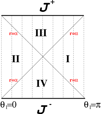
Figure 2: Penrose diagram of de Sitter spacetime. Each point represents a $(n-2)$-sphere except for the two vertical lines at $\theta_{1}=0,\pi$. With respect to the chosen time coordinate we show the static regions I and II and the non-static ones III and IV. Observe that de Sitter spacetime is homogeneous and therefore all its points are equivalent. This would be clearer if we replace each horizontal line by a circle —representing the $S^{n-1}$—in the same manner as in Fig.4. Then the conformal diagram will be given only by the surface of the resulting truncated cylinder. In that case, all points will be equivalent and we can clearly choose the origin of coordinates at any vertical line. With respect to this choice, the coordinates of equation (3) cover any one of the static regions. It is noteworthy to point out the resemblance of the Penrose diagram of each static region with the diagram of Minkowski spacetime. Similarly, the union of any one of the static regions with one of the non-static ones provides the Penrose diagram for the so-called steady state model of the Universe, up to time orientation.

Define the diffeomorphisms $\varphi_{b}:d\mathbb{S}\rightarrow\mathbb{E}$ by $(\bar{t},\bar{\theta_{i}})=(bt,\theta_{i}),\ b>0$. Then

$$\varphi^{*}_{b}\tilde{{\bf g}}=\left(b^{2}-\frac{a^{2}}{\alpha^{2}\cosh^{2}(t/\alpha)}\right)dt\otimes dt+\frac{a^{2}}{\alpha^{2}\cosh^{2}(t/\alpha)}{\bf g}$$

so that by using any of the criteria 1 or 2 one can easily check that $\varphi^{*}_{b}\tilde{{\bf g}}\in{\cal DP}^{+}_{2}(d\mathbb{S})$ if $b^{2}\geq a^{2}/\alpha^{2}$. The corollary 3.1 immediately implies then that $\varphi_{b}$ are causal relations for these values of $b$, so that $d\mathbb{S}\prec\mathbb{E}$. A natural question arises: is $\mathbb{E}\prec d\mathbb{S}$ and thus $d\mathbb{S}\sim\mathbb{E}$? To answer this question one can try to build an explicit causal relation from $\mathbb{E}$ to $d\mathbb{S}$, but one readily realizes that there are no such simple diffeomorphisms. Of course, at this stage one is unsure whether there may be other, yet untried, diffeomorphisms which are the sought causal relations. But the problem is the impossibility to check all the diffeomorphisms explicitly. Nevertheless, we will prove in section 5 that one can find results and criteria allowing to avoid this problem completely, and providing very simple ways to prove, or disprove, the causal relationship between given spacetimes. Thus, we will answer the question of whether or not $d\mathbb{S}\sim\mathbb{E}$ in the Example 6 of section 5.

Example 3

Take again ordinary $n$-dimensional flat spacetime $\mathbb{L}$ but now in spherical coordinates $\{T,R,\theta_{1},\dots,\theta_{n-2}\}$ so that the line element reads

$$(\mathbb{L},{\bf g}):ds^{2}=dT^{2}-dR^{2}-R^{2}d\Omega^{2}_{n-2}$$ (2)

with $-\infty<T<\infty$ and $0<R<\infty$. The second spacetime will be one of the static regions of de Sitter spacetime, denoted here by $\frac{1}{4}d\mathbb{S}$, given by the line element

$$\left(\mbox{$\frac{1}{4}$}d\mathbb{S},\tilde{{\bf g}}\right):d\tilde{s}^{2}=\left(1-\frac{r^{2}}{\alpha^{2}}\right)dt^{2}-\left(1-\frac{r^{2}}{\alpha^{2}}\right)^{-1}dr^{2}-r^{2}d\bar{\Omega}^{2}_{n-2},$$ (3)

where the non-angular coordinate ranges are $-\infty<t<\infty,\ 0<r<\alpha$ (see figure 2). We are going to show that these spacetimes are causally equivalent. To that end, consider the diffeomorphisms $\varphi_{\beta}:\mathbb{L}\rightarrow\frac{1}{4}d\mathbb{S}$ and $\Psi_{f}:\frac{1}{4}d\mathbb{S}\rightarrow\mathbb{L}$ defined by

$$(T,R,\theta_{k})\stackrel{{\scriptstyle\varphi_{\beta}}}{{\longrightarrow}}(T,\frac{\alpha\beta R}{1+\beta R},\theta_{k})$$

$$(t,r,\bar{\theta_{k}})\stackrel{{\scriptstyle\Psi_{f}}}{{\longrightarrow}}(t,f(r),\bar{\theta_{k}})$$

where $\beta$ is a positive constant and $f(r)$ a function to be determined. By writing down $\varphi^{*}_{\beta}\tilde{{\bf g}}$ and $\Psi^{*}_{f}{\bf g}$ in appropriate orthonormal cobases we obtain their eigenvalues with respect to ${\bf g}$ and $\tilde{{\bf g}}$, given respectively by (we shall always write the “timelike” eigenvalue first)

$$\left\{\frac{1+2\beta R}{(1+\beta R)^{2}},\frac{\alpha^{2}\beta^{2}}{(1+\beta R)^{2}(1+2\beta R)},\frac{\alpha^{2}\beta^{2}}{(1+\beta R)^{2}},\dots,\frac{\alpha^{2}\beta^{2}}{(1+\beta R)^{2}}\right\},$$

$$\left\{\left(1-\frac{r^{2}}{\alpha^{2}}\right)^{-1},\left(1-\frac{r^{2}}{\alpha^{2}}\right)f^{\prime 2},\frac{f^{2}}{r^{2}},\dots,\frac{f^{2}}{r^{2}}\right\}.$$

By using now criterion 2 we can write down the conditions for $\varphi^{*}_{\beta}\tilde{{\bf g}}$ and $\Psi^{*}_{f}{\bf g}$ to be in ${\cal DP}^{+}(\mathbb{L})$ and ${\cal DP}^{+}(\frac{1}{4}d\mathbb{S})$ respectively:

$$\varphi^{*}_{\beta}\tilde{{\bf g}}\in{\cal DP}^{+}_{2}(\mathbb{L})\Longleftrightarrow\beta^{2}\leq\frac{1}{\alpha^{2}}$$ (4)

$$\Psi^{*}_{f}{\bf g}\in{\cal DP}^{+}_{2}(\mbox{$\frac{1}{4}$}d\mathbb{S})\Longleftrightarrow\left(1-\frac{r^{2}}{\alpha^{2}}\right)^{-2}\geq f^{\prime 2},\ \left(1-\frac{r^{2}}{\alpha^{2}}\right)^{-1}\geq\frac{f^{2}}{r^{2}}.$$ (5)

Condition (4) is clearly satisfied choosing the values of $\beta$, while condition (5) is easily seen to be fulfilled for suitable choices of $f(r)$. One such choice is, for instance, $f(r)=-br\log\left|1-\frac{r^{2}}{\alpha^{2}}\right|$, for adequate values of the constant $b$. Finally, corollary 3.1 ensures then that $\frac{1}{4}d\mathbb{S}\sim\mathbb{L}$.

This example illustrates how two Lorentzian manifolds with different global and metric properties can be isocausal. Notice that $\frac{1}{4}d\mathbb{S}$ is geodesically incomplete while $\mathbb{L}$ is b-complete (see [1, 18, 38]), and nevertheless they are isocausal. As we see from figures 1 and 2, the Penrose diagrams of both spacetimes have a similar “shape”. We will provide further examples, starting with the next Example 4, showing that this happens in general for causally equivalent spacetimes if their Penrose conformal diagrams are defined. Thereby, the causal equivalence can provide an adequate generalization, for cases in which the Penrose diagrams cannot be drawn, of these very useful drawings/representations of spacetimes. We will present several examples in this paper.

Example 4

Let us consider the $n$-dimensional Robertson-Walker spacetimes $\mathbb{R}\mathbb{W}_{k}$ [18, 38] for the case of flat spatial sections ($k=0$) and such that the equation of state for the cosmological perfect fluid is $p=\gamma\rho$ where $p$ is the isotropic pressure, $\rho$ is the energy density and $\gamma$ is a constant. Solving the Einstein equations under these hypotheses the scale factor takes the form $a(t)=Ct^{\frac{2}{(n-1)(1+\gamma)}}$ where $C$ is a constant and $\gamma\neq-1$, see e.g. [38] for $n=4$. Hence the line-element is given by

$$(\mathbb{R}\mathbb{W}_{0}\{\gamma\},\tilde{{\bf g}}):\ d\tilde{s}^{2}=dt^{2}-C^{2}t^{\frac{4}{(n-1)(1+\gamma)}}(d\chi^{2}+\chi^{2}d\bar{\Omega}^{2}_{n-2}),\,\,0<t,\chi<\infty.$$ (6)

The Penrose diagrams of these spacetimes are shown in figure 3 for every value of $\gamma$.

Figure 3: Penrose diagrams of $\mathbb{R}\mathbb{W}_{0}\{\gamma\}$ spacetimes for $\gamma\in(-\infty,-1)\cup(\frac{3-n}{n-1},\infty)$ (case a), $-1<\gamma<\frac{3-n}{n-1}$ (case b), and $\gamma=\frac{3-n}{n-1}$ (case c). Notice the similar shape of these diagrams with that of Minkowski spacetime (case c) and of the steady state spacetime up to time orientation (cases a and b).

The exceptional case $\gamma=-1$ is in fact the part of de Sitter universe $d\mathbb{S}$ usually called the “steady state” model in General Relativity [18] and shown in figure 2, which we will denote here by $\frac{1}{2}d\mathbb{S}=\mathbb{R}\mathbb{W}_{0}\{-1\}$. Its line-element reads

$$\left(\mbox{$\frac{1}{2}$}d\mathbb{S}_{\pm},{\bf g}\right):\,\,ds^{2}=dT^{2}-e^{\pm 2T/\alpha}(dR^{2}+R^{2}d\Omega^{2}_{n-2}),\hskip 8.53581pt-\infty<T<\infty,\ 0<R<\infty\,$$ (7)

where now the coordinates cover only the regions II and IV (for the minus sign), or II and III (for the plus sign), of the full de Sitter spacetime shown in figure 2.

As conjectured in the previous example, spacetimes with equal-shaped conformal diagrams will be isocausal. Therefore, from figures 2 and 3 we guess that $\mathbb{R}\mathbb{W}_{0}\{\gamma\in(-1,\frac{3-n}{n-1})\}$ will be isocausal to $\frac{1}{2}d\mathbb{S}_{+}$ (with the plus sign), while $\mathbb{R}\mathbb{W}_{0}\{\gamma\notin[-1,\frac{3-n}{n-1}]\}$ will be isocausal to $\frac{1}{2}d\mathbb{S}_{-}$ . The remaining case $\gamma=\frac{3-n}{n-1}$ has a diagram which is in fact similar to that of $\frac{1}{4}d\mathbb{S}$, i.e. the static region II of de Sitter spacetime, see figure 2, which we already know to be isocausal to flat spacetime $\mathbb{L}$. Thus, $\mathbb{R}\mathbb{W}_{0}\{\frac{3-n}{n-1}\}$ will be isocausal to $\mathbb{L}$. We are now going to prove that all these conjectures are actually true.

To that end, and without loss of generality, we put $C=1$ in (6) and $\alpha=1$ in (7). The candidate diffeomorphisms $\varphi_{b,c}:\mathbb{L}\longrightarrow\mathbb{R}\mathbb{W}_{0}\{\gamma\}$, or $\varphi_{b,c}:\frac{1}{2}d\mathbb{S}_{\pm}\longrightarrow\mathbb{R}\mathbb{W}_{0}\{\gamma\}$, will be defined by

$$(T,R,\theta_{i})\stackrel{{\scriptstyle\varphi_{b,c}}}{{\longrightarrow}}(be^{cT},R,\theta_{i})$$

for some constants $b$ and $c>0$. Thus we respectively get

$$\varphi^{*}_{b,c}\tilde{{\bf g}}=\left(b^{2}c^{2}e^{2cT}-K\exp\left(\frac{4Tc}{(n-1)(1+\gamma)}\right)\right)dT\otimes dT+K\exp\left(\frac{4Tc}{(n-1)(1+\gamma)}\right){\bf g}|_{\mathbb{L}}$$

$$\varphi^{*}_{b,c}\tilde{{\bf g}}=\left(b^{2}c^{2}e^{2cT}\!\!\!-K\exp\left(\frac{4cT}{(n-1)(1\!+\!\gamma)}\!\mp\!\!2T\right)\right)dT\otimes dT+K\exp\left(\frac{4cT}{(n-1)(1\!+\!\gamma)}\!\mp\!\!2T\right){\bf g}|_{\frac{1}{2}d\mathbb{S}_{\pm}}$$

where $K=b^{\frac{4}{(n-1)(1+\gamma)}}$. Therefore, using criteria 1 or 2, $\varphi^{*}\tilde{{\bf g}}\in{\cal DP}^{+}_{2}(\mathbb{L})$ in the first case if and only if $b^{2}c^{2}e^{2cT}\geq K\exp\left(\frac{4c}{(n-1)(1+\gamma)}T\right)$ holds for every value of $T$, and this happens only if $\gamma=\frac{3-n}{n-1}$ and $c^{2}\geq 1$. Choosing $c=b=1$ (say), from corollary 3.1 we have $\mathbb{L}\prec_{\varphi_{1,1}}\mathbb{R}\mathbb{W}_{0}\{\frac{3-n}{n-1}\}$. Notice that in this case we have then $\varphi^{*}_{1,1}\tilde{{\bf g}}\propto{\bf g}$, i.e., $\varphi_{1,1}$ is a conformal relation, see the next section. In this case $\varphi^{-1}_{1,1}$ is also a causal relation, as can be easily checked, and therefore $\mathbb{L}\sim\mathbb{R}\mathbb{W}_{0}\{\frac{3-n}{n-1}\}$.

Similarly, $\varphi^{*}_{b,c}\tilde{{\bf g}}\in{\cal DP}^{+}_{2}(\frac{1}{2}d\mathbb{S}_{\pm})$ in the second case if and only if, $\forall T\in(-\infty,\infty)$, $b^{2}c^{2}\geq K\exp\left[\left(\frac{4c}{(n-1)(1+\gamma)}\mp 2-2c\right)T\right]$ which holds for appropriate values of $b$ whenever $c=\mp\frac{(n-1)(1+\gamma)}{n-3+(n-1)\gamma}$. As $c$ must be a positive constant so that the causal orientations are made consistent, we must choose the plus sign for $\gamma\in(-1,\frac{3-n}{n-1})$ and the minus sign for $\gamma\notin[-1,\frac{3-n}{n-1}]$. If we choose $b$ such that $b^{2}c^{2}=K$ then the inverse diffeomorphism is also a causal relation and we have $\frac{1}{2}d\mathbb{S}_{-}\sim\mathbb{R}\mathbb{W}_{0}\{\gamma\notin[-1,\frac{3-n}{n-1}]\}$, and $\frac{1}{2}d\mathbb{S}_{+}\sim\mathbb{R}\mathbb{W}_{0}\{\gamma\in(-1,\frac{3-n}{n-1})\}$.

4 Canonical null directions of causal relations. Conformal relations

As was already pointed out, if $\varphi$ is a causal relation between $V$ and $W$, then the Lorentzian cone of a point in $V$ is mapped by means of $\varphi$ within the Lorentzian cone of the image point of $W$. Nevertheless, as we have seen in the previous example, there are cases in which the causal relations are conformal and then the null cones (that is, the boundaries of the Lorentz cones) are preserved. In general, a part of the initial null cone may or may not remain on the final null cone by the application of $\varphi$, but those parts which do remain can be identified easily by means of the next result.

Proposition 4.1

Let $V\prec_{\varphi}W$ and $\vec{X}\in\Theta^{+}_{x}$. Then $\varphi^{\prime}\vec{X}\in\partial\Theta^{+}_{\varphi(x)}$ if and only if $\vec{X}$ is a null eigenvector of $\varphi^{*}\tilde{{\bf g}}|_{x}$.

Proof :    Let $\vec{X}$ be an element of $\Theta^{+}_{x}$ and suppose $\varphi^{\prime}\vec{X}$ is null at $\varphi(x)$. Then according to proposition 3.2 $\vec{X}$ is also null at $x$. On the other hand we have

$$0=\tilde{{\bf g}}|_{\varphi(x)}(\varphi^{{}^{\prime}}\vec{X},\varphi^{{}^{\prime}}\vec{X})=\varphi^{*}\tilde{{\bf g}}|_{x}(\vec{X},\vec{X})$$

and since $\varphi^{*}\tilde{{\bf g}}|_{x}\in{\cal DP}^{+}_{2}(x)$, lemma 2.2 implies that $\vec{X}$ is a null eigenvector of $\varphi^{*}\tilde{{\bf g}}$ at $x$. The converse is trivial.

The existence of null vectors which remain null under the application of a causal relation motivates the next definition.

Definition 4.1

If the relation $V\prec_{\varphi}W$ holds and $\varphi^{*}\tilde{{\bf g}}$ possesses $m$ independent null eigenvectors $\forall x\in V$, these are called the canonical null directions of $\prec_{\varphi}$.

Remarks

• The importance of proposition 4.1 and definition 4.1 lies on the recently proved fact that the null eigenvectors of any tensor in ${\cal DP}^{+}_{2}$ thoroughly classify it by means of its canonical decomposition found in [2]. The relevant result here is Theorem 4.1 of [2], which can be summarized as

  Theorem 4.1

  Every ${\bf T}\in{\cal DP}^{+}_{2}(V)$ can be written canonically as the sum ${\bf T}=\sum^{n}_{r=1}{\bf S}\{{\bf\Omega}_{[r]}\}$ of rank-2 “super-energy tensors” ${\bf S}\{{\bf\Omega}_{[r]}\}\in{\cal DP}^{+}_{2}(V)$ of simple $r$-forms ${\bf\Omega}_{[r]}$. Furthermore, the decomposition is characterized by the null eigenvectors of ${\bf T}$ as follows: if ${\bf T}$ has $m$ linearly independent null eigenvectors $\vec{k}_{1},\dots,\vec{k}_{m}$ then the sum starts at $r=m$ and ${\bf\Omega}_{[m]}={\bf k}_{1}\wedge\dots\wedge{\bf k}_{m}$; if ${\bf T}$ has no null eigenvector then the sum starts at $r=1$ and $\vec{\Omega}_{[1]}$ is the timelike eigenvector of ${\bf T}$.

  For the sake of completeness, let us recall that the super-energy tensor of an arbitrary $r$-form ${\bf\Lambda}$ is given by the formula [39]:

  $$S_{ab}\{{\bf\Lambda}\}=\frac{(-1)^{r-1}}{(r-1)!}\left[\Lambda_{aa_{2}\dots a_{r}}\Lambda_{b}^{\ a_{2}\dots a_{r}}-\frac{1}{2r}\Lambda_{a_{1}\dots a_{n}}\Lambda^{a_{1}\dots a_{n}}\mbox{g}_{ab}\right]$$ (8)

  and in general they satisfy ${\bf S}\{{\bf\Lambda}\}\in{\cal DP}^{+}_{2}(V)$ and $S_{ab}\{{\bf\Lambda}\}=S_{ba}\{{\bf\Lambda}\}$. If ${\bf\Lambda}$ is a simple $r$-form then ${\bf S}\{{\bf\Lambda}\}$ is proportional to an involutory Lorentz transformation because $S_{ac}S^{c}_{\ b}\propto\mbox{g}_{ab}$. We deduce from this theorem and equation (8) that any tensor of ${\cal DP}^{+}_{2}(V)$ possessing $\it n$ independent null eigenvectors is the metric tensor up to a positive factor. See [2] for further details.

• Therefore, if $V\prec_{\varphi}W$ then $\varphi^{*}\tilde{{\bf g}}$ (which is in ${\cal DP}^{+}_{2}(V)$ by theorem 3.1) admits always a decomposition of the type shown in theorem 4.1, and the number of its canonical null directions, if there are any, is given by the number $r$ where that sum starts.

With the aid of the previous remarks we get an important theorem which characterizes the conformal relations among the set of all causal relations between Lorentzian manifolds.

Theorem 4.2

For a diffeomorphism $\varphi:V\longrightarrow W$ the following properties are equivalent, characterizing the conformal relations:

1. $\varphi$ is a causal (or anticausal) relation with $n$ canonical null directions.

2. $\varphi^{*}\tilde{{\bf g}}=\lambda{\bf g}$, $\lambda>0$.

3. $(\varphi^{-1})^{*}{\bf g}=\mu\tilde{{\bf g}}$, $\mu>0$.

4. $\varphi$ and $\varphi^{-1}$ are both causal (or both anticausal) relations.

Proof :

$(i)\Rightarrow(ii)$ If $\varphi$ is a causal relation with $n$ independent canonical null directions, then $\varphi^{*}\tilde{{\bf g}}\in{\cal DP}^{+}_{2}(V)$ has $n$ independent null eigenvectors which is only possible, according to theorem 4.1 and its remarks, if $\varphi^{*}\tilde{{\bf g}}=\lambda{\bf g}$ for some positive function $\lambda$ defined on $V$.

$(ii)\Leftrightarrow(iii)$ If $\varphi^{*}\tilde{{\bf g}}=\lambda{\bf g}$, then $\tilde{{\bf g}}=(\varphi\circ\varphi^{-1})^{*}\tilde{{\bf g}}=(\varphi^{-1})^{*}\varphi^{*}\tilde{{\bf g}}=(\varphi^{-1})^{*}(\lambda{\bf g})$. The converse is similar.

$(iii)\Rightarrow(iv)$ Theorem 3.1 together with $(ii)$ and $(iii)$ imply $(iv)$ immediately.

$(iv)\Rightarrow(i)$ If $(iv)$ holds, we can establish the following assertion by application of proposition 3.2 to $\varphi^{-1}$

$$(\varphi^{-1})^{{}^{\prime}}\vec{Y}\in\Theta^{+}(V)\ \mbox{is null and $\vec{Y}\in\Theta^{+}(W)$}\Longrightarrow\vec{Y}\ \mbox{is null}.$$

Now, let $\vec{X}\in\Theta^{+}(V)$ be null and consider the unique $\vec{Y}\in T(W)$ such that $\vec{X}=(\varphi^{-1})^{{}^{\prime}}\vec{Y}$. Then $\vec{Y}=\varphi^{{}^{\prime}}\vec{X}$ and $\vec{Y}\in\Theta^{+}(W)$ because $\varphi$ is a causal relation (the anticausal case is similar). According to the assertion above $\vec{Y}$ must then be null and we conclude that every null $\vec{X}\in\Theta^{+}(V)$ is push-forwarded to a null vector of $\Theta^{+}(W)$. Thus, proposition 4.1 implies in fact that all null vectors are eigenvectors of $\varphi^{*}{\bf g}$.

This theorem fully characterizes the (time-preserving) conformal relations as those diffeomorphisms mapping null future-directed vectors onto null future-directed vectors. It is worth remarking here that there are a number of results characterizing conformal relations as the homeomorphisms preserving the null geodesics, see [19], [20].

Observe that theorem 4.2 implies that $V\prec_{\varphi}W$ and $W\prec_{\varphi^{-1}}V$ hold if and only if $\varphi$ is a conformal relation. Thus, as was naturally expected, if $\varphi:V\rightarrow W$ is a conformal relation, then $V\sim W$. However, the converse does not hold in general, and there are isocausal spacetimes which are not conformally related. This happens when $V\prec_{\varphi}W$ and $W\prec_{\psi}V$, but $W\nprec_{\varphi^{-1}}V$. In consequence, the causal equivalence is a generalization of the conformal relation between Lorentzian manifolds.

A door open by theorem 4.2 is the question of whether one can consistently define the concept of “partly conformal” Lorentzian manifolds among those which are isocausal. The idea here is to explore the possibility of having conformally related subspaces without the full manifolds being conformal. This idea can be made precise as follows

Definition 4.2

If $V\sim W$, we shall say that $V$ and $W$ are $\frac{m}{n}$-conformally related if there are causal relations $V\prec_{\varphi}W$ and $W\prec_{\psi}V$ with $m$ corresponding canonical null directions.

Remarks

• By “corresponding” canonical null directions we mean that $m$ null eigenvectors of $\varphi^{*}\tilde{{\bf g}}$ are mapped by $\varphi$ to $m$ null eigenvectors of $\psi^{*}{\bf g}$, and vice versa.

• In general, two isocausal spacetimes are not conformally related at all. However, if they are $\frac{m}{n}$-conformally related, then they are $\frac{s}{n}$-conformally related for all natural numbers $s\leq m$. Thus, the sensible thing to do is to speak about $\frac{m}{n}$-conformal relations only for the maximum value of $m$.

• Obviously, the $\frac{n}{n}$-conformal relation is just the conformal relation. We know that two locally conformal spacetimes are characterized by the preservation of the so-called conformal (Weyl) curvature tensor [18, 7]. The generalization to the case of partial conformal relations is under current investigation [10].

Example 5

Consider the general form of the line-element for the so-called “pp-waves”, see e.g. [22, 21], given in general dimension $n$ by

$$ds^{2}=2dudv-\sum_{k=2}^{n-1}(dx^{k})^{2}+2H_{1}(u,x^{k})du^{2},\ -\infty<u,v,x^{k}<\infty.$$ (9)

The base manifold of these spacetimes is $\mathbb{R}^{n}$ and we will denote them by $pp\mathbb{W}(H_{1})$. Let $pp\mathbb{W}(H_{2})$ be another pp-wave spacetime with a different function $H_{2}$ and coordinates $\{\bar{u},\bar{v},\bar{x}^{k}\}$. To compare them causally, take the diffeomorphisms $\varphi_{f}:(pp\mathbb{W}(H_{1}),{\bf g})\rightarrow(pp\mathbb{W}(H_{2}),\tilde{{\bf g}})$ and $\psi:(pp\mathbb{W}(H_{2}),\tilde{{\bf g}})\rightarrow(pp\mathbb{W}(H_{1}),{\bf g})$ as follows:

$$(u,v,x^{k})\stackrel{{\scriptstyle\varphi_{f}}}{{\longrightarrow}}(u,v+f(u),x^{k}),\hskip 28.45274pt(\bar{u},\bar{v},\bar{x}^{k})\stackrel{{\scriptstyle\psi}}{{\longrightarrow}}(\bar{u},\bar{v},\bar{x}^{k})$$

so that a simple calculation gives

$$\varphi_{f}^{*}\tilde{{\bf g}}={\bf g}+2\left(H_{2}-H_{1}+f^{\prime}(u)\right)\,{\bf k}\otimes{\bf k},\hskip 28.45274pt\psi^{*}{\bf g}=\tilde{{\bf g}}+2(H_{1}-H_{2})\,\bar{{\bf k}}\otimes\bar{{\bf k}}$$

where ${\bf k}=du$ is a future-directed null 1-form in $pp\mathbb{W}(H_{1})$ and the same for ${\bar{\bf k}}=d\bar{u}$. It is then clear, by using criterion 1, that $\varphi_{f}^{*}\tilde{{\bf g}}\in{\cal DP}^{+}(pp\mathbb{W}(H_{1}))$ if and only if $H_{2}-H_{1}+f^{\prime}\geq 0$, and that $\psi^{*}{\bf g}\in{\cal DP}^{+}(pp\mathbb{W}(H_{2}))$ iff $H_{1}-H_{2}\geq 0$. Hence, due to corollary 3.1, the two pp-wave spacetimes will be isocausal if, for instance,

$$0\leq H_{1}-H_{2}\leq f^{\prime}(u).$$

There are many possibilities to comply with such conditions, one simple example is $H_{1}-H_{2}=\sin^{2}F$ and $f(u)=\sinh u$, where $F(u,x^{k})$ is an arbitrary function. In this case, they are in fact $\frac{1}{n}$-conformally related, because the null vectors $\vec{k}$ and $\vec{\bar{k}}$ are corresponding canonical null directions for those diffeomorphisms, as can be easily checked: they are null eigenvectors of $\varphi_{\sinh u}^{*}\tilde{{\bf g}}$ and $\psi^{*}{\bf g}$, respectively.

We may note in passing that this can be used to provide an explicit example of a pair of isocausal spacetimes not conformally related (not even locally). For if we take $H_{2}=0$ so that $pp\mathbb{W}(0)=\mathbb{L}$ is Minkowski spacetime, the condition for isocausality becomes $0\leq H_{1}\leq f^{{}^{\prime}}(u)$ and it is very easy to choose $H_{1}$ in such a way that $pp\mathbb{W}(H_{1})$ is not locally conformally flat.

5 Applications to causality theory

In this section we study how the causal properties of two Lorentzian manifolds $V$ and $W$ are related when $V\prec W$. For that purpose, let us recall the basic sets used in causality theory [1, 18, 38, 44]. If $p,q\in V$, $p<q$ means that there exists a continuous future-directed causal curve from $p$ to $q$, and similarly for $p<\!\!<q$ if the curve can be timelike. Then the chronological and causal futures of any point $p$ are defined respectively by [18]

$$I^{+}(p)=\{x\in V:p<\!\!<x\},\ \ J^{+}(p)=\{x\in V:p<x\}$$

and dually for the past. These definitions are translated in an obvious way to arbitrary sets $\zeta\subset V$ and so we write $I^{\pm}(\zeta)$ and $J^{\pm}(\zeta)$. A set $\zeta$ is called a future set if $I^{+}(\zeta)\subseteq\zeta$. For example $I^{+}(\zeta)$ is a future set for any $\zeta$. A set $\zeta$ is achronal if $\zeta\cap I^{+}(\zeta)=\emptyset$, and acausal if there are no points $p,q\in\zeta$ such that $p<q$ (this implies that $\zeta\cap J^{+}(\zeta)=\zeta$, but is not equivalent to that in general.) The boundary of a future set is always achronal and is called an achronal boundary. Due to the connectedness of the manifold, $V$ can be disjointly decomposed as $V={\cal B}^{+}\cup{\cal B}\cup{\cal B}^{-}$ where ${\cal B}^{+}$ is any open future set, ${\cal B}$ its achronal boundary, and ${\cal B}^{-}=\mbox{ext}{\cal B}^{+}$ is a past set. Of course ${\cal B}$ is also the achronal boundary for ${\cal B}^{-}$. Finally we must also recall the definitions of the future and past Cauchy developments. Let $\gamma^{\pm}_{p}$ be a future (past) causal curve passing through $p$ and denote by $\Gamma^{\pm}_{p}$ the set of all such endless curves. The future Cauchy development of $\zeta$ is defined as follows

$$D^{+}(\zeta)=\{x\in V:\,\gamma^{-}_{x}\cap\zeta\neq\emptyset\ \forall\gamma^{-}_{x}\in\Gamma^{-}_{x}\}$$

and similarly for $D^{-}(\zeta)$. The Cauchy development of $\zeta$ is then $D(\zeta)=D^{+}(\zeta)\cup D^{-}(\zeta)$. All the above concepts are standard, well studied and defined in many references, see for instance [1, 18, 44, 38].

5.1 Causality sets and causal relations

With all the nomenclature now at hand, we can prove several results giving the behaviour of the causality sets under the application of a causal relation between Lorentzian manifolds.

Proposition 5.1

$V\prec_{\varphi}W$ if and only if every continuous future-directed timelike (causal) curve in $V$ is mapped by $\varphi$ to a continuous future-directed timelike (causal) curve in $W$.

Proof :    If every future-directed timelike curve $\gamma\subset V$ is mapped by $\varphi$ to a future-directed timelike curve $\varphi(\gamma)\subset W$, then by choosing the $\gamma$’s to be $C^{1}$ every future-directed timelike tangent vector is mapped to a future-directed timelike vector. As a consequence if $\vec{k}\in T(V)$ is null and future-directed then $\varphi^{\prime}\vec{k}$ must be causal and future-directed (to see this just construct a sequence of future-directed timelike vectors converging to $\vec{k}$.) Conversely, take any continuous future-directed $\gamma\subset V$. It is known that $\gamma$ must be differentiable almost everywhere [31] so that from proposition 3.2 $\varphi(\gamma)$ is continuous and future-directed almost everywhere. Finally, if $\gamma$ is not differentiable at $p\in\gamma$, then there is a normal neighbourhood ${\cal U}_{p}$ of $p$ such that, for every $q,r\in\gamma\cap{\cal U}_{p}$ there is a future-directed differentiable arc from $q$ to $r$. As $V\prec_{\varphi}W$ this arc is mapped to another differentiable arc which is future-directed, so that $\varphi({\cal U}_{p})$ is a normal neighbourhood of $\varphi(p)$ with the required property such that $\varphi(\gamma)$ is also continuous and future-directed at $\varphi(p)$.

Proposition 5.2

If $V\prec_{\varphi}W$ then $\varphi(I^{\pm}(\zeta))\subseteq I^{\pm}(\varphi(\zeta))$ and $\varphi(J^{\pm}(\zeta))\subseteq J^{\pm}(\varphi(\zeta))$ for every set $\zeta\subset V$.

Proof :    It is enough to prove it for a single point $p\in V$ and then getting the result for every $\zeta$ by considering it as the union of its points. For the first relation, let $y$ be in $\varphi(I^{+}(p))$ arbitrary and take $x\in I^{+}(p)$ such that $\varphi(x)=y$. Since $p<\!\!<x$ we can choose a future-directed timelike curve $\gamma$ from $p$ to $x$. From proposition 5.1, $\varphi(\gamma)$ is then a future-directed timelike curve joining $\varphi(p)$ and $y$, so that $y\in I^{+}(\varphi(p))$. The second assertion is proved in a similar way using again proposition 5.1. The proof for the past sets is analogous.

This implies that causal relations are “chronological maps” in the sense of [15].

Proposition 5.3

If $V\prec_{\varphi}W$ and $\zeta\subset W$ is acausal (achronal) then $\varphi^{-1}(\zeta)$ is acausal (achronal).

Proof :    If there were $p,q\in\varphi^{-1}(\zeta)$ such that $p<q$ ($p\neq q$) then proposition 5.2 would imply $\varphi(p)<\varphi(q)$, ($\varphi(p)\neq\varphi(q)$) with $\varphi(p),\varphi(q)\in\zeta$, against the assumption. And similarly for the achronal case.

The impossibility of the existence of causal relations between given Lorentzian manifolds can be proven sometimes by using results relating causality sets or causal curves. The following proposition is an example. Let us recall that, for any inextendible causal curve $\gamma$, the boundaries $\partial I^{\pm}(\gamma)$ of its chronological future and past are usually called its future and past event horizons, sometimes also called creation and particle horizons, respectively [18, 30, 44, 38]. Of course these sets can be empty (then $\gamma$ has no horizon).

Proposition 5.4

Suppose that every inextendible future-directed causal curve in $W$ has a non-empty $\partial I^{-}(\gamma)$ ($\partial I^{+}(\gamma)$). Then any $V$ such that $V\prec W$ cannot have inextendible causal curves without past (future) event horizons.

Proof :    If there were a future-directed curve $\gamma$ in $V$ with $\partial I^{-}(\gamma)=\emptyset$, $I^{-}(\gamma)$ would be the whole of $V$. But according to proposition 5.2 $\varphi(I^{-}(\gamma))\subseteq I^{-}(\varphi(\gamma))$ from what we would conclude that $I^{-}(\varphi(\gamma))=W$ in contradiction.

Example 6

Let us recall Example 2 in section 3, where we proved that $d\mathbb{S}\prec\mathbb{E}$, but we did not know if $\mathbb{E}\prec d\mathbb{S}$. Now, by using proposition 5.4 we have that $\mathbb{E}\not\prec d\mathbb{S}$ because every causal curve in the de Sitter spacetime possesses a non-empty event horizon, see e.g [18], but none of them has one in the Einstein universe. Thus, $\mathbb{E}\not\sim d\mathbb{S}$. This is again clear by taking a look at the corresponding conformal diagrams, shown in Figures 2 and 4. Notice that both $d\mathbb{S}$ and $\mathbb{E}$ are locally conformally flat, and therefore they are metrically conformally related to each other. However, this conformal property is not given by a global diffeomorphism.

Figure 4: Conformal diagram of Einstein spacetime. In this picture the spacetime is represented by the surface of the figure and each horizontal circle corresponds to an $(n-1)$-sphere in the Einstein spacetime. Compare with [43].

Other impossibilities for causal relations arise from the results for Cauchy developments.

Proposition 5.5

If $V\prec_{\varphi}W$ then $D^{\pm}(\varphi(\zeta))\subseteq\varphi(D^{\pm}(\zeta))\,\,\forall\zeta\subseteq V$.

Proof :    It is enough to prove the future case. Let $y\in D^{+}(\varphi(\zeta))$ arbitrary and consider any causal past directed curve $\gamma^{-}_{\varphi^{-1}(y)}\subset V$ containing $\varphi^{-1}(y)$. Since $\gamma^{-}_{\varphi^{-1}(y)}$ is mapped by $\varphi$ to a causal curve passing through $y$, ergo meeting $\varphi(\zeta)$, we have that $\gamma^{-}_{\varphi^{-1}(y)}$ must meet $\zeta$. As $\gamma^{-}_{\varphi^{-1}(y)}$ is arbitrary we conclude that $y\in\varphi(D^{+}(\zeta))$.

Corollary 5.1

If $V\prec_{\varphi}W$ and $\Sigma\subset W$ is a Cauchy hypersurface then $\varphi^{-1}(\Sigma)\subset V$ is a Cauchy hypersurface too.

Proof :    Recall that a Cauchy hypersurface $\Sigma\subset W$ is a closed acausal set without edge such that $D(\Sigma)=W$ [1, 18, 44, 38]. Proposition 5.5 implies then $W=D(\Sigma)\subseteq\varphi(D(\varphi^{-1}(\Sigma)))$. Since $\varphi$ is a diffeomorphism we get that $D(\varphi^{-1}(\Sigma))=V$ and that $\varphi^{-1}(\Sigma)$ has no edge, so that it only remains to prove its acausality. But this is a consequence of proposition 5.3.

Let us also recall that a spacetime is globally hyperbolic if and only if it contains a Cauchy hypersurface [1, 18, 44, 38], see also definition 5.1 below. Thus we also have

Corollary 5.2

If $W$ is globally hyperbolic and $V\prec W$, then $V$ must be globally hyperbolic. Thus, if $W$ is globally hyperbolic but $V$ is not, then $V\nprec W$.

Let us remark that not all diffeomorphic globally hyperbolic spacetimes are isocausal, as seen for instance in Example 6: $\mathbb{E}\not\sim d\mathbb{S}$. The last corollaries are very powerful to discard the causal relationship between many Lorentzian manifolds. Some outstanding cases are presented in the following examples.

Example 7

Let us consider anti-de Sitter spacetime $\mathbb{A}d\mathbb{S}$: $\mathbb{R}^{n}$ with a line-element (in spherical coordinates $\{t,r,\bar{\theta}_{k}\}$) that takes the form

$$(\mathbb{A}d\mathbb{S},\tilde{{\bf g}})\,:\,d\tilde{s}^{2}=\cosh^{2}rdt^{2}-dr^{2}-\sinh^{2}r\,d\bar{\Omega}^{2}_{n-2},\ -\infty<t<\infty,\ 0<r<\infty.$$ (10)

We compare $\mathbb{A}d\mathbb{S}$ with flat spacetime $\mathbb{L}$. By using the standard spherical coordinates of (2) for $\mathbb{L}$ it is very easy to prove that the diffeomorphism $\varphi:\mathbb{L}\rightarrow\mathbb{A}d\mathbb{S}$ which identifies coordinates in a natural way satisfies $\varphi^{*}\tilde{{\bf g}}\in{\cal DP}^{+}_{2}(\mathbb{L})$, so that corollary 3.1 implies that $\varphi$ is a causal relation. Nevertheless, according to corollary 5.2, and since $\mathbb{L}$ is globally hyperbolic but $\mathbb{A}d\mathbb{S}$ is not (see e.g. [18] and figure 5, where the Penrose diagram of $\mathbb{A}d\mathbb{S}$ is shown), we also have that $\mathbb{A}d\mathbb{S}\nprec\mathbb{L}$. Hence, $\mathbb{A}d\mathbb{S}\not\sim\mathbb{L}$. Observe that $\mathbb{A}d\mathbb{S}$ is locally conformally flat with the usual definition, and therefore locally conformally related to $\mathbb{L}$ everywhere. However, this conformal relation cannot be global, as we have just proved in a simple way. Therefore, locally conformally flat spacetimes can have very different causal properties from flat spacetime, and this can be made precise using the concept of causal relationship.

Figure 5: Penrose-like diagram for anti-de Sitter spacetime. In this case we have preferred to draw a 3-dimensional diagram to get a clearer picture of the causal infinity. Every $t=$const. slice has been reduced to an open horizontal disk, so that every point in the diagram represents a $(n-3)$-sphere except for the middle line which is the origin of coordinates. Compare this diagram with that in [18], see also [43]. The boundary of the picture represents the conformal infinity $\cal{J}$ of $\mathbb{A}d\mathbb{S}$. It is remarkable that this boundary has precisely the shape of the Einstein universe, see figure 4. Thus, one is tempted to say that the causal boundary of $n$-dimensional anti-de Sitter spacetime is the $(n-1)$-dimensional Einstein universe. We will try to make the concept of causal boundary precise in section 6. In any case, notice the timelike character of $\cal{J}$ and the non-global hyperbolicity of the $\mathbb{A}d\mathbb{S}$ spacetime.

Example 8

Let us take the particular case of the pp-waves (9) which are pure electromagnetic plane waves: they are locally conformally flat solutions of the Einstein-Maxwell equations; for simplicity we take here $n=4$ [22]. These special plane waves are given by $pp\mathbb{W}(H)$ with $H=\Phi^{2}(u)(x^{2}+y^{2})$, that is

$$\mathbb{P}\mathbb{W}(\Phi):d\bar{s}^{2}=2d\bar{u}d\bar{v}-d\bar{x}^{2}-d\bar{y}^{2}+\Phi^{2}(\bar{u})(\bar{x}^{2}+\bar{y}^{2})d\bar{u}^{2},\ -\infty<\bar{u},\bar{v},\bar{x},\bar{y}<\infty\,.$$

As the manifold is $\mathbb{R}^{4}$ we can try to causally compare these plane waves with flat 4-dimensional spacetime $\mathbb{L}$. Defining the usual advanced and retarded null coordinates the line-element for $\mathbb{L}$ can be written as

$$\mathbb{L}:ds^{2}=2dudv-dx^{2}-dy^{2}\,.$$

Using the diffeomorphism given by $\bar{u}=u,\ \bar{v}=v,\ \bar{x}=x,\ \bar{y}=y$, a calculation analogous to that of the Example 5 proves that $\varphi$ is a causal relation with $\vec{k}$ as canonical null direction. Nevertheless, for all $\Phi\neq 0$ the plane waves $\mathbb{P}\mathbb{W}(\Phi)$ are known to be non-globally hyperbolic [29] and hence the causal relation in the opposite way is not possible. Thus, for all $\Phi\neq 0$, $\mathbb{L}\not\sim\mathbb{P}\mathbb{W}(\Phi)$. Observe that again all the $\mathbb{P}\mathbb{W}(\Phi)$ spacetimes are locally conformally flat, but this does not mean that they are isocausal to $\mathbb{L}$, which is a global property.

5.2 Causally ordered sequences of Lorentzian manifolds. Causal structures

Globally hyperbolic spacetimes are the best-behaved Lorentzian manifolds from the causal point of view and, as we have seen in corollary 5.2, if $W$ has this property and is causally related to $V$, then $V$ must also have it. We can then ask ourselves whether other milder causality conditions behave in a similar way under causal relations. To that end, let us briefly recall here the standard hierarchy of causality conditions [38, 18].

Definition 5.1

A Lorentzian manifold $V$ is said to be:

• not totally vicious if $I^{+}(p)\cap I^{-}(p)\neq V\ \forall p\in V$.

• chronological if $p\not\in I^{+}(p)\ \forall p\in V$.

• causal if $J^{+}(p)\cap J^{-}(p)=\{p\}\ \forall p\in V$.

• future distinguishing if $I^{+}(p)\neq I^{+}(q)$ $\forall p\neq q$, and analogously for the past. This is equivalent to demanding that every neighbourhood of $p$ contains another neighbourhood ${\cal U}_{p}$ of $p$ such that every causal future directed curve starting at $p$ intersects ${\cal U}_{p}$ in a connected set.

• strongly causal if $\forall p\in V$ and for every neighbourhood ${\cal W}_{p}$ of $p$ there exists another neighbourhood ${\cal U}_{p}\subset{\cal W}_{p}$ containing $p$ such that for every causal curve $\gamma$ the intersection $\gamma\cap{\cal U}_{p}$ is either empty or a connected set.

• causally stable if there exists a function whose gradient is timelike everywhere (called a time function).

• globally hyperbolic if it is strongly causal and $J^{+}(p)\cap J^{-}(q)$ is compact for all $p,q\in V$.

These conditions are given with increasing degree of restriction so that any of them implies all the previous. The next result proves that these constraints are kept by causal relations.

Theorem 5.1

Let $V\prec W$. Then, if $W$ satisfies any of the causality conditions of definition 5.1, so does $V$.

Proof :    Let $V\prec_{\varphi}W$. We prove each case separately. If $V$ were totally vicious there would be a $p\in V$ such that $I^{+}(p)=I^{-}(p)=V$, so that from proposition 5.2 $W=\varphi(I^{\pm}(p))\subseteq I^{\pm}(\varphi(p))$ and thus $I^{+}(\varphi(p))\cap I^{-}(\varphi(p))=W$ proving that $W$ would be totally vicious, against the hypothesis.

Suppose $V$ were not a chronological spacetime. Then, from proposition 5.1 $\varphi$ would map every closed timelike curve of $V$ onto a closed timelike curve of $W$, so that $W$ could not be chronological. The proof for a causal spacetime $W$ is similar.

Suppose now that $V$ were not future distinguishing. Then, there would be a point $p\in V$ and a neighbourhood $U_{p}$ of $p$ such that every open set ${\cal U}_{p}$ with $p\in{\cal U}_{p}\subset U_{p}$ would cut at least a causal curve $\gamma$ starting at $p$ in a disconnected set $\gamma\cap{\cal U}_{p}$. But then, using proposition 5.1 again, every open subset of $\varphi(U_{p})$ would also cut the causal curve $\varphi(\gamma)$, which starts at $\varphi(p)$, in a disconnected set, hence $W$ would not be future distinguishing. The past case is identical. The proof for the strongly causal spacetimes is also similar.

Now, let $W$ be causally stable, and let $\tau$ be the function such that $d\tau$ is an everywhere timelike and future directed 1-form. By proposition 3.2 point $(iii)$, $\varphi^{*}(d\tau)=d(\varphi^{*}\tau)$ is also a future-directed timelike 1-form in $V$, and hence $\varphi^{*}\tau$ is the required time function for $V$. Finally, the globally hyperbolic case is corollary 5.2.

We proved in section 3 that the relation $\prec$ is a preorder, hence $(\cal{L},\prec)$, where $\cal{L}$ denotes the class of all Lorentzian manifolds, is a preordered set. Of course, $\prec$ only pre-orders the Lorentzian manifolds which are pairwise diffeomorphic, so that in fact each of the subsets $\mbox{Lor}(M)$ are in fact separately preordered by $\prec$, where $\mbox{Lor}(M)$ denotes the set of Lorentzian manifolds with base manifold $M$. As usual, the equivalence relation constructed from $\prec$, which is the “$\sim$” providing the definition 3.2 of isocausal spacetimes, gives rise to a partial order in the quotient sets $\mbox{Lor}(M)/\!\!\sim$ by means of the new binary relation $\mbox{coset}(V)\preceq\mbox{coset}(W)\Leftrightarrow V\prec W$. Here coset$(V)=\{U\ :\,V\sim U\}$ denotes the equivalence class of spacetimes isocausal to $V$.

All this means that $\cal{L}$, and in fact each of the $\mbox{Lor}(M)$, can be decomposed in disjoint and partially ordered classes of isocausal Lorentzian manifolds. Of course, still we may find classes coset$(V_{1})$ and coset$(V_{2})$ belonging to $\mbox{Lor}(M)/\!\!\sim$ which are not related by $\preceq$ at all. Nevertheless, it is in principle possible to construct causally ordered sequences of spacetimes in which every pair of elements of the sequence are comparable with respect to the binary relation $\preceq$. These sequences look like

$$\mbox{coset}(V)\preceq\dots\preceq\mbox{coset}(W)\preceq\dots\preceq\mbox{coset}(U)\preceq\dots\preceq\mbox{coset}(Z)$$ (11)

where, from theorem 5.1, if a member of the sequence satisfies one of the causality conditions of definition 5.1, then all the previous members (those to the left) comply also with the same condition; and reciprocally, if one of them violates one of those conditions, then all the members to the right violate it too. Since the causality conditions of definition 5.1 are given with increasing order of restriction, we deduce that spacetimes which have stronger causality properties appear towards the left of the sequence, whereas spacetimes with weaker causality conditions appear towards the right of (11). All this is quite natural because the Lorentzian cones open up under a causal relation. It also provides an abstract measure of “increasing causality”: the “smaller” the spacetime in a sequence, the better causal behaviour it has.

The longest sequences of type (11) are those starting with a simple globally hyperbolic spacetime (say a flat space such as $\mathbb{L}$, or equivalently any of the members in coset$(\mathbb{L})$, such as $\frac{1}{4}d\mathbb{S}$ or $\mathbb{R}\mathbb{W}_{0}\{\frac{3-n}{n-1}\}$), passing through a $W$ which is causally stable (say anti de Sitter $\mathbb{A}d\mathbb{S}$, as $\mathbb{L}\prec\mathbb{A}d\mathbb{S}$), and so on until they end with a causally rather badly behaved Lorentzian manifold. Of course, there can be various steps in a sequence with a given property of definition 5.1 (for instance, not all diffeomorphic globally hyperbolic spacetimes are isocausal, e.g., $\mathbb{E}\not\prec d\mathbb{S}$): thus the binary relation $\preceq$ is finer than the classification of definition 5.1. Whether or not the last step in these longest sequences is always a totally vicious spacetime, which would provide a maximal element to the partial order $\preceq$, is an interesting open question. Another question is if there is a minimal element for each sequence, providing the “best” causally behaved spacetime for a given manifold.

All the Lorentzian manifolds involved in a given sequence of type (11) are diffeomorphic to each other, as they belong to $\mbox{Lor}(M)$ and therefore all of them are diffeomorphic to $M$. Consequently, perhaps a more interesting way to look at the previous results is to consider all the classes of equivalence of spacetimes in a sequence as different causal structures on the same manifold $M$. More precisely

Definition 5.2

Let $M$ be a differentiable manifold. A causal structure on $M$ is an equivalence class with respect to $\sim$ of Lorentzian manifolds based at $M$.

Of course, not all manifolds possess a causal structure, for as is well-known not every differentiable manifold possesses a global Lorentzian metric (take for instance $S^{n}$). On the other hand, there are manifolds with many inequivalent causal structures such as for example $\mathbb{R}^{n}$: just consider coset$(\mathbb{L})$, or coset$(\mathbb{A}d\mathbb{S})$, or the equivalence class of Gödel spacetime. Therefore, for any given differentiable manifold admitting causal structures, these can be partially ordered according to $\preceq$ and we can construct sequences of type (11). Interesting open questions are the cardinality of the possible inequivalent causal structures admitted by a given manifold, and the possible existence of minimal and maximal elements.

According to the definition 5.2, two Lorentzian metrics ${\bf g}_{1}$ and ${\bf g}_{2}$ on $M$ are said to be equivalent from the causal point of view if the Lorentzian manifolds $(M,{\bf g}_{1})$ and $(M,{\bf g}_{2})$ are isocausal. In other words, effectively a causal structure on $M$ is simply coset$(V)\subset\mbox{Lor}(M)$ with any of its Lorentzian metrics. Note that specific metric properties (distances, proper times, volumes, etcetera) are completely irrelevant here. An important remark is that our definition of causal structure is more general than the traditional “conformal” one. If one adopts definition 5.2, then the global causal structure of a given Lorentzian manifold is not given up to a conformal factor of the metric. Rather, it only determines coset$(V)$, i.e., the metric up to causal mappings. Whether or not this generalization is adequate depends on the type of properties one wishes to keep. For instance, it is intuitively clear that the causal structure of a weak static gravitational field far from the sources should be similar to that of flat spacetime $\mathbb{L}$. However, no realistic gravitational field will be conformal to $\mathbb{L}$, not even far from the sources. Thus, the conformal structure does not capture the intuitive concept that these two situations share somehow the same causality properties. As we are going to prove in the next examples, the generalization given by definition 5.2 provides a rigorous framework, and a justification, for that intuitive claim.

Example 9

Consider the outer region of $n$-dimensional Schwarzschild spacetime $\mathbb{S}$ in typical spherical coordinates, whose line-element for positive mass $M$ reads

$$d\tilde{s}^{2}=\left(1-\frac{2M}{r^{n-3}}\right)dt^{2}-\left(1-\frac{2M}{r^{n-3}}\right)^{-1}dr^{2}-r^{2}d\bar{\Omega}^{2}_{n-2}$$ (12)

and take the Lorentzian manifolds $\mathbb{S}_{c}$ defined by $-\infty<t<\infty$ and the condition $r>c\geq(2M)^{\frac{1}{n-3}}\equiv c_{M}$. The second spacetime is $\mathbb{L}$ in spherical coordinates as in (2) of Example 3, but in order to make it diffeomorphic with $\mathbb{S}_{c}$ we need to take only a subregion $\mathbb{L}_{a}$ defined by the condition $R>a$ for a fixed non-negative constant $a$.

We want to study the causal relationship between $(\mathbb{S}_{c},\tilde{{\bf g}})$ and $(\mathbb{L}_{a},{\bf g})$. To than end, and to avoid unnecessary writing, we will omit the angular coordinates in what follows, as they are simply identified for all diffeomorphisms under consideration. Define first $\varphi_{b}:\mathbb{L}_{a}\rightarrow\mathbb{S}_{c}$ by $t=bT,\ r=R-a+c$ where $b$ is a positive constant. A simple computation provides the eigenvalues of $\varphi_{b}^{*}\tilde{{\bf g}}$ with respect to ${\bf g}$, given by

$$b^{2}\left(1-\frac{2M}{(R-a+c)^{n-3}}\right),\,\left(1-\frac{2M}{(R-a+c)^{n-3}}\right)^{-1},\,\mbox{and}\,\,\left(\frac{R-a+c}{R}\right)^{2}.$$

Thus if $\varphi_{b}^{*}\tilde{{\bf g}}$ is to be in ${\cal DP}^{+}_{2}(\mathbb{L}_{a})$, according to criterion 2 the following inequalities must hold:

$$b^{2}\left(1-\frac{2M}{(R-a+c)^{n-3}}\right)\geq\left\{\left(1-\frac{2M}{(R-a+c)^{n-3}}\right)^{-1},\ \left(\frac{R-a+c}{R}\right)^{2}\right\}.$$

These can be satisfied for every $c>c_{M}$ by arranging $b$ appropriately. Hence, according to corollary 3.1 we deduce $\mathbb{L}_{a}\prec\mathbb{S}_{c}$ for all $c>c_{M}$.

Reciprocally, let $\psi:\mathbb{S}_{c}\rightarrow\mathbb{L}_{a}$ be defined simply by means of $T=t,R=r$. Then the eigenvalues of $\psi^{*}{\bf g}$ with respect to $\tilde{{\bf g}}$ are given by $\left(1-\frac{2M}{r^{n-3}}\right)^{-1}$, $1-\frac{2M}{r^{n-3}}$ and $1$. Criterion 2 implies that $\psi^{*}{\bf g}\in{\cal DP}^{+}_{2}(\mathbb{S}_{c})$ for every $c\geq c_{M}$ as long as $a\geq c_{M}$, and corollary 3.1 leads to $\mathbb{S}_{c}\prec\mathbb{L}_{c}$ for all $c\geq c_{M}$. The conclusion is that $\mathbb{S}_{c}\sim\mathbb{L}_{c}$ if $c>c_{M}$, as was to be expected. This example can be repeated for a global spacetime $\hat{\mathbb{S}}_{c}$ —formed by Schwarzschild exterior matched to some adequate interior at $c>c_{M}$— and the whole of Minkowski spacetime $\mathbb{L}$. The two manifolds are then diffeomorphic. The conclusion again is that $\hat{\mathbb{S}}_{c}\sim\mathbb{L}$ if $c>c_{M}$.

Notice that $\mathbb{S}_{c}$ is not locally conformally flat, and therefore is not conformal to $\mathbb{L}_{c}$. This means that the conformal structure does not allow to say that $\mathbb{S}_{c}$ and $\mathbb{L}_{c}$ have a similar causality, while the concept of isocausality certainly does, at least up to a point, because $\mathbb{S}_{c}\in$ coset$(\mathbb{L}_{c})$. Since $\mathbb{S}_{c}\sim\mathbb{L}_{c}$, some causal features are shared by these two spacetimes, but of course not all thinkable causal properties. For instance, in $\mathbb{S}$ there are circular null geodesics at $r=[(n-1)/2]^{\frac{1}{n-3}}c_{M}$, but there are clearly none in $\mathbb{L}$. A more drastic example is given by the following property [32]: for all endless causal curves $\gamma_{1}$ and $\gamma_{2}$ in $\mathbb{S}$, $I^{+}(\gamma_{1})\cap\gamma_{2}\neq\emptyset$, and similarly for the past. This could be termed as a causal property, but it is not shared by $\mathbb{L}$, as there are some simple examples in Minkowski spacetime of endless timelike curves which are completely causally disconnected, see [32]. In a way, this is a consequence of the existence of a gravitational field in $\mathbb{S}$, maybe weak, but non-vanishing nonetheless. Such kind of properties could only be kept by the fully faithful conformal structure, but then one would lose the possibility of giving a meaning to the intuitive concept of having close-to-Minkowskian causality in weak fields far from the sources.

With isocausality we have kept, for instance, the causal stability of both $\mathbb{S}_{c}$ and $\mathbb{L}_{c}$, or the global hyperbolicity of $\hat{\mathbb{S}}_{c}$ and $\mathbb{L}$, in a precise mutual way. This can be highlighted by noting the following remark, which also has physical implications: we have not proved $\mathbb{S}_{c}\sim\mathbb{L}_{c}$ for the extreme value $c=c_{M}$, since $\varphi_{b}$ failed to be causal relations in that case. In fact, we can disprove $\mathbb{L}_{a}\prec\mathbb{S}_{c_{M}}$ $\forall a\geq 0$ by making use of corollary 5.2, because $\mathbb{S}_{c_{M}}$ is globally hyperbolic but $\mathbb{L}_{a\geq 0}$ is not (recall also that the manifolds $\mathbb{S}_{c}$ and $\mathbb{L}$ are not diffeomorphic). We conclude then that $\mathbb{L}_{a}\not\prec\mathbb{S}_{c_{M}}$. This is a very interesting result, being a clear manifestation of the null character of the event horizon $r=c_{M}$ in the extensions through it of Schwarzschild’s spacetime. It is remarkable that we have not made direct use of any extension or extendibility of $\mathbb{S}_{c_{M}}$ to achieve this result (although we have clearly used its global hyperbolicity). Once again, a clear picture of what is happening can be obtained by taking a look at the Penrose diagrams, corresponding to the part to the right of $r=a$ in figure 1 for $\mathbb{L}_{a}$ and to the one presented in figure 6. Another example of this type is provided next.

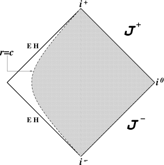
Figure 6: Penrose diagram of the exterior region of Schwarzschild spacetime. Only the part to the right of $r=c$ (shaded zone) is the spacetime $\mathbb{S}_{c}$ which is isocausal to $\mathbb{L}_{c}$. In this case, as is clear from the figure, $\mathbb{S}_{c}$ is not globally hyperbolic. On the other hand, the limit case with $c=c_{M}$, in which the boundary of the spacetime is the event horizon EH, is globally hyperbolic. This spacetime is not isocausal to any part $\mathbb{L}_{a}$ of flat spacetime.

Example 10

In this example we will prove that the outer regions of Schwarzschild ($\mathbb{S}$) and Reissner-Nordström ($\mathbb{R}\mathbb{N}$) black holes in $n$ dimensions are isocausal. In order to avoid complications arising from the parameters which appear in the line element of these spacetimes, we will use spherical dimensionless coordinates in which the line elements take the form:

$$(\mathbb{S},{\bf g}):ds^{2}=\bar{\alpha}^{2}\left[\left(1-\frac{1}{r^{n-3}}\right)dt^{2}-\left(1-\frac{1}{r^{n-3}}\right)^{-1}dr^{2}-r^{2}d\Omega^{2}_{n-2}\right],$$

$$(\mathbb{R}\mathbb{N},\tilde{{\bf g}}):d\tilde{s}^{2}=\alpha^{2}\left[\left(\frac{1}{r_{0}^{n-3}}-\frac{1}{R^{n-3}}\right)\left(\frac{1}{r_{1}^{n-3}}-\frac{1}{R^{n-3}}\right)dT^{2}-\right.$$

$$-\left.\left(\frac{1}{r_{0}^{n-3}}-\frac{1}{R^{n-3}}\right)^{-1}\left(\frac{1}{r_{1}^{n-3}}-\frac{1}{R^{n-3}}\right)^{-1}dR^{2}-R^{2}d\bar{\Omega}^{2}_{n-2}\right],$$

where $\alpha=Q$ is the charge of $\mathbb{R}\mathbb{N}$ and $\bar{\alpha}=2M$ is the mass of $\mathbb{S}$ (we have arranged the original metrics of both black holes in such a way that $M$ and $Q$ have dimensions of length). The parameters $r_{0}$ and $r_{1}$ correspond respectively to the usual Cauchy and event horizons $r_{-}$ and $r_{+}$ of the $\mathbb{R}\mathbb{N}$ black hole by means of the relations $r_{-}=Qr_{0}$ and $r_{+}=Qr_{1}$. We are only interested here in the outer regions of both spacetimes, that is to say, $r>1$ for $\mathbb{S}$ and $R>r_{1}$ for $\mathbb{R}\mathbb{N}$, which are globally hyperbolic. These regions are covered by the previous coordinate systems with the time coordinates $t$ and $T$ running over the whole real line. It is then very easy to write down diffeomorphisms which set up the mutual causal relation. Omitting the angular variables as before, we can choose $\varphi_{b}:\mathbb{S}\rightarrow\mathbb{R}\mathbb{N}$ defined by $T=bt,\ R=r_{1}r$ and $\psi_{a}:\mathbb{R}\mathbb{N}\rightarrow\mathbb{S}$ by $t=aT,\ r=R-r_{1}+1$. A calculation similar to those performed in previous examples, and use of either of the criteria 1 or 2, allows us to find the conditions for the tensors $\varphi^{*}_{b}\tilde{{\bf g}}$ and $\psi^{*}_{a}{\bf g}$ to be causal:

$$\left(\frac{1}{r_{0}^{n-3}}-\frac{1}{r^{n-3}r_{1}^{n-3}}\right)\geq\left\{\frac{r_{1}^{n-2}}{b},\ \frac{r^{n-1}_{1}}{b^{2}}\right\}\,\Longleftrightarrow\,\varphi^{*}_{b}\tilde{{\bf g}}\in{\cal DP}^{+}_{2}(\mathbb{S}),$$

$$a\left(1-\frac{1}{(R-r_{1}+1)^{n-3}}\right)\geq\left\{\left(\frac{1}{R^{n-3}}-\frac{1}{r_{0}^{n-3}}\right)\left(\frac{1}{R^{n-3}}-\frac{1}{r_{1}^{n-3}}\right)\right.,$$

$$\left.\frac{1}{a}\left(1+\frac{1-r_{1}}{R}\right)^{2}\left(\frac{1}{R^{n-3}}-\frac{1}{r_{0}^{n-3}}\right)\left(\frac{1}{R^{n-3}}-\frac{1}{r_{1}^{n-3}}\right)\right\}\,\Longleftrightarrow\,\psi^{*}_{a}{\bf g}\in{\cal DP}^{+}_{2}(\mathbb{R}\mathbb{N}).$$

It is not difficult to see that these conditions are complied for suitable values of the parameters $a$ and $b$. Therefore, from corollary 3.1 we obtain $\mathbb{S}\sim\mathbb{R}\mathbb{N}$. This was to be expected since the Penrose diagrams of the considered regions of these two spacetimes have the same shape.

5.3 Future and past objects

Let us now pass to the question of how future and past objects transform under a causal relation. It is enough to concentrate on the future case but clearly all the statements have a counterpart for the past which we will sometimes make explicit. The results for future tensors and future-directed curves were given in propositions 3.1 and 5.1, respectively. For future sets we have

Proposition 5.6

If $V\prec_{\varphi}W$ then $\varphi^{-1}({\cal B}^{+})$ is a future set for every future set ${\cal B}^{+}\subseteq W$.

Proof :    Suppose that $V\prec_{\varphi}W$, that ${\cal B}^{+}\subseteq W$ is a future set, and take $\varphi^{-1}({\cal B}^{+})\subseteq V$. Proposition 5.2 implies $\varphi(I^{+}(\varphi^{-1}({\cal B}^{+})))\subseteq I^{+}(\varphi(\varphi^{-1}({\cal B}^{+})))=I^{+}({\cal B}^{+})\subseteq{\cal B}^{+}$ proving that $I^{+}(\varphi^{-1}({\cal B}^{+}))\subseteq\varphi^{-1}({\cal B}^{+})$.

Proposition 5.7

If ${\cal B}\subset W$ is an achronal boundary and $V\prec_{\varphi}W$ then $\varphi^{-1}({\cal B})$ is also an achronal boundary in $V$.

Proof :    If ${\cal B}\subset W$ is an achronal boundary then by definition there is a future set ${\cal B}^{+}$ such that ${\cal B}=\partial{\cal B}^{+}$. Since $\varphi$ is a diffeomorphism we have $\varphi^{-1}({\cal B})=\varphi^{-1}(\partial{\cal B}^{+})=\partial(\varphi^{-1}({\cal B}^{+}))$ [6]. This proves, on account of proposition 5.6, that $\varphi^{-1}({\cal B})$ is the achronal boundary of the future set $\varphi^{-1}({\cal B}^{+})$.

It can be shown that every achronal boundary is an embedded $(n-1)$-dimensional $C^{1^{-}}$ hypersurface without boundary [1, 18, 38, 44]. Proposition 5.7 tells us that the achronality of this particular kind of hypersurfaces is preserved under $\varphi^{-1}$ for a causal $\varphi$, and proposition 5.5 proved that the property of being a Cauchy hypersurface is also preserved by $\varphi^{-1}$.

Propositions 5.6, 5.7, 3.1 and 5.1 can be combined to prove the existence of bijections between the future objects of isocausal spacetimes. We collect this in the following corollary. Let us denote by ${\cal F}_{V}$ and ${\cal F}_{W}$ the classes of future sets of $V$ and $W$, respectively.

Corollary 5.3

Let $V\sim W$. Then ${\cal F}_{V}$ and ${\cal F}_{W}$ have the same cardinality, and similarly for the past sets, the causal curves and the proper achronal boundaries of $V$ and $W$.

Proof :    If $V\sim W$ then $V\prec_{\varphi}W$ and $W\prec_{\psi}V$ for some diffeomorphisms $\varphi$ and $\psi$. Now, due to proposition 5.6, $\varphi^{-1}({\cal F}_{W})\subseteq{\cal F}_{V}$ and $\psi^{-1}({\cal F}_{V})\subseteq{\cal F}_{W}$. Since both $\varphi$ and $\psi$ are bijective maps we conclude that ${\cal F}_{V}$ is in one-to-one correspondence with a subset of ${\cal F}_{W}$ and vice versa which, according to the equivalence theorem of Bernstein [17], implies that ${\cal F}_{V}$ is in one-to-one correspondence with ${\cal F}_{W}$. The rest of the cases are proved analogously.

Remark The cardinality of the set of causal curves in any Lorentzian manifold is that of the continuum, so that this corollary is trivial for future-directed causal curves, and also for future tensor fields, that is to say for the sections of ${\cal DP}^{\pm}(V)$. However, we are regarding here ${\cal DP}^{\pm}_{r}(V)$ as a subset of the bundle $T(V)$. The matter is not quite so simple regarding future and past sets, and achronal boundaries, as the cardinality of, say, ${\cal F}_{V}$ varies for different $V$. Of course, in any future-distinguishing spacetime the cardinality of ${\cal F}_{V}$ is, at least, that of the continuum. But for non-distinguishing spacetimes this can change drastically. For example, if $V$ is a totally vicious spacetime, then $I^{+}(x)=I^{-}(x)=V$ for all $x\in V$, see e.g. proposition 2.18 in [38], hence such a $V$ contains just one future (and past) set, namely the manifold $V$ itself, and no proper achronal boundaries. Therefore, according to corollary 5.3 these spacetimes cannot be isocausal to a non-totally vicious spacetime (this can also be seen from theorem 5.1). Other possibilities are shown in Example 11 below.

One wonders if the future sets and their properties may serve as basic objects in order to construct the causal structure of a spacetime without using the conformal metric. This would be analogous to what happens in topology with open sets, which are enough to build up all the usual topological concepts such as continuity, compactness, etcetera, making no use of further structures as those introduced when a notion of distance is defined. From proposition 5.6 and corollary 5.3 we know that once we have defined the future and past sets in a Lorentzian manifold, we cannot put the future sets and past sets in another isocausal manifold arbitrarily. This is somehow reminiscent of the Geroch, Kronheimer and Penrose (henceforth GKP) definition of causal boundary— see section 6— for distinguishing spacetimes, where the whole scheme is based on the so-called IF’s (irreducible future sets) and their past counterparts, see [12, 18].

Example 11

It seems clear that totally vicious spacetimes are the worst causally behaved spacetimes since they have just one future (past) set and no proper achronal boundaries. The following step in the causality ladder should be the spacetimes with a finite number of causal sets. Examples of such spacetimes are given by the following line-element:

$$(V,{\bf g}):ds^{2}=-2f^{2}(x)d\psi dx+g^{2}(x)d\psi^{2}-dx^{2},\ -\infty<x<\infty,\ 0<\psi<2\pi.$$

This is a two-dimensional spacetime with $\mathbb{R}\times S^{1}$ as base manifold. We assume that the functions $f(x)$ and $g(x)$ have no common zeros so as to have det ${\bf g}\neq 0$. The vector $\frac{\partial}{\partial\psi}|_{x=x_{0}}$ is null at each zero $x_{0}$ of $g(x)$ generating thus a closed null curve $\gamma$ diffeomorphic to $S^{1}$. In fact, any such $\gamma$ is a proper achronal boundary and acts as a one-way membrane for the timelike future-directed curves moving towards decreasing values of $x$. Therefore if we pick up a point $p\in V$ such that $x(p)<x_{0}$ we get that for every $q\in I^{+}(p)$, $x(q)<x_{0}$ (see figure 7). Another way of looking at this is that the future null cone at each point of $\gamma$ is tilted towards negative values of $x$. This can be explicitly worked out by considering any vector $(a_{1}\frac{\partial}{\partial x}+a_{2}\frac{\partial}{\partial\psi})|_{x=x_{0}}$ and requiring it to be future-directed (so that $a_{2}>0$) and timelike (which implies then that $a_{1}$ must be negative.) A similar reasoning replacing future by past leads to the corresponding conclusions for past-directed curves with $\gamma$ acting now as a one-way membrane in the opposite direction.

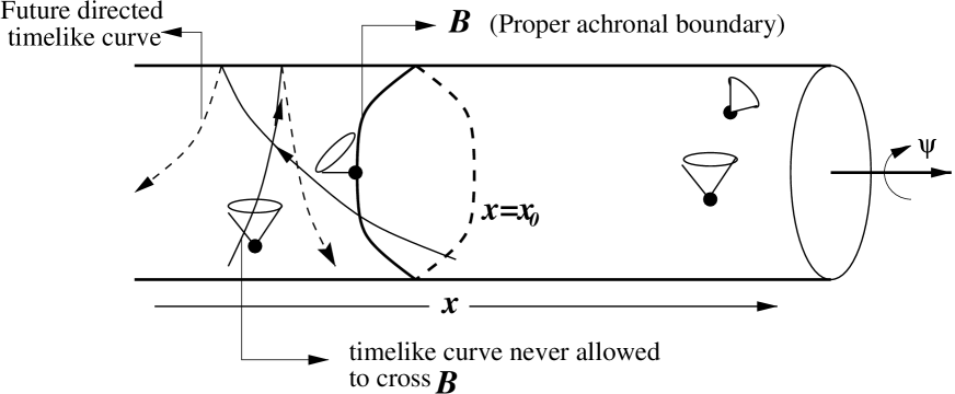
Figure 7: This is an schematic picture of the spacetime analyzed in Example 11. The shown null curve $x=x_{0}$ is an achronal boundary and the future of any point to the left of $B$ is the region $x<x_{0}$, so that $x<x_{0}$ is a future set. Analogously, $x>x_{0}$ is a past set.

It follows that $V$ has as many proper achronal boundaries as the number of zeros of $g(x)$, which may be finite or infinite countable, and the number of future and past sets is that number plus one. If $g(x)$ has no zeros, then the spacetime is totally vicious. If it has $m$ zeros, then the $m+1$ future sets are nested, in the sense that all the future sets whose achronal boundary is $x=x_{j}$ are proper subsets of the future sets whose achronal boundary is $x=x_{i}$ with $x_{j}<x_{i}$.

According to corollary 5.3, any spacetime with a finite number of achronal boundaries (or future sets), as those shown in this example, can only be isocausal to spacetimes with exactly the same number of achronal boundaries (or future sets).

5.4 Sufficient conditions for a causal relationship

We have proved the interesting propositions 5.1, 5.2, 5.3, 5.5, 5.6, 5.7, but apart from the first one all the rest provide only necessary conditions for a diffeomorphism to be a causal relation. Now we are going to present the appropriate sufficient conditions by proving partial converses of some of these results. In order to see that these converses cannot be so simple let us start with an illustrative result of how some “natural” sufficient conditions may fail to work. Consider for instance the condition found in proposition 5.2.

Lemma 5.1

Let $\varphi:V\rightarrow W$ be a diffeomorphism with the property $\varphi(I^{+}(p))\subseteq I^{+}(\varphi(p))\ \forall p\in V$. Then, for all timelike future-directed curves $\gamma\subset V$, any two points $x,y\in\varphi(\gamma)$ satisfy $x<<y$ or $y<<x$.

Proof :    Take any future-directed timelike $\gamma\subset V$ and any two points $p,q\in\gamma$, so that $p<<q$. It is clear that if the assumption for $\varphi$ holds, then $\varphi(p)<\!\!<\varphi(q)$.

Still, the conclusion of this lemma does not imply that $\varphi(\gamma)$ is a timelike curve, even though all its points are chronologically related. Explicit examples of the opposite are given by all totally vicious spacetimes $W$, in which all curves (be them causal or not) satisfy the property that $x<<y$ for every pair of its points. And of course there are spacelike curves in $W$.

What we need here to avoid these counterexamples is to require some causal property for the spacetime $W$.

Lemma 5.2

Let $V$ be a future and past distinguishing Lorentzian manifold. Then every curve $\gamma$ satisfying that $p<<q$ or $q<<p$ for all $p,q\in\gamma$ is timelike and causally oriented.

Proof :    Pick up any $p\in\gamma$ and let ${\cal N}_{p}$ be a normal neighbourhood of $p$. As $V$ is future and past distinguishing there is another neighbourhood ${\cal U}_{p}\subset{\cal N}_{p}$ of $p$ such that all causal curves starting at $p$ cut ${\cal U}_{p}$ in a connected set. Choose any $z\in\gamma\cap{\cal U}_{p}$, so that by assumption $z<<p$ or $p<<z$. In the second possibility there is a timelike future-directed segment $\lambda$, with past and future endpoints at $p$ and $z$ respectively, such that $\lambda\cap{\cal U}_{p}$ must be connected. This implies that $\lambda\subset{\cal U}_{p}$ as ${\cal U}_{p}$ is open, hence $\lambda$ is a future-directed timelike segment contained in the normal neighbourhood ${\cal N}_{p}$. And similarly, but past-directed, in the other possibility $z<<p$. As $z$ was arbitrary, such a segment can thus be constructed for all $z\in\gamma\cap{\cal U}_{p}\subset{\cal N}_{p}$, which implies that $\gamma$ is timelike nearby $p$. Covering $\gamma$ with sets of the type $\gamma\cap{\cal U}_{p}$, $p\in\gamma$, the result follows.

Now we can prove an important partial converse to proposition 5.2.

Proposition 5.8

Let $W$ be future and past distinguishing and $\varphi:V\rightarrow W$ a diffeomorphism such that $\varphi(I^{+}(p))\subseteq I^{+}(\varphi(p))\ \forall p\in V$. Then $\varphi$ is a causal relation and, as a consequence, $V$ is also future and past distinguishing.

Proof :    Take any future-directed timelike curve $\gamma\subset V$. From lemma 5.1 we have that $x<<y$ or $y<<x$ for all $x,y\in\varphi(\gamma)$, and then lemma 5.2 implies that $\varphi(\gamma)\subset W$ is a future-directed timelike curve. As $\gamma$ was arbitrary, proposition 5.1 tells us that $\varphi$ is a causal relation, and then theorem 5.1 ensures that $V$ must be distinguishing.

Finally, we can also prove partial converses to propositions 5.6 and 5.7, which are key results in our work. But first we need a simple lemma taken from [31].

Lemma 5.3

If ${\cal B}^{+}$ is a future set then $p\in\overline{{\cal B}^{+}}\Longleftrightarrow I^{+}(p)\subseteq{\cal B}^{+}$.

Proof :    It is well-known that, for any set $\zeta$, $\overline{I^{+}(\zeta)}=\{x\in V:\ I^{+}(x)\subseteq I^{+}(\zeta)\}$, see e.g. point (iv) in proposition 2.15 of [38]. But for a future set $\overline{{\cal B}^{+}}=\overline{I^{+}({\cal B}^{+})}$, from where the result follows.

Theorem 5.2

Let $W$ be future and past distinguishing. Then, a diffeomorphism $\varphi:V\rightarrow W$ is a causal relation if and only if $\varphi^{-1}({\cal B}^{+})$ is a future set for every future set ${\cal B}^{+}\subseteq W$. And similarly for the past.

Proof :    One implication is proposition 5.6. For the converse, take any $p\in V$ and the future set $I^{+}(\varphi(p))$. Due to the assumption, $\varphi^{-1}(I^{+}(\varphi(p)))$ is a future set. Since $\varphi(p)\in\overline{I^{+}(\varphi(p))}$ then $p\in\overline{\varphi^{-1}(I^{+}(\varphi(p)))}$ and according to lemma 5.3 $I^{+}(p)\subseteq\varphi^{-1}(I^{+}(\varphi(p)))$ so that $\varphi(I^{+}(p))\subseteq I^{+}(\varphi(p))$. As this holds for every $p\in V$ and $W$ is distinguishing, proposition 5.8 ensures that $\varphi$ is a causal relation.

Corollary 5.4

Let $W$ be future and past distinguishing. Then, a diffeomorphism $\varphi:V\rightarrow W$ is a causal relation if and only if $\varphi^{-1}({\cal B})$ is an achronal boundary for every achronal boundary ${\cal B}\subset W$.

All in all, the theorems, corollaries and propositions proved in this section 5, together with Propositions 3.1 and 3.2 and Examples 6, 7, 9 and 11, provide a sufficiently long list of causal objects and properties preserved by causal relations. Irrespective of the above comments on the role which, for instance, future/past sets may play in causality theory, the mentioned list gives sufficient examples of nontrivial causal properties shared by isocausal Lorentzian manifolds from what we conclude that isocausality is actually isolating some essential information about the global causality of the equivalence classes defined by $\sim$. On top of this, as we are going to show in section 6, isocausality is a useful tool in the study of causal boundaries, and allows to generalize and improve the causal diagrams of Penrose type.

6 Causal extensions, causal diagrams and causal boundary of spacetimes

The idea of attaching a causal boundary to a spacetime $V$ was perhaps first developed by Penrose [27, 28, 30] who used a conformal embedding of $V$ into a larger Lorentzian manifold and defined the causal boundary as the boundary of the embedded $V$ in the larger manifold. This idea was subsequently refined by Geroch, Kronheimer and Penrose in [12], where a more general construction for such a boundary (which made use of no embedding in principle) was performed with the only aid of the causal structure of the spacetime under investigation—for distinguishing spacetimes. Although the construction in [12] yielded a satisfactory causal boundary for many relevant spacetimes, it presents some difficulties with other, causally worse-behaved, spacetimes. One example is the Taub spacetime for which the causal boundary obtained by this method does not match the knowledge obtainable using more elementary means, see [23]. Moreover, in order for the causal boundary to be a Hausdorff topological space in this construction, one has to provide an identification rule for the points in the boundary. The original identification rule proposed in [12] does not work accurately in full generality, so that some alternative identification rules and topological constructions were tried for spacetimes with good enough causal properties, see [35, 42, 16]. Unfortunately, they eventually turned out to be not as general as it was initially claimed [25, 16]. There are several other different ways of constructing a boundary (not necessarily “causal”) for Lorentzian manifolds, see [11, 36, 3, 26, 37]. Almost all of them have failed to give a boundary with adequate topological properties for some examples [13, 24, 16]. This has led some researchers to the opinion that not every distinguishing spacetime possesses a proper boundary.

Nevertheless, we would like to contribute to the subject with a new try which is a useful complement to the previous ones and may be helpful in several situations, although perhaps it does not solve all the difficulties just mentioned. As we have already shown, causal relationship generalizes —and in many cases is more useful and manageable than— the conformal relationship. Given that the Penrose conformal diagrams are based on conformal relations, we can try to generalize Penrose’s ideas by using causal relations. In this way we try, on one hand, to attach causal boundaries to general spacetimes, and on the other, to get some intuition and understanding of complicated spacetimes by analyzing the simpler ones to which they are isocausal.

To achieve these goals, we first of all need to include our spacetime $V$ in a larger one (such that the former has a boundary in the latter) but keeping the causal structure of $V$. We do this as follows (compare [37] and definition 3.1 in [38]).

Definition 6.1

An envelopment of $V$ is an embedding $\Phi:V\rightarrow\tilde{V}$ into another connected manifold $\tilde{V}$ with $\Phi(V)\subset\tilde{V}$. A causal extension of $V$ is any envelopment into another Lorentzian manifold $\tilde{V}$ such that $V\sim\Phi(V)$.

Observe that, as is clear, a causal extension for $V$ is in fact a causal extension for coset$(V)$, that is, for all $W$ such that $W\sim V$. It must be remarked that the causal extension is different from the usual extensions in which the (conformal) metric properties of $V$ are kept. Here we only care about the causal structure of $V$, in the sense of definition 5.2, which is at a more basic level. Nevertheless, as is clear any metric or conformal extension is in particular also a causal extension. Of course, as is always the case with extensions, the general causal extensions are not unique, but this is irrelevant for our purposes. Notice that any conformal embedding is in fact a causal extension of the type defined above with the particular choice that the causal equivalence between $V$ and $\Phi(V)$ is of conformal type. We drop here this condition and thereby we generalize the conformal diagrams. The more general diagrams constructed by means of causal extensions will be called causal diagrams.

Example 12

We saw in Example 3 that flat spacetime $\mathbb{L}$ and the static region of de Sitter spacetime $\frac{1}{4}d\mathbb{S}$ are causally equivalent: $\mathbb{L}\sim\frac{1}{4}d\mathbb{S}$. Similarly, we proved in Example 4 that $\mathbb{R}\mathbb{W}_{0}\{\frac{3-n}{n-1}\}\sim\mathbb{L}$. It is completely obvious that the whole de Sitter spacetime $d\mathbb{S}$ is a causal extension of $\frac{1}{4}d\mathbb{S}$, hence $d\mathbb{S}$ is a causal extension also for $\mathbb{L}$ and $\mathbb{R}\mathbb{W}_{0}\{\frac{3-n}{n-1}\}$. Actually, $d\mathbb{S}$ is a causal extension for coset$(\mathbb{L})$. Note that flat spacetime $\mathbb{L}$ is geodesically complete and therefore is not extendible in the usual metric way, but it is certainly extendible in the causal (including the conformal) way.

With this causal extension for $\mathbb{L}$, all members of coset$(\mathbb{L})$ have a boundary when seen as submanifolds of $d\mathbb{S}$. This boundary has a shape of type “$>$”, and it is formed by two null components, and one corner which is a $(n-2)$-sphere (the upper and lower corners are not part of $d\mathbb{S}$ and therefore they are not part of the boundary), see figures 1, 2 and 3(c). They correspond, respectively, to the horizon ($r\rightarrow\alpha$) of $\frac{1}{4}d\mathbb{S}$; to the spacelike and future null infinity and the past singularity in $\mathbb{R}\mathbb{W}_{0}\{\frac{3-n}{n-1}\}$; and to the spacelike and null infinity of $\mathbb{L}$. This is illuminating in three respects:

• firstly, because this boundary for coset$(\mathbb{L})$ does not distinguish between singularities, infinities or removable singularities. It only provides a shape and a causal character for the boundary. This is due to the fact that the specific metric properties have been dismissed. However, one can still recover the distinction between these types of boundaries by including endless curves as will be shown in subsection 6.1.

• secondly, because the boundary found in a given causal extension may not be what one expects to be the entire boundary of a given spacetime. In this particular example, we can also perform another causal extension which includes the upper and lower corners as part of the boundary, i.e. future and past timelike infinity for $\mathbb{L}$, as for instance the typical conformal embedding of $\mathbb{L}$ into the Einstein universe $\mathbb{E}$ which is used traditionally to construct the Penrose conformal diagram of $\mathbb{L}$ [18, 27, 30]. Observe that then spacelike infinity becomes a point, while in the causal extension to $d\mathbb{S}$ it is a $(n-2)$-sphere. This last possibility may be related to the ideas developed by Friedrich in his treatment of conformal field equations near the intersection of null and spacelike infinity, see e.g. [8] and references therein.

• and thirdly, because the boundary built in some particular causal extensions may have different properties than those of other causal extensions, and they may even fail to have some reasonable or desirable features. For instance, it is well known that $\frac{1}{4}d\mathbb{S}$ is conformal to the region $T<-R$ of $\mathbb{L}$ (just take $T=-\alpha e^{-t/\alpha}/\sqrt{1-r^{2}/\alpha^{2}}$, $R=re^{-t/\alpha}/\sqrt{1-r^{2}/\alpha^{2}}$ as the conformal mapping), so that a complete causal boundary for $\frac{1}{4}d\mathbb{S}$, and therefore for $\mathbb{L}$ itself, can be seen as the union of the null hypersurface $T=-R$ with the corresponding part of past null infinity. The trouble here is that this boundary is clearly distinct from the usual boundary obtained by the conformal embedding of $\mathbb{L}$ into $\mathbb{E}$. In the latter, $I^{+}(p\in{\cal J}^{-})$ contains all of ${\cal J}^{+}$ except for part of one null generator, something which is untrue for the former.

Clearly, all this proves on one hand that the causal boundaries found by these means are not unique nor with univocal properties, and on the other that some of them might be more complete, and more appropriate, causal boundaries than others. As a matter of fact, this is a circumstance also shared by the conformal boundary or GKP constructions. We refer the reader to the papers by Harris [15, 16] where the general properties of “reasonable” causal boundary constructions for spacetimes admitting a GKP causal boundary, as well as its possible universality, is considered. We will come back to this point later.

Despite all the problems mentioned in the previous discussion, we put forward the following definition of causal boundary for Lorentzian manifolds based on the idea of isocausality.

Definition 6.2

Let $\tilde{V}$ be a causal extension of $V$ and $\partial V$ the boundary of $\Phi(V)$ in $\tilde{V}$. Then, $\partial V$ is called the causal boundary of $V$ with respect to $\tilde{V}$. A causal boundary is said to be complete if $\Phi(V)$ has compact closure in $\tilde{V}$.

Note that all the members in coset$(V)$ have the same causal boundary with respect to a given causal extension. In principle, however, the causal boundaries of coset$(V)$ depend on its causal extensions. Moreover, the causal boundary may be empty.

Proposition 6.1

If $V$ is compact, then its unique causal boundary is empty.

Proof :    A compact spacetime has no envelopment, because $\Phi(V)$ cannot be a connected compact open proper subset of any $\tilde{V}$.

Of course, all compact spacetimes fail to be chronological [1, 18, 38], and so they are of little physical interest. It seems then reasonable to assume that $V$ is distinguishing in order to attach a causal boundary to $V$. Nevertheless, the causal boundary can still be formed by discrete points (this is what one expects for the boundary of $\mathbb{E}$, see figure 4), or be a set of any co-dimension in $\tilde{V}$. It does not have to be connected either, as the de Sitter spacetime $d\mathbb{S}$ shows. Despite all that, it appears to be natural that the causal properties of, at least, the complete causal boundaries of coset$(V)$ for distinguishing $V$ will be in some sense the same, even though, as remarked before, there may be several different complete causal boundaries!

As we see, our proposal is just a refinement of the original Penrose’s ideas –mixed with some inspiration coming from the abstract boundary construction of [37]– by dropping the conformal property of the embedding: we only require that the embedding be causal. Therefore, our definition covers all the usual cases (such as Penrose’s conformal embeddings and diagrams) in which the causal boundary is built by means of a conformal embedding, because a conformal relation is just a particular type of causal relation (theorem 4.2). Similarly, the cases properly described by using the versions of [12] which involve embeddings (there are non-embedding GKP constructions, see e.g. section 4 in [16]) should also be covered by our definition due to the fundamental theorem 5.2 as the construction in [12] uses just (irreducible) future and past sets. Our choice of causal embedding is motivated by the fact, supported by the results found in section 5, that isocausality is a general concept keeping some important causal properties of spacetimes. Thus, it seems sensible that if one wishes to maintain those causal properties of the original Lorentzian manifold untouched, but without keeping the whole conformal structure, the general way of achieving this goal is by using the isocausality concept.

We cannot claim at this stage that we have succeeded in attaching a causal boundary to spacetimes where other techniques have failed, nor that we have improved the situation substantially. Nevertheless, we can certainly attach a causal boundary, proving also some of its relevant properties, to some Lorentzian manifolds in a very simple manner. Perhaps the most noticeable property of our proposal is that the causal boundaries can be built by elementary means and quite easily for many, even complicated, spacetimes. Some explicit relevant cases are presented in the next examples, including some cases where the Penrose conformal diagram cannot be drawn.

Example 13

In this example we will construct a causal boundary for the Schwarzschild spacetime with negative mass. This spacetime is given in standard spherical coordinates by the line element ($-\infty<t<\infty,\,r>0,\ n\geq 4$)

$$(\overline{\mathbb{S}},\tilde{{\bf g}}):d\tilde{s}^{2}=\left(1+\frac{2M}{r^{n-3}}\right)dt^{2}-\left(1+\frac{2M}{r^{n-3}}\right)^{-1}dr^{2}-r^{2}d\Omega^{2}_{n-2},$$

where $M$ is a positive constant. In order to attach a causal boundary to $\bar{\mathbb{S}}$ we are going to put this spacetime in causal equivalence with another simpler spacetime for which a causal boundary is available. Let us show that flat Minkowski spacetime with a timelike geodesic removed does the job. To that end choose also spherical coordinates for $\mathbb{L}$ and let ($-\infty<T<\infty,\,R>0$)

$$(\mathbb{L}^{*},{\bf g}):ds^{2}=dT^{2}-dR^{2}-R^{2}d{\bar{\Omega}}^{2}_{n-2}.$$

Notice that $\mathbb{L}^{*}$ is $\mathbb{L}$ with the line given by $R=0$ removed. This is in fact the line not covered by the coordinates just introduced, and defines the timelike geodesic previously mentioned. Thus, the base manifold for both $\bar{\mathbb{S}}$ and $\mathbb{L}^{*}$ is simply $\mathbb{R}\times(\mathbb{R}^{n-1}-\{O\})$ being ${O}$ a point of $\mathbb{R}^{n-1}$.

The needed diffeomorphisms are $\varphi:\mathbb{L}^{*}\rightarrow\overline{\mathbb{S}}$ defined simply by $t=T$, $r=R$, and $\psi_{f}:\overline{\mathbb{S}}\rightarrow\mathbb{L}^{*}$ given by $T=bt$, $R=f(r)$ where $b$ is a positive constant and the angular coordinates have been identified as usual. The diagonal form of the tensors $\varphi^{*}\tilde{{\bf g}}$ and $\psi^{*}_{f}{\bf g}$ in appropriate orthonormal bases read

$$\varphi^{*}\tilde{{\bf g}}=\mbox{diag}\left\{\left(1+\frac{2M}{R^{n-3}}\right),-\left(1+\frac{2M}{R^{n-3}}\right)^{-1},\ -1,\dots,-1\right\},$$

$$\psi^{*}_{f}{\bf g}=\mbox{diag}\left\{b^{2}\left(1+\frac{2M}{r^{n-3}}\right)^{-1},-f^{{}^{\prime}}(r)^{2}\left(1+\frac{2M}{r^{n-3}}\right),-\frac{f^{2}(r)}{r^{2}},\dots,-\frac{f^{2}(r)}{r^{2}}\right\}.$$

From this formulae we readily see that $\varphi^{*}\tilde{{\bf g}}$ is a causal tensor for every $R>0$ whereas $\psi^{*}_{f}{\bf g}\in{\cal DP}^{+}_{2}(\overline{\mathbb{S}})$ if the following restrictions are fulfilled

$$b\geq f^{{}^{\prime}}(r)\left(1+\frac{2M}{r^{n-3}}\right),\ b\geq\left(1+\frac{2M}{r^{n-3}}\right)^{\frac{1}{2}}\frac{f(r)}{r}.$$

These are achieved by for instance

$$f(r)=\frac{r^{n-2}}{1+\left(r/M\right)^{n-3}}.$$

Therefore we have proven that $\overline{\mathbb{S}}\sim\mathbb{L}^{*}$ and thus a complete causal boundary for $\mathbb{L}^{*}$ will also be a complete causal boundary for coset$(\mathbb{L}^{*})\ni\overline{\mathbb{S}}$. A possible causal boundary for the former consists on the usual causal boundary of flat spacetime $\mathbb{L}$ plus the removed timelike geodesic. This last line corresponds to the curvature singularity of $\overline{\mathbb{S}}$ located at $r=0$ which, in this particular causal extension, is timelike and represented by a point at each instant of time.

By a similar method one can prove that the inner part of Reissner-Nordström spacetime, the one which contains the singularity and is defined by $r<r_{-}$ (see Example 10), is also isocausal to $\mathbb{L}^{*}$. Thus, the singularity there is also “pointlike” for these causal extensions.

At this stage, we may ask ourselves: how much the previous conclusions depend on the particular causal extension used? It turns out that we can use here the powerful results in [15, 16] to say a word about how the causal boundary would look like for other causal extensions of $\overline{\mathbb{S}}$. Since the GKP construction can be performed explicitly for $\overline{\mathbb{S}}$ as well as for $\mathbb{L}^{*}$ (with a result similar to the one just obtained by our procedure), we can apply the Theorem 3.6 in [16] to ensure that every other causal extension will give a causal boundary with the same chronological properties as the one we have constructed here. This also happens for some other examples in this paper. Thus, the pointlike nature of the singularity in $\overline{\mathbb{S}}$, or in the inner part of Reissner-Nordström spacetime, seems firmly established. Perhaps the advantage of our method lies on its generality and on the elementary means involved in our definition which leads to a much easier and quicker construction than that arising from the GKP definition, which is far more difficult to handle. In summary, it seems clear that the joint use of the GKP construction with our definition in combination with the afore-mentioned results of [16] can provide a very powerful machinery to deal with the causal boundaries of very general spacetimes.

Example 14

In this and the following examples we will construct a causal boundary for some anisotropic but spatially homogeneous “Bianchi-I” spacetimes [22], including the relevant cases of the Kasner Ricci-flat solutions, and the general solution for a comoving dust. All our considerations will be in arbitrary dimension $n$ in these examples, but we have kept the 4-dimensional terminology. This kind of spacetimes has already been used in other causal boundary constructions [11, 16].

The general Bianchi-I Lorentzian manifold, denoted here by $\mathbb{B}_{{\rm I}}$, is characterized by having an Abelian group of motions of $n-1$ parameters acting transitively on spacelike hypersurfaces, the line-element taking the form ($j=1,\dots,n-1$)

$$(\mathbb{B}_{{\rm I}},\tilde{{\bf g}}):d\tilde{s}^{2}=d\bar{t}^{2}-\sum_{j=1}^{n-1}A^{2}_{j}(\bar{t})(d\bar{x}^{j})^{2},\ -\infty<\bar{x}^{j}<\infty$$ (13)

where the $A_{j}(\bar{t})$ are arbitrary functions and the range of the coordinate $\bar{t}$ depends on their particular form. We try to causally compare these spacetimes with the general $n$-dimensional Robertson-Walker geometry with flat slices $\mathbb{R}\mathbb{W}_{0}\{a(t)\}$, already studied in Example 4, and whose line-element in Cartesian-like coordinates takes the form

$$(\mathbb{R}\mathbb{W}_{0}\{a(t)\},{\bf g}):ds^{2}=dt^{2}-a^{2}(t)\sum_{j=1}^{n-1}(dx^{j})^{2},\ -\infty<x^{j}<\infty$$ (14)

where $a(t)$ is the scale factor, which in particular defines the range of the time coordinate $t$. To start with, the diffeomorphism $\varphi_{f}:\mathbb{R}\mathbb{W}_{0}\rightarrow\mathbb{B}_{{\rm I}}$ will be chosen as $(\bar{t},\bar{x}^{j})=(f(t),x^{j})$ where $f$ is a function to be determined. Then, the eigenvalues of $\varphi_{f}^{*}\tilde{{\bf g}}$ with respect to ${\bf g}$ read $\left\{f^{\prime 2}(t),A_{j}(f(t))/a^{2}(t)\right\}$ so that criterion 2 tells us

$$\varphi^{*}\tilde{{\bf g}}\in{\cal DP}^{+}_{2}(\mathbb{R}\mathbb{W}_{0})\Longleftrightarrow a^{2}(t)f^{\prime 2}(t)\geq A^{2}_{j}(f(t)),\,\,j=1,\dots,n-1.$$ (15)

If these relations are fulfilled, then from corollary 3.1 $\mathbb{R}\mathbb{W}_{0}\{a(t)\}\prec\mathbb{B}_{{\rm I}}$. The reciprocal diffeomorphism $\psi_{\bar{f}}:\mathbb{B}_{{\rm I}}\rightarrow\mathbb{R}\mathbb{W}_{0}$ will be taken as $(t,x^{j})=(\bar{f}(\bar{t}),\bar{x}^{j})$. The eigenvalues of $\psi^{*}_{\bar{f}}{\bf g}$ with respect to $\tilde{{\bf g}}$ are

$$\left\{\bar{f}^{\prime 2}(\bar{t}),\frac{a^{2}(\bar{f}(\bar{t}))}{A_{j}^{2}(\bar{t})}\right\}$$

so that again criterion 2 provides

$$\psi_{\bar{f}}^{*}{\bf g}\in{\cal DP}^{+}_{2}(\mathbb{B}_{{\rm I}})\Longleftrightarrow\frac{\bar{f}^{\prime 2}(\bar{t})}{a^{2}(\bar{f}(\bar{t}))}\geq\frac{1}{A^{2}_{j}(\bar{t})},\,\,j=1,\dots,n-1.$$ (16)

If (16) are complied, then $\mathbb{B}_{{\rm I}}\prec\mathbb{R}\mathbb{W}_{0}\{a(t)\}$ from corollary 3.1. When both (15) and (16) are satisfied, then $\mathbb{B}_{{\rm I}}\sim\mathbb{R}\mathbb{W}_{0}\{a(t)\}$. Of course, these are not the only possibilities that make the causal relationship between $\mathbb{B}_{{\rm I}}$ and $\mathbb{R}\mathbb{W}_{0}$ possible, as we have just tried some very particular diffeomorphisms, but they will be enough to prove the causal equivalence of some important subcases of the Bianchi-I spacetimes with the simpler and easier to handle Robertson-Walker Lorentzian manifolds.

Let us start by restricting the $\mathbb{B}_{{\rm I}}$ to be a generalized Kasner spacetime, denoted by $\mathbb{K}\{p_{j}\}$ and defined by $A_{j}(\bar{t})=\bar{t}^{p_{j}}$ for some constants $p_{j}$ (called the Kasner exponents), and $\bar{t}\in(0,\infty)$. The condition (15) is fulfilled if we choose $f(t)=e^{t}$ (with $-\infty<t<\infty$) and $a(t)=B+e^{-kt},\ k=\mbox{max}\{1-p_{j}\},\ B>1$ whenever all the $p_{j}$ are such that $p_{j}\leq 1$. To establish the causal equivalence in this case, it only remains to find an $\bar{f}$ such that (16) holds too. For instance, the function $h(\bar{t})=\frac{Q}{1+\log^{2}\bar{t}}+\bar{t}^{q}$ satisfies $h(\bar{t})\geq\bar{t}^{1-p_{j}}$ for all $\bar{t}\in(0,\infty)$ if $q=\mbox{max}\{1-p_{j}\}>0$ and $Q\geq 1$. Thus, the solution of the differential equation

$$\frac{\bar{f}^{{}^{\prime}}(\bar{t})}{a(\bar{f}(\bar{t}))}=\frac{1}{\bar{t}}\left(\frac{Q}{1+\log^{2}\bar{t}}+\bar{t}^{q}\right)$$ (17)

will provide the required $\bar{f}$. This equation can be solved and the general solution reads

$$\bar{f}(\bar{t})=\frac{1}{k}\log\left\{\frac{1}{B}\left[A\exp\left[kB\left(Q\arctan(\log\bar{t})+\frac{\bar{t}^{q}}{q}\right)\right]-1\right]\right\},$$

where $A$ is an integration constant which must be arranged in such a way that the image of $\bar{f}(\bar{t})$ for $\bar{t}\in(0,\infty)$ covers the whole real line. This is accomplished by taking $A=e^{\frac{kBQ\pi}{2}}$.

Thus, we have proved that $\mathbb{K}\{p_{j}<1\}\sim\mathbb{R}\mathbb{W}_{0}\{B+e^{-kt}\}$ if $k=\mbox{max}\{1-p_{j}\},\ B>1$. This case includes the proper Kasner spacetimes, which are the particular cases with

$$\sum_{j=1}^{n-1}p_{j}=\sum_{j=1}^{n-1}p_{j}^{2}=1,$$ (18)

and then the manifolds are Ricci flat (i.e., solutions of the vacuum Einstein field equations.) From the constraints (18) we clearly have $|p_{j}|\leq 1$ so that if any of the $p_{j}$ is one then the rest of the $p_{j}$ must vanish. This particular simple spacetime with $p_{1}=1$ and $p_{k}=0$ ($k=2,\dots,n-1$) will be dealt with presently as a particular subcase of the general case with $p_{1}=1$, see Example 16.

Once the causal equivalence has been established, we can work with the easier and simpler $\mathbb{R}\mathbb{W}_{0}\{B+e^{-kt}\}$ and try to attach a causal boundary to the class coset$(\mathbb{K}\{p_{j}<1\})$ by attaching it to $\mathbb{R}\mathbb{W}_{0}\{B+e^{-kt}\}\in$ coset$(\mathbb{K}\{p_{j}<1\})$. This is a rather simple task since, for instance, $\mathbb{R}\mathbb{W}_{0}\{B+e^{-kt}\}$ can be written in explicitly conformally flat form by means of the coordinate transformation $\tau=\frac{1}{kB}\log(1+Be^{kt})$

$$ds^{2}=\frac{B^{2}e^{2kB\tau}}{(e^{kB\tau}-1)^{2}}(d\tau^{2}-\sum_{j=1}^{n-1}(dx^{j})^{2}),$$ (19)

where $\tau\in(0,\infty)$. In consequence, the whole flat spacetime $\mathbb{L}$ (for $\tau\in(-\infty,\infty)$) is clearly a causal extension of $\mathbb{R}\mathbb{W}_{0}\{B+e^{-kt}\}$ according to definition 6.1, and then $d\mathbb{S}$ or $\mathbb{E}$ are yet larger causal extensions. From this we deduce that a causal boundary for coset$(\mathbb{K}\{p_{j}<1\})$ is the hypersurface constituted by one spacelike component (the hypersurface $\Sigma$ given by $\tau=0$) representing the past singularity, one null component which represents the null infinity ${\cal J}^{+}$ of flat spacetime, their intersection at $i^{0}$ and the point ${\it i}^{+}$, which correspond respectively to the spacelike and future timelike infinity of Minkowski spacetime. This was to be expected and can be represented in the schematical causal diagram of figure 8-(a). Notice that this contradicts a result found in [16] (p.598), but it seems that correct application of Proposition 5.2 in that paper would lead to the same conclusion as ours.

Figure 8: These are the causal diagrams for the Kasner-type spacetimes. A 3-dimensional version could also be easily drawn by letting these figures become surfaces of revolution around their vertical left ends. We specifically show the causal boundary for Kasner vacuum spacetimes in figure (a) and for the anisotropic Bianchi I dust models (figure (a) if $p_{j}<1$ and figure (b) if $p_{j}>1$). We see that in each case the causal boundary has two components of different causal character, and that the singularity is of null type in the second case.

If on the other hand we assume that every Kasner exponent $p_{j}$ is greater than one, then in the very same way we can prove that $\mathbb{K}\{p_{j}>1\}$ is isocausal with the spacetime with line-element (19) where now $-\infty<\tau<0$. Thus we get for this spacetime the diagram of figure 8-(a) but turned upside-down, with the roles of future and past interchanged. The null component of the causal boundary corresponds now to the singularity and the spacelike component to future infinity, in a behaviour analogous to that of $\mathbb{R}\mathbb{W}\{\gamma\in(-1,\frac{3-n}{n-1})\}$ shown in figure 3 (b). Compare with [16].

Example 15

It is interesting to repeat the previous calculations for the $\mathbb{B}_{{\rm I}}$ model with $A_{j}(\bar{t})=\bar{t}^{p_{j}}(\bar{t}+t_{0})^{\frac{2}{3}-p_{j}}$, $\bar{t}\in(0,\infty)$, where $t_{0}$ a positive constant. This spacetime has physical interest as it provides (in $n=4$) the general solution of Einstein’s equations for Bianchi-I pressure-free perfect fluids whenever the conditions (18) are assumed. We will nonetheless allow for other values of the $p_{j}$. For instance, assume that all the exponents are such that $p_{j}>1$. The conditions (15) hold then if, for example, $f(t)=e^{t}$ and $a(t)=A/\cosh\mu t$ for several suitable choices of the positive constants $A$ and $\mu$. Similarly, conditions (16) are then satisfied by choosing $f(\bar{t})=B\log\bar{t}$ for some suitable $B$ and rearranging, if needed, $A$ and $\mu$ in order to comply with all the inequalities. Thus, these $\mathbb{B}_{{\rm I}}$ models are isocausal to $\mathbb{R}\mathbb{W}_{0}\{\frac{A}{\cosh\mu t}\}$ which may be rewritten in an explicitly conformally flat form by means of the coordinate change $\cosh(\mu t)\,dt=Ad\tau$, leading to

$$d\tilde{s}^{2}=\frac{A^{2}}{1+\mu^{2}A^{2}\tau^{2}}\left(d\tau^{2}-\sum_{j=1}^{n-1}(dx^{j})^{2}\right),\ -\infty<\tau<\infty.$$

We conclude that these $\mathbb{B}_{{\rm I}}$ spacetimes are isocausal to $\mathbb{L}$ and thus we can attach a causal boundary to them similar to that of $\mathbb{L}$, with two null components and three corners, see figure 8 (b). The singularity turns out to be null again, and the future infinity is now of Minkowskian type, with a null component and a point. This is similar to the behaviour of $\mathbb{R}\mathbb{W}_{0}\{\frac{3-n}{n-1}\}$ shown in figure 3 (c).

If all the exponents are lower than one, it is easy to check that the $f(t)=e^{t}$ and the scale factor $a(t)=Q_{1}+e^{-\alpha t}$ for some adequate $Q_{1}$ and $\alpha$ provide an isocausal $\mathbb{R}\mathbb{W}_{0}$ spacetime. The causal boundary in this case, which is the one of physical relevance in $n=4$, turns out to be equivalent to that of Ricci-flat Kasner spacetime, figure 8 (a).

Example 16

In our study of the causal boundary of $\mathbb{K}\{p_{j}\}$ we have restricted ourselves to the situation in which all the exponents are either greater, or lower, than one. It is not difficult to see that the techniques used in the Example 14 do not work for the mixed case with some $p_{i}\geq 1$ and some other $p_{j}\leq 1$ since the diffeomorphisms constructed there fail to be causal relations for the whole Lorentzian manifolds. Now we are going to prove that $\mathbb{K}\{p_{1}=1,p_{k}<1\}$ ($k=2,\dots,n-1$) is isocausal with a precise subregion of flat Minkowski spacetime, and thereby we are going to construct the causal boundary for these spacetimes. The computations work also for the case of $\mathbb{K}\{p_{1}=1,p_{k}>1\}$ with slight changes and a different region of $\mathbb{L}$.

To illustrate why one should expect a more complex causal boundary for these cases, and to get an idea of which type of causal boundary, consider first the extreme case $p_{1}=1$ such that (18) hold. Then, the rest of the exponents vanish and therefore we have

$$p_{1}=1,\ p_{k}=0,\ \,\,\forall\ k=2,\dots,n-1.$$

As is well-known, this special Kasner spacetime $\mathbb{K}\{p_{1}=1,p_{k}=0\}$ is just a region of flat spacetime $\mathbb{L}$. To see it, simply perform the coordinate change $\{\bar{t},\bar{x}^{j}\}\rightarrow\{x^{\alpha}\}$ defined by $x^{0}=\bar{t}\cosh\bar{x}^{1}$, $x^{1}=\bar{t}\sinh\bar{x}^{1}$, and $x^{k}=\bar{x}^{k}$ for $k=2,\dots,n-1$. This change is well-defined for $x^{0}>|x^{1}|$ and the line-element takes the manifestly flat form

$$\left(\mathbb{L}_{+},{\bf g}\right)\,:\,\,\,\,ds^{2}=(dx^{0})^{2}-\sum_{j=1}^{n-1}(dx^{j})^{2},\hskip 28.45274ptx^{0}>|x^{1}|\,.$$ (20)

From now on, we are going to call $\mathbb{L}_{+}$ the region of flat spacetime defined by $x^{0}>|x^{1}|$ (see figure 9). Hence, we have proved that $\mathbb{K}\{p_{1}=1,p_{k}=0\}=\mathbb{L}_{+}$. In particular this means that the whole flat spacetime $\mathbb{L}$, and its causal extensions, are causal extensions for $\mathbb{K}\{p_{1}=1,p_{k}=0\}$ so that a complete causal boundary for $\mathbb{K}\{p_{1}=1,p_{k}=0\}$ has now two null components to the past given by $0<x^{0}=\pm x^{1}$, a corner at their intersection, plus other null component to the future, corners at the intersection of this with the previous ones, and the corner at timelike infinity of $\mathbb{L}$. This is a little bit more complicated structure, and we claim that this is the type of boundary that other $\mathbb{K}\{p_{1}=1,p_{k}<1\}$ will have.

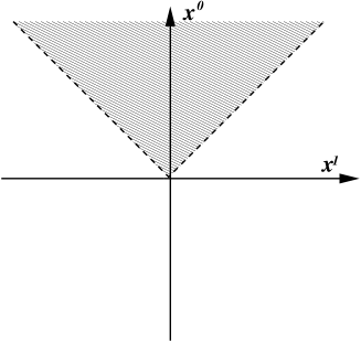
Figure 9: The shaded region of this picture represents the spacetime $\mathbb{L}_{+}$. We appreciate clearly that this is a submanifold of the full Minkowski spacetime $\mathbb{L}$ which metrically extends $\mathbb{L}_{+}$. In a rather similar way the picture for $\mathbb{L}_{-}$ is obtained from this figure by just turning it upside-down (region $x^{0}<-|x^{1}|$).

Bearing this goal in mind, we are going to prove that, in fact, $\mathbb{K}\{p_{1}=1,p_{k}<1\}\in$ coset$(\mathbb{L}_{+})$. Consider first the diffeomorphisms $\psi_{f}:\mathbb{K}\{p_{1}=1,p_{k}<1\}\rightarrow\mathbb{L}_{+}$ defined by

$$x^{0}=f(\bar{t})\cosh(a\bar{x}),\,\,\,x^{1}=f(\bar{t})\sinh(a\bar{x}),\,\,\,x^{k}=\bar{x}^{k}.$$

Then, the eigenvalues of $\psi^{*}_{f}{\bf g}$ with respect to $\tilde{{\bf g}}$ are $\{f^{\prime 2},a^{2}f^{2}/\bar{t}^{2},1/\bar{t}^{2p_{k}}\}$ so that we have

$$\psi^{*}_{f}{\bf g}\in{\cal DP}_{2}^{+}(\mathbb{K}\{p_{1}=1,p_{k}\})\Longleftrightarrow f^{{}^{\prime}}(\bar{t})\geq\frac{a\,|f(\bar{t})|}{\bar{t}},\ f^{{}^{\prime}}(\bar{t})\geq\frac{1}{\bar{t}^{p_{k}}}.$$

Hence, for instance every non-decreasing solution of the differential equation

$$f^{{}^{\prime}}=\frac{a}{\bar{t}}f+\sum_{k=2}^{n-1}\bar{t}^{-p_{k}}$$

will comply with the previous conditions. The general solution of this differential equation is given by ($C$ is an arbitrary integration constant)

$$f(\bar{t})=C\bar{t}^{a}+\sum_{k=2}^{n-1}\frac{\bar{t}^{1-p_{k}}}{1-p_{k}-a}$$

which is easily seen to define a true diffeomorphism $\psi_{f}$ as long as $0<a<$ min$(1-p_{k})$.

For the converse causal relation, let $t$ denote $\sqrt{(x^{0})^{2}-(x^{1})^{2}}$ and choose a diffeomorphism $\varphi_{h}:\mathbb{L}_{+}\rightarrow\mathbb{K}\{p_{1}=1,p_{k}\}$ of type

$$\bar{t}=h(t),\,\,\bar{x}=\frac{b}{2}\log\left(\frac{x^{0}+x^{1}}{x^{0}-x^{1}}\right),\,\,\,\bar{x}^{k}=x^{k}.$$

In this case, if one computes $\varphi_{h}^{*}\tilde{{\bf g}}$ there appear crossed terms in the given coordinates, however by considering the following orthonormal basis in $\mathbb{L}_{+}$

$$\left\{\frac{1}{t}(x^{0}dx^{0}-x^{1}dx^{1}),\frac{1}{t}(x^{1}dx^{0}-x^{0}dx^{1}),dx^{k}\right\}$$

it is easily seen that the eigenvalues of $\varphi^{*}_{h}\tilde{{\bf g}}$ with respect to ${\bf g}$ are given by $\{h^{\prime 2},b^{2}h^{2}/t^{2},h^{2p_{k}}\}$ so that

$$\varphi^{*}_{h}\tilde{{\bf g}}\in{\cal DP}_{2}^{+}(\mathbb{L}_{+})\,\Longleftrightarrow\,h^{\prime}\geq\frac{|h|b}{t},\ h^{\prime}\geq h^{p_{k}}.$$

A possible function $h$ satisfying the previous requirements is given by $h(t)=At^{c}+Bt^{d}$ for appropriate values of $A$ and $B$ as long as the parameters $c$ and $d$ obey

$$c\geq\mbox{max}\left\{\frac{1}{1-p_{k}}\right\}\geq\mbox{min}\left\{\frac{1}{1-p_{k}}\right\}\geq d\geq b>1.$$

Under these assumptions, $h(t)$ is a diffeomorphism of $\mathbb{R}^{+}$ into itself from what we finally obtain the desired result $\mathbb{L}_{+}\sim\mathbb{K}\{p_{1}=1,p_{k}<1\}$. Thus, with the causal equivalence just constructed, the causal diagram for $\mathbb{K}\{p_{1}=1,p_{k}<1\}$ can be easily constructed, and we can also attach a complete causal boundary to them, which is the causal boundary of coset$(\mathbb{L}_{+})$ previously mentioned. This is shown in figure 10.

Figure 10: This is the causal diagram for all Kasner-like spacetimes with $p_{1}=1$ and $p_{k}<1$. The spacetime is the part above the singularity and below the future infinity ${\cal J}^{+}$. As we see, a 3-dimensional figure is needed here to account for the basic properties of the causal boundary. The past singularity is of null type with two branches. The spacetime has no past particle horizon in the direction defined by the null generator of this singularity. However, there are past particle horizons in every other direction. The future infinity has the usual structure of Minkowski spacetime. In the case $p_{k}>1$, the causal diagram is the one shown here but turned upside down, with the roles of the singularity and infinity interchanged, so that the singularity is also in the past and now there are future particle horizons, but no past ones.

Similarly, one can prove along the same lines that $\mathbb{K}\{p_{1}=1,p_{k}>1\}\in$ coset$(\mathbb{L}_{-})$ where now $\mathbb{L}_{-}$ is the region of flat spacetime defined by $x^{0}<-|x^{1}|$ (see figure 9). In this case the causal diagram is the time reversal of that in figure 10, but now of course with the roles of the singularity and infinity interchanged so that the singularity is still in the past.

6.1 Identifying the parts of a causal boundary

We can use the ideas developed so far to try to identify the various parts of a causal boundary. As we have seen, the causal boundaries can be endowed with causal properties (we can say if they have null components, or spacelike ones, etc), but we are not able to say if these components are part of the singularity, or of infinity. To do that, of course, we must use at least part of the metric properties of $V$: essentially those characterizing the completeness or not of causal curves (see e.g. [18, 44, 38] for the definition of completeness). Namely

Definition 6.3

Let $\partial V$ be the causal boundary of $V$ with respect to the causal extension $\tilde{V}$. A point $\tilde{p}\in\partial V$ is said to belong to:

1. a singularity set ${\cal S}\subseteq\partial V$ if it is the endpoint in $\tilde{V}$ of a curve which is endless and incomplete within $V$.

2. future infinity ${\cal J^{+}}\subseteq\partial V$ if it is the endpoint in $\tilde{V}$ of a causal curve which is complete to the future in $V$. And similarly for the past infinity ${\cal J^{-}}$.

3. spacelike infinity $i^{0}\subseteq\partial V$ if it is the endpoint in $\tilde{V}$ of a spacelike curve which is complete in $V$.

The unions of all past and future infinities will be also termed as causal infinity. In principle, there is no reason to believe that all points in a causal boundary belong to one of the possibilities of the previous definition, nor that the different possibilities are disjoint in general.

Example 17

Coming back to the Example 12, where we saw that $d\mathbb{S}$ was a causal extension for coset$(\mathbb{L})\supset\left\{\mathbb{L},\frac{1}{4}d\mathbb{S},\mathbb{R}\mathbb{W}_{0}\{\frac{3-n}{n-1}\}\right\}$, we can now easily identify the different parts of the causal boundary. For $\mathbb{L}$, which is b-complete (all curves are complete), the upper (lower) null component of the boundary is future (past) null infinity, and the corner is spacelike infinity. For $\frac{1}{4}d\mathbb{S}$, the whole causal boundary is a singularity. Of course, this is a removable singularity [38], as $\frac{1}{4}d\mathbb{S}$ can be metrically extended to the whole of $d\mathbb{S}$, but this is another matter. Finally, for $\mathbb{R}\mathbb{W}_{0}\{\frac{3-n}{n-1}\}$ the future null component of the causal boundary represents future infinity, the corner is spacelike infinity, and the past null component is the “big-bang” singularity. Note that in this case the singularity is essential (irremovable by metric extensions [38]). A similar behaviour is the one found for the Bianchi-I dust spacetimes in figure 8 (b).

The above considerations allow us to put forward a tentative characterization of causally asymptotically equivalent spacetimes at a level which does not use the whole information contained in the Lorentzian metric. This information might be included in a subsequent step if one wishes to define asymptotically flat, or asymptotically $d\mathbb{S},\ \mathbb{A}d\mathbb{S}$, etc, spacetimes. We are now just caring about the causal properties of the asymptotic structure, only distinguishing between infinities and singularities. The idea is to say that two spacetimes have the same asymptotic properties from the causal point of view if there are arbitrarily small neighbourhoods of the relevant parts of their causal boundaries which are isocausal. To that end, we need to know what is a neighbourhood of a causal boundary and its parts.

Definition 6.4

An open set $\zeta\subset V$ is called a neighbourhood of

1. the causal boundary of $V$ if $\zeta\cap\gamma\neq\emptyset$ for all endless causal curves $\gamma$;

2. a singularity set ${\cal S}$ if $\zeta\cap\gamma\neq\emptyset$ for all endless curves $\gamma$ which are incomplete towards ${\cal S}$;

3. causal (future, past) infinity if $\zeta\cap\gamma\neq\emptyset$ for all complete (complete to the future, to the past) causal curves $\gamma$.

Let us remark that we do not need to use any causal extension in the preceding definition. Only the properties of $V$ are required. Then we introduce the following definition, which might require some refinement.

Definition 6.5

$W$ is said to be causally asymptotically like $V$ if any two neighbourhoods of their causal infinities $\zeta\subset V$ and $\tilde{\zeta}\subset W$ contain corresponding neighbourhoods $\zeta^{\prime}\subset\zeta$ and $\tilde{\zeta}^{\prime}\subset\tilde{\zeta}$ of the causal infinities such that $\zeta^{\prime}\sim\tilde{\zeta}^{\prime}$.

Similar definitions can be given for $W$ having causally the singularity structure of $V$, or the causal boundary of $V$, replacing in the given definition the neighbourhoods of the causal infinity by those of the singularity and of the causal boundary, respectively.

In the previous Example 17, it is easy to see that $\mathbb{R}\mathbb{W}_{0}\{\frac{3-n}{n-1}\}$ is future asymptotically “flat” (that is, future asymptotically equivalent to $\mathbb{L}$) from the causal point of view, while $\frac{1}{4}d\mathbb{S}$ has a past-singularity of the type of $\mathbb{R}\mathbb{W}_{0}\{\frac{3-n}{n-1}\}$ (of course, removable!). A more interesting case arises from Example 9, where we proved that $\mathbb{S}_{a}\sim\mathbb{L}_{a}$ for all $a>c_{M}$. This clearly means, according to definitions 6.4 and 6.5, that the causal infinities for flat and outer Schwarzschild spacetimes are causally equivalent.

7 Conclusions

In this work a new tool for the causal analysis of Lorentzian manifolds has been defined and developed. The most remarkable of its properties are: (i) that the causality constraints are kept in isocausal spacetimes; (ii) the precise relationships between some causal objects—like achronal boundaries, and future/past sets, curves, or tensors–; (iii) the generalization it provides of conformal relations; and (iv) the refinement of the classical causality conditions, which can also be considered in an abstract way. Furthermore, the whole idea allows us to undertake the study of global causal properties of spacetimes with a high degree of generality, for one can get a first impression of the properties of general spacetimes by studying other spacetimes which are simpler but nevertheless isocausal to the former. In particular we can draw causal diagrams, which are clear generalizations of the Penrose conformal diagrams, and obtain causal boundaries for general spacetimes by using quite simple and elementary means.

Several questions remain open, as for example the need for improvements and some general results on the criteria used to discard or to prove the possible causal relation between given spacetimes, the existence of upper and lower bounds for causally ordered sequences of equivalence classes of isocausal spacetimes, the precise extent to which isocausal spacetimes can be thought of as sharing the same causal properties, and the intrinsic or uniqueness properties of the different causal boundaries constructed by means of causal extensions, among others.

References

References

- [1] Beem J K, Ehrlich P E, and Easley K L 1996 Global Lorentzian Geometry (Pure and Applied Math. 202, Marcel Dekker, New York)
- [2] Bergqvist G and Senovilla J M M 2001 Class. Quantum Grav. 17 2799
- [3] Budic R and Sachs R K 1974 J. Math Phys. 15 1302
- [4] Carter B 1971 Gen. Rel. Grav. 1 349
- [5] Choquet-Bruhat Y and Geroch R P 1969 Commun. Math. Phys. 14 329
- [6] See e. g. Dugundji 1966 Topology (Allyn and Bacon Inc., Boston) p. 96
- [7] Eisenhart L P 1949 Riemannian Geometry (Princeton Univ. Press, Princeton)
- [8] Friedrich H 1998 J. Geom. Phys. 24 83
- [9] García-Parrado A and Senovilla J M M 2002, “Causal relations and their applications”, math-ph/0202005.
- [10] García-Parrado A and Senovilla J M M 2002 “Causal symmetries” (under preparation).
- [11] Geroch R 1968 J. Math. Phys 9 450
- [12] Geroch R, Kronheimer E H and Penrose R 1972 Proc. R. Soc. Lond. A 327 545
- [13] Geroch R, can-bin Liang and Wald R 1982 J. Math. Phys. 23 432
- [14] Gödel K 1949, Rev. Mod. Phys. 21 447
- [15] Harris S G 1998, J. Math. Phys. 39 5427
- [16] Harris S G 2000, Class. Quantum Grav. 17 551
- [17] see e. g. Hausdorff F 1978 Set Theory (Chelsea, New York)
- [18] Hawking S W and Ellis G F R 1973 The large scale structure of spacetime. (Cambridge University Press, Cambridge)
- [19] Hawking S W King A R and McCarthy P J 1976 J. Math. Phys. 17 174
- [20] Huang W 1998 J Math. Phys 39 1637
- [21] Hull, C M 1984 Phys. Lett. B139 39; Figueroa-O’Farrill, J M 2000 Class. Quantum Grav. 17 2925; Güven, R 2000 Phys. Lett. 482 255
- [22] Kramer D, Stephani H, MacCallum M A H and Herlt E 1980 Exact Solutions of Einstein’s Field Equations (Cambridge University Press, Cambridge)
- [23] zhi-quan Kuang, jian-zeng Li and can-bin Liang 1986 Phys. Rev. D 33 1533
- [24] zhi-quan Kuang and can-bin Liang 1988 J. Math. Phys. 29 433
- [25] zhi-quan Kuang and can-bin Liang 1992 Phys. Rev. D 46 4253
- [26] Meyer D 1985 J. Math Phys. 27 124
- [27] Penrose R 1963 Phys. Rev. Lett. 10 66
- [28] Penrose R 1964 in Relativity, Groups and Topology C.M. de Witt and B. de Witt eds., les Houches summer school 1963 (Gordon and Breach, New York)
- [29] Penrose R 1965 Rev. Mod. Phys. 37 215
- [30] Penrose R 1968, in Batelle Rencontres C.M. de Witt and J.A. Wheeler, eds. (Benjamin, New York)
- [31] Penrose R 1972 Techniques of Differential Topology in Relativity. (Regional Conference Series in Applied Math. 7, SIAM Philadelphia)
- [32] Penrose R 1980 “On Schwarzschild Causality” in Essays in General Relativity. A festschrift for A. Taub, F.J.Tipler ed. (Academic Press, New York).
- [33] Pitts J B and Schieve W C 2001 Found. Phys. 31 1083
- [34] Pitts J B and Schieve W C 2001, preprint gr-qc/0111004
- [35] Rácz I 1987, Phys. Rev. D 36 1673; 1988 Gen. Rel. Grav. 20 893
- [36] Schmidt B G 1971 Gen. Rel. Grav. 1 269
- [37] Scott S and Szekeres P 1994 J. Geom. Phys. 13 223
- [38] Senovilla J M M 1998 Gen. Rel. Grav. 30 701
- [39] Senovilla J M M 2000 Class. Quantum Grav. 17 2799
- [40] Senovilla J M M 2002, “Superenergy tensors and their applications”, math-ph/0202029.
- [41] Sorkin R D, Meyer D, Joohan L and Bombelli L 1987 Phys. Rev. Lett. 59 521
- [42] Szabados L B 1988 Class. Quantum Grav. 5 121; 1989 ibid. 6 77
- [43] Tipler F J 1986, J. Math. Phys. 27 559
- [44] Wald, R M 1984 General Relativity (The University of Chicago Press, Chicago)