Numerical evolution of axisymmetric, isolated systems in General Relativity

Abstract

We describe in this article a new code for evolving axisymmetric isolated systems in general relativity. Such systems are described by asymptotically flat space-times which have the property that they admit a conformal extension. We are working directly in the extended ‘conformal’ manifold and solve numerically Friedrich’s conformal field equations, which state that Einstein’s equations hold in the physical space-time. Because of the compactness of the conformal space-time the entire space-time can be calculated on a finite numerical grid. We describe in detail the numerical scheme, especially the treatment of the axisymmetry and the boundary.

I Introduction

Currently, there are three main approaches to solve Einstein’s field equations using numerical methods. They differ in the way they set up systems of equations and the appropriate initial boundary value problems which they try to solve. The main approach is based on variants of the ADM equations Arnowitt et al. (1962) which are written as a hyperbolic system of evolution equations. The IBVP is set up on space-like hypersurfaces with boundary ‘far out’ in a region where it is assumed that the space-time is such that in a certain approximation it is close to the Minkowski or Schwarzschild space-time or a perturbation thereof. Radiation is extracted by matching to such approximate space-times.

The second approach is based on the characteristic initial value problem which is based on outgoing null hypersurfaces. The Einstein equations can be written in this context in a hierarchical form which lends itself very easily to numerical treatment. The use of outgoing null hypersurfaces has the advantage that radiation of any type and, in particular, gravitational radiation can be followed all the way out to an asymptotic observer (LIGO) located at null-infinity. By using a compactified radial coordinate it is possible to read of the radiation at finite points.

There are some attempts to match these two approaches in the so called Cauchy-Characteristic Matching procedure (CCM) where the two schemes exchange appropriate information across an interface to provide boundary conditions at a time-like hypersurface (see Winicour (1998) for a recent review).

The third approach, termed the conformal approach, is somewhat different. While the previous methods set up equations directly for the physical quantities in the physical space-time in this approach one formulates the so called ‘conformal field equations’ for quantities on a conformally related space-time, which state in an indirect way, that the physical Einstein tensor vanishes. This indirection introduces some freedom which is used to compactify the space-time in so that it is possible to hold the entire (semi-global) problem on a finite grid. In this way one can solve a global problem with finite resources. Since the whole space-time is accessible one can also read off radition without further approximation. Due to these properties the conformal approach is well suited to study global properties of space-times.

All these approaches have certain more or less severe draw-backs. Common to all of them is the fact that the constraints which can be satisfied initially very accurately are violated during the course of the evolution and this ‘constraint violation’ seems to grow in all codes with an exponential rate.

The standard Cauchy approach suffers from the fact that the outer boundary is very difficult to handle. This is due to a lack of understanding of the appropriate IBVP in the sense that there is no boundary condition known, which would be physically meaningful (modelling the fact that the space-time should be asymptotically flat) as well as numerically stable. The characteristic codes crash when the underlying outgoing null hypersurfaces form caustics and self intersections. In the conformal approach there are no (known) difficulties out of principle. The problems arising there as we will point out in this work (see also a recent discussion in Frauendiener (2002)) are of a numerical nature or due to the complexity of the equations.

The conformal approach has been pioneered by Hübner who implemented the first code treating a spherically symmetric space-time with a scalar field coupled to gravity Hübner (1994). He also succeeded to evolve general initial data which were close enough to flat data to evolve into a global space-time with a regular $i^{+}$ Hübner (2001) (see also Husa (2002)).

We present in this work a code to solve the conformal field equations for space-times which are axisymmetric with a regular axis. In contrast to previous work Frauendiener (1998a, b, 1999) where the unphysical assumption was made that there are no fixed points now we assume the existence of a regular axis which implies that we can now treat physically relevant isolated systems.

Our motivation for developing a 2D instead of a full blown 3D code is that we want to have a code with reasonable turn around times that allows us to study the effects of changing various properties such as gauges, boundary conditions etc. within a reasonable time. Futhermore, in contrast to a 3D code a 2D code allows us to compute the space-times with a much higher resolution.

The plan of this paper is as follows. In sec. II we review the basics of the conformal approach, write down the conformal field equations and discuss the implementattion of the axisymmetry. Sec. III is devoted to the description of the numerical methods used in the code. In particular, we discuss the evolution algorithm, the boundary conditions and the issues arising from the axisymmetry. In sec. IV we present the results obtained so far and conclude with a summary in sec. V.

II The General Setting

II.1 The Conformal Field Equations

In this section we first give a short introduction into the conformal picture and provide the conformal field equations. Then we introduce the hyperboloidal initial value problem for the conformal field equations by making a $3+1$-decomposition with respect to a frame into a system of constraint equations and a system of symmetric hyperbolic evolution equations.

We then describe how to implement the axisymmetry with special emphasis on the regularity of the axis. The symmetry reduces the problem from a 3D to a 2D problem, but does not lead to a significant reduction of components. We therefore assume additionally, that the Killing vector field $\xi^{a}$, which generates the axisymmetry is orthogonal to the hypersurfaces of constant $\phi$, where $\phi$ is the parameter along the orbits of $\xi^{a}$ (i.e., $\xi(\phi)=1$). This gives us an additional discrete symmetry, which reduces the number of components from 65 for the general equations to 35 independent components.

Suppose we have a vacuum solution $(\widetilde{\mathcal{M}},\tilde{g})$ of the Einstein equations, which we will call the ‘physical space-time’. This space-time is asymptotically flat at null-infinity (‘light-like asymptotic flatness’) and hence describes an isolated general relativistic system, if it admits the following construction.

There exists a smooth Lorentz manifold $(\mathcal{M},g_{ab})$ and a diffeomorphism $\Psi:\widetilde{\mathcal{M}}\longrightarrow\mathcal{M}$, such that:

1. $\Psi(\widetilde{\mathcal{M}})\subset\mathcal{M}$ and $\Psi(\widetilde{\mathcal{M}})$ has a smooth boundary, $\partial{\Psi(\widetilde{\mathcal{M}})}=\mbox{ I}$ with $\mbox{ I}=\mbox{ I}^{+}\cup\mbox{ I}^{-}$ and $\mbox{ I}^{+}\cap\mbox{ I}^{-}=\emptyset$.

2. there exists a smooth function $\Omega$ on $\mathcal{M}$, such that: $g_{ab}=\Omega^{2}(\Psi^{-1})^{*}\tilde{g}_{ab}$ and $\Omega\neq 0$ on $\Psi(\widetilde{\mathcal{M}})$,

3. on I the conformal factor $\Omega=0$ and $d\Omega\neq 0$,

4. every null geodesic in $\widetilde{\mathcal{M}}$ has a future endpoint on $\mbox{ I}^{+}$ and a past endpoint on $\mbox{ I}^{-}$,

5. the Ricci tensor $\tilde{R}_{ab}$ of the physical metric $\tilde{g}_{ab}$ vanishes in a neighborhood of I, $\tilde{R}_{ab}=0$.

This construction states, that the physical manifold $(\widetilde{\mathcal{M}},\tilde{g})$ is conformal to the interior of the ‘unphysical’ manifold $(\mathcal{M},g)$. In order to simplify the notation, we will discard further on the diffeomorphism $\Psi$ and identify the points $p\in\widetilde{\mathcal{M}}$ and $\Psi(p)\in\mathcal{M}$. The boundary I of $\widetilde{\mathcal{M}}$ in $\mathcal{M}$ represents ‘infinity’ of the physical manifold. The asymptotic region I is in a sense unique for all asymptotically flat space-times and defines a unique ‘background’ structure, on which one can define the mass of a space-time and the gravitational radiation measured by an observer at infinity.

Since one has immediate access to the geometric structure at I in the unphysical manifold $\mathcal{M}$, it is reasonable to solve the conformally transformed Einstein equations directly in $\mathcal{M}$. Now the problem arises, that the transformed Einstein equations are formally singular at I. This problem was solved by Friedrich Friedrich (1981), who proposed the conformal field equations, a system of regular equations for the geometric structure on $\mathcal{M}$. If there exists a triple $(\mathcal{M},g,\Omega)$ satisfying the conformal field equations then the pair $(\widetilde{\mathcal{M}},\tilde{g})$, where $\widetilde{\mathcal{M}}=\{\Omega>0\}$ and $\tilde{g}=\Omega^{-2}\,g$ is a vacuum space-time.

Let us consider the abstract manifold $\mathcal{M}$ with the additional structure of a metric $g_{ab}$ and a metric compatible connection $\nabla_{a}$. $T^{a}{}_{bc}$ and $R^{a}{}_{bcd}$ are the torsion and curvature tensors, respectively, associated with $\nabla_{a}$. Additional variables are the conformal factor $\Omega$, a 1-form $\Sigma_{a}$, a scalar function $S$, a symmetric traceless tensor field $\Phi_{ab}$ and a completely traceless tensor field $K_{abcd}$ with the symmetries of the Weyl tensor.

Then the conformal field equations read:

$$T^{a}{}_{bc} =0,$$ (1)

$$R_{abcd}-\Omega K_{abcd}+2g_{c[a}\Phi_{b]d}-2g_{d[a}\Phi_{b]c}$$

$$-4g_{c[a}g_{b]d}\Lambda =0,$$ (2)

$$2\nabla_{[c}\Phi_{a]b}+2g_{b[c}\nabla_{a]}\Lambda-K_{cab}{}^{d}\Sigma_{d} =0,$$ (3)

$$\nabla_{a}K^{a}{}_{bcd} =0,$$ (4)

$$\nabla_{a}\Omega-\Sigma_{a} =0,$$ (5)

$$\nabla_{a}\Sigma_{b}-g_{ab}S+\Omega\Phi_{ab} =0,$$ (6)

$$\nabla_{a}S+\Phi_{ab}\Sigma^{b}-\Omega\nabla_{a}\Lambda-2\Lambda\Sigma_{a} =0,$$ (7)

$$2\Omega S-2\Omega^{2}\Lambda-\Sigma_{a}\Sigma^{a} =0.$$ (8)

The first equation states, that the torsion tensor $T^{a}{}_{bc}$ vanishes, so that $\nabla_{a}$ is the Levi-Civita connection of the metric $g_{ab}$ and (II.1) is the decomposition of the curvature tensor into its irreducible parts. Since one can show that the Weyl tensor $C^{a}{}_{bcd}$ necessarily vanishes on I it is written as $C_{abcd}=\Omega K_{abcd}$. $\Phi_{ab}$ is the traceless part of the Ricci tensor and $\Lambda$ is proportional to the Ricci scalar, $R=24\Lambda$. Eq. (5) serves to get first order equations and, therefore, must be regarded as the definition of $\Sigma_{a}$. Eqs. (6) and (8) are the expressions for the conformally transformed traceless part of the physical Ricci tensor and the physical scalar curvature, respectively. Eqs. (3) and (4) are the conformally transformed Bianchi identities of the physical manifold, which form a central part of the conformal field equations.

Now we have to set up an initial value problem for the conformal field equations. We do this by the usual $3+1$-decomposition. Since we are working in the tetrad formalism, we pick a tetrad $e^{a}_{\mu}$ with $g_{ab}=\eta_{\mu\nu}e^{\mu}_{a}\otimes e^{\nu}_{b}$, ($e^{\nu}_{b}$ being the dual frame of covectors) where $t^{a}=e^{a}_{0}$ is orthogonal to the hypersurface $\mathcal{S}$ of constant coordinate time $t$, so the manifold is sliced in the way $\mathcal{M}=\mathbb{R}\times\mathcal{S}$. In a tedious but straightforward procedure we get a system of symmetric hyperbolic evolution equations, together with a system of constraints.

In this process, we also have to fix the gauge freedom. This is done here by adding appropriate equations to the system, which contain four free functions, which determine the coordinates, six free functions corresponding to the freedom in the choice of the tetrad. Since the conformal field equations are invariant under conformal rescalings $\Omega\rightarrow\omega\Omega,g_{ab}\rightarrow\omega^{2}g_{ab}$, where $\omega$ has to be strictly positive, there is one additional function to fix the conformal factor. The details of this hyperbolic reduction together with the fixing of the gauges are described in Friedrich (1996) and Frauendiener (2000).

Since our version of the conformal field equations is not suited to treat space-like infinity $i^{0}$ in an appropriate way (see Friedrich (2002) for a discussion of other formulations of the conformal field equations) we choose as the initial data hypersurface a hyperboloidal slice of $\mathcal{M}$. This hyperboloidal slice intersects $\mbox{ I}^{+}$ in a space-like 2-surface, in contrast to an asymptotically Euclidean hypersurface which reaches spatial infinity $i^{0}$. Since a hyperboloidal slice is not a Cauchy surface for the entire space-time, we are not able to calculate the entire space-time, but we can do semi-global evolutions into the future. This is enough for our purposes, because we are mainly interested in the asymptotic regions near and including I, where we can read off the gravitational radiation emitted within the manifold.

II.2 Axisymmetry

We assume axisymmetry of our physical space-time $\widetilde{\mathcal{M}}$, see Carot (2000) for a definition. The assumption of axisymmetry is motivated by the fact, that we can reduce the numerical problem from a 3D to a 2D problem and that this symmetry still allows gravitational radiation, see Ashtekar and Xanthopoulos (1978) for the symmetries which admit radiation for light-like asymptotically flat space-times. This allows us to simulate interesting radiating systems with high accuracy already on small computers. The symmetry will be transferred to the conformal space-time $\mathcal{M}$, if the conformal factor $\Omega$ is also invariant under the symmetry $\mathcal{L}_{\xi}\Omega=0$, which we assume explicitly by partly using up the gauge freedom in $\Omega$.

The reduction from a 3D to a 2D problem is achieved by evolving only within one of the hypersurfaces of constant $\phi$. All these hypersurfaces are isometric and so it is enough to calculate all fields on one of them. The tricky part of axisymmetric systems is the analytic and numerical treatment of the axis. From the analytical side, one would like to exclude pathological things, like a massive string on the axis. This means we would like to have a space-time, which is regular on the axis. The regularity of the axis is usually ensured by the condition of elementary flatness Carot (2000) on the axis. But this condition is very hard to implement numerically. Fortunately, there is an equivalent condition of Wilson and Clarke in Wilson and Clarke (1996), which simply states, that if the Killing vector $\xi^{a}$ has the same form as in Cartesian coordinates and the metric is differentiable in a neighborhood of the axis, which we have to assume anyway for the numerics, then the axis is regular. This is the reason, why we use Cartesian coordinates in our code. We evolve in the hypersurface, where $\phi=0$, because there the Cartesian $(x,z)$-coordinates coincide with the $(r,z)$-coordinates of polar coordinates. In the following, we will call this hypersurface the ‘evolution hypersurface’.

Apart from the axisymmetry we have an additional discrete symmetry because the Killing vector $\xi^{a}$ is orthogonal to hypersurfaces of constant $\phi$, so the reflection $i$ across the evolution hypersurface given by $\phi\mapsto-\phi$ and hence $\xi^{a}\mapsto-\xi^{a}$ is an isometry. Thus, by adapting the tetrad $e^{a}_{\mu}$ to the Killing vector, i.e., $e^{a}_{3}\sim\xi^{a}$, in the evolution hypersurface we can achieve a reduction of the independent tensor components. For this reduction we have to distinguish between tensors fields, which are invariant under $i$ or which are mapped onto their negative. In the first (second) class all tensor components obtained by contracting with an odd (even) number of $e^{a}_{3}$ will be zero. This reduces the problem from 65 free components to 35 components.

III Numerics

In this section we want to describe the numerical scheme, which we used to solve the conformal field equations. Besides the conformal field equations we tested the same scheme also on the scalar wave equation in the Minkowski space-time. The numerical grid is uniform and rectangular, where the outermost points are used for the boundary. Since we use a non-staggered grid, $x=0$, is one of the boundaries of our grid. All of these points lie on the axis of the space-time, which is not a boundary of the space-time. Therefore, we have to treat these points in a different way, which will be described in the subsection on axisymmetry and the cartoon-method.

III.1 Evolution

For the evolution the Method of Lines is used. This is a semi-discrete method for solving partial differential equations. The PDEs are discretized in space to obtain a system of ODEs which are then integrated in time along the lines in space-time given by fixing the grid points. We use two standard methods for solving the ensuing ODEs: a Runge-Kutta method and the multilevel Adams-Bashforth scheme, both of fourth order in time. In addition, we have used the iterative Crank-Nicholson (ICN) scheme Teukolsky (2000), which is an explicit form of the implicit Crank-Nicholson scheme. These three methods are all explicit, which makes them easy to implement in the code. Nevertheless implicit methods would have better stability properties, but compared to explicit methods they would be much slower, because one has to solve a big system of nonlinear, coupled equations at each time step.

The spatial discretization can be chosen between second order and fourth order central stencils, but we use fourth order discretization in all test runs, as there was no difference in the stability properties of the method, only in the accuracy of the solution obtained.

III.2 Axisymmetry and the Cartoon-Method

We stated in the last chapter, that we use Cartesian coordinates, so that the axis is regular. Despite the fact that we are using non adapted coordinates, we can reduce the problem from 3D to 2D by evolving in the hypersurface, where $\phi=0$ and the Cartesian coordinates $(x,z)$ coincide with the cylindrical coordinates $(r,z)$. The problem, which arises now, is, that we will need derivatives across this evolution hypersurface. We solve this by applying an idea of Alcubierre et al. Alcubierre et al. (1999), which they call the cartoon-method. They have proposed, that instead of using the symmetry in adapted coordinates $\partial_{\phi}T=0$, one can use the symmetry as a tensor equation $\Phi^{*}T=T$ in Cartesian coordinates, where $T$ is an arbitrary axisymmetric tensor. Because of the use of Cartesian coordinates, we get in this way a regular axis and at the same time we avoid the coordinate singularity of adapted coordinates and the resulting singular components at the axis. One could certainly cure the singularities of adapted coordinates by a regularizing procedure for the components and the equations at the axis. But it should be clear, that this change of the equations is a possible source of instabilities and for our large system of 35 independent components, it would have been at least tedious to check the behavior of each component at the axis (see Evans (1985), Thornburg (1996) for such regularization procedures and Garfinkle (2002) for a more recent approach). As Cartesian coordinates are often used in 3D codes, the cartoon method has the additional advantage that we can easily compare the results of our code with that of 3D codes. In the following we give the formulation of the cartoon-method in the tetrad formalism.

Since we are using a tetrad basis we not only have to ensure the regularity of our coordinates, but also the regularity of our tetrad at the axis. Additionally, we have the constraint, that one basis vector $e^{a}_{i}$ has to be orthogonal to the evolution hypersurface, so that we can use the discrete symmetry $i$ to reduce the number of independent components. Apart from these two conditions we can arbitrarily fix the tetrad in our space-time. We first introduce an invariant tetrad $f^{a}_{\mu}$, where $f^{a}_{3}\sim\xi^{a}$ and $\Phi_{*}f^{b}_{\mu}=f^{b}_{\mu}$. Similar to adapted coordinates, this adapted tetrad is singular on the axis. But we have ensured, that our manifold is elementary flat at the axis, so we only have to rotate the tetrad in the neighborhood of the axis, to a tetrad which has a smooth limit while approaching the axis. So we make the ansatz, that the tetrad is given by the rotation $e^{b}_{\mu}=R_{\mu}{}^{\nu}f^{b}_{\nu}$, where

$$R_{\mu}{}^{\nu}=\left(\begin{array}[]{cccc}1&0&0&0\\ 0&1&0&0\\ 0&0&\frac{x}{\rho}&-\frac{y}{\rho}\\ 0&0&\frac{y}{\rho}&\frac{x}{\rho}\end{array}\right).$$

Now we calculate the frame $f^{a}_{\mu}=f_{\mu}{}^{\nu}\partial^{a}_{\nu}$ with respect to the frame on the evolution hypersurface, where $\partial^{a}_{\nu}$ are the coordinate vectors:

$$(\Phi_{*}f^{a}_{\mu})(\Phi(p)) = f_{\mu}^{\nu}(p)(\Phi_{*}\partial^{a}_{\nu})(\Phi(p))=f_{\mu}^{\nu}(p)\Phi_{\nu}{}^{\kappa}\partial_{\kappa}^{a}(\Phi(p)),$$

$$(\Phi_{*}f^{a}_{\mu})(\Phi(p)) = f_{\mu}^{\kappa}(\Phi(p))\partial_{\kappa}^{a}(\Phi(p)).$$

We get the following relation between the invariant tetrad $f^{a}_{\mu}$ at a point $p$ on the evolution hypersurface and a point $\Phi(p)$ on the orbit of the isometry through $p$:

$$f_{\mu}{}^{\kappa}(\Phi(p))=f_{\mu}{}^{\nu}(p)\Phi_{\nu}{}^{\kappa}.$$ (9)

And together with the ansatz of our tetrad $e^{b}_{\mu}=R_{\mu}{}^{\nu}f^{b}_{\nu}$, we get the tetrad components anywhere in the manifold with respect to the components on the evolution hypersurface:

$$c_{\nu}{}^{\kappa}(\Phi(p))=R_{\nu}{}^{\mu}(\Phi(p))c_{\mu}{}^{\rho}(p)\Phi_{\rho}{}^{\kappa}.$$ (10)

Now for regularity of the tetrad, we only have to ensure that there exists a uniform limit for the $c_{\nu}{}^{\kappa}$, when $p$ approaches the axis. The coordinate vectors themselves have a regular limit because of the usage of Cartesian coordinates. The necessary behavior of the components $c_{\nu}{}^{\kappa}$ at the axis is then built implicitly into the code.

The same procedure applied to an arbitrary tensor $T^{ab\ldots}{}_{cd\ldots}$ with respect to the tetrad basis results in the following relation for the components:

$$(\Phi^{*}T)^{\nu_{1}\nu_{2}\ldots}(\Phi(p))=(R^{-1})_{\mu_{1}}{}^{\nu_{1}}(\Phi(p))\ldots T^{\mu_{1}\mu_{2}\ldots}(p).$$ (11)

All occurring geometric objects $T$ are axisymmetric $\Phi^{*}T=T$, so we get the following relation:

$$T^{\nu_{1}\nu_{2}\ldots}(x,y,z)=(R^{-1})_{\mu_{1}}{}^{\nu_{1}}(x,y,z)\ldots T^{\mu_{1}\mu_{2}\ldots}(\sqrt{x^{2}+y^{2}},0,z).$$ (12)

In order to ensure a smooth limit for the tensors, this formula leads to conditions for the components on the axis, which are also built implicitly into the code.

This formula is also used to calculate the derivative $\partial_{y}$, which points away from the grid. The problem here is, that for the derivative at grid point $(x_{i},z_{j})$ of the evolution hypersurface in $y$-direction, we need the tensor components at points $(\sqrt{x_{i}^{2}+m^{2}(\delta y)^{2}},0,z_{j})$, where $m$ depends on the employed discretization. These points will in general not coincide with a grid point. So one has to use interpolation to calculate the components there. In the paper on the cartoon-method by Alcubierre et al. Alcubierre et al. (1999) they propose to use Lagrange interpolation. However, in Frauendiener (2002) we show for the scalar wave equation, that this interpolation method results in an unstable evolution scheme and propose alternative schemes, which are stable. Unfortunately even with these alternative schemes we encounter instabilities in the case of the conformal field equations.

III.3 Boundary

In our current approach, we set the boundary of our numerical grid into the unphysical part of the conformal manifold. As the physical boundary I is a characteristic hypersurface, analytically no influence from the unphysical part can enter the physical part. Our results show, that this is also true in our numerical treatment. So we do not have to provide physically correct boundary conditions, like e.g. constraint preserving boundary conditions, as one should if the boundary would be in the physical part. Instead we only have to impose numerical boundary conditions, which lead to a stable and convergent numerical scheme.

This is not a much simpler task. We follow a standard scheme Gustafsson et al. (1972) to get numerical boundary conditions for a symmetric hyperbolic system, which imposes boundary conditions on the ingoing local characteristic fields. The outgoing local characteristic fields are determined by the data on the grid and are extrapolated to the boundary point. We only provide second order boundary conditions, which are simpler and less computationally expensive, than fourth order conditions. This has the obvious disadvantage, that we can use only a second order spatial discretization at the last inner grid point, which results in a global third order scheme, as the numerical results indicate.

In order to get the local characteristic fields, one considers only the principal part of the evolution equations $t^{a}\partial_{a}u=A^{i}e^{a}_{i}\partial_{a}u$. Then one determines the outward pointing unit normal vector $n^{a}$ to the boundary and decomposes the principal part into the parallel and orthogonal part to the normal vector: $\partial_{t}u=(A^{i}n_{i}-t^{a}n_{a}E)n^{a}\partial_{a}u+\textrm{tangential part}$, where $E$ is the identity matrix. The tangential part can be discarded, because it is only important, what moves across the boundary. We determine the eigenvalues $\lambda$ and eigenvectors $\Pi$ of the matrix $A^{i}n_{i}-t^{a}n_{a}E$ and classify the local characteristic fields $\Pi$, by the sign of the corresponding eigenvalue (this is the reason, why we have to ensure, that the normal vector is outward pointing).

$$\lambda>0 : \textrm{ingoing},$$

$$\lambda<0 : \textrm{outgoing},$$

$$\lambda=0 : \textrm{tangential to the boundary}.$$

Now we impose boundary conditions on the ingoing local characteristic fields of the following form:

$$\Pi^{i}_{in}=\textrm{R}^{i}{}_{j}\;\Pi^{j}_{out}+g^{i}(t),$$

where the matrix $R^{i}{}_{j}$ has to fulfill $\|RR^{T}\|\leq 1$ and the function $g^{i}(t)$ can be specified with certain restrictions. The values of the outgoing characteristic fields are extrapolated from the data on the grid. The derivation of the boundary conditions seems to indicate, that we have to extrapolate in the direction of the normal vector. This is in general not well defined in a manifold and as the normal vector has in general also time components, it may even require to extrapolate in time not only in space, which is obviously impossible. Therefore we take the most simple approach and extrapolate along the grid lines.

The matrix $R^{i}{}_{j}$ acts like a reflection coefficient. As the boundary has no physical meaning and is simply the boundary of the numerical grid, reflection of the outgoing characteristic fields would be wrong and we use highly absorbing boundary conditions, by setting $R^{i}{}_{j}=0$.

At the moment we are not able to generate general initial data. For this reason and because we want to test our numerical scheme we use initial data generated from exact solutions. Therefore, we set $g^{i}(t)$ to the value computed from the exact solution, when it is not stated otherwise.

So far this has been the standard procedure for providing boundary conditions, if a fixed background metric is available. In our case, the metric is determined by the tetrad components, for which we also have to provide boundary values. This means in principle we cannot determine the normal vector at the boundary, because we do not know the metric at the boundary. We solve this problem by extrapolating the necessary tetrad components. From the extrapolated tetrad components we calculate the eigenvalues of the characteristic fields. This should not result in a significant error, because only the sign of the eigenvalue is important. A bit more tricky is the transformation from the characteristic fields to the physical fields. This yields nonlinear coupled equations for the tetrad components, which occur in the normal vector. We solve the occurring equations with the Newton method.

The scheme, we have presented for providing boundary conditions, is a generalization of the standard scheme of Gustafsson et al. (1995), where one allows varying coefficients in the symmetric hyperbolic principal part and in addition works without a background metric. Therefore it is not clear, whether the theorems derived for the standard case are still valid here.

IV Results

In this section we describe the results, which we have obtained so far. At first we describe the results for the scalar wave equation, before we examine the conformal field equations. In both cases we use the same numerical scheme. This means only the equations are changed, the evolution and the treatment of the boundary and the axis are the same.

In all cases the grid size $s$ is: $s=N_{x}(2N_{x}-1)$, where $N_{x}$ is the number of grid points in $x$-direction, and $N_{z}=2N_{x}-1$ the corresponding number of points in the $z$-direction. This ensures, that the origin lies on a grid point.

Errors $\Theta$ are measured with the $L_{1}$-Norm:

$$\Theta(t)=\frac{1}{s}\sum_{n=1}^{N_{x}-2}\sum_{m=1}^{N_{z}-2}||\hat{u}(x(n),z(m),t)-u_{n,m}(t)||_{1},$$

where $\hat{u}$ is the exact value of $u$ at $(x(n),z(m))$ and $u_{n,m}$ the value at the grid point $(n,m)$. In these sums the boundary points are excluded. Here $u$ stands for either the vector of all variables or the vector of all constraint components.

IV.1 Axisymmetric scalar wave equation

At first we would like to discuss shortly the results of our code for the axisymmetric scalar wave equation in flat space-time. As we have written the scalar wave equation also in symmetric hyperbolic form, we can use it as a testbed for our numerical scheme, especially for the treatment of the boundary and the axisymmetry.

For the scalar wave equation Lagrange interpolation leads to an unstable numerical scheme. In Frauendiener (2002) we introduce a second order interpolation procedure for the cartoon method, which results in a stable second order evolution scheme. We have also found a fourth order interpolation scheme, which seems to be stable, but we cannot prove it yet. The resulting evolution scheme is third order accurate. This is a result of our second order boundary treatment, which changes our fourth order scheme globally to a third order scheme.

The code was also tested on robust stability, which was proposed by Winicour. This tests the scheme by evolving random initial data with random boundary data whereby all possible solutions of the numerical scheme will be excited. In our numerical tests we see no emerging deviation from the mean after one million timesteps, where we stopped the evolution.

These results show, that our numerical scheme is a suitable method for solving axisymmetric systems as long as one can find an interpolation method, which is compatible with the evolution scheme.

IV.2 Axisymmetric Conformal Field Equations

Unfortunately the very good results from the scalar wave equation do not transfer to the conformal field equations. It was not possible to get a stable evolution for any of the space-times, we have tested. But this does not mean, that our results are physically meaningless. For each space-time, where a regular point $i^{+}$ exists, it was possible to evolve until $i^{+}$ and sometimes much further on.

As we have no general initial data yet, we tested our code with exact solutions. The exact expressions for the fields were calculated by GRTensorII grt and then translated directly into C code.

IV.2.1 Minkowski Space-Time

At first it may seem trivial to test the code with the Minkowski space-time. But the conformal compactification of Minkowski space-time has curvature and can even be time dependent, if one uses a time dependent conformal gauge. We have tested three different compactifications of the Minkowski space-time.

The first one is the standard compactification, as it is introduced in textbooks:

$$\Omega = \cos(t)+\cos(r),$$

$$g_{ab} = dt^{2}-dr^{2}-\sin^{2}(r)d\omega^{2},$$

where $d\omega^{2}$ is the line element of the unit sphere. The second one is a rescaling of the standard compactification, which has the property, that $i^{0}$ is not a finite point:

$$\Omega = \cos(t)(1+r^{2})+1-r^{2},$$

$$g_{ab} = \frac{1}{4}(1+r^{2})dt^{2}-dx^{2}-dy^{2}-dz^{2},$$

and the last one is the static compactification

$$\Omega = \frac{1}{2}(1-r^{2}),$$

$$g_{ab} = \frac{1}{4}(r^{2}-1)^{2}dt^{2}+(xdx+ydy+zdz)dt$$

$$-dx^{2}-dy^{2}-dz^{2}.$$

Convergence

We show convergence of our numerical scheme for the standard compactification.

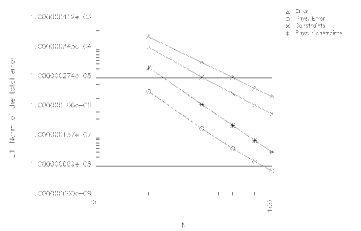
Figure 1: Total error with respect to the exact solution for the standard compactification, for $N$=20,40,60,80 and 100 points in the $x$-direction

In Fig. 1 we plot the error summed over all fields and the constraint violation for the whole grid and for the physical part, $\Omega\geq 0$, at coordinate time $t=2.1$ for increasing number of grid points $N$, the initial time is $t_{ini}=1.8$. This yields a convergence order for the total error of $2.903\pm 0.002$, which is in good agreement with our expectation of a third order scheme. The total constraint violation converges to zero with order $3.32\pm 0.08$. The physical errors are both much smaller than the total error, which comes from the fact, that the error is concentrated at the boundary, which does not lie in the physical space-time.

A problem we face at the moment is, that the behaviour of the error does not generalize to higher grid dimensions. There fast growing instabilities arise at the boundary, which are not present at lower resolutions. These instabilities dominate the total error after a short time and lead to a crash at the boundary.

Numerical Properties of I

The great advantage of the conformal approach, that the boundary of the grid does not lie in the physical space-time, in opposite to the other approaches in numerical relativity, can be further illustrated with the following example. We start with initial data from the standard compactification and add during the evolution uniform random noise to the exact values for the ingoing characteristic fields at the boundary. The maximum of the noise is $\delta=0.005$, we use $40\times 79$ grid points, initial time is $t_{ini}=1.8$. We plot in Fig. 2 the quantity $C=|E_{ab}E^{ab}+B_{ab}B^{ab}|$ composed out of the electric and magnetic part of the Weyl tensor. In an undisturbed evolution $C$ remains zero all the time, because $E_{ab}=B_{ab}=0$ in the initial data and this is preserved through the numerical evolution.

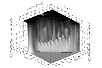
Figure 2: $C=|E_{ab}E^{ab}+B_{ab}B^{ab}|$ for the standard compactification with noise entering through the boundary. The black line indicates I ($\Omega=0$).

In Fig. 2 one can see two crucial points. First I is not affected at all by the noise from the boundary. This means, that I is stable under small perturbations entering from the unphysical part. Second the noise from the boundary, which is also added to the Weyl tensor, enters the grid, but does not enter the physical space-time. Note that the scale of the plot is $10^{-7}$ and the plot is cut off at $1.2\times 10^{-7}$. The plot would have been $1000$ times bigger to cover the whole range of $C$. So I is indeed a characteristic hypersurface not only analytically but also with great accuracy numerically. Near $i^{+}$ at $t=\pi$ a small amount of noise enters the physical space-time, but this seems to be related to the very poor resolution of the physical space-time in this area.

Further support for the property of I can be gained by the following Fig. 3 of the error and constraint violation for the whole grid and the physical part.

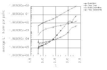
Figure 3: Error and constraint violation for the standard compactification with noise entering through the boundary.

It can clearly be seen, that the physical error is much smaller than the total error, the same is valid, but not with the same accuracy, for the constraint violation. The reason for this might be, that one calculates the physical constraint violation at points, where $\Omega\geq 0$, but through the discretization for the derivatives one gets an influence from points outside of the physical space-time. Both the physical error and the constraint violation in the physical part grow rapidly, while approaching $i^{+}$ at $t=\pi$, which has the reason in the low number of physical grid points shortly before $i^{+}$. This behavior of the error and the constraint violation is not limited to this special case. Also for all other tested space-times, one can see, that the error in the physical part is small relative to the error in the unphysical part. We have made several movies, where one can see, that the error stays outside of I. These movies are available on our home page Hom .

Reproducing the static Einstein universe

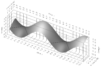
Figure 4: The conformal factor $\Omega$ for the standard compactification at $z=0$. The black line indicates I ($\Omega=0$)

In Fig. 4 we plot the conformal factor of the standard compactification, where we give the exact values for the ingoing characteristic fields during the evolution. It can be seen, that the physical space-time bounded by I shrinks to a point $i^{+}$, so it is no problem to reach $i^{+}$ and continue in a smooth way. In principle it is now physically meaningless to continue the evolution, because the whole physical part has been calculated. But from the numerical point of view it is interesting to see, for how long it is possible to evolve further, before the code crashes. The plot shows, that it is possible to calculate additional one and a half copies of Minkowski space-time. As the Minkowski space-time is embedded in the static Einstein universe, we obtain nothing else but a part of the static Einstein universe.

Conformal Gauges

As we have pointed out in II in the conformal picture there is one additional gauge freedom apart from the coordinate gauge and the tetrad gauge. We are allowed to rescale the conformal factor and the metric according to $\Omega\rightarrow\omega\Omega,g_{ab}\rightarrow\omega^{2}g_{ab}$, where $\omega$ has to be strictly positive, so that the asymptotic structure is conserved by this conformal rescaling.

For the second conformal manifold (IV.2.1) we tested different conformal gauges. Some of these gauges lead to a very fast exponential growth of the error and were therefore useless. The most successful choice was the gauge:

$$\omega=\frac{1}{1+x^{2}+z^{2}},$$

which made many components spatially constant. It is therefore not too surprising, that this solution had the smallest exponential growth of the error. Motivated by this gauge, we tried another time dependent one, which should model a nearly constant factor $\omega$ in the physical space-time and then a decaying factor in the unphysical space-time in order to have very small values at the boundary:

$$\omega=\frac{1}{1+(x^{2}+z^{2})t}$$

This function has the serious drawback, that it forms a sharp peek at the axis as time increases. This results in also very peeked solutions, which leads to a more rapid exponential growth of the error.

These results are illustrated in the next plot (Fig. 5).

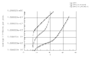
Figure 5: The effect of different conformal gauges on the total error for the second compactification of Minkowski (IV.2.1) space-time, grid: $40\times 79$, $t_{ini}=1.3$

As the exponential growth is different for the chosen gauges, it seems, as if different exponentially growing solutions are excited. We do not know, whether this difference emerges already on the level of the conformal field equations or on the level of the numerical implementation. As the exponential growth is a serious problem for long term runs, this has to be further examined in the future.

Comparison of the three compactifications

Before we conclude the section on the Minkowski space-time, we would like to illustrate the long term behavior of the three different compactifications in Fig. 6.

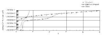
Figure 6: The long term behavior of the total error of three different compactifications of Minkowski space-time, the marks are set every 1000 time steps, grid size: $40\times 79$

The absolute value is not comparable, because the step size is not the same for the three cases. But the exponential growth can be compared, because in principle this should not depend on the step size. As expected, the fully static solution runs for the longest time. The big difference in the stability between the standard compactification and the light-like compact one seems to arise, because of the greater spatial variance of the light-like compact solution.

IV.2.2 Boost-axisymmetric solution of Bičák and Schmidt

As a further testbed for our code, we chose an asymptotically flat solution from the general class of boost-axisymmetric space-times analysed by Bičák and Schmidt Bičák and Schmidt (1989). Since we are working in the conformal picture it is necessary, that the solution admits a regular $\mbox{ I}^{+}$ and is regular on the axis. Indeed there is a whole family of such solutions in the class of boost-axisymmetric solutions, which fulfills these conditions, except for two singular points on $\mbox{ I}^{+}$, see Bičák et al. (1983). This family of solutions describes two self-accelerating particles and the singular points on $\mbox{ I}^{+}$ are the places, where the particles hit $\mbox{ I}^{+}$.

$$ds^{2} = e^{\lambda}\left(\frac{(xdx+ydy)^{2}}{x^{2}+y^{2}}-\frac{(tdt-zdz)^{2}}{t^{2}-z^{2}}\right)$$

$$+e^{-\mu}\frac{(xdy-ydx)^{2}}{x^{2}+y^{2}}+e^{\mu}\frac{(tdz-zdt)^{2}}{t^{2}-z^{2}}$$

$$\Omega = -t^{2}+x^{2}+y^{2}+z^{2}$$

with

$$\mu(x^{2}+y^{2},t^{2}-z^{2}) = m(t^{2}-z^{2}-x^{2}-y^{2}),$$

$$\lambda(x^{2}+y^{2},t^{2}-z^{2}) = m^{2}(x^{2}+y^{2})^{2}-m(x^{2}+y^{2}+t^{2}-z^{2}),$$

where $m$ is a free parameter. In the limit $m\rightarrow 0$ the solution approaches Minkowski space-time. In order to avoid the singularities in the evolution we chose our hyperboloidal initial data hypersurface in the future of the singular points and so we are able to calculate the rest of the space-time up to $i^{+}$.

We first show an error plot in Fig. 7 for a run with $m=1.75$ and a grid of $40\times 79$ points, which shows, that there is no problem to reach $i^{+}$ at $t=0$ and to evolve further.

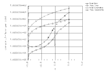
Figure 7: Error and constraint violation for the boost-axisymmetric solution with strong data $m=1.75$, grid size: $40\times 79$

The high difference between total and physical error arises, because of the very high values near the grid boundary. This error does only enter the physical space-time to a certain degree, which shows again the advantage of the conformal approach to have the boundary in the unphysical part of the space-time together with a characteristic hypersurface I, which separates the unphysical from the physical part.

To show that this case is non-trivial in the sense that the curvature does not vanish we plot in Fig. 8 the quantity $C=|E_{ab}E^{ab}+B_{ab}B^{ab}|$.

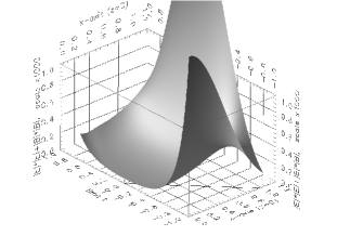
Figure 8: $C=|E_{ab}E^{ab}+B_{ab}B^{ab}|$ for the boost-axisymmetric solution with $m=1.75$. Note the scale of 1000. The black line indicates I

The scale of the plot indicates, that we are really dealing with data in the non-linear regime and that the numerical scheme can deal with large gradients in the data.

V Summary

In this article we have presented a new code for simulating axisymmetric, isolated systems in general relativity. We have implemented the axisymmetry by adapting the cartoon method to the tetrad formalism and formulated boundary conditions, which are compatible with the symmetric hyperbolic principal part of our evolution equations. We have tested the numerical scheme by applying it to the axisymmetric scalar wave equation. The results show, that we can solve the wave equation in a stable and convergent way, by choosing a suitable interpolation scheme for the cartoon method. The fact that the code is still unstable for the quasilinear conformal field equations needs to be examined in further detail.

The numerical test for the conformal field equations with hyperboloidal initial data from different compactifications of the Minkowski space-time and strong data from a family of boost-axisymmetric space-times show, that the semi-global simulation of space-times until $i^{+}$ and further on is possible. In addition, we have demonstrated, that I is also numerically a characteristic hypersurface and acts as a boundary between physical and unphysical space-time with good accuracy.

There remain several tasks. We need to develop modules to extract the radiation on I and to determine the Bondi mass. These are straightforward implementations of the algebraic transformation between our tetrad and the tetrad adapted to I. Furthermore, we need to improve our boundary conditions to be at least third order accurate so that we do not loose one order of global accuracy as we do now. An analysis of the initial boundary value problem needs to be carried out (possibly along the lines of Friedrich and Nagy (1998)) in order to be able to provide boundary conditions which are compatible with the constraints. This would minimize the influence of constraint violating modes generated at the boundary.