On discretizations of axisymmetric systems

Abstract

In this paper we discuss stability properties of various discretizations for axisymmetric systems including the so called cartoon method which was proposed by Alcubierre, Brandt et.al. for the simulation of such systems on Cartesian grids. We show that within the context of the method of lines such discretizations tend to be unstable unless one takes care in the way individual singular terms are treated. Examples are given for the linear axisymmetric wave equation in flat space.

I Introduction

Axisymmetric systems are notorious for the difficulties they pose in numerical simulations when they are expressed in coordinates adapted to the symmetry. The problem is due to the singular nature of the coordinates on the axis, i.e., the set of fixed points for the symmetry transformations or, equivalently, the set where the infinitesimal generator of the symmetry – the Killing vector – vanishes. Adapted coordinates, i.e., an angle $\phi$ along the Killing vector, a radius $r$ measuring ‘distance’ from the axis and a third coordinate $z$, yield coordinates $(r,z)$ on the space of orbits of the action of the symmetry group. The general theory of group actions Jänich (1968); Frauendiener (1987) yields the following facts. The orbit space contains two types of orbits: the ‘regular orbit’ is a circle around the axis. It has maximal dimension (one) and the union of all regular orbits is dense in the space of orbits. The other type of orbit is a fixed point which has dimension zero. The set of fixed points is a submanifold of codimension two, the ‘axis’. The drop in dimension of the orbits shows up in the topology of the space of orbits which acquires a boundary corresponding to the axis points and in a degeneracy of the adapted coordinates: since on the axis (for fixed $z$) all values of $\phi$ address the same point the angular coordinate becomes irrelevant on the axis, so that the coordinate system degenerates there.

Invariant tensor fields transform in a rigid way (Lie transport) under the symmetry so that they are determined on an entire regular orbit once they are known on one of its points. Therefore, in order to determine the fields on the entire space it is enough to determine them on a hypersurface which is transversal to the orbits. Thus, the problem is reduced to a problem in a space with lower dimension. For invariant tensor fields at a fixed point the invariance implies a transformation law among the tensor components which must be interpreted as a regularity condition for the tensor field on the axis.

The advantage of using the adapted coordinates is, of course, the manifestation of this reduction. In these coordinates the components of the tensor fields do not depend on the angular coordinate along the Killing vector. Thus, there are only two essential coordinates left over and the problem reduces in complexity because an axisymmetric problem on some open 3-dimensional domain reduces to an equivalent 2D-problem on a domain with boundary. The boundary conditions are obtained from regularity conditions on the axis.

The disadvantage of using the adapted coordinates is that the reduced equations become formally singular on the axis. The regularity conditions on the axis guarantee that the individual terms in the equation have in fact a regular limit on the axis so there is not a real problem. Yet, numerically, one has to evaluate terms which are formally $0/0$ or $\infty-\infty$ which does pose problems. Thus, it seems that one has the choice between a 3D system with regular, such as Cartesian, coordinates and regular equations or a 2D system with degenerate coordinates and singular equations.

In an attempt to combine the best of both worlds, Alcubierre et al. Alcubierre et al. (1999) proposed what they called the cartoon method. This scheme was designed to borrow from the singularity-free nature of full 3D Cartesian coordinates $x$, $y$, $z$ and to allow the treatment of axisymmetric problems without the memory constraints of a full 3D problem. The method uses the Killing transport equation along the orbits to find the field values on the grid points of a Cartesian grid from its values on the hypersurface $y=0$. These values are obtained by interpolation from the grid points lying in that hypersurface. For a second order method one needs to keep only three hypersurfaces $y=const$ in memory so that the problem scales quadratically with the number of points and not cubically.

The plan of the paper is as follows. In section II we discuss the cartoon method in more detail. In order to have a specific problem at hand we apply it to the axisymmetric linear wave equation in section III. We write this equation as a first order symmetric hyperbolic system. The reason for this apparent complication is that we have implemented this method for the axisymmetric conformal field equations which are a symmetric hyperbolic system and because the linear wave equation served as a model equation to test various implementations Frauendiener and Hein (2002). It turns out that the crucial ingredient to the method is the interpolation and we discuss various possibilities. Furthermore, we show that there is no real difference between the cartoon method using Cartesian coordinates and the formulation in adapted coordinates so that the issues which are relevant for the former apply to the latter as well. In section IV we analyse the stability properties of the cartoon method with different interpolation procedures as well as other possible discretizations when the method of lines is used for time evolution. We end with a brief discussion of the results.

II The Cartoon method

In this section we present the cartoon method in more detail. We consider a 3-dimensional Euclidean space ${\mathcal{E}}^{3}$ with Cartesian coordinates $\mathbf{x}=(x,y,z)$ on which we define the action of the circle group $SO(2)=G$

$$G=\left\{g=\left(\begin{smallmatrix}a&-b\\ b&a\end{smallmatrix}\right)\mid a^{2}+b^{2}=1\right\}$$

in the usual way by

$$\begin{split}\Phi:\left(G,{\mathcal{E}}^{3}\right)&\to{\mathcal{E}}^{3},\\ \left(g,\mathbf{x}\right)&\mapsto\Phi(g,\mathbf{x})=(ax-by,bx+ay,z)=g\cdot\mathbf{x}.\end{split}$$ (1)

The infinitesimal generator of this action is the vector field $\xi=x\partial_{y}-y\partial_{x}$ which vanishes on the axis $x=y=0$, the set of fixed points for the action. The action $\Phi$ is the prototype for any axisymmetric system in the neighbourhood of the axis in the sense that for any of these systems one can find local coordinates in which the action takes the above form Jänich (1968); Frauendiener (1987). Therefore, we will focus here on flat space because we are mainly interested in the local properties in a neighbourhood of the axis. Curvature will not play an essential role.

Introducing adapted cylindrical coordinates $(r,\phi,z)$ the coordinate expression for the action is

$$\left(\left(\begin{smallmatrix}\cos\theta&-\sin\theta\\ \sin\theta&\cos\theta\end{smallmatrix}\right),(r,\phi,z)\right)\mapsto(r,\phi+\theta,z)$$

and the Killing vector is given by

$$\xi=\partial_{\phi}.$$

These coordinates are singular on the axis which can be seen e.g., from the fact that the Jacobi matrix of the transformation between cylindrical and Cartesian coordinates has vanishing determinant there.

A tensor field $T$ in ${\mathcal{E}}^{3}$ is axisymmetric if for any $g\in G$ it satisfies the condition

$$\Phi_{g}^{*}T=T$$ (2)

where $\Phi_{g}^{*}$ denotes the pull-back with $\Phi_{g}:{\mathcal{E}}^{3}\to{\mathcal{E}}^{3},\mathbf{x}\mapsto g\cdot\mathbf{x}$. This condition expresses the invariance of $T$ with respect to the action of $SO(2)$. The infinitesimal version of this condition is the equation of Killing transport

$${\mathcal{L}}_{\xi}T=0.$$ (3)

Suppose we want to solve a quasi-linear system of PDEs of the form

$$\dot{T}=F(\partial_{a}T,T,t,\mathbf{x})$$ (4)

where $T$ is some given time dependent axisymmetric tensor field on ${\mathcal{E}}^{3}$. Here, $\partial_{a}$ denotes covariant differentiation. The usual way to treat this system is to express it in terms of the adapted coordinates and to use the invariance condition (3) which asserts, that the components of $T$ in the basis of adapted coordinates do not depend on $\phi$. Thus, the essential coordinates are $r$ and $z$ and the problem is reduced to a 2-dimensional one. However, from the form of the covariant derivative operator, i.e., the Christoffel symbols of the metric expressed in cylindrical coordinates it is clear, that the equation will, in general, contain singular terms.

A different procedure is to employ any coordinate system which is regular in a neighbourhood of the axis and then to make explicit use of the invariance condition (2) or its infinitesimal version (3) Thornburgh (2002). So we may choose Cartesian coordinates with the axis at $x=y=0$. Let $T$ be an arbitrary axisymmetric tensor field on ${\mathcal{E}}^{3}$. From the invariance condition (2) we can find its values at any point in ${\mathcal{E}}^{3}$ from its values on the half-plane ${\mathcal{H}}=\{y=0,x\geq 0\}$. To illustrate this let us first assume that $T$ is a scalar field. From the invariance condition we have

$$T(\mathbf{x})=T(g\cdot\mathbf{x})$$

for any rotation matrix $g$ and each point $\mathbf{x}=(x,y,z)$. Thus, in particular, choosing

$$g=\begin{pmatrix}\frac{x}{\sqrt{x^{2}+y^{2}}}&\frac{y}{\sqrt{x^{2}+y^{2}}}\\ \frac{-y}{\sqrt{x^{2}+y^{2}}}&\frac{x}{\sqrt{x^{2}+y^{2}}}\end{pmatrix}$$

for $x\neq 0$, $y\neq 0$ we have $\Phi_{g}(\mathbf{x})=(r,0,z)$ with $r=\sqrt{x^{2}+y^{2}}$ so that

$$T(\mathbf{x})=T(r,0,z).$$ (5)

Similarly, if $T=T_{1}\,dx+T_{2}\,dy+T_{3}\,dz$ is a 1-form, we have

$$\Phi_{g}^{*}T(\mathbf{x})=T_{1}(g\cdot\mathbf{x})\,d(\Phi_{g}^{*}x)+T_{2}(g\cdot\mathbf{x})\,d(\Phi_{g}^{*}y)+T_{3}(g\cdot\mathbf{x})\,d(\Phi_{g}^{*}z).$$

Inserting the explicit form of the matrix $g$ yields

$$\Phi_{g}^{*}T(\mathbf{x})=T_{1}(g\cdot\mathbf{x})\,\left(a\,dx-b\,dy\right)+T_{2}(g\cdot\mathbf{x})\,\left(b\,dx+a\,dy\right)+T_{3}(g\cdot\mathbf{x})\,dz\\ =\bigl{(}aT_{1}(g\cdot\mathbf{x})+bT_{2}(g\cdot\mathbf{x})\bigr{)}\,dx+\bigl{(}aT_{2}(g\cdot\mathbf{x})-bT_{1}(g\cdot\mathbf{x})\bigr{)}\,dy+T_{3}(g\cdot\mathbf{x})\,dz$$

so that, in this case, the invariance condition implies the three equations

$$T_{1}(\mathbf{x})=aT_{1}(g\cdot\mathbf{x})+bT_{2}(g\cdot\mathbf{x}),$$

$$T_{2}(\mathbf{x})=-bT_{1}(g\cdot\mathbf{x})+aT_{2}(g\cdot\mathbf{x}),$$

$$T_{3}(\mathbf{x})=T_{3}(g\cdot\mathbf{x}).$$

Choosing, as before, $a=x/\sqrt{x^{2}+y^{2}}$ and $b=-y/\sqrt{x^{2}+y^{2}}$, we get the relations

$$T_{1}(\mathbf{x})=\frac{1}{r}\,\left(x\,T_{1}(r,0,z)-y\,T_{2}(r,0,z)\right),$$

$$T_{2}(\mathbf{x})=\frac{1}{r}\,\left(y\,T_{1}(r,0,z)+x\,T_{2}(r,0,z)\right),$$ (6)

$$T_{3}(\mathbf{x})=T_{3}(r,0,z).$$

Similar relations hold for tensor fields with different type. This shows that we can get information about the values at all points outside the axis from values at the points on ${\mathcal{H}}$ except for the axis. On the axis these relations imply regularity conditions for the tensor fields. E.g., in the case of a 1-form above we get $T_{1}(0,0,z)=T_{2}(0,0,z)=0$ which follows by taking limits from various directions towards the axis points.

How are we to use this analytical background in numerical applications? Following Alcubierre et al. (1999) we cover the half-plane ${\mathcal{H}}$ by a regular Cartesian grid

$$x_{i}=i\Delta x,z_{k}=k\Delta z,\text{ with }i,k\in{\mathbb{Z}},i\geq 0$$

which we think of as being a part of a full 3D cartesian grid with points given by $x_{i},y_{j},z_{k}$ with $y_{0}=0$. Each component of a tensor field $T$ yields a grid function $T_{ijk}$. The axisymmetry implies that we should be able to determine the functions $T_{ijk}$ from their values on ${\mathcal{H}}$ alone.

In order to treat equations like (4) above one needs to compute approximations to the spatial derivatives of the components. This is straightforward in the case of $x$- and $z$-derivatives. However, for the $y$-derivatives we need to find the values of the grid functions at points outside ${\mathcal{H}}$.

Figure 1: Illustration of the method (see text)

The situation is illustrated in Fig. 1. It shows the view from the positive $z$-axis down onto the $(x,y)$-plane. The black dots indicate grid points in ${\mathcal{H}}$, the point on the left with the cross being the axis. The open circles indicate points outside ${\mathcal{H}}$ with $y=\pm\Delta y$. The values of the fields at these points have to be computed from the invariance equation (2). Following the orbits through these outside points one can connect them with points in ${\mathcal{H}}$, indicated by the open squares, and one can find the values at the outside points from the values at these points on ${\mathcal{H}}$. Thus, e.g., applying (5) in this situation we obtain for a scalar

$$T(x_{i},\pm\Delta y,z_{k})=T(\sqrt{x_{i}^{2}+\Delta y^{2}},0,z_{k}),$$

while the corresponding transformation for a 1-form follows from (6). Note, that the squares are on ${\mathcal{H}}$ but they are not, in general, grid points. Thus, having reduced the problem to ${\mathcal{H}}$ the remaining question is how to determine the values at these points. The natural choice is to use some form of interpolation as it is also suggested in Alcubierre et al. (1999). However, it is not clear what kind of interpolation should be used and it is the purpose of this work to point out that not all interpolation schemes perform well.

III The axisymmetric wave equation

To have a concrete example at hand we will focus now on the axisymmetric scalar wave equation in flat space. It is clear from the considerations above that the $z$-dependence is irrelevant for this analysis. Therefore, we simplify even further by assuming that the field is in fact axisymmetric and $z$-independent. Then the equation is

$$\ddot{\phi}=\phi_{xx}+\phi_{yy}$$

where $\phi=\phi(t,x,y)$ is axisymmetric. Introducing the 1-form $d\phi=u\,dt+v\,dx+w\,dy$ we can derive from this equation a symmetric hyperbolic first order system

$$\dot{u}=v_{x}+w_{y},$$ (7)

$$\dot{v}=u_{x},$$ (8)

$$\dot{w}=u_{y}$$ (9)

with the constraint $v_{y}-w_{x}=0$. The function $\phi$ can be recovered from a solution of this system by either evolving $\dot{\phi}=u$ or by solving $\Delta\phi=v_{x}+w_{y}$ at each time step. Since $\phi(t,x,y)=\phi(t,\sqrt{x^{2}+y^{2}},0)=\phi(t,\pm x,\pm y)$ we have, in particular, $w(t,x,0)=0$ and $v(t,0,0)=0$. Furthermore, taking derivatives we obtain $u_{y}(t,x,0)=0$ and $v_{y}(t,x,0)=0$. Hence, we can forget about (9) and the constraint, because these equations are identically satisfied on ${\mathcal{H}}$. So we are left with the system

$$\dot{u}=v_{x}+w_{y},$$ (10)

$$\dot{v}=u_{x}.$$ (11)

Before we go into the more numerical details it is worthwhile to write down the system in adapted (i.e., cylindrical) coordinates $(r,\phi,z)$

$$\dot{u}=v_{r}+\frac{v}{r},\qquad\dot{v}=u_{r},$$ (12)

which follows by expressing the Laplace operator in these coordinates, using the independence of $z$ and $\phi$ and then introducing the first derivatives as new dependent variables.

We solve these equations numerically by applying the method of lines, i.e., we discretize the spatial derivatives to obtain a system of ODEs. This can then be solved with standard ODE solvers. We put the equations on a grid as indicated above. Now ${\mathcal{H}}$ is in effect a 1-dimensional grid with points $x_{i}=i\Delta x$ and we have grid functions $u_{i}(t)=u(t,i\Delta x,0)$, $v_{i}(t)=v(t,i\Delta x,0)$. According to the idea of the cartoon method we compute the term $w_{y}$, which of course does not vanish on ${\mathcal{H}}$, by following the orbits. From the transformation law (6) for a 1-form we get

$$w(t,x,y)=\frac{y}{\sqrt{x^{2}+y^{2}}}\;v(t,\sqrt{x^{2}+y^{2}},0).$$ (13)

The discretization of the term $w_{y}$ using centered differences to get a second order accurate approximation yields

$$w_{y}(t,x_{i},0)=\frac{w(t,x_{i},\Delta y)-w(t,x_{i},-\Delta y)}{2\Delta y}=\frac{v_{*}}{x_{*}},$$

where $x_{*}=\sqrt{x_{i}^{2}+\Delta y^{2}}$ and $v_{*}=v(t,x_{*},0)$. This, then, yields the final system obtained by application of the cartoon method

$$\dot{u}=v_{x}+\frac{v_{*}}{x_{*}},\qquad\dot{v}=u_{x}.$$ (14)

It is instructive to compare this system with the system (12) obtained in adapted coordinates. Expanding in powers of $\Delta y$ we get

$$\frac{v_{*}}{x_{*}}=\frac{v(x_{*})}{\sqrt{x_{i}^{2}+\Delta y^{2}}}=\frac{v_{i}}{x_{i}}+\frac{1}{2}\left(\frac{\partial v}{\partial x}(x_{i})-\frac{v_{i}}{x_{i}}\right)\frac{\Delta y^{2}}{x_{i}^{2}}+{\mathcal{O}}(\Delta y^{4}).$$

Hence, up to the accuracy $\Delta y^{2}$ for which the derivation of (14) is valid, the two systems agree.

One can, in fact, say even more. The infinitesimal invariance condition (3) or, equivalently, taking the $y$-derivative of (13) and evaluating at $y=0$ yields

$$w_{y}(t,x,0)=\frac{v(t,x,0)}{x}$$

for all $x>0$. Hence, whenever we use the cartoon method to approximate $w_{y}$ to a certain order in the grid spacing $\Delta y$ we approximate $v/x$ to the same order. Thus, there is no difference in that order of accuracy between the systems (14) and (12). And, therefore, the discussions in the following section apply to both.

IV Numerical issues

In this section we discuss the stability properties of various implementations of the systems (12) and (14). In the spirit of what was said in the previous section we regard the term $\frac{v_{*}}{x_{*}}$ as an approximation to $\frac{v}{x}$ which is not necessarily located on a grid point. Then, the main question is how to approximate this term on ${\mathcal{H}}$. We implement several possibilities and look at their stability properties.

In order to have a well defined problem we have to worry about boundary conditions at the origin $x=0$ and at an outer boundary which we put at $x=1$. The conditions at the origin follow from the transformation properties of the fields under the symmetry. They are

$$v(t,-x,0)=-v(t,x,0)\rightarrow v(t,0,0)=0,$$ (15)

$$u(t,-x,0)=u(t,x,0)\rightarrow\frac{\partial u}{\partial x}(t,0,0)=0.$$ (16)

The fact, that $x=0$ is the fixed point of the symmetry is reflected in the simultaneous vanishing of $v$ and $x$. This also implies that at the origin we have $\frac{v}{x}=v_{x}$ so that at $x=0$ the time evolution of $u_{0}=u(t,0,0)$ is given by the equation $\dot{u}_{0}=2v_{x}(t,0,0)$.

Since we are interested in the properties of the scheme in the interior we implement some sort of periodic boundary conditions. Since we want to avoid a second origin at $x=1$ we imagine that our wave equation lives on a 2-sphere and is symmetric under rotations of the sphere around its poles. Now we impose the condition that it be also symmetric under reflection across the equator. This discrete symmetry allows us to consider the equation only along a meridian from the north pole down to the equator. The symmetry implies conditions for the fields at the equator which we put at $x=1$:

$$v(t,1-x,0)=-v(t,1+x,0)\rightarrow v(t,1,0)=0,$$ (17)

$$u(t,1-x,0)=u(t,1+x,0)\rightarrow\frac{\partial u}{\partial x}(t,1,0)=0.$$ (18)

In the context of the method of lines we write down a system of ODEs for the grid functions $v_{i}$ and $u_{i}$. This will be a linear system of the form $\dot{f}=\mathbf{A}f$ and we can find its stability properties by looking at the spectrum of the matrix $\mathbf{A}$ which we determine numerically.

With these preparations out of the way we can now write down the first of our discretizations for the system (12). This is the first one which comes to mind, namely

$$\begin{aligned} \dot{u}_{0}&=\frac{2v_{1}}{h},\\ \dot{u}_{i}&=\frac{v_{i+1}-v_{i-1}}{2h}+\frac{v_{i}}{ih},\\ \dot{u}_{N}&=-\frac{v_{N-1}}{h}\\ \end{aligned}\qquad\begin{aligned} \dot{v}_{0}&=0,\\ \dot{v}_{i}&=\frac{u_{i+1}-u_{i-1}}{2h}\\ \dot{v}_{N}&=0.\end{aligned}$$ (19)

Here we have chosen $h=1/N$ where $N+1$ is the number of grid points so that $x_{i}=ih$. The matrix $\mathbf{A}$ which corresponds to this discretization has dimensions $2(N+1)\times 2(N+1)$ and the form

$$\mathbf{A}=\frac{1}{h}\left(\begin{array}[]{c|c}0&\mathbf{C}\\ \hline\cr\mathbf{D}&0\end{array}\right)$$

where $\mathbf{C}$ is the matrix

$$\mathbf{C}=\left(\begin{array}[]{cccccc}0&2&0&\cdots&&\\ -\frac{1}{2}&1&\frac{1}{2}&&&\\ &-\frac{1}{2}&\frac{1}{2}&\frac{1}{2}&&\\ &&\ddots&\ddots&\ddots&\\ &&&-\frac{1}{2}&\frac{1}{N-1}&\frac{1}{2}\\ &&\cdots&0&-1&0\end{array}\right)$$

and $\mathbf{D}$ is

$$\mathbf{D}=\left(\begin{array}[]{ccccc}0&0&\cdots&0&0\\ -\frac{1}{2}&0&\frac{1}{2}&&\\ &\ddots&\ddots&\ddots&\\ &&-\frac{1}{2}&0&\frac{1}{2}\\ 0&0&\cdots&0&0\\ \end{array}\right).$$

This system of ODEs is solved by a standard ODE solver, such as a Runge-Kutta scheme or a multistep scheme like the Adams-Bashforth schemes. We also consider the ‘iterated Crank-Nicholson’ (ICN) scheme which has become popular among numerical relativists (see Teukolsky (2000) for an analysis of this scheme). Relevant for deciding about the stability of a difference approximation for ODEs is the region of absolute stability (see e.g. Hairer et al. (2000); Hairer and Wanner (1996)). This is a closed set $\Omega$ in the complex plane which consists of those $z=\lambda\Delta t\in{\mathbb{C}}$ for which the method applied to the equation $\dot{u}=\lambda u$ with step size $\Delta t$ produces bounded approximations. The stability regions for the schemes mentioned above are shown in appendix A and the stability region(s) for ICN is determined in appendix B.

Thus, in the context of the method of lines, the stability conditions can be obtained by determining the eigenvalues of the discretization matrix $\mathbf{A}$ and checking whether it is possible to scale it so that it fits entirely into the stability region of the ODE solver. The scale factor determines the maximal admissible time step. Strictly speaking, this consideration applies only to the linear case. For non-linear equations this check should be understood as a ‘rule of thumb’ Trefethen (2000).

The spectrum $\sigma_{N}(h\mathbf{A})$ of $h\mathbf{A}$ is shown for $N=100$ in Fig. 2.

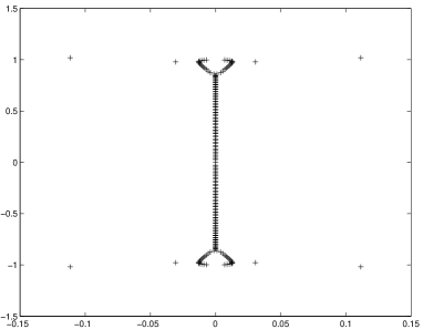
Figure 2: Spectrum of the ‘straightforward’ discretisation, scheme 2a

We point out some of its properties which are valid for all other discretizations below as well. The spectrum is symmetric with respect to reflections about the real axis as well as about the imaginary axis. While the former symmetry is due to the reality of the equation, the latter is a consequence of the fact that the underlying equation is a second order wave equation which has in- and outgoing modes. Furthermore, the spectrum is concentrated mostly on the imaginary axis with a few ‘outliers’. It can be seen that the eigenvalues with the largest, in absolute value, real part remain unchanged when we change $N$ which implies that the spectral radius of $\mathbf{A}$ is proportional to $N$.

An interesting feature of the spectrum are the two ‘handles’ which are located near $\pm\mathrm{i}$. These, and the outliers are due to the $v/x$ term in the equation and, depending on the particular discretization scheme, they may or may not be present as we will see below. Since the eigenvalues of the corresponding continuous system are given by $\pm\mathrm{i}\lambda_{k}$, where $\lambda_{k}$ is the k-th zero of the Bessel function $j_{1}$, all the eigenvalues with nonvanishing real part are spurious, i.e., they do not have an analogue in the continuous problem. Thus, the corresponding eigenvectors are parasitic modes because they do not approximate a regular mode.

When combined with a time integrator this spectrum and the stability region of the integrator decide about the stability of the overall scheme. The stability regions of some ODE solvers are sketched in appendices A and B. Some of these include an interval on the imaginary axis while others include only the origin. All the stability regions extend further into the left half plane than into the right. This implies that if a spectrum contains points in the right plane (i.e., modes with positive real part) then these modes tend to either unnecessarily diminish the time step because they have to be scaled into the stability region (if the stability region of ODE solver extends into the right half plane int he first place) or else they create instabilities.

Another possibility to overcome instabilities is the addition of numerical dissipation. This has the effect that the spectrum of $\mathbf{A}$ is shifted towards the left. However, the presence of the handles and of the outliers implies that the amount of dissipation necessary for stabilising the scheme is rather high compared to cases where the spectrum is located entirely on the imaginary axis. This means that the evolution cannot be followed accurately because ultimately the waves will be damped out. Thus, the appearance of handles and outliers seems to leave us with the choice between the Scylla of instability and Charybdis of inaccuracy. Therefore, we take the appearance of these modes as a sign for an inadequate scheme.

The discretizations which we have looked at can be divided into three groups. Discretizations of the system (14) obtained from the cartoon method of computing the transversal derivatives, 2nd order discretizations of the system (12) and three somewhat non-standard discretizations of that system. In the list given below we only show the formula for the inner points of the grid. The values at the boundary points are obtained by using the appropriate symmetry conditions. Furthermore, we omit the equation for $\dot{v}_{i}$ in those cases where its discretization is the same as for the derivative term in the $\dot{u}_{i}$ equation.

1. Using the cartoon approximation we discretize the system (14) to second order in $h$. The derivatives are taken to be centered in all the three different schemes, while we use different interpolations for the term $\frac{v_{*}}{x_{*}}$.

   1. Two point interpolation (see Fig. 3):

      $$\dot{u}_{i}=\frac{v_{i+1}-v_{i-1}}{2h}+\frac{(x_{i+1}-x_{*})v_{i}+(x_{*}-x_{i})v_{i+1}}{hx_{*}}.$$

   2. Three point interpolation (see Fig. 3):

      $$\dot{u}_{i}=\frac{v_{i+1}-v_{i-1}}{2h}+\sum_{j=-1}^{1}p_{i+j}(x_{*})v_{i+j},$$

      where $p_{i-1}(x)=(x-x_{i})(x-x_{i+1})/2h^{2}$, $p_{i}(x)=-(x-x_{i+1})(x-x_{i-1})/h^{2}$ and $p_{i+1}(x)=(x-x_{i})(x-x_{i-1})/2h^{2}$.

      

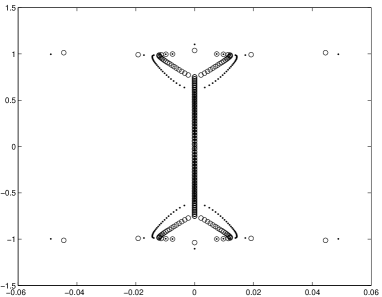
      Figure 3: Two (dots) and three (circles) point interpolation of the cartoon method, schemes $1a$, $1b$

   3. Centered two point interpolation (see Fig. 4):

      $$\dot{u}_{i}=\frac{v_{i+1}-v_{i-1}}{2h}+\frac{(x_{i+1}-x_{*})v_{i-1}+(x_{*}-x_{i-1})v_{i+1}}{2hx_{*}}.$$

      

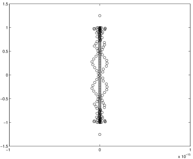
      Figure 4: Centered two point interpolation for the cartoon method, scheme $1c$

   It is obvious that the interpolation in schemes $1a$ and $1b$ is not useful because of the appearance of the handles and the outliers. This suggests that for higher order Lagrange interpolation one has to expect the same kind of behaviour. In fact, in our studies related to Frauendiener and Hein (2002) we find that e.g. 5th order Lagrange interpolation is as unstable as interpolation using Chebyshev polynomials. However, the fact that scheme $1c$ yields a purely imaginary spectrum (up to round-off error) suggests that the use of the centered interpolation is advantageous. In view of the fact that the cartoon method provides an approximation of the $1/x$ term in (12) we now look at this system directly.

2. Three second order discretizations of the system (12).

   1. The scheme discussed already above (see Fig. 2)

      $$\dot{u}_{i}=\frac{v_{i+1}-v_{i-1}}{2h}+\frac{v_{i}}{ih}.$$

   2. A centered approximation for the numerator of the second term (see Fig. 5)

      $$\dot{u}_{i}=\frac{v_{i+1}-v_{i-1}}{2h}+\frac{v_{i+1}+v_{i-1}}{2ih}.$$

      

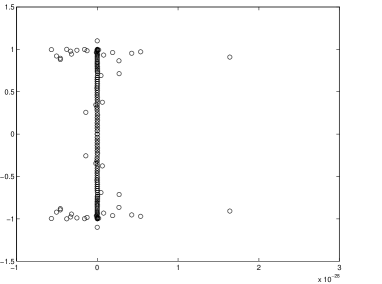
      Figure 5: Scheme $2b$

   3. A staggered grid discretization based on the variables $u_{i}=u(t,ih)$, $v_{i+1/2}=v(t,ih+h/2)$ (see Fig. 6)

      $$\dot{u}_{i}=\frac{v_{i+1/2}-v_{i-1/2}}{h}+\frac{v_{i+1/2}+v_{i-1/2}}{2ih},\quad\dot{v}_{i+1/2}=\frac{u_{i+1}-u_{i}}{h}.$$

      

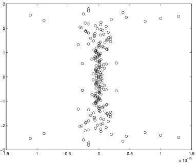
      Figure 6: Scheme $2c$

   Again, we find that discretizing in a centered and compatible way yields a purely imaginary spectrum (again up to round-off error). The staggering in scheme $2c$ is suggested by the structure of the equations which is ultimately related to the meaning of the variables. While $u$ is a time derivative located at the grid points $v$ is a spatial derivative which should be located between the grid points.

3. The final three discretization schemes of (12) are somewhat different from the ones above:

   1. This scheme takes the idea of centering to fourth order and again yields a purely imaginary spectrum (see Fig. 7)

      $$\dot{u}_{i}=\frac{v_{i-2}-8v_{i-1}+8v_{i+1}-v_{i+2}}{12h}+\frac{-v_{i-2}+4v_{i-1}+4v_{i+1}-v_{i+2}}{6ih}.$$

      

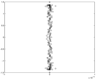
      Figure 7: A fourth order centered scheme, $3a$

   2. The next scheme makes use of further information coming from the theory of group actions. While the radial coordinate $r$ is not a smooth coordinate on the orbit space its square is smooth. Hence, it seems natural to express the variables as functions of the coordinate $x=r^{2}$. Then the minor redefinition $\tilde{u}(x)=2u(r)$ and $\tilde{v}(x)=rv(r)$ of the variables yields the (regular) system

      $$\partial_{t}{\tilde{u}}=\partial_{x}\tilde{v},\qquad\partial_{t}{\tilde{v}}=x\partial_{x}\tilde{u},$$

      which is discretized in the standard way (see Fig. 8)

      $$\dot{\tilde{u}}_{i}=\frac{\tilde{v}_{i+1}-\tilde{v}_{i-1}}{2h},\qquad\dot{\tilde{v}}_{i}=\frac{i}{2}(\tilde{u}_{i+1}-\tilde{u}_{i-1}).$$

      

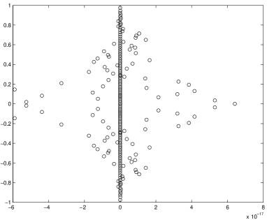
      Figure 8: Standard discretization for redefined system

   3. The same system discretized using a staggered grid (see Fig. 9)

      $$\dot{\tilde{u}}_{i}=\frac{\tilde{v}_{i+1/2}-\tilde{v}_{i-1/2}}{h},\qquad\dot{\tilde{v}}_{i+1/2}=(i+1/2)(\tilde{u}_{i}-\tilde{u}_{i-1}).$$

      

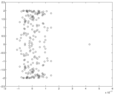
      Figure 9: Staggered discretization for redefined system

V Conclusion

We discussed in this work several schemes for treating axisymmetric systems which are difficult to handle numerically due to the degenarcy of adapted coordinates and hence the formal singularity of the ensuing equations. We applied various schemes to the axisymmetric wave equation written as a symmetric hyperbolic system for the derivatives and determined the spectrum of the ensuing matrices. As a consequence of the shape of the stability regions of common ODE solvers we take the appearance of handles and outliers described in section IV as an indication for a ‘bad’ discretization scheme. These eigenvalues correspond to grid modes which, when evolved with a standard ODE solver, will lead to instabilities. In order to avoid them one needs to be careful in discretizing the equations because the derivative term and the $1/x$ term must be treated in a compatible way. This is due to their common geometric origin. In the general case, where tensors of higher rank are involved different terms may have to be combined. Exactly which terms these are is indicated by the behaviour of the tensor components under the symmetry transformation.

One particular method we discussed is the cartoon method. It turns out that this method is not really different from a direct implementation of the axisymmetry in terms of the adapted coordinates. Here the problem is to make the interpolation compatible with the discretization in the $y=0$ half plane so that parasitic modes are excluded. However, the advantage in using the cartoon method is that it admits a quick and easy extension of a 2D axisymmetric code to a full 3D code because the underlying grid structure and the equations need not be changed.

Clearly, this investigation cannot deliver the ultimate solution to the problem. It should be regarded as providing a guide to eliminate ‘bad’ discretizations and suggesting possible ‘good’ ones. For instance, we have implemented the schemes $1c$ and $3a$ in our axisymmetric code Frauendiener and Hein (2002) for solving the conformal field equations. While these schemes perform well for the axisymmetric wave equation they still tend to produce slowly growing instabilities in the case of the quasilinear conformal field equations. This behaviour might be related to the fact that in most cases the real parts of the eigenvalues vanish only up to round-off error and that these small real parts start to grow due to non-linear interactions. It would be useful to have a scheme in which the spectrum is exactly on the imaginary axis and whose only non-vanishing eigenvalues are the physical ones. However, such a scheme is probably impossible to find.

Appendix A Stability regions

We illustrate the procedure for determining the stability region of a particular time evolution scheme for an explicit Runge-Kutta scheme. Let $\dot{u}=f(t,u)$ be the (system of) ODE(s) which we intend to solve. An explicit Runge-Kutta scheme with $s$ ‘stages’ to compute an approximation $u_{1}$ of $u(t_{0}+h)$ is formulated as follows:

$$k_{1} =f(t_{0},u_{0}),$$

$$k_{2} =f(t_{0}+c_{2}h,u_{0}+ha_{21}k_{1}),$$

$$k_{3} =f(t_{0}+c_{3}h,u_{0}+ha_{31}k_{1}+ha_{32}k_{2}),$$

$$\cdots$$

$$k_{s} =f(t_{0}+c_{s}h,u_{0}+ha_{s1}k_{1}+ha_{s2}k_{2}+\cdots+ha_{ss-1}k_{s-1}),$$

$$u_{1} =u_{0}+h(b_{1}k_{1}+\cdots+b_{s}k_{s}).$$

The particular scheme is characterized entirely by the coefficients $a_{ik}$, $b_{i}$ and $c_{k}$ which are conveniently presented as a tableau

$$\begin{array}[]{c|ccccc}0&&&&&\\ c_{2}&a_{21}&&&&\\ c_{3}&a_{31}&a_{32}&&&\\ \vdots&\vdots&\vdots&\ddots&&\\ c_{s}&a_{s1}&a_{s2}&\cdots&a_{ss-1}&\\ \hline\cr&b_{1}&b_{2}&\cdots&b_{s-1}&b_{s}\end{array}$$

The method is said to be of $p$-th order if for sufficiently smooth $f$ the condition

$$||u_{1}-u(t_{0}+h)||\leq Ch^{p+1}$$

holds.

To get to the stability region one applies the scheme to the specific model equation $\dot{u}=\lambda u$ where $\lambda\in{\mathbb{C}}$ is arbitrary. Going through the procedure above it is clear that the final result is of the form

$$u_{1}=P(\lambda h)u_{0}$$

where $P(z)$ is a polynomial of degree $s$, the so called stability function of the method. Since $||u_{1}||=|P(\lambda h)|\;||u_{0}||$ we find that the method will produce bounded approximations if and only if $|P(\lambda h)|\leq 1$. This motivates the definition of the stability region as the set

$$\Omega=\{z\in{\mathbb{C}}\bigm{|}\;|P(z)|\leq 1\}.$$

In case of an implicit scheme the stability function, obtained in the same way by applying the scheme to the model equation, is not a polynomial but a rational function. In a similar way, the stability regions of linear multistep schemes are obtained. Here, the simplest one is the leapfrog scheme which updates $u_{n+1}$ from the values on the previous time levels $u_{n}$ and $u_{n-1}$ as $u_{n+1}=u_{n-1}+2hf(t_{0}+nh,u_{n})$. It is easy to see that the stability region for the leapfrog scheme is the part of the imaginary axis between $-\mathrm{i}$ and $\mathrm{i}$.

The stability regions for explicit Runge-Kutta schemes of order $p=s$ for $s=1,2,3,4$ are shown in Fig. 10.

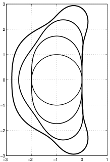
Figure 10: Stability regions for explicit Runge-Kutta schemes with $p=s$

The stability regions for the second and third order Adams-Bashforth methods are shown in Fig. 11

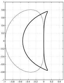
Figure 11: Stability regions for second (thin line) and third (thick line) order Adams-Bashforth methods

as an example for stability regions of multistep methods. For the stability regions of other multistep schemes we refer to Fornberg (1996); Gustafsson et al. (1995). Qualitatively, these regions extend into the left half plane of the complex plane including possibly some part of the imaginary axis. For higher order methods the stability region may even extend into the right half plane.

Appendix B The ICN time evolution scheme

The ICN scheme was described in Teukolsky (2000) in application to a one-dimensional advection equation. Viewing the ICN scheme as a time stepper to solve systems of ODEs $\dot{u}=f(t,u)$ one can deduce from this description the following algorithm to compute $u_{1}\approx u(t_{0}+h)$

$$k_{1} =f(t_{0},u_{0}),$$

$$k_{2} =f(t_{0}+\tfrac{1}{2}h,u_{0}+\tfrac{1}{2}hk_{1}),$$

$$k_{3} =f(t_{0}+\tfrac{1}{2}h,u_{0}+\tfrac{1}{2}hk_{2}),$$

$$\cdots$$

$$k_{s} =f(t_{0}+\tfrac{1}{2}h,u_{0}+\tfrac{1}{2}hk_{s-1}),$$

$$u_{1} =u_{0}+hk_{s}.$$

Cleary, this is an explicit Runge-Kutta scheme with the tableau

$$\begin{array}[]{c|ccccc}0&&&&&\\ \tfrac{1}{2}&\tfrac{1}{2}&&&&\\ \tfrac{1}{2}&0&\tfrac{1}{2}&&&\\ \vdots&\vdots&\vdots&\ddots&&\\ \tfrac{1}{2}&0&0&\cdots&\tfrac{1}{2}&\\[5.0pt] \hline\cr&0&0&\cdots&0&1.\end{array}$$

Note, that $k$ iterations correspond to $s=k+1$ stages of the corresponding Runge-Kutta scheme. Application of this scheme to the model equation $\dot{u}=\lambda u$ yields the stability function

$$P_{s}(z)=1+z\sum_{k=0}^{s-1}\left(\frac{z}{2}\right)^{k}=1+z+\frac{z^{2}}{2}+\frac{z^{3}}{4}\sum_{k=0}^{s-3}\left(\frac{z}{2}\right)^{k}.$$

The fact that the first three terms agree with the Taylor expansion of $\exp(z)$, the stability function of the exact time evolution, shows that this scheme is second order accurate Hairer et al. (2000). The stability regions are obtained as the level set $\{P_{s}(z)P_{s}(\bar{z})=1\}$. The regions for some values of $s$ are shown in Fig. 12.

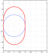
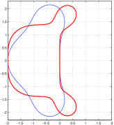
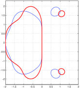
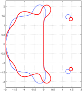
Figure 12: The stability regions for ICN(s) for $s=1,2$, $s=3,4$, $s=5,6$ and $s=7,8$

We see that the imaginary axis intersects the stability regions for $s=3,4,7,8,\ldots$ in a finite interval while for the other values they have only the origin in common with the imaginary axis. To explain this somewhat unexpected result we look at the behaviour of the modulus of the stability function on the imaginary axis in a neighbourhood of the origin. Writing

$$P_{s}(z)=1+z\sum_{k=0}^{s-1}\left(\frac{z}{2}\right)^{k}=1+z\frac{1-\left(\frac{z}{2}\right)^{s}}{1-\frac{z}{2}}$$

and inserting $z=\mathrm{i}y$ into $Q(z)=P_{s}(z)P_{s}(\bar{z})$ we find

$$Q(\mathrm{i}y)=1+2\frac{-(\mathrm{i}y/2)^{s+1}(1+(-1)^{s+1})+(\mathrm{i}y/2)^{s+2}(1+(-1)^{s})+2(y/2)^{2s+2}}{1+(y/2)^{2}}.$$

This shows that for all $s>1$

$$Q(\mathrm{i}y)=\begin{cases}1-\left(\frac{\displaystyle\mathrm{i}}{\displaystyle 2}\right)^{s}\,y^{s+2}+\cdots&s\text{ even}\\ 1+\left(\frac{\displaystyle\mathrm{i}}{\displaystyle 2}\right)^{s+1}\,y^{s+1}+\cdots&s\text{ odd}.\end{cases}$$

The behaviour of the stability regions is determined by the coefficient of the lowest order term. These lead to the sequence $1$, $1/4$, $-1/4$, $-1/16$, $1/16$, $\dots$ for $s=1,2,\ldots$. The negative coefficients imply a decrease of $Q(iy)$ along the imaginary axis close to $y=0$ and hence they correspond to the cases where the stability region contains a part of the imaginary axis. The other cases, when the coefficient of the dominating term is positive, are those when the stability region just touches the imaginary axis at the origin. In these cases, systems with eigenvalues on or to the right of the imaginary axis such as in particular the advection equation and other hyperbolic equations cannot be stably evolved with ICN. Thus, we come to the same conclusion as in Teukolsky (2000), namely that ICN($k$) for $k=2,3,6,7,\ldots$ is unstable for hyperbolic equations. Furthermore, since the method is always second order accurate regardless of how many iterations are performed, there is no use in performing more than two. In fact, in most practical cases it is probably more efficient to use a higher order Runge-Kutta method instead.

Another interesting aspect of the ICN scheme is its relationship with the Crank-Nicholson method. This is a second order accurate, implicit time stepping scheme whose stability function is given by

$$P(z)=\frac{1+z/2}{1-z/2}$$

and whose stability region is the entire left plane. Taking the limit of $P_{s}(z)$ for $s\to\infty$ we find that in fact $P_{s}(z)\to P(z)$. However, absolute convergence holds only in the circle $|z|<2$. This has the following implication: iterating the ICN scheme until convergence to produce approximations to the exact Crank-Nicholson method works only within that circle. Thus, this scheme (which might be termed ‘the full ICN scheme’) also has a stability barrier and hence a limitation of the time step in contrast to the exact CN scheme which is unconditionally stable. Thus, we conclude that the ICN scheme is not an efficient alternative to higher order Runge-Kutta or implicit schemes like CN.

References

- Alcubierre et al. (1999) M. Alcubierre, S. Brandt, B. Brügmann, D. Holz, E. Seidel, R. Takahashi, and J. Thornburg, Phys. Rev. D (1999).
- Frauendiener and Hein (2002) J. Frauendiener and M. Hein (2002), in preparation.
- Jänich (1968) K. Jänich, Differenzierbare -Mannigfaltigkeiten, vol. 59 of Lecture Notes in Mathematics (Springer-Verlag, Heidelberg, 1968).
- Frauendiener (1987) J. Frauendiener, Ph.D. thesis, Universität Tübingen (1987).
- Thornburgh (2002) J. Thornburgh, private communication.
- Teukolsky (2000) S. A. Teukolsky, Phys. Rev. D 61, 087501 (2000).
- Hairer et al. (2000) E. Hairer, S. P. Nørsett, and G. Wanner, Solving Ordinary Differential Equations, vol. I (Springer-Verlag, Berlin, 2000), 2nd ed.
- Hairer and Wanner (1996) E. Hairer and G. Wanner, Solving Ordinary Differential Equations, vol. II (Springer-Verlag, Berlin, 1996), 2nd ed.
- Trefethen (2000) L. N. Trefethen, Spectral methods in Matlab (SIAM, Philadelphia, 2000).
- Fornberg (1996) B. Fornberg, A practical guide to pseudospectral methods (Cambridge University Press, Cambridge, 1996).
- Gustafsson et al. (1995) B. Gustafsson, H.-O. Kreiss, and J. Oliger, Time dependent problems and difference methods (Wiley, New York, 1995).