Black Hole Interaction Energy

Abstract

The interaction energy between two black holes at large separation distance is calculated. The first term in the expansion corresponds to the Newtonian interaction between the masses. The second term corresponds to the spin-spin interaction. The calculation is based on the interaction energy defined on the two black holes initial data. No test particle approximation is used. The relation between this formula and cosmic censorship is discussed.

1 Introduction

The purpose of this article is to prove, under appropriate assumptions, the following statement: the interaction energy, at large separation distance $l$, between two black holes of masses $M_{1}$, $M_{2}$ and spins $J_{1}$, $J_{2}$ is given by

$$E=\frac{-M_{1}M_{2}}{l}+\frac{-J_{1}\cdot J_{2}+3(J_{1}\cdot\hat{n})(J_{2}\cdot\hat{n})}{l^{3}}+\text{ higher order terms},$$ (1)

where $\hat{n}$ is a unit vector which points inward along the line connecting the black holes. Before giving a precise definition of the parameters involved in Eq. (1), I want to discuss its physical meaning.

The first term in Eq. (1) has the Newtonian form. For two point particles of masses $M_{1}$ and $M_{2}$ separated by an Euclidean distance $l$, the Newtonian interaction energy between them is given by $-M_{1}M_{2}/l$. The fact that this term appears also for a two black holes system in General Relativity can be expected from the weak field limit of Einstein’s equations. The second term in Eq. (1), which involves the spins, has analogous form to the dipole-dipole electromagnetic interaction; there exists an analogy between magnetic dipole in electromagnetism and spin in general relativity (see [35]). In the electromagnetic case, $l$ is the Euclidean distance between two charge distributions and $J_{1}$, $J_{2}$ the corresponding dipole moments of them. However, the gravitational black hole spin-spin interaction has the opposite sign to the electromagnetic one. The first evidence of this fact was given by Hawking [25]. I want to reproduce Hawking’s argument here because it points out the connection between Eq. (1) and the cosmic censorship conjecture (see also the discussion in [35]). In the argument, we assume the following two consequences of weak cosmic censorship and the theory of black holes (cf. [27] [37], see also [36]):

• Every apparent horizon must be entirely contained within the black hole event horizon.

• If matter satisfies the null energy condition (i.e. if $T_{ab}k^{a}k^{b}\geq 0$ for all null $k^{a}$), then the area of the event horizon of a black hole cannot decrease in time.

We also assume:

• All black holes eventually settle down to a final Kerr black hole.

Consider a system of two black holes such that, at a given time, the separation distance between them is large. Then, there must exist a Cauchy surface in the asymptotically flat region of the space time such that the intersection of the hypersurface with the event horizon has two disconnected component of areas $A_{1}$ and $A_{2}$. Since the black holes are far apart, these areas can be approximated by the Kerr formula

$$A_{1}=8\pi\left(M^{2}_{1}+\sqrt{M_{1}^{4}-J_{1}^{2}}\right),\quad A_{2}=8\pi\left(M^{2}_{2}+\sqrt{M_{2}^{4}-J_{2}^{2}}\right).$$ (2)

At late times, after the collision, the system will settle down to a Kerr black hole. Hence, there must exist another Cauchy hypersurface such that its intersection with the event horizon will have area

$$A_{f}=8\pi\left(M^{2}_{f}+\sqrt{M_{f}^{4}-J_{f}^{2}}\right),$$ (3)

where $M_{f}$ is mass of the final black hole and $J_{f}$ is its final angular momentum. By (ii) we have

$$A_{f}\geq A_{1}+A_{2}.$$ (4)

Since gravitational waves have positive mass, we also have

$$M_{f}\leq M_{1}+M_{2}.$$ (5)

In general, gravitational waves will carry angular momentum. But in axially symmetric space-times the total angular momentum is a conserved quantity, since it can be defined by a Komar integral (cf. [28] and also [37]). Then, in this case we have

$$J_{f}=J_{1}+J_{2}.$$ (6)

Using Eqs. (2), (3), (4) and (6) it is possible to obtain an upper bound, which depends on $J_{1}$ and $J_{2}$, to the total amount of radiation emitted by the system $M_{1}+M_{2}-M_{f}$. It can be seen that if $J_{1}$ and $J_{2}$ have the same sign, this upper bound is smaller than if they have opposite sign. This suggests that there may be a spin-spin force between the black holes that is attractive if the angular momentum have opposite directions and repulsive if they have the same direction. Presumably, in the second case the system expends energy in doing work against the spin repulsive force, and for this reason this energy is not available to be radiated via gravitational radiation.

Hawking’s argument only suggests that the spin interaction energy between black holes has in fact this sign dependence with respect to the spins. It is not a proof, first because there is no proof for the weak cosmic censorship conjecture (i)-(ii) and for the assumption (iii). Second, because even if we assume (i)–(iii) the argument only shows that an upper bound of the total amount of radiated energy has this sign dependence in terms of $J_{1}$ and $J_{2}$, but the real amount of gravitational radiation can, in principle, have other dependence. In fact, the total amount of gravitational radiation produced by such systems, as numerical studies show, is much smaller than this bound. This upper bound is $50\%$ of the total mass when the spins are antiparallel, the black holes are extreme ($J^{2}=M$), and have equal masses; when the spins are zero or when the black holes are extreme with parallel spins, the upper bound is $29\%$ of the total mass. On the other hand, in the numerical calculations the maximum amount of radiation emitted by this type of system is about $3\%$ of the total mass, see [2] [3] for a recent calculation and also [29] for an up to date review on the subject. However, the numerical studies show that the system indeed radiates less when the spins are parallel than when they are antiparallel. Moreover, Wald [35] proves that the interaction energy between a test particle with spin $J_{2}$ and a stationary background of spin $J_{1}$ has precisely this sign dependence. Wald shows that the spin-spin interaction energy has the form

$$\frac{-J_{1}\cdot J_{2}+3(J_{1}\cdot\hat{n})(J_{1}\cdot\hat{n})}{l^{3}},$$ (7)

where $l$ and $\hat{n}$ are defined as follows. The stationary field is expanded at large distance with respect to Cartesian asymptotic coordinates $x^{i}$, here $l$ is the Euclidean radius with respect to $x^{i}$ and $\hat{n}^{i}=x^{i}/l$. Eq. (7) has been also proved by D’Eath using post-Newtonian expansions [18]. It is important to note that Eq. (7) gives an indirect evidence in support of (i)-(iii).

In this article I want to prove Eq. (7) without using either the particle or post-newtonian approximation. The proof is based on an interaction energy defined on the two black hole initial data. This interaction energy is genuinely non linear; it does not involve any approximation.

The plan of the paper is as follows. In section 2 the main results are given. In section 3 theorem 2.2 is proved; in section 4 we prove corollary 2.3. Finally, in section 5 an alternative definition of the interaction energy is discussed.

2 Main Result

The strategy I will follow was given by Brill and Lindquist [10]. It is based on the analysis of initial data set with many asymptotic ends. An initial data set for the Einstein vacuum equations is given by a triple $(\tilde{S},\tilde{h}_{ab},\tilde{K}_{ab})$ where $\tilde{S}$ is a connected 3-dimensional manifold, $\tilde{h}_{ab}$ a (positive definite) Riemannian metric, and $\tilde{K}_{ab}$ a symmetric tensor field on $\tilde{S}$. They satisfy the vacuum constraint equations

$$\tilde{D}^{b}\tilde{K}_{ab}-\tilde{D}_{a}\tilde{K}=0,$$ (8)

$$\tilde{R}+\tilde{K}^{2}-\tilde{K}_{ab}\tilde{K}^{ab}=0,$$ (9)

on $\tilde{S}$, where $\tilde{D}_{a}$ is the covariant derivative with respect to $\tilde{h}_{ab}$, $\tilde{R}$ is the trace of the corresponding Ricci tensor, $\tilde{K}=\tilde{h}^{ab}\tilde{K}_{ab}$, and $a,b,c...$ denote abstract indices. Tensor indices of quantities with tilde will be moved with the metric $\tilde{h}_{ab}$ and its inverse $\tilde{h}^{ab}$. The data will be called asymptotically flat with $N+1$ asymptotic ends, if for some compact set $\Omega$ we have that $\tilde{S}\setminus\Omega=\sum_{k=0}^{N}\tilde{S}_{k}$, where $\tilde{S}_{k}$ are open sets such that each $\tilde{S}_{k}$ can be mapped by a coordinate system $x^{j}$ diffeomorphically onto the complement of a closed ball in $\mathbb{R}^{3}$ such that we have in these coordinates

$$\tilde{h}_{ij}=(1+\frac{2M_{k}}{r})\delta_{ij}+O(r^{-2}),$$ (10)

$$\tilde{K}_{ij}=O(r^{-2}),$$ (11)

as $r=(\sum_{j=1}^{3}({x^{j}})^{2})^{1/2}\to\infty$ in each set $\tilde{S}_{k}$; where $i,j\cdots$, which take values $1,2,3$, denote coordinates indices with respect to the given coordinate system $x^{j}$, and $\delta_{ij}$ denotes the flat metric. We will call the coordinate system $x^{i}$ an asymptotic coordinate system at the end $k$. Each asymptotic region $\tilde{S}_{k}$ has a different asymptotic coordinate system. The constant $M_{k}$ denotes the ADM mass[1] of the data at the end $k$. These conditions guarantee that the mass, the linear momentum, and the angular momentum of the initial data set are well defined at every end.

For $N\geq 1$, this class of data contains, in general, apparent horizons. The existence of apparent horizons leads us to interpret these data as representing initial data for black-holes. Their evolution will presumably contain an event horizon, according to the standard theory of black holes [27]. The validity of this picture depends, of course, on the cosmic censorship conjecture. The only statement about the evolution of the data that we can make is the geodesic incompleteness of the space time. In general, in order to prove the geodesic incompleteness of a space time, one needs to know that the data contain a trapped surface in order to apply the singularities theorems [27]. However, in this particular case, since the topology of the data is not trivial, the geodesic incompleteness of the space time follows directly from a theorem proved by Gannon [22].

For simplicity we will fix $N=2$, see Fig. 1.

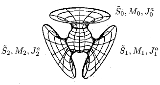
Figure 1: Initial data with three asymptotic ends ($N=2$). For each asymptotic region $\tilde{S}_{k}$, we have the corresponding mass $M_{k}$ and total angular momentum $J^{a}_{k}$.

In this case the data can be interpreted as initial data with two black holes. This interpretation is suggested by the following fact: when an appropriate distance parameter is large compared with the masses $M_{k}$, then it can be seen numerically that only two disconnected apparent horizons appear. For time symmetric data, these numeric calculations have been done in [10]; the non-time symmetric case has been studied by Cook (see [14] and references therein). It is not clear that the number of apparent horizons is the number of black holes contained in the data, since even when there are two disconnected apparent horizons, the intersection of the event horizon with the initial data can be connected. However, at large separation distance, this seems to be a reasonable assumption, which is confirmed by the numerical evolutions [29].

Brill and Lindquist define the following interaction energy at the end $k$

$$E_{k}=M_{k}-\sum^{N}_{\begin{subarray}{c}k^{\prime}=0\\ k^{\prime}\neq k\end{subarray}}M_{{k^{\prime}}}.$$ (12)

The energy $E_{k}$ is a geometric quantity; its definition does not involves any approximation. The question now is how to calculate $E_{k}$ in terms of physically relevant parameters. The first problem is how to define an appropriate separation distance between the black holes. When there are two apparent horizons, there is a well defined separation distance $l_{\tilde{h}}$ defined as the minimum geodesic distance between any two points in the two different horizons, see Fig. 2.

Figure 2: An initial data set with three asymptotic end points and only two disconnected apparent horizons of area $A_{1}$, $A_{2}$, and radii $R_{1}$, $R_{2}$. The points $i_{1}$ and $i_{2}$ represent the two other infinities $1$ and $2$. The geodesic distance $l_{\tilde{h}}$ is computed with the physical metric $\tilde{h}_{ab}$. The parameter $l$ is computed with the conformal metric. The geodesic distance between $i_{1}$ and $i_{2}$ with respect to the physical metric is infinite.

However, the distance $l_{\tilde{h}}$ is hard to compute. The location of the apparent horizons can be calculated only numerically. Since we are only interested in the energy at large separations, instead of $l_{\tilde{h}}$ we will use another parameter $l$, and we will argue that $l_{\tilde{h}}\approx l$ in this limit. The definition of the parameter $l$ is related to the way in which one can construct solutions of the constraint equations with many asymptotic ends. The conformal method (cf. [11], [12] and the references therein) is a general method for constructing solutions of the constraint equations. We assume that $h_{ab}$ is a positive definite metric with covariant derivative $D_{a}$, and $K^{ab}$ is a trace-free (with respect to $h_{ab}$), symmetric tensor, satisfying

$$D_{a}K^{ab}=0\quad\mbox{on}\quad\tilde{S}.$$ (13)

Let $\varphi$ be a solution of

$$L_{h}\varphi=-\frac{1}{8}K_{ab}K^{ab}\varphi^{-7}\quad\mbox{on}\quad\tilde{S},$$ (14)

where $L_{h}=D^{a}D_{a}-R/8$ and $R$ is the scalar curvature of the metric $h_{ab}$. Then the physical fields $(\tilde{h},\tilde{K})$ defined by $\tilde{h}_{ab}=\varphi^{4}h_{ab}$ and $\tilde{K}^{ab}=\varphi^{-10}K^{ab}$ will satisfy the vacuum constraint equations on $\tilde{S}$. We have assumed that $K^{ab}$ is trace-free; hence $\tilde{K}^{ab}$ will be also trace-free with respect to $\tilde{h}_{ab}$. That is, the initial data set will be maximal.

To ensure asymptotic flatness of the data at the each end $k$, we will require the following boundary conditions. Let $i_{1}$ and $i_{2}$ be two, arbitrary points in $\mathbb{R}^{3}$, with coordinates $x_{1}^{j}$ and $x_{2}^{j}$ in some Cartesian coordinate system $x^{i}$. Define the manifold $\tilde{S}$ by $\tilde{S}=\mathbb{R}^{3}\setminus\{i_{1},i_{2}\}$. Assume that $h_{ab}$ is regular on $\mathbb{R}^{3}$. At infinity we will impose the following fall off behavior

$$h_{ij}=\delta_{ij}+O(r^{-2}),$$ (15)

$$K^{ab}=O(r^{-2}),$$ (16)

$$\varphi=1+O(r^{-1}).$$ (17)

At the points $i_{1}$ and $i_{2}$ we require

$$K^{ab}=O(r_{1}^{-4}),\quad K^{ab}=O(r_{2}^{-4}),$$ (18)

where

$$r_{1}=\left(\sum_{i=1}^{3}(x^{i}-x_{1}^{i})^{2}\right)^{1/2},\quad r_{2}=\left(\sum_{i=1}^{3}(x^{i}-x_{2}^{i})^{2}\right)^{1/2},$$ (19)

and

$$\lim_{r_{1}\rightarrow 0}r_{1}\varphi=\frac{m_{1}}{2},\quad\lim_{r_{2}\rightarrow 0}r_{2}\varphi=\frac{m_{2}}{2},$$ (20)

where $m_{1}$ and $m_{2}$ are positive constants. Note that both $\varphi$ and $K^{ab}$ are singular at $i_{1}$, $i_{2}$.

One can prove that the data so constructed will be asymptotically flat at the three ends. We have made an artificial distinction between the end $0$, given by $r\rightarrow\infty$, and the ends $1$ and $2$. It is possible to discuss the same construction in a more geometrical way, such that all ends are treated equally; see [5], [20], [21], [15]. However, since our final goal is to calculate the interaction energy at one end, it is convenient to make this distinction. The coordinate system $x^{i}$ and the corresponding flat metric in the expansion Eq. (15), gives the Euclidean distance $l$ between $i_{1}$ and $i_{2}$

$$l=\left(\sum_{i=1}^{3}(x_{2}^{i}-x_{1}^{i})^{2}\right)^{1/2},$$ (21)

which will be our separation distance parameter, see Fig. 2.

In general, Eq. (14) is non-linear. However if we assume that the data is time symmetric, i.e. $K^{ab}=0$, then it becomes a linear equation for $\varphi$. If we assume that the conformal metric is flat, we obtain a Laplace equation for $\varphi$. The solution of this equation that satisfies the boundary conditions Eqs. (20) and (17) is given by

$$\varphi_{0}=1+\frac{m_{1}}{2r_{1}}+\frac{m_{2}}{2r_{2}}.$$ (22)

This solution was found by Brill and Lindquist in [10]. In this case it is possible to calculate explicitly the interaction energy (12) in terms of the masses and the separation distance. The result is the following.

Theorem 2.1 (Brill-Lindquist)

Let $h_{ab}$ the flat metric and $\tilde{K}^{ab}=0$. Then the interaction energy defined by Eq. (12) is always negative. Moreover, when $l$ is large compared with $M_{k}$ the following expansion holds

$$E_{0}=-\frac{M_{1}M_{2}}{l}+\text{ higher order terms}.$$ (23)

Giulini [24] has computed the higher order terms for these data and other conformally flat time symmetric data with different topologies. In those examples the Newtonian term is invariant but the higher order terms depend on the particular initial data.

In order to discuss spin-spin interaction, we need initial data with non trivial angular momentum, that is we have to allow for non trivial extrinsic curvature in the data. At each end we have the angular momentum $J_{k}$ given by

$$J_{k}^{a}=\frac{1}{8\pi}\lim_{r\to\infty}\int_{S_{r}}\,rK_{bc}\,n^{b}\epsilon^{cad}\,n_{d}\,dS_{r},$$ (24)

where $S_{r}$ is a two sphere defined in the asymptotic region $\tilde{S}_{k}$ and $n^{a}$ is its outward unit normal vector. In Eq. (24) we can use either $K^{ab}$ or $\tilde{K}^{ab}$ because the conformal factor satisfies (17). In general the angular momentum at each end is not determined by the intrinsic angular momentum of each black hole. It includes also the angular momentum of the gravitational field surrounding the black holes. Then, in general, there is no relations between $J_{0}$, $J_{1}$ and $J_{2}$, these three quantities can be freely prescribed. But in the presence of symmetries these quantities can not be given freely any more. Moreover, in the presence of conformal symmetries of the metric there exists a well defined quasilocal definition of angular momentum. Assume that $\xi^{a}$ is a conformal Killing vector; that is, a solution of the equation $(\mathcal{L}_{h}\xi)^{ab}=0$, where

$$(\mathcal{L}_{h}\xi)^{ab}=D^{a}\xi^{b}+D^{b}\xi^{a}-\frac{2}{3}\,h^{ab}\,D_{c}\xi^{c}.$$ (25)

If the initial data is maximal, i.e., $K=0$, then the vector $K^{ab}\xi_{b}$ is divergence free. Hence, for each conformal symmetry $\xi^{a}$ we have the associated integral

$$I_{\xi}=\int_{S}K^{ab}\xi_{b}n_{a}dS,$$ (26)

where $S$ is a close 2-surface and $n^{a}$ its outward unit normal vector. This integral is a conformal invariant. It can be calculated also in terms of tilde quantities. The integral (26) will be non zero only if the vector $K^{ab}\xi_{b}$ is singular at some points; in our case it will be singular at two points: the location of the holes. Then the integral in Eq. (26) will have three different values depending on whether the surface $S$ encloses one hole, two holes or no hole. In the later case, $I_{\xi}=0$. If we chose $\xi^{a}$ to be a rotation, $I_{\xi}$ will gives the corresponding component of the quasilocal angular momentum. If the data is conformally flat we have $10$ conformal Killing vectors. In particular, we have the three rotations and hence the complete definition of quasilocal angular momentum. These quantities will be defined only on this slice and will generally not be preserved in the evolution. They will be only preserved if the space time admits a Killing vector. In this case they will coincide with the corresponding Komar integral. The space time will admit a Killing vector field if $\xi^{a}$ is a Killing vector for the whole initial data; that is, $\pounds_{\xi}\tilde{h}_{ab}=\pounds_{\xi}\tilde{K}^{ab}=0$, where $\pounds_{\xi}$ is the Lie derivative with respect to $\xi^{a}$. A conformally flat, maximal, slice can be interpreted as a instant of time in which the gravitational field carries no angular momentum and no linear momentum itself, and hence these quantities are carried only by the “sources”, which in this case are the black holes. Data containing matter with compact support can be also constructed.

There exist in the literature other definitions of quasilocal angular momentum ([33] [30] [19][34]), which are applicable for an arbitrary closed 2-surfaces in the spacetime. It is not clear if any of these definitions will agree with Eq. (26) in the particular case of 2-surface lying on a conformally flat 3-hypersurface.

From the discussion above, we conclude that in the case of conformally flat, maximal data we have,

$$J^{a}_{0}+J^{a}_{1}+J^{a}_{2}=0.$$ (27)

For an observer placed in the asymptotic end $0$ the system will look like two black hole with spins $-J^{a}_{1}$ and $-J^{a}_{2}$, and the total angular momentum will be $J^{a}_{0}=-J^{a}_{1}-J^{a}_{2}$. For a more general discussion of conformal symmetries on initial data see [6] and [17]; in particular in those articles a generalization of Eq. (27) which includes linear momentum is proved.

Bowen and York obtain a simple model for a conformally flat data set which represents two black holes with spins [8]. Brandt and Brügmann [9] study these data with the $N+1$ asymptotic ends boundary conditions given by Eqs. (18), (16), (20) and (17). For these data, the conformal second fundamental form is given by

$$K^{ab}=K_{1}^{ab}+K_{2}^{ab},$$ (28)

where

$$K_{1}^{ab}=\frac{6}{r_{1}^{3}}n_{1}^{(a}\epsilon^{b)cd}J_{1\,c}n_{1\,d},\quad K_{2}^{ab}=\frac{6}{r_{2}^{3}}n_{2}^{(a}\epsilon^{b)cd}J_{2\,c}n_{2\,d},$$ (29)

and

$$n_{1}^{i}=\frac{x^{i}-x_{1}^{i}}{r_{1}},\quad n_{2}^{i}=\frac{x^{i}-x_{2}^{i}}{r_{2}},$$ (30)

where $J_{1}^{c}$, $J_{2}^{c}$ are constants and $\epsilon^{bcd}$ is the flat volume element. One can check that the constants $J_{1}^{c}$ and $J_{2}^{c}$ give the the angular momentum at the ends $1$ and $2$ respectively. The tensors (29) are divergence free and trace free with respect to the flat metric in $\mathbb{R}^{3}\setminus\{i_{1},i_{2}\}$.

The first result of this article is the following theorem.

Theorem 2.2

Let $h_{ab}$ be the flat metric and $K^{ab}$ be given by Eqn. (28). Then, the interaction energy (12) is given by

$$E_{0}=\frac{-M_{1}M_{2}}{l}+\frac{-J_{1}\cdot J_{2}+3(J_{1}\cdot\hat{n})(J_{1}\cdot\hat{n})}{l^{3}}+\text{ higher order terms}.$$ (31)

The expansion of the dimensionless quantity $E_{0}/l$ is made in terms of the dimensionless parameters $M_{1}/l$, $M_{2}/l$, $J_{1}/l^{2}$ and $J_{2}/l^{2}$. By higher order terms we mean terms of cubic order in those parameters. We prove Theorem 2.2 in section 3.

Using similar arguments, Gibbons[23][26] has obtained the qualitative sign dependence of the spin-spin interaction for a certain class of axially symmetric, conformally flat, data. Note that in theorem 2.2, the data are non axially symmetric in general, since the spins can point in arbitrary directions. Bonnor [7] has studied the spin-spin interaction using an exact, axially symmetric solution of the Einstein-Maxwell equations, his result also qualitatively agrees with the spin-spin term in Eq. (31).

The Bowen-York data are, of course, very special. The natural question is how to generalize theorem 2.2 for more general data. For general asymptotically flat data with three asymptotic ends we can not even expect to recover the Newtonian interaction term. Take for example a time symmetric initial data with only two ends. Choosing the conformal metric appropriately, one can easily construct data such that the difference $M_{1}-M_{0}$ is arbitrary. That means that we are putting more radiation in one end than in the other. If we add a third end with small mass, the new interaction energy will be dominated by the difference $M_{1}-M_{0}$ and hence will be not related with any Newtonian force. Hence, theorem 2.1 is not true for general asymptotically flat metrics with many asymptotic ends.

The interaction energy defined by (12) can have the meaning of a two black holes interaction energy only if is it possible to distinguish in the data two objects that are similar to the Kerr black hole when the separation distance is large. I will call this class of data two Kerr-like black hole initial data. The existence of these data has been proved in [16] [15]. The following two properties of the Kerr initial data, in the standard Boyer-Lindquist coordinates, are important: i) The data are conformally flat up to order $O(J^{2})$ ii) The leading order term of the second fundamental form is given by the Bowen-York one (29). Then one can expect that Eq. (31) is unchanged in the principal terms for this class of data.

More precisely, a two Kerr-like black hole initial data can be constructed as follows (see [16] and [15] for details). Take a slice of the Kerr metric, with parameters $M_{K_{1}}$ and $J_{1}$, in the standard Boyer-Lindquist coordinates. Choosing the appropriate conformal factor, the conformal metric can be written in the following form

$$h^{K_{1}}_{ab}=\delta_{ab}+h^{R_{1}}_{ab},$$ (32)

where $h^{R_{1}}_{ab}=O(J_{1}^{2})$. In the same way the conformal second fundamental form can be written as

$$K_{K_{1}}^{ab}=K_{1}^{ab}+K^{ab}_{R_{1}},$$ (33)

where $K^{ab}_{R_{1}}=O(J_{1}^{2})$ and $K_{1}^{ab}$ is given by (29). Take another Kerr metric, with parameters $M_{K_{2}}$ and $J_{2}$, and define the following conformal metric

$$h^{KK}_{ab}=\delta_{ab}+h^{R_{1}}_{ab}+h^{R_{2}}_{ab},$$ (34)

and the following conformal second fundamental form

$$K^{ab}_{KK}=\bar{K}_{K_{1}}^{ab}+\bar{K}_{K_{2}}^{ab}+(\mathcal{L}_{h_{KK}}w)^{ab},$$ (35)

where the bar means the trace free part of the tensor with respect to the metric (34) and $w^{a}$ is chosen such that $K^{ab}_{KK}$ is divergence free and trace free with respect to the metric (34). In [16] [15] it has been proved that such vector $w^{a}$ exists and is unique. Using (34) and (35), solve Eq. (14) with the boundary conditions (20) and (17) where

$$m_{1}=\sqrt{M^{2}_{K_{1}}-J^{2}_{1}/M^{2}_{K_{1}}},\quad m_{2}=\sqrt{M^{2}_{K_{2}}-J^{2}_{2}/M^{2}_{K_{2}}}.$$ (36)

The existence of a unique solution has been proved in [16] [15].

If we chose $J^{a}_{1}$ and $J^{a}_{2}$ to point in the same direction, the data will be axially symmetric. In this particular case, we can use the integral (26) to calculate the quasilocal angular momentum of each of the black holes. The result will be $J^{a}_{1}$ and $J^{a}_{2}$. However, in general, this class of data will admit no conformal Killing vector. In this general situation, it is very hard to compute the quasilocal spins of each of the black holes. However, when the separation distance is large, $J^{a}_{1}$ and $J^{a}_{2}$ will give approximately the angular momentum of each of the black holes because this class of data have a far limit to the Kerr initial data. In other words, $J^{a}_{1}$ and $J^{a}_{2}$ give the spins of one black hole when the parameters of the other are set to zero.

For this class of data we have the following result.

Corollary 2.3

For the two Kerr-like data defined above, the formula (31) for the interaction energy holds.

We prove this Corollary in section 4.

3 Interaction Energy for the spinning Bowen-York initial data

In this section we will prove theorem 2.2. For Bowen-York data, with the boundary condition (20) and (17), Eq. (14) for the conformal factor can be written in the following form[9]

$$\Delta u=-\frac{K^{ab}K_{ab}}{8\varphi^{7}},\quad\varphi=\varphi_{0}+u,$$ (37)

with the boundary condition

$$\lim_{r\rightarrow\infty}u=0,$$ (38)

where $\varphi_{0}$ is defined in Eq. (22), with $m_{1}$ and $m_{2}$ arbitrary positives constants, and $K^{ab}=K_{1}^{ab}+K_{2}^{ab}$ is given by (29).

The coordinates $x^{i}$ are asymptotic coordinates for the end $0$. The total mass at $0$ is given by

$$M_{0}=m_{1}+m_{2}+2u_{\infty},$$ (39)

where $u_{\infty}$ is the term which goes like $1/r$ in the solution $u$ of Eq. (37) and is given by

$$u_{\infty}=\frac{1}{4\pi}\int_{\mathbb{R}^{3}}\frac{K^{ab}K_{ab}}{8\varphi^{7}}dx^{3}.$$ (40)

We want to calculate the masses $M_{1}$ and $M_{2}$ for the other ends. The asymptotic coordinates for the other ends are

$$\hat{x}_{i_{1}}^{i}=\frac{m_{1}^{2}}{4}\frac{(x^{i}-x_{1}^{i})}{r_{1}^{2}},\quad\hat{x}_{i_{2}}^{i}=\frac{m_{2}^{2}}{4}\frac{(x^{i}-x_{2}^{i})}{r_{2}^{2}}.$$ (41)

Take for example the end point $i_{1}$, in $\hat{x}_{i_{1}}^{i}$ coordinates we have

$$\tilde{h}_{\hat{i}\hat{j}}=\left(1+\frac{m_{1}}{2\hat{r}_{1}}+\frac{m_{1}m_{2}}{4l\hat{r}_{1}}+\frac{u(i_{1})}{2\hat{r_{1}}}\right)\delta_{\hat{i}\hat{j}}+O(1/\hat{r}^{2}_{1}),$$ (42)

where we have used

$$r_{2}=l+O(1/\hat{r}_{1}),$$ (43)

and $\hat{r}_{1}$ is the Euclidean radius with respect to $\hat{x}_{i_{1}}^{i}$. Then the mass at this end is given by

$$M_{1}=m_{1}\left(1+\frac{m_{2}}{2l}+u(i_{1})\right),$$ (44)

where $u(i_{1})$ denote the value of the function $u$ at the point $i_{1}$. In analogous way we obtain the mass at the end $2$

$$M_{2}=m_{2}\left(1+\frac{m_{1}}{2l}+u(i_{2})\right).$$ (45)

Then the interaction energy at the end $i_{0}$ is given by

$$E_{0}=M_{0}-M_{1}-M_{2}=-\frac{m_{1}m_{2}}{l}+2u_{\infty}-m_{1}u(i_{1})-m_{2}u(i_{2}).$$ (46)

Using Eq. (37) and the Green’s function for the Laplacian, we obtain the following integral representation of the terms involving $u$ in Eq. (46)

$$2u_{\infty}-m_{1}u(i_{1})-m_{2}u(i_{2})=\frac{1}{16\pi}\int_{\mathbb{R}^{3}}\frac{K^{ab}K_{ab}}{\varphi^{7}}\left(1-\frac{m_{1}}{2r_{1}}-\frac{m_{2}}{2r_{2}}\right)dx^{3}.$$ (47)

The formula (47) involves the unknown function $u$. Using the fact that $u$ is $O(J^{2})$, we make an expansion of this integral in terms of the parameters $J_{1}/l^{2}$, $J_{2}/l^{2}$, $m_{1}/l$ and $m_{2}/l$. We obtain that the first non trivial term is given by

$$2u_{\infty}-m_{1}u(i_{1})-m_{2}u(i_{2})\approx E^{s},$$ (48)

where

$$E^{s}=\frac{1}{8\pi}\int_{\mathbb{R}^{3}}K_{1}^{ab}K_{2\,ab}\,dx.$$ (49)

The interaction energy, up to this order, is given by

$$E=-\frac{M_{1}M_{2}}{l}+E^{s},$$ (50)

where we have used Eqs. (44) and (45) to replace $m_{k}$ by $M_{k}$, since up to this order they are equal.

All that remains is to compute the integral $E^{s}$. This integral can, in principle, be calculated explictly from the expressions (29). However such a calculation is very complicated. Instead of this we will calculate (49) in the following way. The tensors (29) can be written like

$${(\mathcal{L}_{\delta}v_{1})}^{ab}=K_{1}^{ab},\quad(\mathcal{L}_{\delta}v_{2})^{ab}=K_{2}^{ab}$$ (51)

where $\mathcal{L}_{\delta}$ is the conformal Killing operator defined in Eq. (25) for the flat metric, and

$$v_{1}^{i} =-\epsilon^{ijk}J_{1\,j}n_{1\,k}r_{1}^{-2},$$ (52)

$$v_{2}^{i} =-\epsilon^{ijk}J_{2\,j}n_{2\,k}r_{2}^{-2},$$ (53)

Let $B_{\epsilon_{1}}$ and $B_{\epsilon_{2}}$ be small balls centered at $i_{1}$ and $i_{2}$ respectively, of radii $\epsilon_{1}$ and $\epsilon_{2}$. We have that

$$E^{s}=\frac{1}{8\pi}\lim_{\epsilon_{1},\epsilon_{2}\rightarrow 0}\int_{\mathbb{R}^{3}-B_{\epsilon_{1}}-B_{\epsilon_{2}}}K_{1}^{ab}K_{2\,ab}\,dx.$$ (54)

Using the Gauss theorem in $\mathbb{R}^{3}-B_{\epsilon_{1}}-B_{\epsilon_{2}}$ we obtain

$$\int_{\mathbb{R}^{3}-B_{\epsilon_{1}}-B_{\epsilon_{2}}}K_{1}^{ab}K_{2\,ab}\,dx=-2\int_{\partial B_{\epsilon_{1}}}K_{2}^{ab}v_{1\,b}n_{1\,a}\,dS_{\epsilon_{1}}-2\int_{\partial B_{\epsilon_{2}}}K_{2}^{ab}v_{1\,b}n_{2\,a}\,dS_{\epsilon_{2}},$$ (55)

where $n^{a}_{1}$ and $n^{a}_{2}$ are the outward normals to the two surfaces $B_{\epsilon_{1}}$ and $B_{\epsilon_{2}}$. In the limit $\epsilon_{1}\rightarrow 0$ the first integral vanishes. We use here that $K_{2}^{ab}$ is regular in $B_{\epsilon_{1}}$. The second integral, in the limit $\epsilon_{2}\rightarrow 0$ can be easily calculated. We obtain

$$E^{s}=\frac{-J_{1}\cdot J_{2}+3(J_{1}\cdot\hat{n})(J_{1}\cdot\hat{n})}{l^{3}}.$$ (56)

4 Interaction energy for the two Kerr-like black holes initial data

The two Kerr-like black hole initial data set are solutions of the following equation

$$L_{h^{KK}}\varphi_{KK}=-\frac{K_{KK\,ab}K_{KK}^{ab}}{8\varphi_{KK}^{7}}\quad\mbox{on}\quad\tilde{S},$$ (57)

with the boundary conditions (20) and (17), where $h^{KK}_{ab}$ and $K^{ab}_{KK}$ are given by (34), (35) and $m_{1}$, $m_{2}$ are given by (36) in term of the Kerr parameters.

The conformal factor for the Kerr initial data, with parameters $M_{K_{1}},J_{1}$ can be written in the following form

$$\varphi_{K_{1}}=1+\frac{m_{1}}{2r_{1}}+\varphi_{R_{1}},$$ (58)

where $\varphi_{R_{1}}=O(J_{1}^{2})$. We can decompose the two Kerr solution in the following form

$$\varphi_{KK}=\varphi_{0}+\varphi_{R_{1}}+\varphi_{R_{2}}+u.$$ (59)

Using that (58) is a solution for one Kerr initial data, we obtain that the first term in the expansion in $J_{1}$ and $J_{2}$ of the function $u$ satisfies the following linear equation

$$\Delta u\approx-\frac{K_{1}^{ab}K_{2\,ab}}{8\varphi^{7}_{0}}.$$ (60)

Hence, the spin-spin interaction term has the same form as the Bowen-York one. In an analogous way to the previous section, we obtain that the interaction energy is given by

$$E_{0}\approx-\frac{M_{1}M_{2}}{l}+E^{s},$$ (61)

where $E^{s}$ is given by Eq. (49).

5 Discussion

We have shown, using the interaction energy defined by Eq. (12), that the spin spin interaction between black holes of arbitrary masses and spins has an expansion of the form (31). This formula has been previously derived using a test particle approximation [35] and post-newtonian expansions [18]. The main improvement of the present calculation, beside its simplicity, is that no approximation is used in the definition of the interaction energy. Moreover, the very definition of the interaction energy involves black holes, in contrast with previous calculations where the black holes appear indirectly.

The interaction energy defined by Eq. (12) uses the fact that we are choosing a particular topology for the initial data, but other topologies are possible. Examples of different kind of topologies where we can not use Eq. (12) are the Misner topology of two isometric sheets [32], the Misner wormhole [31] or even initial data with trivial topologies which contain an apparent horizon [4]. If the initial data have $k$ disconnected apparent horizons of area $A_{k}$, we can define the individual masses as follows

$$M_{H_{k}}=\sqrt{\frac{A_{k}}{16\pi}}.$$ (62)

Then, the interaction energy is given by the formula

$$E_{H}=M-\sum^{N}_{\begin{subarray}{c}k^{\prime}=0\\ k^{\prime}\neq k\end{subarray}}M_{{H_{k}^{\prime}}}.$$ (63)

What is the relation between $E_{k}$ defined by Eq. (12) and $E_{H}$ defined by (63)? Note that $E_{H}$ is much harder to compute then $E_{k}$. I want to argue that $E_{k}$ will presumably give the same result as $E_{k}$ for the leading orders terms in the expansion given by theorem 2.2. Assume that the data is such that when the separation distance parameter is large, then the areas can by approximated by the Schwarzschild formula $A_{k}\approx 16\pi M^{2}_{k}$ plus terms of order $J^{2}$. Then the radius of the horizons will be $R_{k}\approx 2M_{k}$. The distance $l_{\tilde{h}}$ will differ from $l$ in terms order $O(M,J^{2})$. Then we can replace $l$ by $l_{\tilde{h}}$ in theorem $l_{\tilde{h}}$ and $M_{H_{k}}$ by $M_{k}$ in Eq. (12), up to this order.

It is interesting to note that the interaction energy $E_{H}$ has been used in a different context, namely to determine the last stable circular orbit in a black hole collision [13].

References

- [1] R. Arnowitt, S. Deser, and C. W. Misner. The dynamics of general relativity. In L. Witten, editor, Gravitation: An Introduction to Current Research, pages 227–265. John Wiley, New York, 1962.
- [2] J. Baker, B. Brügmann, M. Campanelli, C. O. Lousto, and R. Takahashi. Plunge waveforms from inspiralling binary black holes. Phys. Rev. Letters, 87:121103, 2001.
- [3] J. Baker, M. Campanelli, C. O. Lousto, and R. Takahashi. Modeling gravitational radiation from coalescing binary black holes. 2002. astro-ph/0202469.
- [4] R. Beig and N. O. Murchadha. Trapped surfaces due to concentration of gravitational radiation. Phys. Rev. Lett., 66:2421–2424, 1991.
- [5] R. Beig and N. O. Murchadha. Trapped surfaces in vacuum spacetimes. Classical and Quantum Gravity, 11(2):419–430, 1994.
- [6] R. Beig and N. O. Murchadha. The momentum constraints of general relativity and spatial conformal isometries. Commun. Math. Phys., 176(3):723–738, 1996.
- [7] W. B. Bonnor. The magnetic dipole interaction in Einstein-Maxwell theory. Classical and Quantum Gravity, 19(1):149–153, 2002.
- [8] J. M. Bowen and J. W. York, Jr. Time-asymmetric initial data for black holes and black-hole collisions. Phys. Rev. D, 21(8):2047–2055, 1980.
- [9] S. Brandt and B. Brügmann. A simple construction of initial data for multiple black holes. Phys. Rev. Lett., 78(19):3606–3609, 1997.
- [10] D. Brill and R. W. Lindquist. Interaction energy in geometrostatics. Phys.Rev., 131:471–476, 1963.
- [11] Y. Choquet-Bruhat, J. Isenberg, and J. W. York, Jr. Einstein constraint on asymptotically euclidean manifolds. Phys. Rev. D, 61:084034, 1999. gr-qc/9906095.
- [12] Y. Choquet-Bruhat and J. W. York, Jr. The Cauchy problem. In A. Held, editor, General Relativity and Gravitation, volume 1, pages 99–172. Plenum, New York, 1980.
- [13] G. B. Cook. Three-dimensional initial data for the collision of two black holes. 2: Quasicircular orbits for equal mass black holes. Phys. Rev. D, 50:5025–5032, 1994.
- [14] G. B. Cook. Initial data for numerical Relativity. Living Rev. Relativity, 2001. http://www.livingreviews.org/Articles/Volume3/2000-5cook.
- [15] S. Dain. Initial data for a head on collision of two kerr-like black holes with close limit. Phys. Rev. D, 64(15):124002, 2001. gr-qc/0103030.
- [16] S. Dain. Initial data for two Kerr-like black holes. Phys. Rev. Lett., 87(12):121102, 2001. gr-qc/0012023.
- [17] S. Dain and H. Friedrich. Asymptotically flat initial data with prescribed regularity. Comm. Math. Phys., 222(3):569–609, 2001. gr-qc/0102047.
- [18] P. D. D’Eath. Interaction of two black holes in the slow-motion limit. Phys. Rev. D, 12(8):2183–2199, 1975.
- [19] A. Dougan and L. Mason. Quasilocal mass constructions with positive energy. Physical Review Letters, 67(16):2119–22, 1991.
- [20] H. Friedrich. On static and radiative space-time. Commun. Math. Phys., 119:51–73, 1988.
- [21] H. Friedrich. Gravitational fields near space-like and null infinity. J. Geom. Phys., 24:83–163, 1998.
- [22] D. Gannon. Singularities in nonsimply connected space-times. J. Math. Phys., 16(12):2364–2367, 1975.
- [23] G. W. Gibbons. (private communication).
- [24] D. Giulini. Interaction energies for three-dimensional wormholes. Class. Quant. Grav., 7:1271–1290, 1990.
- [25] S. W. Hawking. Black holes in general relativity. Comm. Math. Phys., 25:152–166, 1972.
- [26] S. W. Hawking. The event horizon. In C. DeWitt and B. S. DeWitt, editors, Black Holes, pages 1–56. Gordon and Breach Science Publishers, New York, 1973.
- [27] S. W. Hawking and G. F. R. Ellis. The large scale structure of space-time. Cambridge University Press, Cambridge, 1973.
- [28] A. Komar. Covariant conservation laws in General Relativity. Phys. Rev, 119(3):934–936, 1959.
- [29] L. Lehner. Numerical relativity: a review. Classical and Quantum Gravity, 18(17):R25–R86, 2001.
- [30] M. Ludvigsen and J. A. G. Vickers. Momentum, angular momentum and their quasi-local null surface extensions. Journal of Physics A: Mathematical and General, 16(6):1155–1168, 1983.
- [31] C. W. Misner. Wormhole initial conditions. Phys.Rev., 118:1110–1111, 1960.
- [32] C. W. Misner. The method of images in geometrostatics. Ann. Phys., 24:102–117, 1963.
- [33] R. Penrose. Quasi-local mass and angular momentum in general relativity. Proceedings of the Royal Society of London. Series A, 381(1780):53–63, 1982.
- [34] L. B. Szabados. Quasi-local energy - momentum and 2-surface characterization of the pp-wave spacetimes. Classical and Quantum Gravity, 13(6):1661–1678, 1996.
- [35] R. Wald. Gravitational spin interaction. Phys. Rev. D, 6(2):406–413, 1972.
- [36] R. Wald. Gravitational collapse and cosmic censorship. In B. R. Iyer and B. Bhawal, editors, Black Holes, Gravitational Radiation and the Universe, Fundamental Theories of Physics, pages 69–85. Klower Academic Publisher, 1999. gr-qc/9710068.
- [37] R. M. Wald. General Relativity. The University of Chicago Press, Chicago, 1984.