Higher Dimensional Wormhole Geometries with Compact Dimensions

Abstract

This paper studies wormhole solutions to Einstein gravity with an arbitrary number of time dependent compact dimensions and a matter-vacuum boundary. A new gauge is utilized which is particularly suited for studies of the wormhole throat. The solutions possess arbitrary functions which allow for the description of infinitely many wormhole systems of this type and, at the stellar boundary, the matter field is smoothly joined to vacuum. It turns out that the classical vacuum structure differs considerably from the four dimensional theory and is therefore studied in detail. The presence of the vacuum-matter boundary and extra dimensions places interesting restrictions on the wormhole. For example, in the static case, the radial size of a weak energy condition (WEC) respecting throat is restricted by the extra dimensions. There is a critical dimension, $D=5$, where this restriction is eliminated. In the time dependent case, one cannot respect the WEC at the throat as the time dependence actually tends the solution towards WEC violation. This differs considerably from the static case and the four dimensional case.

PACS numbers: 04.20.Gz, 04.50.+h, 95.30.Sf
Key words: Wormhole, Higher dimensions

1 Introduction

Spacetimes with non-trivial topology have been of interest at least since the classic works of Flamm [1], Einstein and Rosen [2] and Weyl [3]. The Einstein-Rosen bridge, for example, connected two sheets and was to represent an elementary particle. Later, in studies of quantum gravity, the wormhole was used as a model for the spacetime “foam” [4] - [7] which manifests itself at energies near the Planck scale.

The past decade has produced many interesting studies of Lorentzian as well as Euclidean wormholes (much of this work is summarized in the book by Visser [8] and references therein). This resurgence was mainly due to the meticulous study by Morris and Thorne [9] of static, spherically symmetric wormholes and their traversability properties. Such studies of non-trivial topologies have widespread applicability in studies such as chronology protection [10], topology change [11], as well as horizon and singularity structure [12], [13]. For example, it may be possible that semiclassical effects in high curvature regions may cause wormhole formation and, via this mechanism, avoid a singularity. This would have much relevance to the information loss problem. Wormhole structures have also been considered in the field of cosmic strings [14]. Interestingly, the wormhole may not only be limited to the domain of the theorist. Some very interesting studies have been performed regarding possible astrophysical signatures of such objects [15] - [19].

Theories of unification (for example, superstring theories) tend to require extra spatial dimensions to be consistent. The gravitational sector of these theories usually reproduce higher dimensional general relativity at energies below the Planck scale, as is studied here. Lacking a fully consistent theory of quantum gravity, it is of interest to ask what the physical requirements of systems are at the classical level. In the semi-classical regime, our study of the stress-energy tensor will dictate what properties the expectation value, $\langle\Psi|T^{\mu}_{\;\nu}|\Psi\rangle$, must possess in order to support a higher dimensional non-trivial topology.

Many gravitational studies have been performed taking into account the possibility of extra dimensions (for example [20] - [28]). Often, however, the extra dimensions considered are non-compact and all dimensions are considered equivalent. Here we are concerned with the more realistic case of Kaluza-Klein type extra dimensions. Theories to explain high-energy phenomena even allow, or require, the possibility of large extra spacetime dimensions [29]-[33]. In some of these theories, the standard model fields may freely propagate in the higher dimensions when their energies are above a relatively low (roughly electro-weak) scale [29] such as would be found in the early (yet sub-Planckian) universe or in high-energy astrophysical systems or colliders. We are therefore not necessarily interested solely in wormholes traversable by large objects as is often studied in the literature. Finally, higher dimensional relativity is often studied to discover if any interesting features are revealed in dimensions other than four. This avenue has proved fruitful in the case of lower dimensional black holes [34] as well as higher dimensional stars [25], [27]. It is therefore of interest to include the possibility of higher dimensions in studies of wormholes.

The above motivations indicate that it is instructive to study wormhole systems of a general class. We attempt to make the models here physically reasonable and therefore work with the matter field (the stress-energy tensor) whenever possible. In the next section we discuss a gauge (coordinate system) which we briefly introduced in [35]. This gauge offers advantages when studying the near-throat region over the usual coordinates employed in the study of wormholes (such as the proper-radius and curvature gauges). In this gauge, we calculate the general Einstein tensor, orthonormal Riemann components and conservation law for time-dependent wormholes with an arbitrary number of compact dimensions. These equations may also be utilized for non-wormhole systems.

It is a well known fact that, with the four dimensional static wormhole, one must violate the weak energy condition (WEC) at least in some small region near (but not necessarily at) the throat [36], [37], [35]. It has also been shown that, if one drops the staticity requirement, the WEC violation may be avoided at least for certain intervals of time [38] - [42] for scale factors without a boundary. The null energy condition (NEC) has also been discussed [43], [44], [45]. In section 2.2 we construct a general class of wormhole geometries which are static in the four non-compact dimensions but may possess time dependent compact extra dimensions. That is, we consider higher dimensional versions of the well studied four dimensional static systems. These are physically relevant if one wishes to consider wormholes in a universe where the expansion of the non-compact dimensions is negligible, as in studies of stars. However, unlike the four dimensional case, it is shown that the WEC at the throat either places restrictions on the wormhole’s size or cannot be satisfied, depending on the model. This is a direct consequence of the presence a stellar-vacuum boundary and the extra dimensions. Energy condition analysis is limited to the near-throat region since, away from the throat, it may be possible to patch the wormhole to energy condition respecting matter. We examine the energy conditions for the non-diagonal stress-energy tensor as it turns out that for $D>4$, one may demand staticity in the non-compact dimensions and still possess a non-zero radial energy flux. We concentrate on the weak energy condition since, of the well known energy conditions, it is the easiest to satisfy and it may be argued that the energy conditions are too restrictive a criterion in any case [46]. That is, their violation seems to show up in acceptable classical as well as quantum field theories and therefore do not imply that energy condition violating systems are necessarily unphysical.

To make the solutions as physically relevant as possible, we patch the “star” supporting the non-trivial topology to the vacuum. Doing so requires us to solve the vacuum field equations. (We define the classical vacuum as one which satisfies $G^{\mu}_{\;\nu}=\Lambda\,\delta^{\mu}_{\;\nu}$ ). It turns out that, with compact extra dimensions, a unique spherically symmetric vacuum does not exist and we discuss each allowable vacuum in some detail. Some vacua are even space and time dependent and therefore there is no Birkhoff’s theorem with compact dimensions. Admittedly, some vacua may be ruled out by experiment. These “bounded” objects may possess greater astrophysical relevance than those of infinite extent and shed light on how the presence of a second boundary affects the interior structure. We also admit non-zero cosmological constant as will be required for the vacuum product manifold. This is not only relevant from a cosmological perspective [47], [48] but yields a much richer vacuum structure as will be discussed in section 3.1 below. We concentrate on making the solutions event horizon and singularity free as there is much interest in the literature in the possibility of a wormhole being traversable. (Even if one is considering high energy wormholes such as those manifest in the early universe, traversability may be important for particle transport which may lead to the large scale homogeneity of the universe we observe today.)

2 Geometry and topology

We study here the spherical geometry which is qualitatively represented by figure 1 which displays a constant time slice with all but one angle suppressed. The wormhole possesses a throat of radius $r=r_{0}$ and may connect two regions representing different universes or else connect two distant parts of the same universe. The matter boundary is located at $r=d_{+}$ and $r=d_{-}$ ($+$ and $-$ indicate the upper sheet and lower sheet respectively) where the interior solution joins the vacuum. An in-depth analysis of such a “stellar system” which is four dimensional and explicitly static may be found in [35].

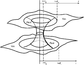
Figure 1: A $t=\mbox{constant}$ embedding diagram for the wormhole geometry. There is a throat at $r=r_{0}$ and stellar boundaries at $r=d_{\pm}$ where the system must smoothly join the vacuum.

In the curvature coordinates, labeled in figure 1, one usually employs the following line element:

$$ds^{2}=-e^{\gamma(r,t)_{\pm}}\,dt^{2}+e^{\alpha(r,t)_{\pm}}\,dr^{2}+r^{2}\,d\theta^{2}+r^{2}\sin^{2}(\theta)\,d\phi^{2}+a(t)\,d\Omega^{2}_{(D-4)},$$ (1)

where we have included the possibility of extra dimensions via $d\Omega^{2}_{(D-4)}$ thus yielding a warped product manifold of $M^{4}\times S^{D-4}$. The line element on a unit $D-4$ sphere is:

$$d\Omega^{2}_{(D-4)}=\left[d\psi_{(0)}^{2}+\sum_{n=1}^{D-5}d\psi_{(n)}^{2}\left(\prod_{m=1}^{n}\sin^{2}\psi_{(m-1)}\right)\right].$$

This chart, though useful, is not ideal for analysis of the throat. First, there is a coordinate singularity at $r=r_{0}$. Also, an explicit junction occurs here in these coordinates which must be addressed via the introduction of an “upper” chart and a “lower” chart (the $+$ and $-$ indicated above). Therefore, one must carefully consider junction conditions at the throat to possess an acceptable patching from the upper to lower chart.

Alternately, another common chart is the proper radius chart whose line element is given by:

$$ds^{2}=-e^{\mu(l,t)_{\pm}}\,dt^{2}+dl^{2}+r(l)^{2}\,d\theta^{2}+r(l)^{2}\sin^{2}(\theta)\,d\phi^{2}+a(t)\,d\Omega^{2}_{(D-4)},$$ (2)

where $l(r)$ is the (signed) proper radial coordinate:

$$l(r)=\pm\int_{r_{0}}^{r}e^{\alpha(r^{\prime})/2}dr^{\prime}.$$ (3)

Here the lower sheet in figure 1 corresponds to the $-$ sign in (3) and the upper sheet corresponds to the $+$, the throat located at $l=0$. Although continuous, the profile curve is not manifest in this chart. It is desirable in wormhole physics to retain the profile curve in calculations since one can prescribe properties of the wormhole via manipulation of the profile curve.

We choose to employ another, “global”, chart which we briefly introduced in [35]. The relation between this chart and the curvature coordinates of (1) is illustrated in figure 2.

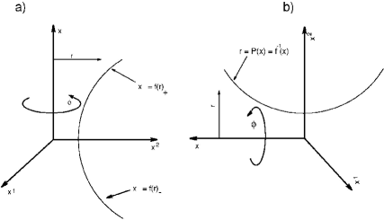
Figure 2: a) A cross section near the throat of a wormhole embedding function for $t=\mbox{constant}$. The function $x=f_{\pm}(r)$ represents the profile curve in the curvature coordinates. b) By rotating this curve, we invert the function $f(r)$ thus generating the profile curve $r=f^{-1}(x)=:P(x)$ in a coordinate system which is continuous across the throat.

To generate this coordinate system, one starts with the standard curvature coordinates. These consist of the upper and lower charts with profile curves given by $f(r)_{+}$ for $x>0$ and $f(r)_{-}$ for $x<0$ (refer to figure 2a). Rotating the $x\mbox{-}x^{2}$-plane about the $x^{1}$-axis of figure 2a by $\pi/2$, we can study the profile curve as parameterized by the coordinate $x$. That is, the profile curve given by $r=P(x)$ (see figure 2b). The coordinate $x$ belongs to an interval containing $x=0$, the throat of the wormhole. In this parameterization, the function $P(x)$ is assumed to be continuous at $x=0$ since an acceptable wormhole requires $\lim_{x\rightarrow 0^{+}}P(x)=\lim_{x\rightarrow 0^{-}}P(x)=P(0)$. Of course, the function $P(x)$ is not completely arbitrary and must possess the correct properties to describe a wormhole. These will be discussed below. (Also, the profile function $P(x)$ must be at least of class $C^{4}$ to generate an acceptable metric.) We concentrate in this paper on the region $x\geq 0$ as the physical results are the same for $x<0$ and calculations can easily be modified to include $x<0$.

The surface of revolution generated by rotating the curve in figure 2b about the $x$-axis (the direction of $\phi$) possesses the induced metric:

$$d\sigma^{2}=\left[1+P(x)_{,x}^{2}\right]\,(dx)^{2}+P(x)^{2}\,(d\phi)^{2}.$$ (4)

2.1 The general case

Any time dependent wormhole must possess a metric of the form (4) on the $x\mbox{-}\phi$-sub-manifold. Therefore, the corresponding spacetime metric may be written as

$$ds^{2} = -e^{\gamma(x,t)}\,dt^{2}+e^{\lambda(x,t)}\left\{\left[1+P(x)_{,x}^{2}\right]\,dx^{2}+P(x)^{2}\,d\theta^{2}+P(x)^{2}\sin^{2}\theta\,d\phi^{2}\right\}$$ (5)

$$+a(t)\,d\Omega_{(D-4)}^{2}\;.$$

Notice that for constant $t$, (5) possesses the desired hypersurface metric as well as those conformally related to it. At the wormhole throat, we must have $P(x)_{,x}=0$ and this condition is easily satisfied in this coordinate system with well behaved metric. (Note that in the standard curvature coordinates, the throat condition $f(r)_{,r}\rightarrow\infty$ yields a singular metric!) We denote the stellar boundary in the new chart as $x=x_{b\pm}$ where the $\pm$ indicate the left and right boundaries respectively. Note that $x_{b+}$ does not necessarily have to equal $-x_{b-}\;\;$.

The Einstein field equations,

$$R^{\mu}_{\;\nu}-\frac{1}{2}R\,\delta^{\mu}_{\;\nu}+\Lambda\,\delta^{\mu}_{\;\nu}=8\pi T^{\mu}_{\;\nu},$$ (6)

govern the geometry. These equations along with ansatz (5) yield the following differential equations:

$$-\frac{1}{4}\left\{e^{-\gamma(x,t)}\left[\frac{1}{2}(D-5)(D-4)\left(\frac{a(t)_{,t}}{a(t)}\right)^{2}+3(D-4)\lambda(x,t)_{,t}\frac{a(t)_{,t}}{a(t)}+3\lambda(x,t)_{,t}^{2}\right]\right.$$

$$+\frac{2(D-5)(D-4)}{a(t)}+e^{-\lambda(x,t)}\left[1+P(x)^{2}_{,x}\right]^{-1}\left[\frac{4}{P(x)^{2}}-\lambda(x,t)_{,x}^{2}-4\lambda(x,t)_{,x,x}\right.$$

$$\left.-\frac{8}{P(x)}\lambda(x,t)_{,x}P(x)_{,x}\right]\left.+4e^{-\lambda(x,t)}\left[1+P(x)^{2}_{,x}\right]^{-2}P(x)_{,x,x}\left[P(x)_{,x}\lambda(x,t)_{,x}-\frac{2}{P(x)}\right]\right\}$$

$$=8\pi T^{t}_{\;t}-\Lambda,$$ (7)

$$-\frac{1}{4}\left\{e^{-\gamma(x,t)}\left[\frac{1}{2}(D-7)(D-4)\left(\frac{a(t)_{,t}}{a(t)}\right)^{2}+2(D-4)\lambda(x,t)_{,t}\frac{a(t)_{,t}}{a(t)}+3\lambda(x,t)_{,t}^{2}\right.\right.$$

$$\left.-2\gamma(x,t)_{,t}\lambda(x,t)_{,t}+2(D-4)\frac{a(t)_{,t,t}}{a(t)}+4\lambda(x,t)_{,t,t}-(D-4)\gamma(x,t)_{,t}\frac{a(t)_{,t}}{a(t)}\right]$$

$$+\frac{2(D-5)(D-4)}{a(t)}+e^{-\lambda(x,t)}\left[1+P(x)^{2}_{,x}\right]^{-1}\left[\frac{4}{P(x)^{2}}-2\lambda(x,t)_{,x}\gamma(x,t)_{,x}-\lambda(x,t)_{,x}^{2}\right.$$

$$-\left.\left.\frac{4}{P(x)}P(x)_{,x}\left(\gamma(x,t)_{,x}+\lambda(x,t)_{,x}\right)\right]\right\}=8\pi T^{x}_{\;x}-\Lambda,$$ (8)

$$-\frac{1}{4}e^{-\gamma(x,t)}\left[2\gamma(x,t)_{,x}\lambda(x,t)_{,t}-4\lambda(x,t)_{,x,t}+(D-4)\gamma(x,t)_{,x}\frac{a(t)_{,t}}{a(t)}\right]=8\pi T^{t}_{\;x},$$ (9)

$$-\frac{1}{4}\left\{e^{-\gamma(x,t)}\left[\frac{1}{2}(D-7)(D-4)\left(\frac{a(t)_{,t}}{a(t)}\right)^{2}+2(D-4)\lambda(x,t)_{,t}\frac{a(t)_{,t}}{a(t)}+3\lambda(x,t)_{,t}^{2}\right.\right.$$

$$\left.+4\lambda(x,t)_{,t,t}+2(D-4)\frac{a(t)_{,t,t}}{a(t)}-2\lambda(x,t)_{,t}\gamma(x,t)_{,t}-(D-4)\gamma(x,t)_{,t}\frac{a(t)_{,t}}{a(t)}\right]$$

$$+\frac{2(D-5)(D-4)}{a(t)}-2e^{-\lambda(x,t)}\left[1+P(x)^{2}_{,x}\right]^{-1}\left[\lambda(x,t)_{,x,x}+\gamma(x,t)_{,x,x}\right.$$

$$+\lambda(x,t)_{,x}\frac{P(x)_{,x}}{P(x)}+\left.\frac{1}{2}\gamma(x,t)_{,x}^{2}+\frac{P(x)_{,x}}{P(x)}\gamma(x,t)_{,x}\right]$$

$$+\left.2P(x)_{,x,x}e^{-\lambda(x,t)}\left[1+P(x)^{2}_{,x}\right]^{-2}\left[P(x)_{,x}\left(\lambda(x,t)_{,x}+\gamma(x,t)_{,x}\right)-\frac{2}{P(x)}\right]\right\}$$

$$=8\pi T^{\theta}_{\;\theta}-\Lambda\equiv 8\pi T^{\phi}_{\;\phi}-\Lambda\;,$$ (10)

$$\frac{1}{4}\left\{e^{-\gamma(x,t)}\left[-\frac{1}{2}(D-8)(D-5)\left(\frac{a(t)_{,t}}{a(t)}\right)^{2}+(D-5)\frac{a(t)_{,t}}{a(t)}\left(\gamma(x,t)_{,t}-3\lambda(x,t)_{,t}\right)\right.\right.$$

$$\left.-6\lambda(x,t)_{,t}^{2}+3\gamma(x,t)_{,t}\lambda(x,t)_{,t}-6\lambda(x,t)_{,t,t}-2(D-5)\frac{a(t)_{,t,t}}{a(t)}\right]-\frac{2(D-5)(D-6)}{a(t)}$$

$$+2e^{-\lambda(x,t)}\left[1+P(x)_{,x}^{2}\right]^{-1}\left[4\lambda(x,t)_{,x}\frac{P(x)_{,x}}{P(x)}-\frac{2}{P(x)^{2}}+\frac{1}{2}\left(\lambda(x,t)_{,x}^{2}+\gamma(x,t)_{,x}^{2}\right)\right.$$

$$\left.+2\lambda(x,t)_{,x,x}+\gamma(x,t)_{,x,x}+\frac{2}{P(x)}\gamma(x,t)_{,x}P(x)_{,x}+\frac{1}{2}\gamma(x,t)_{,x}\lambda(x,t)_{,x}\right]$$

$$\left.+2e^{-\lambda(x,t)}\left[1+P(x)^{2}_{,x}\right]^{-2}\left[\frac{4}{P(x)}P(x)_{,x,x}-P(x)_{,x}P(x)_{,x,x}\left(\gamma(x,t)_{,x}+2\lambda(x,t)_{,x}\right)\right]\right\}$$

$$=8\pi T^{A}_{\;A}-\Lambda.$$ (11)

(Here the index $A$ is not summed!)

The conservation laws,

$$T^{\mu}_{\;\nu;\mu}=0,$$

yield two non-trivial equations:

$$T^{\mu}_{\;t;\mu} = \frac{1}{2}\left\{(D-4)\frac{a(t)_{,t}}{a(t)}\left[T^{t}_{\;t}-T^{A}_{\;A}\right]-\lambda(x,t)_{,t}\left[T^{x}_{\;x}+2T^{\theta}_{\;\theta}\right]\right.$$ (12)

$$+\frac{4}{P(x)}P(x)_{,x}T^{x}_{\;t}+3\lambda(x,t)_{,t}T^{t}_{\;t}+3\lambda(x,t)_{,x}T^{x}_{\;t}+2\left[T^{x}_{\;t,x}+T^{t}_{\;t,t}\right]$$

$$+\left[1+P(x)_{,x}^{2}\right]^{-1}\left[2P(x)_{,x}P(x)_{,x,x}T^{x}_{\;t}-\gamma(x,t)_{,x}e^{\gamma(x,t)-\lambda(x,t)}T^{t}_{\;x}\right]\left.\right\}=0$$

and

$$T^{\mu}_{\;x;\mu} = \frac{1}{2}\left\{2T^{t}_{\;x,t}+2T^{x}_{\;x,x}-\lambda(x,t)_{,t}e^{\lambda(x,t)-\gamma(x,t)}\left[1+P(x)_{,x}^{2}\right]T^{x}_{\;t}\right.$$ (13)

$$-\gamma(x,t)_{,x}T^{t}_{\;t}+T^{t}_{\;x}\left[\gamma(x,t)_{,t}+2\lambda(x,t)_{,t}+(D-4)\frac{a(t)_{,t}}{a(t)}\right]$$

$$+T^{x}_{\;x}\left[\gamma(x,t)_{,x}+2\lambda(x,t)_{,x}+\frac{4}{P(x)}P(x)_{,x}\right]-2T^{\theta}_{\;\theta}\left[\lambda(x,t)_{,x}+\frac{2}{P(x)}P(x)_{,x}\right]\left.\right\}$$

$$= 0.$$

To study the singularity structure of the manifold, the orthonormal Riemann components will be needed. These, as well as those related by symmetry, are furnished by the following:

$$R_{\hat{t}\hat{x}\hat{t}\hat{x}} = -\frac{1}{4}\left\{e^{-\gamma(x,t)}\left[2\lambda(x,t)_{,t,t}+\lambda(x,t)_{,t}^{2}-\lambda(x,t)_{,t}\gamma(x,t)_{,t}\right]\right.$$ (14)

$$+e^{-\lambda(x,t)}\left[1+P(x)^{2}_{,x}\right]^{-1}\left[\lambda(x,t)_{,x}\gamma(x,t)_{,x}-\gamma(x,t)_{,x}^{2}-2\gamma(x,t)_{,x,x}\right]$$

$$\left.+2e^{-\lambda(x,t)}\left[1+P(x)^{2}_{,x}\right]^{-2}\gamma(x,t)_{,x}P(x)_{,x}P(x)_{,x,x}\right\},$$

$$R_{\hat{t}\hat{\theta}\hat{t}\hat{\theta}} = -\frac{1}{4}\left\{e^{-\gamma(x,t)}\left[2\lambda(x,t)_{,t,t}+\lambda(x,t)_{,t}^{2}-\gamma(x,t)_{,t}\lambda(x,t)_{,t}\right]\right.$$ (15)

$$+\left.e^{-\lambda(x,t)}\left[1+P(x)_{,x}^{2}\right]^{-1}\left[\lambda(x,t)_{,x}\gamma(x,t)_{,x}-2\gamma(x,t)_{,x}\frac{P(x)_{,x}}{P(x)}\right]\right\},$$

$$R_{\hat{t}\hat{\theta}\hat{x}\hat{\theta}} = \frac{1}{2}e^{-\left[\gamma(x,t)+\lambda(x,t)\right]/2}\left[1+P(x)^{2}_{,x}\right]^{-1/2}\left[\frac{1}{2}\lambda(x,t)_{,t}\gamma(x,t)_{,x}-\lambda(x,t)_{,x,t}\right],$$ (16)

$$R_{\hat{x}\hat{\theta}\hat{x}\hat{\theta}} = -\frac{1}{4P(x)}\left\{2e^{-\lambda(x,t)}\left[1+P(x)^{2}_{,x}\right]^{-2}\left[2P(x)_{,x,x}-P(x)P(x)_{,x}P(x)_{,x,x}\lambda(x,t)_{,x}\right]\right.$$ (17)

$$\left.+2e^{-\lambda(x,t)}\left[1+P(x)^{2}_{,x}\right]^{-1}\left[\lambda(x,t)_{,x}P(x)_{,x}+\lambda(x,t)_{,x,x}P(x)\right]\right.$$

$$\left.-e^{-\gamma(x,t)}\lambda(x,t)_{,t}^{2}P(x)\right\},$$

$$R_{\hat{\theta}\hat{\phi}\hat{\theta}\hat{\phi}} = \frac{1}{4P(x)^{2}}\left\{e^{-\lambda(x,t)}\left[1+P(x)^{2}_{,x}\right]^{-1}\left[4-\lambda(x,t)_{,x}^{2}P(x)^{2}-4\lambda(x,t)_{,x}P(x)_{,x}P(x)\right]\right.$$ (18)

$$\left.+e^{-\gamma(x,t)}\lambda(x,t)_{t}^{2}P(x)^{2}\right\},$$

$$R_{\hat{t}\hat{A}\hat{t}\hat{A}} = \frac{e^{-\gamma(x,t)}}{4a(t)^{2}}\left[\gamma(x,t)_{,t}a(t)_{,t}a(t)-2a(t)_{,t,t}a(t)+a(t)_{,t}^{2}\right],$$ (19)

$$R_{\hat{t}\hat{A}\hat{x}\hat{A}} = \frac{1}{4a(t)}e^{-\left[\gamma(x,t)+\lambda(x,t)\right]/2}\left[1+P(x)^{2}_{,x}\right]^{-1/2}\gamma(x,t)_{,x}a(t)_{,t},$$ (20)

$$R_{\hat{x}\hat{A}\hat{x}\hat{A}} = \frac{1}{4}e^{-\gamma(x,t)}\lambda(x,t)_{,t}\frac{a(t)_{,t}}{a(t)},$$ (21)

$$R_{\hat{\theta}\hat{A}\hat{\theta}\hat{A}} = \frac{1}{4}e^{-\gamma(x,t)}\lambda(x,t)_{,t}\frac{a(t)_{,t}}{a(t)},$$ (22)

$$R_{\hat{A}\hat{B}\hat{A}\hat{B}}= \frac{1}{4}\left[\frac{4}{a(t)}+\left(\frac{a(t)_{,t}}{a(t)}\right)^{2}e^{-\gamma(x,t)}\right].$$ (23)

Here hatted indices indicate quantities calculated in the orthonormal frame. It is interesting to note that the Riemann components are independent of the number of compact dimensions. A singular manifold results if any of the following conditions occur: $a(t)=0$, $a(t)_{,t}\rightarrow\pm\infty$, $a(t)_{,t,t}\rightarrow\pm\infty$, $\gamma(x,t)\rightarrow-\infty$, $\gamma(x,t)_{,t}\rightarrow\pm\infty$, $\gamma(x,t)_{,x}\rightarrow\pm\infty$, $\gamma(x,t)_{,x,x}\rightarrow\pm\infty$, $\lambda(x,t)\rightarrow-\infty$, , $\lambda(x,t)_{,t}\rightarrow\pm\infty$, , $\lambda(x,t)_{,x}\rightarrow\pm\infty$, $\lambda(x,t)_{,t,t}\rightarrow\pm\infty$, $\lambda(x,t)_{,x,x}\rightarrow\pm\infty$ and $\lambda(x,t)_{,x,t}\rightarrow\pm\infty$.

Since the profile curve has not been specified, the above system of equations may be used to model almost any spherically symmetric spacetime with arbitrary number of compact dimension. We wish here to study a wormhole system and therefore must, at the very least, impose the condition that $x=0$ is a local minimum of the profile curve. The sufficient conditions for such a minimum are the following:

• $P(x)_{,x|_{x=0}}$ must vanish.

• $P(x)_{,x}$, must change sign at the throat. $P(x)_{,x}>0$ for $x>0$ and $P(x)_{,x}<0$ for $x<0$ (at least near the throat).

• $P(x)$ must possess a positive second derivative at least near the throat region.

Since there will be a cut-off at $x=x_{b\pm}$, where the solution is joined to vacuum, no specification needs to be made for $x>x_{b+}$ and $x<x_{b-}$.

With little loss of generality, we may model any near throat geometry with the profile function

$$P(x)= P_{0}+A^{2}x^{2n}\exp\left[h^{2}(x)\right],$$ (24a)

$$P(x)_{,x}= 2A^{2}x^{2n}\exp\left[h^{2}(x)\right]\left[\frac{n}{x}+h(x)h(x)_{,x}\right],$$ (24b)

$$P(x)_{,x,x}= 2A^{2}x^{2n}\exp\left[h^{2}(x)\right]\left\{2\left[\frac{n}{x}+h(x)\,h(x)_{,x}\right]^{2}\right.$$

$$-\left.\frac{n}{x^{2}}+h(x)\,h(x)_{,x,x}+h(x)_{,x}^{2}\right\}.$$ (24c)

Here $n=1,\,2,\,3,\,4,\ldots$, and $P_{0}>0$ is the radius of the throat. The quantity $A$ is any non-zero constant and $h(x)$ a sufficiently differentiable (at least $C^{4}$) arbitrary function. The positive constant $n$ is restricted to integers for convenience. One may also model wormholes for non-integer $n$ however, reasonable physics places restrictions on the acceptable values of $n$ as will be shown later. Such a function (24a) for $P(x)$ is capable of describing infinitely many spherically symmetric wormholes at least near the vicinity of the throat.

As mentioned in the introduction, an interesting property of static wormholes is that such systems must violate the WEC even if only in some arbitrarily small region. Time dependent analogues in four dimensions have been examined in the context of inflationary scenarios [40], [49] as well as general local geometry at the near throat region [43]. However, here we wish to study compact objects joined to an acceptable vacuum with an arbitrary number of extra dimensions. Therefore, the properties of the stress-energy tensor are mainly determined by desirable physics and the junction conditions at the stellar boundary. It turns out that the presence of this boundary imposes some interesting restrictions on the wormhole structure.

2.2 The quasi-static case

The full field equations, given by (7 - 11) are too formidable to solve in generality with (24a) and reasonable stress-energy tensor. In four dimensional General Relativity, the static assumption is often made to keep the analysis tractable (for example, in many analytic studies of stellar structure [50] as well as wormholes [8]). This assumption is motivated by the observational fact that many stellar systems are slowly varying with time and therefore the time-dependence may be ignored. Here we make a similar assumption save for the fact that the radius of the extra dimensions may vary with time (for examples of theories where extra dimensions are explicitly static or time-dependent see [51], [52], [53], [54] and references therein.) Put another way, since the solutions to the differential equations are local, one may consider these solutions valid over a time interval where the gravitational field does not evolve appreciably in either the full space (the static case) or merely the non-compact space (the quasi-static case). Below we consider both situations. The latter case allows for the fact that, since the extra dimensions are not on an equal footing with the non-compact ones, they may evolve at a radically different rate than the non-compact dimensions. (In a warped product manifold such as (5), it is the vacuum which will determine the behaviour of the compactification radius, $a(t)$, if a vacuum-matter boundary is present. It turns out that even if a vacuum appears static in the non-compact $M^{4}$, it will support a compactification radius which can vary rapidly with time as will be seen in section 3.1.1.)

The above cases are of particular interest since static four dimensional wormholes have now been well studied and many of their properties determined. However, in light of the possibility of higher dimensions, it is useful to extend studies to the higher dimensional counter-parts of these cases. It turns out that the higher dimensional static and “quasi-static” wormholes may differ considerably from the four dimensional ones. Some results in this study are also valid for trivial topology and therefore will shed some light on the behaviour of “regular” static stars when one allows for the time dependent and time independent extra dimensions.

The quasi-static configuration possesses line element:

$$ds^{2}=-e^{\gamma(x)}\,dt^{2}+\left[1+P(x)^{2}_{,x}\right]\,dx^{2}+P(x)^{2}\,d\theta^{2}+P(x)^{2}\sin^{2}\theta\,d\phi^{2}+a(t)\,d\Omega_{(D-4)}^{2}\;.$$ (25)

and yield the corresponding Einstein equations:

$$-\frac{1}{4}\left\{\frac{1}{2}e^{-\gamma(x)}(D-5)(D-4)\left(\frac{a(t)_{,t}}{a(t)}\right)^{2}+\frac{2(D-5)(D-4)}{a(t)}+\left[1+P(x)_{,x}^{2}\right]^{-1}\frac{4}{P(x)^{2}}\right.$$

$$\left.-8\left[1+P(x)_{,x}^{2}\right]^{-2}\frac{P(x)_{,x,x}}{P(x)}\right\}=8\pi T^{t}_{\;t}-\Lambda,$$ (26a)

$$-\frac{1}{4}\left\{e^{-\gamma(x)}\left[\frac{1}{2}(D-7)(D-4)\left(\frac{a(t)_{,t}}{a(t)}\right)^{2}+2(D-4)\frac{a(t)_{,t,t}}{a(t)}\right]+\frac{2(D-5)(D-4)}{a(t)}\right.$$

$$+4\left[1+P(x)_{,x}^{2}\right]^{-1}\left[\frac{1}{P(x)^{2}}-\gamma(x)_{,x}\frac{P(x)_{,x}}{P(x)}\right]\left.\right\}=8\pi T^{x}_{\;x}-\Lambda,$$ (26b)

$$-\frac{(D-4)}{4}e^{-\gamma(x)}\gamma_{,x}\frac{a(t)_{,t}}{a(t)}=8\pi T^{t}_{\;x}$$ (26c)

$$-\frac{1}{4}\left\{e^{-\gamma(x)}\left[\frac{1}{2}(D-7)(D-4)\left(\frac{a(t)_{,t}}{a(t)}\right)^{2}+2(D-4)\frac{a(t)_{,t,t}}{a(t)}\right]+\frac{2(D-5)(D-4)}{a(t)}\right.$$

$$-2\left[1+P(x)_{,x}^{2}\right]^{-1}\left[\gamma(x)_{,x,x}+\frac{1}{2}\gamma(x)^{2}_{,x}+\frac{P(x)_{,x}}{P(x)}\gamma(x)_{,x}\right]$$

$$+2P(x)_{,x,x}\left[1+P(x)_{,x}^{2}\right]^{-2}\left[P(x)_{,x}\gamma(x)_{,x}-\frac{2}{P(x)}\right]\left.\right\}=8\pi T^{\theta}_{\;\theta}-\Lambda\equiv 8\pi T^{\phi}_{\;\phi}-\Lambda,$$ (26d)

$$-\frac{1}{4}\left\{e^{-\gamma(x)}\left[\frac{1}{2}(D-8)(D-5)\left(\frac{a(t)_{,t}}{a(t)}\right)^{2}+2(D-5)\frac{a(t)_{,t,t}}{a(t)}\right]+\frac{2(D-5)(D-6)}{a(t)}\right.$$

$$+2\left[1+P(x)_{,x}^{2}\right]^{-1}\left[\frac{2}{P(x)^{2}}-\frac{1}{2}\gamma(x)^{2}_{,x}-\gamma(x)_{,x,x}-2\gamma(x)_{,x}\frac{P(x)_{,x}}{P(x)}\right]$$

$$+2\left[1+P(x)_{,x}^{2}\right]^{-2}\left[\gamma(x)_{,x}P(x)_{,x}P(x)_{,x,x}-4\frac{P(x)_{,x,x}}{P(x)}\right]\left.\right\}=8\pi T^{A}_{\;A}-\Lambda\>.$$ (26e)

The conservation laws simplify to:

$$T^{\mu}_{\;t;\mu}= \frac{1}{2}\left\{(D-4)\frac{a(t)_{,t}}{a(t)}\left[T^{t}_{\;t}-T^{A}_{\;A}\right]+4\frac{P(x)_{,x}}{P(x)}T^{x}_{\;t}+2\left[T^{x}_{\;t,x}+T^{t}_{\;t,t}\right]\right.$$

$$\left.+\left[1+P(x)_{,x}^{2}\right]^{-1}\left[2P(x)_{,x}P(x)_{,x,x}T^{x}_{\;t}-\gamma(x)_{,x}e^{\gamma(x)}T^{t}_{\;x}\right]\right\}=0,$$ (27a)

$$T^{\mu}_{\;x,\mu}= \frac{1}{2}\left\{2T^{t}_{\;x,t}+2T^{x}_{\;x,x}-\gamma(x)_{,x}T^{t}_{\;t}+(D-4)\frac{a(t)_{,t}}{a(t)}T^{t}_{\;x}\right.$$

$$\left.+\left[\gamma(x)_{,x}+4\frac{P(x)_{,x}}{P(x)}\right]T^{x}_{\;x}-4T^{\theta}_{\;\theta}\frac{P(x)_{,x}}{P(x)}\right\}=0,$$ (27b)

and the orthonormal Riemann components are furnished by:

$$R_{\hat{t}\hat{x}\hat{t}\hat{x}}= \frac{1}{4}\left\{\left[1+P(x)_{,x}^{2}\right]^{-1}\left[\gamma(x)^{2}_{,x}+2\gamma(x)_{,x,x}\right]\right.$$

$$\left.+2\left[1+P(x)_{,x}^{2}\right]^{-2}\gamma(x)_{,x}P(x)_{,x}P(x)_{,x,x}\right\}$$ (28a)

$$R_{\hat{t}\hat{\theta}\hat{t}\hat{\theta}}= \frac{1}{2}\left[1+P(x)_{,x}^{2}\right]^{-1}\gamma(x)_{,x}\frac{P(x)_{,x}}{P(x)}$$ (28b)

$$R_{\hat{x}\hat{\theta}\hat{x}\hat{\theta}}= -\left[1+P(x)_{,x}^{2}\right]^{-2}\frac{P(x)_{,x,x}}{P(x)^{2}}$$ (28c)

$$R_{\hat{\theta}\hat{\phi}\hat{\theta}\hat{\phi}}= \frac{1}{P(x)^{2}}\left[1+P(x)_{,x}^{2}\right]^{-1}$$ (28d)

$$R_{\hat{t}\hat{A}\hat{t}\hat{A}}= \frac{e^{-\gamma(x)}}{4a(t)^{2}}\left[a(t)^{2}_{,t}-2a(t)a(t)_{,t,t}\right]$$ (28e)

$$R_{\hat{t}\hat{A}\hat{x}\hat{A}}= \frac{1}{4a(t)^{2}}e^{-\gamma(x)/2}\left[1+P(x)_{,x}^{2}\right]^{-1/2}\gamma(x)_{,x}a(t)_{,t}$$ (28f)

$$R_{\hat{A}\hat{B}\hat{A}\hat{B}}= \frac{1}{4}\left[\frac{4}{a(t)}+\left(\frac{a(t)_{,t}}{a(t)}\right)^{2}e^{-\gamma(x)}\right].$$ (28g)

By analyzing the orthonormal Riemann components (28a- 28d) corresponding to the four non-compact dimensions, it can be seen that this indeed describes a system which is static in the first four dimensions. From equations (28e-28g) it is clear that time dependence of the gravitational field is experienced only by parallel transport of vectors around closed loops which venture into the higher dimensions. Therefore, an observer unaware of the presence of the extra dimensions will “see” only a static wormhole or star.

3 Physical structure

3.1 The vacuum

Isolated systems such as those described here should possess some boundary differentiating the vacuum from the matter which supports the wormhole. In four dimensions there is the Birkhoff’s theorem which dictates that the only acceptable spherically symmetric vacuum is locally equivalent to the Schwarzschild (or Schwarschild-(anti) deSitter for non-zero cosmological constant) vacuum [55]. It turns out that a similar theorem holds for any higher number of non-compact dimensions [56], [57], [27].

By studying the vacuum version of equations (26a)-(26e) we encounter the possibility for several vacua which fall into two general classes. From equation (26c) we see that for $D>4$, $G^{t}_{\;x}=0$ implies that either $\gamma\equiv\gamma_{0}$ or that $a(t)\equiv\varepsilon$, where $\gamma_{0}$ and $\varepsilon$ are constants. For both cases, we begin by solving the linear combination

$$G^{t}_{\;t}-G^{x}_{\;x}=0\;.$$ (29)

3.1.1 The vacuum $\gamma\equiv\gamma_{0}$

In this situation the equation (29) provides the following set of equations

$$\left[\frac{a(t)_{,t}}{a(t)}\right]^{2}-2\frac{a(t)_{,t,t}}{a(t)}=k\frac{e^{\gamma_{0}}}{D-4}=:k_{0},$$ (30a)

$$8\frac{P(x)_{,x,x}}{P(x)}\left[1+P(x)_{,x}^{2}\right]^{-2}=k.$$ (30b)

At the moment, the separation constant, $k$, may be positive, zero, or negative corresponding respectively to elliptic, parabolic and hyperbolic behaviour of the compact dimensions.

It is found that one cannot satisfy all vacuum field equations for the cases $k>0$ and $k=0$ and therefore we concentrate only on the $k<0$ scenario. The solutions of (30a) and (30b) for $k<0$ are:

$$a(t)=\left[a_{0}e^{\omega t}+b_{0}e^{-\omega t}\right]^{2}$$ (31)

and

$$P(x)=\left[\frac{8}{|k|}-\left(x-x_{0}\right)^{2}\right]^{1/2},$$ (32)

with $\omega:=\sqrt{\frac{|k|e^{\gamma_{0}}}{4(D-4)}}$ and $a_{0}$ and $b_{0}$ constants of integration. After long calculations, all vacuum equations may be solved provided that:

$$|k|=\frac{8}{D-2}\,\Lambda>0\;\;\;\;\mbox{and}\;\;\;\;a_{0}b_{0}=\frac{D-4}{|k|}>0$$

indicating a deSitter $R$-type vacuum with $\frac{D-2}{\Lambda}>(x-x_{0})^{2}\geq 0$. The constant $x_{0}$ corresponds to the “centre” of the deSitter shell. The surface $(x-x_{0})^{2}=\frac{D-2}{\Lambda}$ is not an event horizon since, in the coordinate system of (5) the presence an event horizon is indicated by the condition $g_{tt}=0$. The vacuum metric, (25), is therefore given by

$$ds^{2}_{vac_{1}} = -e^{\gamma_{0}}\,dt^{2}+\left[1+\frac{(x-x_{0})^{2}}{\frac{D-2}{\Lambda}-(x-x_{0})^{2}}\right]\,dx^{2}+\left[\frac{D-2}{\Lambda}-(x-x_{0})^{2}\right]\,d\Omega_{(2)}^{2}$$ (33)

$$+\left[a_{0}e^{\omega t}+\frac{(D-4)(D-2)}{8\Lambda\,a_{0}}e^{-\omega t}\right]^{2}\,d\Omega_{(D-4)}^{2}.$$

This vacuum differs from the vacua considered below and therefore there is no unique vacuum when one allows for the possibility of compact extra dimensions.

If this is to be considered the global vacuum, then the wormhole system must actually describe a “dumbbell” wormhole [13], [58]. Although topologically trivial, such systems are considered wormholes in the literature [43]. This scenario is shown qualitatively in figure 3a. Alternately, one can patch one or both spatially-closed universes to an open (non-vacuum) universe thus creating the systems shown in figure 3b and 3c.

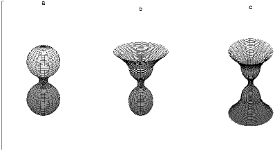
Figure 3: Rotated profile curves representing: a) A dumbbell universe consisting of two spatially-closed universes connected by a narrow throat, b) A spatially-closed universe connected to an open universe, c) Two open universes connected by a wormhole.

3.1.2 The vacuum $a=\varepsilon$

For this case, the equation (29) provides a useful relation between $\gamma(x)_{,x}$ and the derivatives of $P(x)$:

$$\gamma(x)_{,x}=2\frac{P(x)_{,x,x}}{P(x)_{,x}\left[1+P(x)_{,x}^{2}\right]}\;.$$ (34)

This may be used in the equation $G^{\theta}_{\;\theta}-G^{A}_{\;A}=0$ yielding a differential equation for $P(x)$ only. The resulting autonomous equation may be solved implicitly for $P(x)$:

$$\pm\int\left[\frac{\frac{D-5}{3\varepsilon}P^{3}-E_{0}}{-\frac{D-5}{3\varepsilon}P^{3}+P+E_{0}}\right]^{1/2}dP=x-x_{0}\;,$$ (35)

with $E_{0}$ a constant resulting from integration. We consider first the $D=5$ geometry.

For the case $D=5$ one must demand that $E_{0}<0$ and (35) may be readily integrated. The profile curve for this case is

$$P(x)_{D=5}=\left[|E_{0}|+\frac{(x-x_{0})^{2}}{4|E_{0}|}\right],$$ (36)

which, with (34) gives the spatially-open vacuum with zero cosmological constant:

$$ds^{2}_{5D\;vac} = -\frac{(x-x_{0})^{2}}{4|E_{0}|^{2}+(x-x_{0})^{2}}\,dt^{2}+\left[1+\frac{(x-x_{0})^{2}}{4|E_{0}|^{2}}\right]\,dx^{2}$$ (37)

$$+\left[|E_{0}|+\frac{(x-x_{0})^{2}}{4|E_{0}|}\right]^{2}\,d\Omega_{(2)}^{2}+\varepsilon\,d\psi_{(0)}^{2}.$$

This is essentially the Schwarzschild solution crossed with one compact dimension and $|E_{0}|$ is related to the gravitating mass, $M$, via $|E_{0}|:=2M$. The event horizon exists at $x=x_{0}$.

For the case $E_{0}=0$ and $D>5$ the equation (35) may also be explicitly solved for $P(x)$ as

$$P(x)=\left[\frac{3\varepsilon}{D-5}-\left(x-x_{0}\right)^{2}\right]^{1/2}.$$ (38)

This, along with equation (34) yields the metric function:

$$e^{\gamma(x)}=\kappa_{0}^{2}\left(x-x_{0}\right)^{2},\;\;\;\;\;\;\kappa_{0}\mbox{ a constant}$$ (39)

and therefore the vacuum line element, (25), is given by

$$ds^{2}_{D>5\;vac} = -\kappa_{0}^{2}\left(x-x_{0}\right)^{2}\,dt^{2}+\left[1+\frac{(x-x_{0})^{2}}{\frac{3\varepsilon}{D-5}-(x-x_{0})^{2}}\right]\,dx^{2}$$ (40)

$$+\left[\frac{3\varepsilon}{D-5}-(x-x_{0})^{2}\right]\,d\Omega^{2}_{(2)}+\varepsilon\,d\Omega^{2}_{(D-4)}.$$

This metric solves the vacuum field equations with cosmological constant:

$$\Lambda=\frac{(D-2)(D-5)}{2\varepsilon}\;.$$ (41)

The vacuum is spatially-closed with $\frac{3(D-2)}{2\Lambda}>(x-x_{0})^{2}\geq 0$. The surface $x=x_{0}$ is a cosmological horizon as is found in the deSitter universe and is of no concern if considering a traversable wormhole.

Although (35) cannot be explicitly integrated for the general case, it can be shown that the metrics described by this equation are similar to the four dimensional Kottler [59] solution with the value of the cosmological constant dictated by (41). The relation to the Kottler solution is not unexpected since, for constant $a(t)$, one has a direct product manifold. For $D=5$ the manifold structure is $M^{4}\times S^{1}$ with $S^{1}$ being intrinsically flat, thereby yielding zero cosmological constant as above. Similarly, for $D>5$, the compact dimensions yield an $S^{D-4}$ manifold, demanding positive cosmological constant.

An acceptable interval for (35) with $D>5$ and $E_{0}\neq 0$ is provided by the reality condition on (35). Note that this restriction again implies a spatially-closed universe.

3.2 Wormhole structure

In this section we discuss the matter region given by $x_{b}\geq x\geq 0$. We attempt to limit, or eliminate where possible, violations of the WEC as well as demonstrate how singularities and black-hole-event horizons may be avoided.

At the boundary, $x=x_{b}$, we employ the junction conditions of Synge [60] which read:

$$T^{\mu}_{\;\nu}\>\hat{n}^{\nu}_{\;\>|_{x=x_{b}}}=0,$$ (42)

where $\hat{n}^{\nu}$ is an outward pointing unit normal to the boundary. Explicitly, these conditions yield the following:

$$T^{t}_{\;x|_{x=x_{b}}}=0,$$ (43a)

$$T^{x}_{\;x|_{x=x_{b}}}=0.$$ (43b)

The junction condition (43a) dictates (referring to (26c)) that either $\gamma(x)_{,x}=0$ at the stellar boundary or that $a(t)\equiv\varepsilon$. We consider both cases. The first will be patched to the vacuum (33) and the latter to one of the static vacua.

We wish the stellar material to satisfy the weak energy condition (WEC) which is given by

$$T_{\mu\nu}V^{\mu}V^{\nu}\geq 0\;\;\;\;\forall\;\;\;\;\mbox{time-like}\;\;V^{\alpha}.$$ (44)

In the case of a non-diagonal stress-energy tensor, (44) yields the conditions:

$$T^{i}_{\;i}-T^{t}_{\;t}\geq 0\;\;\;\;\mbox{and}\;\;\;\;T^{t}_{\;t}\leq 0\,,\;\;\;\;i\neq x\>,\;\;\;\mbox{no summation},$$ (45)

along with one of the following:

$$\mbox{for }T^{x}_{\;x}\leq 0:\;\;\;T^{x}_{\;x}-T^{t}_{\;t}\geq 2\frac{e^{\gamma(x)/2}}{\left[1+P(x)_{,x}^{2}\right]^{1/2}}|T^{t}_{\;x}|,$$ (46a)

$$\mbox{for }T^{x}_{\;x}>0\mbox{ either }:$$

$$\frac{e^{\gamma(x)}}{\left[1+P(x)_{,x}^{2}\right]}(T^{t}_{\;x})^{2}+T^{x}_{\;x}T^{t}_{\;t}\leq 0$$ (46b)

or

$$0<\left[\frac{e^{\gamma(x)}}{\left[1+P(x)_{,x}^{2}\right]}\left(T^{t}_{\;x}\right)^{2}+T^{x}_{\;x}T^{t}_{\;t}\right]^{1/2}\leq\frac{e^{\gamma(x)/2}}{\left[1+P(x)_{,x}^{2}\right]^{1/2}}|T^{t}_{\;x}|-T^{x}_{\;x}.$$ (46c)

One could also write the above in the orthonormal frame which would eliminate the factors of the metric. However, for the analysis here it is more convenient to use the above form.

3.2.1 The $a\equiv\varepsilon$ wormhole

This case corresponds to a purely static wormhole. However, it will be shown that the presence of compact extra dimensions yield restrictions not present in the four dimensional static wormhole.

We attempt to satisfy the WEC (44) in the vicinity of the throat. If WEC violation occurs away from the throat, at $|x|=|x_{*}|$ say, one may attempt to place the stellar boundary at some $|x|<|x_{*}|$ to eliminate the WEC violation. An expansion near the throat utilizing (26a) and (24a yields:

$$-8\pi T^{t}_{\;t} \approx \frac{1}{P^{2}_{0}}-\frac{2}{D-2}\Lambda-\frac{4}{P_{0}}\left[2n^{2}-n\right]A^{2}e^{h^{2}(0)}x^{2n-2}$$ (47)

$$-\frac{8}{P_{0}}\left[2n^{2}+n\right]A^{2}e^{h^{2}(0)}h(0)h(x)_{,x\,|x=0}x^{2n-1}+\mathcal{O}(x^{2n}),$$

where the extra dimensions affect the matter energy density via the cosmological constant term (from equation 41). Here we see why reasonable physics restricts acceptable values of $n$ if one were to consider arbitrary real numbers for $n$. For $n<1$ a singular density (as well as $P(x)_{,x,x}$) results at the wormhole throat which yields a singular manifold. However, physical results in this paper are unchanged by dropping the integer restriction on $n$.

The best scenario from the point of view of energy conditions is that where $n>1$. This gives the largest possible energy density at the throat. Exactly at the throat ($x=0$) (47), with $n>1$, gives:

$$\left[-8\pi T^{t}_{\;t}\right]_{|x=0}=\frac{1}{P_{0}^{2}}-\frac{2}{D-2}\Lambda.$$ (48)

Demanding that (48) be non-negative (as required by WEC) and noting the relation between $\Lambda$ and $\varepsilon$ as dictated by (41) yields a particularly interesting result:

$$P_{0}^{2}<\frac{\varepsilon}{D-5}\;.$$ (49)

That is, if the energy density as seen by static observers is to be positive for $D>5$, the radius of the wormhole throat must be less than the radius of the extra dimensions. For $D=5$ and $n>1$, any radius is allowed. The greater the number of extra dimensions, the smaller a WEC respecting throat must be. If one considers $n=1$ then the radius must be even smaller than that dictated by (49) since the third term in (47) contributes. Note that the above restrictions are stronger than the purely geometric restriction in which the radius of the wormhole throat must be less than the radius of the closed universe (which in this case would read $P_{0}^{2}<3\varepsilon/(D-5)$.)

Next, we concentrate on the parallel pressure, $T^{x}_{\;x}$. This function will be derived in such a way as to satisfy as many physical requirements as possible (for example, no singularities). As well, junction condition (43b) must be met.

A necessary condition for the absence of singularities is that the derivative, $\gamma(x)_{,x}$, be finite. From the equation (26b) we find

$$\gamma(x)_{,x}=\frac{P(x)}{P(x)_{,x}}\left\{\left[1+P(x)_{,x}^{2}\right]\left[8\pi T^{x}_{\;x}-\frac{2}{D-2}\Lambda\right]+\frac{1}{P(x)^{2}}\right\},$$ (50)

where we have used the relation (41) to eliminate $\varepsilon$. For (50) to be finite at the throat, we must demand that the term in braces vanish at least as fast as $P(x)_{,x}$ near the throat. The behaviour of $P(x)_{,x}$ near the throat is of order $\mathcal{O}(x^{2n-1})$ and therefore we must demand that $8\pi T^{x}_{\;x}-\frac{2}{D-2}\Lambda\approx-\frac{1}{P_{0}^{2}}+\mathcal{O}(x^{2n-1})$. Also, $T^{x}_{\;x}$ must vanish at $x=x_{b}$. In terms of arbitrary functions, these condition may be enforced via

$$8\pi T^{x}_{\;x}-\frac{2}{D-2}\Lambda = -\frac{1}{P(x)^{2}}\cos\left[\left(\frac{x}{x_{b}+\alpha}\right)^{(2n)p}\frac{m\pi}{2}\right]\cosh\left[x^{s}\xi(x)\right]$$ (51)

$$+\kappa x^{q}\left(x-x_{b}\right)^{w}e^{\zeta(x)}.$$

Here, $\xi(x)$ and $\zeta(x)$ are arbitrary, differentiable functions. The constants are restricted as follows: $p\geq 1/2$, $m$ an odd integer, $s\geq n$, $q\geq 2n$, $w$ a positive integer and $\kappa$ a constant. The constant, $\alpha$, is set by the requirement that the right-hand-side of (51) is equal to $-2/(D-2)\;\Lambda$ when $x=x_{b}$. The second term on the right-hand-side of (51) is not required but is useful as a “fine tuning” function if we wish the solution to obey the WEC throughout most of the stellar bulk (if the first term is negative with too large a magnitude to respect the WEC, one may make this second term large and positive).

To study the WEC near the throat, $T^{x}_{\;x}$ is expanded in powers of $x$:

$$8\pi T^{x}_{\;x}\approx-\frac{1}{P_{0}^{2}}+\frac{2}{D-2}\Lambda-\frac{\xi(0)^{2}}{2P_{0}^{2}}x^{2s}+\kappa x_{b}^{w}e^{\zeta(0)}x^{q}-\frac{2}{P_{0}^{3}}A^{2}e^{h^{2}(0)}x^{2n}+\mathcal{O}(x^{2n+1}).$$ (52)

Equations (47) and (52) furnish the WEC:

$$8\pi\left(T^{x}_{\;x}-T^{t}_{\;t}\right)\approx-\frac{4}{P_{0}}\left[2n^{2}-n\right]A^{2}e^{h^{2}(0)}x^{2n-2}+\mbox{higher order in }x.$$ (53)

Therefore, although the WEC is respected at the throat (for $n>1$), slightly away from the throat, there must be a region of WEC violation. This violation regional may be made arbitrarily small (but non-zero). This is similar to results for the four dimensional static case [37], [35]. It can be shown that the models discussed in this section can satisfy the WEC throughout most of the stellar bulk and we do so by the specific example in the figure 4. One may also patch to different WEC respecting layers (depending on the physical stellar model one wishes to study), again yielding a WEC respecting solution throughout most of the bulk.

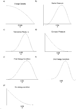
Figure 4: An example of a static wormhole. The graphs indicate: a) $-T^{t}_{\;t}$, b) $T^{x}_{\;x}$, c) $T^{\theta}_{\;\theta}$, d) $T^{A}_{\;A}$, e) $T^{x}_{\;x}-T^{t}_{\;t}$, f) $T^{\theta}_{\;\theta}-T^{t}_{\;t}$, g)$T^{A}_{\;A}-T^{t}_{\;t}$. The functions are plotted from $x=0$ to $x=x_{b}$ (horizontal axis). The vertical scales differ for each plot. These graphs were produced for $D=7$.

In figure 4, we plot the eigenvalues of the stress-energy tensor as well as the corresponding energy conditions. Energy condition violation near the throat is minimal and does not show up in figure 4e. There is also minor WEC violation near the stellar boundary as is evident from figure 4f. This may be eliminated by patching the solution to an intermediate layer of WEC respecting matter and then patching this layer to the vacuum. The transverse pressure, $T^{\theta}_{\;\theta}$, and compact pressure, $T^{A}_{\;A}$ are defined via equations (27b) and (26e) respectively.

At the stellar boundary, the junction conditions of Synge are met and the metric must match the static vacuum. The metric function, $\gamma(x)$, at the boundary is given by the integral of (50):

$$\gamma(x_{b})=\int_{x^{\prime}=0}^{x_{b}}\frac{P(x^{\prime})}{P(x^{\prime})_{,x^{\prime}}}\left\{\left[1+P(x^{\prime})^{2}_{,x^{\prime}}\right]\left[8\pi T^{x}_{\;x}(x^{\prime})-\frac{2}{D-2}\Lambda\right]+\frac{1}{P(x^{\prime})^{2}}\right\}dx^{\prime}+g_{0},$$ (54)

with $g_{0}$ a constant. The metric at the boundary, (54), may be joined to the vacuum of (40) via the identification:

$$\gamma(x_{b}):=2\ln\left[|\kappa_{0}(x_{b}-x_{0})|\right]\;\;\;\mbox{or }\;\;\;|\kappa_{0}|:=\frac{e^{\gamma(x_{b})/2}}{|x_{b}-x_{0}|}$$ (55)

which sets the value of $\kappa_{0}$. This essentially corresponds to a re-scaling of the time coordinate. A similar identification may be utilised to join to the five dimensional vacuum of (37).

For continuity of other metric components at the boundary, it is required that $P(x)$ and $P(x)_{,x}$ be continuous at $x_{b}$. This may most easily be accomplished by fixing one of the many free parameters of the profile curve. The continuity of $P(x)$ yields the condition:

$$\left[\frac{3(D-2)}{2\Lambda}-(x_{b}-x_{0})^{2}\right]^{1/2}=P_{0}+A^{2}x_{b}^{2n}e^{h^{2}(x_{b})}.$$ (56)

Which can easily be satisfied by setting $A$, for example:

$$A^{2}=\frac{\left[\frac{3(D-2)}{2\Lambda}-(x_{b}-x_{0})^{2}\right]^{1/2}-P_{0}}{x_{b}^{2n}}e^{-h^{2}(x_{b})}.$$ (57)

The continuity of $P(x)_{,x}$ requires that

$$\frac{-(x_{b}-x_{0})}{\left[\frac{3(D-2)}{2\Lambda}-(x_{b}-x_{0})^{2}\right]^{1/2}}=2A^{2}x_{b}^{2n}e^{h^{2}(x_{b})}\left[h(x_{b})h(x)_{,x|x=x_{b}}+\frac{n}{x_{b}}\right],$$ (58)

which may be satisfied by setting any one of the remaining free parameters ($x_{0}$, $x_{b}$, $h(x_{b})$ or $\Lambda$). For example, using (57) in (58) one could place a boundary condition on $h(x)$:

$$h(x_{b})h(x)_{,x|x=x_{b}}=\frac{-(x_{b}-x_{0})}{\left[\frac{3(D-2)}{2\Lambda}-(x_{b}-x_{0})^{2}\right]^{1/2}\left\{\left[\frac{3(D-2)}{2\Lambda}-(x_{b}-x_{0})^{2}\right]^{1/2}-P_{0}\right\}}-\frac{n}{x_{b}}.$$ (59)

A simple way to enforce this condition (although by no means the only way) is to set $h(x):=\sqrt{2xF_{0}+(x-x_{b})^{2p}u(x)}$ with $F_{0}$ given by the right-hand-side of (59), $u(x)$ an arbitrary differentiable function and $p$ a sufficiently large constant.

3.2.2 The time-dependent wormhole

We consider here the quasi-static wormhole with the scale factor dictated by (31). Again we wish to study the WEC and begin by expanding $T^{t}_{\;t}$ near the wormhole throat:

$$-8\pi T^{t}_{\;t} \approx \frac{1}{P^{2}_{0}}-\Lambda-\frac{4}{P_{0}}\left[2n^{2}-n\right]A^{2}e^{h^{2}(0)}x^{2n-2}$$ (60)

$$-\frac{8}{P_{0}}\left[2n^{2}+n\right]A^{2}e^{h^{2}(0)}h(0)h(x)_{,x\,|x=0}x^{2n-1}$$

$$+\frac{1}{4}\left\{\frac{1}{2}e^{-\gamma(0)}\left[1-\gamma(x)_{,x|x=0}x\right](D-5)(D-4)\left[\frac{a(t)_{,t}}{a(t)}\right]^{2}+\frac{2(D-5)(D-4)}{a(t)}\right\}$$

$$+\mathcal{O}(x^{2n}).$$

Exactly at the throat, this quantity yields:

$$-8\pi T^{t}_{\;t|x=0} = \frac{1}{P_{0}^{2}}-\Lambda+\frac{1}{8}e^{-\gamma(0)}(D-5)(D-4)\left[\frac{a(t)_{,t}}{a(t)}\right]^{2}+\frac{(D-5)(D-4)}{2a(t)}$$ (61)

$$-\frac{4}{P_{0}}\left[2n^{2}-n\right]A^{2}e^{h^{2}(0)}\,\delta_{n1}.$$

Notice that, although the $\Lambda$ term makes a negative contribution to the energy density of the matter ($\Lambda$ must be positive as dictated by the vacuum), all other terms make positive contributions (for $n>1$) and therefore conditions are quite favourable to have a WEC respecting wormhole. It should be noted that, for $D=5$, the scale factor makes no contribution to $T^{t}_{\;t}$. However, unlike the static case, for $D>5$ we have new time-dependent term which seemingly may be made arbitrarily large and makes a positive contribution to the energy density. We consider below only the cases for $n>1$ since it is easy to check that any energy condition violation is more severe for $n=1$.

To satisfy the boundary condition (43a), we write:

$$\gamma(x)_{,x}=(x_{b}-x)^{l}g(x),$$ (62)

with $l\geq 2$ or $l=1$ and $g(x)$ differentiable but otherwise arbitrary which helps in eliminating singularities. Also, from the equation (26b) we find that

$$8\pi T^{x}_{\;x|x=x_{b}}=\frac{1}{D-2}\Lambda-\left[1+P(x)^{2}_{,x|x=x_{b}}\right]^{-1}\frac{1}{P(x_{b})^{2}}.$$ (63)

Here we have used (62) and the fact that $\gamma(x_{b})\equiv\gamma_{0}$ as required for continuity of the metric at the boundary. From the solution of the vacuum equations, the time-dependent terms in $T^{x}_{\;x}$ give a constant, related to the cosmological constant, at $x=x_{b}$ (or equivalently when $e^{\gamma(x)}=e^{\gamma_{0}}$), this yields the coefficient in the $\Lambda$ term in (63). Therefore, if the profile curve and its first derivative match their corresponding vacuum functions at the boundary, $T^{x}_{\;x}$ will vanish there, satisfying the junction condition (43b). At this point, all junction conditions are met.

As with the static case, there are many ways to enforce continuity of $P(x)$ and $P(x)_{,x}$ at the boundary. Comparing the matter profile curve, (24a) and (24b), with the vacuum (33) one may set, for example,

$$A^{2}= \left\{\left[\frac{D-2}{\Lambda}-(x_{b}-x_{0})^{2}\right]^{1/2}-P_{0}\right\}\frac{e^{-h^{2}(x_{b})}}{x_{b}^{2n}},$$ (64a)

$$h(x)= \sqrt{2xF_{0}+(x-x_{b})^{2p}u(x)},$$ (64b)

with

$$F(x_{b}):=-\frac{(x_{b}-x_{0})\left[\frac{D-2}{\Lambda}-(x_{b}-x_{0})^{2}\right]^{-1/2}}{2\left\{\left[\frac{D-2}{\Lambda}-(x_{b}-x_{0})^{2}\right]^{1/2}-P_{0}\right\}}-\frac{n}{x_{b}}.$$ (65)

Now we wish to investigate the WEC. Consider first the tension generated condition (46a) with (45). Positivity of $-T^{t}_{\;t}$ has already been established and so we next concentrate on negativity of $T^{x}_{\;x}$.

Near the throat we have

$$8\pi T^{x}_{\;x} \approx -\frac{1}{P_{0}^{2}}+\Lambda-\frac{D-4}{4}e^{-\gamma(0)}\left[\frac{1}{2}(D-7)\left(\frac{a(t)_{,t}}{a(t)}\right)^{2}+2\frac{a(t)_{,t,t}}{a(t)}\right]-\frac{(D-5)(D-4)}{2a(t)}$$ (66)

$$+\frac{D-4}{4}e^{-\gamma(0)}x_{b}^{l}g(0)\left[\frac{1}{2}(D-7)\left(\frac{a(t)_{,t}}{a(t)}\right)^{2}+2\frac{a(t)_{,t,t}}{a(t)}\right]x$$

$$+\frac{2n}{P_{0}}x_{b}^{l}g(0)A^{2}e^{h^{2}(0)}x^{2n-1}+\mathcal{O}(x^{2}\mbox{ or greater}),$$

where we have used (62). Therefore, in the vicinity of the throat, a negative radial pressure, or tension, may easily be enforced.

Exactly at the throat, the first energy condition (46a) yields

$$\frac{(D-4)}{2}\left\{e^{-\gamma(0)}\left[\frac{1}{2}\left(\frac{a(t)_{,t}}{a(t)}\right)^{2}-\frac{a(t)_{,t,t}}{a(t)}\right]-\frac{e^{-\gamma(0)/2}}{2}x_{b}^{l}\,|g(0)\frac{a(t)_{,t}}{a(t)}|\right\}\geq 0.$$ (67)

Although it seems likely that the above inequality can be satisfied, it is actually impossible. This is because the scale factor is dictated by the vacuum solution and the term in square brackets is, from (30a), a negative constant. Note that this case is actually worse than the static case since, for the static case, the WEC is respected at the throat.

We next turn our attention to the energy condition (46b). Unlike the previous condition, this condition is generated by positive pressure instead of tension. It is therefore more realistic from an astrophysical point of view.

It is simple to check that the WEC at the throat cannot be satisfied for either (46b) or (46c). To see this recall that both these conditions require $T^{x}_{\;x}\geq 0$ and $T^{t}_{\;t}\leq 0$. Therefore, the linear combination of $8\pi\left[T^{x}_{\;x}-T^{t}_{\;t}\right]$ must be non-negative. Forming this combination using (61) and (66) gives:

$$8\pi\left[T^{x}_{\;x}-T^{t}_{\;t}\right]_{|x=0}=\frac{D-4}{2}e^{-\gamma(0)}\left\{\frac{1}{2}\left[\frac{a(t)_{,t}}{a(t)}\right]^{2}-\frac{a(t)_{,t,t}}{a(t)}\right\}.$$ (68)

As with the previous condition, the quantity in braces is a negative constant. Again, unlike the four dimensional and static cases, a WEC respecting throat is forbidden. Even at points away from the throat, the time dependent terms in $T^{x}_{\;x}-T^{t}_{\;t}$ conspire to yield a negative constant. Therefore, since all energy conditions imply the positivity of some expression which possesses the linear combination $T^{x}_{\;x}-T^{t}_{\;t}$ (a necessary but not sufficient condition), the time dependence tends to impede rather than favour the WEC. This is illustrated in the specific example of figure 5. Figure 5a and b shows that it is possible to have almost everywhere positive energy density and negative radial pressure (as required for (46a)). The graphs in figures 5f-h are plots of the various energy conditions (see figure caption). Positive values indicate WEC respecting regions. These figures show that it is much more difficult than the static case to have WEC respecting regions in the star.

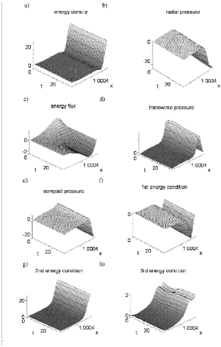
Figure 5: An example of a quasi-static wormhole. The graphs indicate: a) $-T^{t}_{\;t}$, b) $T^{x}_{\;x}$, c) $T^{t}_{\;x}$, d) $T^{\theta}_{\;\theta}$, e) $T^{A}_{\;A}$, f) $T^{x}_{\;x}-T^{t}_{\;t}-2e^{\gamma(x)/2}[1+P(x)_{,x}^{2}]^{-1/2}|T^{t}_{\;x}|$, g) $T^{\theta}_{\;\theta}-T^{t}_{\;t}$, h)$T^{A}_{\;A}-T^{t}_{\;t}$. The functions are plotted from the throat to the boundary ($x$-axis) and over a period of time ($t$-axis). The vertical scales differ for each plot.

Studies have shown that if one introduces time dependence in the four dimensional case, the WEC may be respected for arbitrarily long periods of time [38] - [42]. This is due to the fact that the time dependence may be chosen in such a way as to yield the desired result. The above analysis differs in that the matter field does not possess infinite spatial extent. That is, the global picture is constructed via the introduction of the matter-vacuum boundary. When the models are patched to the vacuum the time dependence of the extra dimensions is now fixed by the vacuum and cannot be chosen arbitrarily. It is this restriction which tends the solution towards WEC violation.

4 Concluding remarks

In this paper we considered static and quasi-static spherically symmetric wormholes with and arbitrary number of extra compact dimensions. The matter models were patched to the vacuum. The vacuum equations were solved and both static and time-dependent vacua were found. Serious restrictions are placed on the wormhole due to the presence of the vacuum-matter boundary and extra dimensions. If one wishes to respect the WEC at the throat in the static case, the extra dimensions place a restriction on the radial size of the wormhole throat. Its radius in the uncompact dimension must be of the order of the size of the compact dimension. The only exception is for $D=5$. For the quasi-static case, the WEC cannot be satisfied at the throat even though seemingly arbitrary time-dependent terms are present in the solution. The WEC can, however, be satisfied throughout most of the stellar bulk in the static case and in isolated regions of the quasi-static star.

References

- [1] L. Flamm, Phys. Z. 17 (1916) 448.
- [2] A. Einstein and N. Rosen, Ann. Phys. 2 (1935) 242.
- [3] H. Weyl, Philosophy of Mathematics and Natural Science, (Princeton Univ. Press, Princeton, 1949).
- [4] J. A. Wheeler, Phys. Rev. 48 (1957) 73.
- [5] C. W. Misner, K .S. Thorne and J. A. Wheeler, Gravitation, (Freeman, San Francisco, 1973).
- [6] V. Dzhunushaliev, Wormhole with quantum throat, gr-qc/0005008.
- [7] R. Garattini, On-line Proceedings of the Marcel Grossman Conference, Rome, Italy, 2000.
- [8] M. Visser, Lorentzian Wormholes-From Einstein to Hawking, (AIP, New York, 1996).
- [9] M. A. Morris and K. S. Thorne, Am. J. Phys. 56 (1988) 395.
- [10] S. W. Hawking, Phys. Rev. D46 (1992) 603.
- [11] J. L. Friedmann, K. Schleich and D. M. Witt, Phys. Rev. Let. 71 (1993) 1486.
- [12] V. Frolov and I. D. Novikov, Phys. Rev. D48 (1993) 1607.
- [13] M. Visser and D. Hochberg, Proc. Haifa Workshop, Haifa, Israel, 1997.
- [14] R. O. Aros and N. Zamorano, Phys. Rev. D56 (1997) 6607.
- [15] D. F. Torres, E. F. Eiroa and G. E. Romero, Mod. Phys. Let. A16 (2001) 1849.
- [16] E. Eiroa, D. F. Torres and G. E. Romero, Mod. Phys. Let. A16 (2001) 973.
- [17] M. Safonova, D. F. Torres and G. E. Romero, Mod. Phys. Let. A16 (2001) 153.
- [18] A. L. Choudhury and P. Hemant, Hadronic J. 24 (2001) 275.
- [19] M. Safonova, D. F. Torres and G. E. Romero, Phys. Rev. D65 (2002) 023001.
- [20] R. C. Myers and M. J. Perry, Ann. Phys. 172 (1986) 304.
- [21] K. A. Bronnikov and V. N. Melnikov, Grav. Cosmol. 1 (1995) 155.
- [22] U. Kasper, M. Rainer and A. Zhuk, Gen. Rel. Grav. 29 (1997) 1123.
- [23] V. N. Melnikov, Proceedings of the 8th Marcel Grossman Meeting, Jerusalem, Israel, 1997.
- [24] S. E. P. Bergliaffa, Mod. Phys. Let. A15 (2000) 531.
- [25] J. Ponce de Leon and N. Cruz, Gen. Rel. Grav. 32 (2000) 1207.
- [26] H. Kim H, S. Moon and J. H. Yee, J.H.E.P. 0202 (2002) 046.
- [27] A. Das and A. DeBenedictis, Prog. Theor. Phys. 108 (2002)119.
- [28] U. Debnath and S. Chakraborty, The study of gravitational collapse model in higher dimensional space-time, gr-qc/0212062.
- [29] N. Arkani-Hamed, S. Dimopoulos and G. Dvali, Phys. Let. B429 (1998) 263.
- [30] I. Antoniadis, N. Arkani-Hamed, S. Dimopoulos and G. Dvali, Phys. Let. B436 (1998) 257.
- [31] N. Arkani-Hamed, S. Dimopoulos and G. Dvali, Phys. Rev. D59 (1999) 086004.
- [32] L. Randall and R. Sundrum, Phys. Rev. Let. 83 (1999) 4690.
- [33] N. Arkani-Hamed, S. Dimopoulos, N. Kaloper and R. Sundrum, Phys. Let. B480 (2000) 193.
- [34] M. Bañados, C. Teitelboim and J. Zanelli, Phys. Rev. Let. 69 (1992) 1849.
- [35] A. DeBenedictis and A. Das, Class. Quant. Grav. 18 (2001) 1187.
- [36] M. S. Morris, K. S. Thorne and U. Yurtsever, Phys. Rev. Let. 61 (1988) 1466.
- [37] P. K. F. Kuhfittig, Am. J. Phys. 67 (1999) 125.
- [38] S. Kar, Phys. Rev. D49 (1994) 862.
- [39] A. Wang and P. S. Letelier, Prog. Theor. Phys. 94 (1995) 137.
- [40] S. Kar and D. Sahdev, Phys. Rev. D53 (1996) 722.
- [41] L. A. Anchordoqui, D. F. Torres, M. L. Trobo and S. E. P. Bergliaffa, Phys. Rev. D57 (1998) 829.
- [42] L. Li, J. Geom. Phys. 40 (2001) 154.
- [43] D. Hochberg and M. Visser, Talk delivered to the Advanced School on Cosmology and Particle Physics, Pensicola Spain, 1999, gr-qc/9901020.
- [44] D. Hochberg and M. Visser, Phys. Rev. Let. 81 (1998) 746.
- [45] S. Hayward, Int. J. Mod. Phys. D8 (1999) 373.
- [46] C. Barceló and M. Visser, Twilight for the energy conditions?, gr-qc/0205066.
- [47] A. G. Riceet al, Astron. J. 116 (1998) 1009.
- [48] S. Perlmutteret al, Astrophys. J. 517 (1999) 565.
- [49] T. A. Roman, Phys. Rev. D47 (1993) 1370.
- [50] S. Weinberg, Gravitation and Cosmology: Principles and Applications of the General Theory of Relativity, (Wiley and Sons, New York. 1972).
- [51] E. Witten, Nucl. Phys. B195 (1982) 481.
- [52] H. Shinkai and T. Shiromizu, Phys. Rev. D62 (2000) 034010.
- [53] J. Geddes, Phys. Rev. D65 (2002) 104015.
- [54] N. Kan and K. Shiraishi, Phys. Rev D66 (2002) 105014.
- [55] G. D. Birkhoff, Relativity and Modern Physics, (Harvard University Press, Boston, 1923).
- [56] K. .A. Bronnikov and V. N. Melnikov, Gen. Rel. Grav. 27 (1995) 465.
- [57] H. J. Schmidt, Grav. Cos. 3 (1997) 185.
- [58] D. Hochberg and M. Visser, Phys. Rev. D56 (1997) 4745.
- [59] F. Kottler, Ann. Phys. 56 (1918) 410.
- [60] J. L. Synge, Relativity: The General Theory, (North-Holland, Amsterdam. 1964).
- [61]