Geodetic Brane Gravity

Abstract

Within the framework of geodetic brane gravity, the Universe is described as a 4-dimensional extended object evolving geodetically in a higher dimensional flat background. In this paper, by introducing a new pair of canonical fields $\{\lambda,P_{\lambda}\}$, we derive the quadratic Hamiltonian for such a brane Universe; the inclusion of matter then resembles minimal coupling. Second class constraints enter the game, invoking the Dirac bracket formalism. The algebra of the first class constraints is calculated, and the BRST generator of the brane Universe turns out to be rank-$1$. At the quantum level, the road is open for canonical and/or functional integral quantization. The main advantages of geodetic brane gravity are: (i) It introduces an intrinsic, geometrically originated, ’dark matter’ component, (ii) It offers, owing to the Lorentzian bulk time coordinate, a novel solution to the ’problem of time’, and (iii) It enables calculation of meaningful probabilities within quantum cosmology without any auxiliary scalar field. Intriguingly, the general relativity limit is associated with $\lambda$ being a vanishing (degenerate) eigenvalue.

I Introduction

Geodetic Brane Gravity (GBG) treats the universe as an extended object (brane) evolving geodetically in some flat background. This idea has been proposed more than twenty years ago by Regge and Teitelboim (’General Relativity a la String’) [1], with the motivation that the first principles which govern the evolution of the entire universe cannot be too different from those which determine the world-line behavior of a point particle or the world-sheet behavior of a string.

Geometrically speaking, the $4$-dimensional curved space-time is a hypersurface embedded within a higher dimensional flat manifold. Following the isometric embedding theorems [4], at most $N=\frac{1}{2}n(n+1)$ background flat dimensions are required to locally embed a general $n$-metric. In particular, for $n=4$, one needs at most a $10$ dimensional flat background. This number can be reduced, however, if the $n$-metric admits some Killing-vector fields.

In Regge and Teitelboim (RT) model, the external manifold (the bulk) is flat and empty, it contains neither a gravitational field nor matter fields. Other models were suggested, where the external manifold is more complicated [19, 20, 21, 22, 23], it may be curved and contain bulk fields which may interact with the brane. RT action, therefore, does not contain bulk integrals, it is only an integral over the brane manifold, which may include the scalar curvature (${\cal R}^{n}$), a constant ($\Lambda$), and some matter Lagrangian (${\cal L}_{matter}$) .

$$S=\int\left(\frac{1}{16\pi G^{n}}{\cal R}^{n}+\Lambda+{\cal L}_{matter}\right)\sqrt{-g^{n}}\,d^{n-1}x\,d\tau$$ (1)

The Geodetic Brane has two parents:

1. General relativity gave the Einstein-Hilbert action, which makes the geodetic brane a gravitational theory.

2. Particle/String theory gave the embedding coordinates $y^{A}(x)$ as canonical fields, and this will lead to geodetic evolution. The $4$ dimensional metric is not a canonical field, it is just being induced by the embedding $g_{\mu\nu}(x)=\eta_{AB}y^{A}_{\,,\mu}(x)y^{B}_{\,,\nu}(x)$.

Due to the fact that the Lagrangian (1) does not depend explicitly on $y^{A}$, but solely on the derivatives through the metric, the geodetic brane equations of motion are actually a set of conservation laws

$$\left[({\cal R}^{\mu\nu}-\frac{1}{2}g^{\mu\nu}{\cal R}-8\pi GT^{\mu\nu})y^{A}_{\,;\mu}\right]_{;\nu}=0.$$ (2)

Eq.(2) splits into two parts, the first is proportional to $y^{A}_{\,,\mu}$ and the second to $y^{A}_{\,;\mu\nu}$. Since the $4$-dimensional covariant derivative of the metric vanishes $g_{\mu\nu;\lambda}=0$, one faces the embedding identity $\eta_{AB}y^{A}_{\,;\lambda}y^{B}_{\,;\mu\nu}=0$. Therefore, the first and second covariant derivatives of $y^{A}$, viewed as vectors in the external manifold, are orthogonal, and each part of Eq.(2) should vanish separately. The part proportional to $y^{A}_{\,,\mu}$ implies that $T^{\mu\nu}_{\,;\nu}=0$. The second part is the geodetic brane equation

$$\left({\cal R}^{\mu\nu}-\frac{1}{2}g^{\mu\nu}{\cal R}-8\pi GT^{\mu\nu}\right)y^{A}_{\,;\mu\nu}=0~{}.$$ (3)

• The matter fields equations remain intact, since the matter Lagrangian depends only on the metric.

• Energy momentum is conserved. This is a crucial result, especially when the Einstein equations are not at our disposal.

• Clearly, every solution of Einstein equations is automatically a solution of the corresponding geodetic brane equations. But the geodetic brane equations allow for different solutions [2]. A general solution of eq.(3) may look like

  $${\cal R}^{\mu\nu}-\frac{1}{2}g^{\mu\nu}{\cal R}-8\pi GT^{\mu\nu}=D^{\mu\nu}$$ (5)

  $$D^{\mu\nu}y^{A}_{\,;\mu\nu}=0\;\;\;D^{\mu\nu}\neq 0$$ (6)

  The non vanishing right hand side of eq.(5) will be interpreted by an Einstein Physicist as additional matter, and since it is not the ordinary $T^{\mu\nu}$ it may labeled Dark Matter [28].

It has been speculated, relying on the structural similarity to string/membrane theory, that quantum geodetic brane gravity may be a somewhat easier task to achieve than quantum general relativity (GR). The trouble is, however, that the parent Regge-Teitelboim [1] Hamiltonian has never been derived!

In this paper, by adding a new non-dynamical canonical field $\lambda$ we derive the quadratic Hamiltonian density of a gravitating brane-universe

$${\cal H}=N^{k}y_{|k}\cdot P-N\frac{8\pi G}{2\sqrt{h}}\left[\left(\frac{\sqrt{h}}{8\pi G}\right)^{2}(\lambda+{\cal R}^{(3)})+P\Theta(\Psi-\lambda I)^{-1}\Theta P\right]~{}.$$ (7)

The derivation of the Geodetic Brane Hamiltonian is done here in a pedagogical way. In section II we translate the relevant geometric objects to the language of embedding. Each object is characterized by its tensorial properties with respect to both the embedding manifold and the brane manifold. We embed the ADM formalism [8] in a higher dimensional Minkowski background, the $4$ dimensional spacetime manifold ($V_{4}$)is artificially separated into a $3$-dimensional space-like manifold ($V_{3}$) and a time direction characterized by the time-like unit vector orthogonal to $V_{3}$. For simplicity we restrict ourselves to $3$-dimensional space-like manifolds with no boundary (either compact or infinite), while the appropriate surface terms should be added when boundaries are present [6].

Section III is the main part of this Paper, where we derive the Hamiltonian. We first look at an empty universe with no matter fields, we present the gravitational Lagrangian density as a functional of the embedding vector $y^{A}(x)$, and derive the conjugate momenta $P_{A}(x)$. Reparametrization invariance causes the canonical Hamiltonian to vanish, (in a similar way to the ADM-Hamiltonian and string theory), and the total Hamiltonian is a sum of constraints. We introduce a new pair of canonical fields $\lambda,P_{\lambda}$ and make the Hamiltonian quadratic in the momenta. Following Dirac’s procedure [7] we separate the constraints into $4$ first-class constraints (reflecting reparametrization invariance), and $2$ second-class constraints (caused by the $2$ extra fields). We define the Dirac-Brackets and eliminate the second-class constraints. The final algebra of the constraints takes the familiar form of a relativistic theory, such as: The relativistic particle, string or membrane.

In section IV we discuss the inclusion of arbitrary matter fields confined to the four dimensional brane. The algebra of the constraints remains unchanged, while the Hamiltonian is simply the sum of the gravitational Hamiltonian and the matter Hamiltonian.

In section V the necessary conditions for classical Einstein gravity are formulated, they are

• $\lambda$ must vanish.

• The total (bulk) momentum of the brane vanishes.

Section VI deals with quantization schemes. We can use canonical quantization by setting the Dirac Brackets to be commutators $\displaystyle{\left\{,\right\}_{D}\longrightarrow i\hbar\left[,\right]}$. The wave-functional of a brane-like Universe [12] is subject to a Virasoro-type momentum constraint equation followed by a Wheeler-deWitt-like equation (first class constraints), the operators are not free, but are constrained by the second class constraints as operator identities. Another quantization scheme is the functional integral formalism, where we use the BFV [15] formulation. The BRST generator [17] is calculated, and the theory turns out to be rank $1$. This resembles ordinary gravity and string theory as oppose to membrane theory, where the rank is the dimension of the underlying space manifold.

Section VII Geodetic Brane Quantum Cosmology is demonstrated. We apply the path integral quantization to the homogeneous and isotropic geodetic brane, within the minisuperspace model. A possible solution to the problem of time arises when one notices that while in GR the only dynamical degree of freedom is the scale factor of the universe, GBQC offers one extra dynamical degree of freedom (the bulk time) that may serve as time coordinate.

Definitions, notations and some lengthy calculations were removed from the main stream of this work and were put in the appendix section.

II The Geometry of Embedding

In this section we will formulate the relevant geometrical objects of the $V_{4}$ and $V_{3}$ manifolds in the language of embedding. Let our starting point be a flat $m$-dimensional manifold ${\cal M}$, with the corresponding line-element being

$$ds^{2}=\eta_{AB}dy^{A}dy^{B}~{}.$$ (8)

• Hypersurfaces : An embedding function $y^{A}(x^{\mu})\;(\mu=0,1,2,3)$ defines the $4$ dimensional hypersurface $V_{4}$ parameterized by the $4$ coordinates $x^{\mu}$. The $V_{4}$ tangent space is spanned by the vectors $y^{A}_{\,,\mu}$. (The $V_{3}$ hypersurface and tangent space are defined in a similar way). The induced $4$-dimensional metric is the projection of $\eta_{AB}$ onto the $V_{4}$ manifold: $g_{\mu\nu}=\eta_{AB}y^{A}_{\,,\mu}y^{B}_{\,,\nu}$. Choosing a time direction $t$ and space coordinates $x^{i}\;(i=1,2,3)$, the induced $4$-dimensional line-element takes the form

  $$ds^{2}=\eta_{AB}(y^{A}_{\,,i}dx^{i}+\dot{y}^{A}dt)(y^{B}_{\,,j}dx^{j}+\dot{y}^{B}dt)~{},$$ (9)

  The various projections of the metric $\eta_{AB}$ onto the space and time directions are denoted as the $3$-metric $h_{ij}$, the shift vector $N_{i}$, and the lapse function $N$

  $$\eta_{AB}y^{A}_{\,,i}y^{B}_{\,,j} = h_{ij}~{},$$ (11)

  $$\eta_{AB}y^{A}_{\,,i}\dot{y}^{B} = N_{i}~{},$$ (12)

  $$\eta_{AB}\dot{y}^{A}\dot{y}^{B} = N_{i}N^{i}-N^{2}~{}.$$ (13)

  These are not independent fields (as in Einstein’s gravity), but are functions of the embedding vector $y^{A}$. Nevertheless, it is a matter of convenience to write down the induced $4$-dimensional line-element in the familiar Arnowitt-Deser-Misner [8] (ADM) form

  $$ds^{2}=-N^{2}dt^{2}+h_{ij}(dx^{i}+N^{i}dt)(dx^{j}+N^{j}dt)~{}.$$ (14)

  The vectors $(\dot{y}^{A},y^{A}_{\,,i})$ span the $4$-dimensional tangent-space of the $V_{4}$ spacetime manifold, while $y^{A}_{\,,i}$ span the $3$-dimensional tangent-space of the $V_{3}$ manifold. Using $h^{ij}$ as the inverse of the $3$-metric $h^{ij}h_{jk}=\delta^{i}_{k}$, one can introduce projections orthogonal to the $V_{3}$ manifold with the operator

  $$\Theta^{A}_{B} = \delta^{A}_{B}-y^{A}_{\,,a}h^{ab}y_{B,b}~{}.$$ (16)

  $$\Theta^{A}_{C}\Theta^{C}_{B} = \Theta^{A}_{B}~{}.$$ (17)

  Now, any vector $v^{A}$ can be separated into the projections tangent and orthogonal to the $V_{3}$ space

  $$v^{A}=v^{A}_{\parallel}+v^{A}_{\perp}=v^{B}y_{B,b}h^{ab}y^{A}_{\,,a}+v^{B}(\delta^{A}_{B}-y^{A}_{\,,a}h^{ab}y_{B,b})~{}.$$ (18)

  An important role is played by the time-like unit vector orthogonal to $V_{3}$-space yet tangent to $V_{4}$-spacetime,

  $$n^{A} \equiv \frac{1}{N}\left(\dot{y}^{A}-N^{i}y^{A}_{\,,i}\right)=\frac{1}{N}\dot{y}^{B}\Theta^{A}_{B}~{},$$ (20)

  $$\eta_{AB}y^{A}_{\,,i}n^{B} = 0~{},$$ (21)

  $$\eta_{AB}n^{A}n^{B} = -1~{}.$$ (22)

  The tangent space of the embedding manifold ${\cal M}$ is spanned by the vectors: $y^{A}_{\,,i}$, $n^{A}$ and $L^{A}_{p}$ ($i=1,2,3\;p=1,..,m-4$). The vectors $L^{A}_{p}$ are chosen to be orthogonal to $y^{A}_{\,,i}$, $n^{A}$ and to each other.

• Curvature : The connections on the underlying $V_{3}$ are $\Gamma^{k}_{ij}=\eta_{AB}y^{A}_{\,,ij}y^{B}_{\,,l}h^{kl}$, this way, the covariant derivative of the $3$-metric vanishes $h_{ij|k}=0$ (the stroke denotes 3-dimensional covariant derivative). As a result, one faces the powerful embedding identity

  $$\eta_{AB}y^{A}_{\,|ij}y^{B}_{\,,k}\equiv 0~{}.$$ (23)

  The vectors $y^{A}_{\,|ij}$ are orthogonal to the $V_{3}$ tangent space and may be written as a combination of $n^{A}$ and $L^{A}_{p}$ [11].

  $$y^{A}_{\,|ij}=n^{A}K_{ij}+L^{A}_{p}\Omega^{p}_{ij}~{}.$$ (24)

  The projection of $y^{A}_{\,|ij}$ in the $n^{A}$ direction is the extrinsic curvature of the $V_{3}$ hypersurface embedded in $V_{4}$

  $$K_{ij}\equiv-\frac{1}{2N}\left(N_{i|j}+N_{j|i}-\frac{\partial h_{ij}}{\partial t}\right)=-\eta_{AB}y^{A}_{\,|ij}n^{B}~{}.$$ (25)

  The coefficient $\Omega^{p}_{ij}$ is the extrinsic curvature of $V_{3}$ with respect to the corresponding normal vector $L^{A}_{p}$.

  The intrinsic curvature of the $V_{3}$ manifold is also related to the second derivative of the embedding functions $y^{A}_{\,|ij}$. The $3$-dimensional Riemann tensor is

  $${\cal R}^{(3)}_{iljk}\equiv\eta_{AB}(y^{A}_{\,|ij}y^{B}_{\,|kl}-y^{A}_{\,|ik}y^{B}_{\,|jl})~{}.$$ (26)

  For convenience we define the $\dot{y}^{A}$-independent symmetric tensor

  $$\Psi^{AB}\equiv(h^{ij}h^{ab}-h^{ia}h^{jb})y^{A}_{\,|ij}y^{B}_{\,|ab}~{}.$$ (27)

  Checking the indices, $\Psi^{AB}$ is a tensor in the embedding manifold, but a scalar in $V_{3}$ space. The trace of $\Psi^{A}_{\,B}$ is simply the $3$-dimensional Ricci scalar ${\cal R}^{(3)}=\eta_{AB}\Psi^{AB}$. Looking at eq.(23), one can easily check that

  $$\Psi^{A}_{\,B}y^{B}_{\,,i}=0~{},$$ (28)

  and $\Psi$ as an operator has at least $3$ eigenvectors with vanishing eigenvalue. Using definitions (27,25), the contraction of $\Psi$ twice with $n^{A}$ is related to the extrinsic curvature

  $$K^{i}_{\,i}K^{j}_{\,j}-K_{ij}K^{ij}=\Psi_{AB}n^{A}n^{B}=\frac{1}{N^{2}}\Psi_{AB}\dot{y}^{A}\dot{y}^{B}~{}.$$ (29)

III Deriving the Hamiltonian

The gravitational Lagrangian density is the standard one

$${\cal L}=\frac{1}{16\pi G}\sqrt{-g}{\cal R}^{(4)}~{}.$$ (30)

Up to a surface term, it can be written in the form

$${\cal L}=\frac{1}{16\pi G}N\sqrt{h}\left[{\cal R}^{(3)}-(K^{i}_{\,i}K^{j}_{\,j}-K_{ij}K^{ij})\right]~{}.$$ (31)

Here, ${\cal R}^{(3)}$ denotes the 3-dimensional Ricci scalar, constructed by means of the 3-metric $h_{ij}$ (11), whereas $K_{ij}$ (25) is the extrinsic curvature of $V_{3}$ embedded in $V_{4}$. Using the tensor $\Psi^{AB}$ (27) one can put the Lagrangian density (31) in the form

$${\cal L}=\frac{\sqrt{h}}{16\pi G}\left[N{\cal R}^{(3)}-\frac{1}{N}\Psi_{AB}\dot{y}^{A}\dot{y}^{B}\right]~{}.$$ (32)

As one can see, the Lagrangian (32) does not involve mixed derivative $\dot{y}^{A}_{\,,i}$ or second time derivative $\ddot{y}^{A}$. The first derivative $\dot{y}^{A}$ appears either explicitly or within $N$. Therefore the Lagrangian

L(y,˙y,y_—i,y_—ij) (33)

is ripe for the Hamiltonian formalism.

The momenta $P_{A}$ conjugate to $y^{A}$ is simply

$$P_{A}(x)\equiv\frac{\delta L}{\delta\dot{y}^{A}(x)}=\frac{\sqrt{h}}{16\pi G}\left\{\left[{\cal R}^{(3)}+\frac{1}{N^{2}}\Psi_{BC}\dot{y}^{B}\dot{y}^{C}\right]\frac{\partial N}{\partial\dot{y}^{A}}-\frac{2}{N}\Psi_{AB}\dot{y}^{B}\right\}~{}.$$ (34)

Using eq.(12,13) to get $\frac{\partial N}{\partial\dot{y}^{A}}=-n_{A}$, while eq.(28) tells us that $\frac{1}{N}\Psi_{AB}\dot{y}^{B}=\Psi_{AB}n^{B}$, the momentum (34) becomes

$$P^{A}=-\frac{\sqrt{h}}{16\pi G}\left\{\left[{\cal R}^{(3)}+n_{B}\Psi^{BC}n_{C}\right]n^{A}+2\Psi^{A}_{\,B}n^{B}\right\}~{}.$$ (35)

The next step should be :”Solve eq.(35) for $\dot{y}^{A}(y,P,y_{|i},y_{|ij})$”. But eq.(35) involves only $n^{A}$, so one would like to solve eq.(35) for $n^{A}(P,y,y_{|i},y_{|ij})$ first, and then to solve eq.(20) for $\dot{y}^{A}$

$$\dot{y}^{A}=Nn^{A}+N^{i}y^{A}_{\,,i}~{}.$$ (36)

This looks innocent but even if one is able to solve eq.(35) for $n^{A}$, any attempt to solve eq.(12) for $N^{i}(n,y,y_{|i})$ and eq.(13) for $N(n,y,y_{|i})$ will lead to a cyclic redefinition of $N^{i}$ and $N$. This situation is similar to other reparametrization invariant theories (such as the relativistic free particle, string theory etc.) and simply means that we have here $4\times V_{3}$ primary constraints

$$\eta_{AB}n^{A}n^{B}+1=0~{},$$ (38)

$$\eta_{AB}y^{A}_{\,,i}n^{B}=0~{}.$$ (39)

The constraints should be written in terms of canonical fields $(y^{A},P_{A})$. So one should solve eq.(35) for $n^{A}(P)$, and then substitute in the above constraints. Any naive attempt to solve eq.(35) for $n^{A}(y,P)$ falls short. The cubic equation involved rarely admits simple solutions. To ’linearize’ the problem we define a new quantity $\lambda$, such that

$$P^{A}=-\frac{\sqrt{h}}{8\pi G}\left(\Psi-\lambda I\right)^{A}_{B}n^{B}~{}.$$ (40)

• Comparing eq.(35) with eq.(40), the definition of $\lambda$ is actually another constraint

  $$n_{A}\Psi^{A}_{\,B}n^{B}+{\cal R}^{(3)}+2\lambda=0~{}.$$ (41)

• An independent $\lambda$ comes along with its conjugate momentum $P_{\lambda}$. $\lambda$ is not a dynamical field therefore one faces another constraint

  $$P_{\lambda}=0~{}.$$ (42)

Assuming $\lambda$ is not an eigenvalue of $\Psi^{A}_{\,B}$, we solve (40) for $n^{A}(\sqrt{h},\Psi,P,\lambda)$ and find

$$n^{A}=-\frac{8\pi G}{\sqrt{h}}\left[\left(\Psi-\lambda I\right)^{-1}\right]^{A}_{\,B}P^{B}~{}.$$ (43)

At this point we have $6\times V_{3}$ primary constraints (38,39,41,42). We will follow Dirac’s way [7] to treat the constrained field theory we have in hand.

First we will write down the various constraints in term of the canonical fields $\left(y^{A}(x),P_{A}(x),\lambda(x),P_{\lambda}(x)\right)$ :

$$\phi_{0} = \frac{8\pi G}{2\sqrt{h}}\left[\left(\frac{\sqrt{h}}{8\pi G}\right)^{2}(\lambda+{\cal R}^{(3)})+P\Theta(\Psi-\lambda I)^{-1}\Theta P\right]\approx 0~{},$$ (45)

$$\phi_{k} = y_{\,|k}\cdot P\approx 0~{},$$ (46)

$$\phi_{4} = P_{\lambda}\approx 0~{},$$ (47)

$$\phi_{5} = \frac{8\pi G}{2\sqrt{h}}\left[\left(\frac{\sqrt{h}}{8\pi G}\right)^{2}+P\Theta(\Psi-\lambda I)^{-2}\Theta P\right]\approx 0~{}.$$ (48)

Notations :

• We use shorthanded notation to simplify the detailed expressions, $F\cdot G\equiv F^{A}G_{A}$ where $F$ and $G$ are vectors in the embedding space, and $P(\Psi-\lambda I)^{-2}P\equiv P_{A}\left[(\Psi-\lambda I)^{-2}\right]^{AB}P_{B}$

• We adopt Dirac’s notation $\phi\approx 0$ for weakly vanishing terms.

• The embedding functions $y^{A}(x)$ and $\lambda(x)$ are scalars in the $V_{3}$ manifold. Their conjugate momenta $P_{A}(x),P_{\lambda}(x)$ are scalar densities of weight $1$. For convenience we normalize all constraints to be scalars in the embedding space, and scalar/vector densities of weight $1$ in $V_{3}$. This way, the Lagrange multipliers are of weight $0$.

• $\phi_{k}$ is based on the constraint (39) but it takes into account the embedding identity (28)

  $$\phi_{k}=y_{\,|k}\cdot P=-\frac{\sqrt{h}}{8\pi G}y_{\,|k}(\Psi-\lambda I)n=\frac{\lambda\sqrt{h}}{8\pi G}y_{\,|k}\cdot n\approx 0~{}.$$ (49)

• $\phi_{5}$ is based on the constraint (38), but we added the projection operator $\Theta$ (17) in front of $P$. This step simplifies the final algebra of the constraints, and brings it to the familiar form of a relativistic theory. Inserting $\Theta$ in front of $P$, is equivalent to adding terms proportional to $\phi_{k}$ (46), since

  $$\Theta^{A}_{B}P^{B}=(\delta^{A}_{B}-y^{A}_{\,,a}h^{ab}y_{B,b})P^{B}=P^{A}-y^{A}_{\,,a}h^{ab}\phi_{b}~{}.$$ (50)

• $\phi_{0}$ is also a combination of the constraints (41),(39) and (38), chosen such that

  $$\frac{\partial\phi_{0}}{\partial\lambda}=\phi_{5}\approx 0~{}.$$ (51)

• See appendix A for the definitions of functional derivatives and Poisson brackets.

In a similar way to other parameterized theories, the canonical Hamiltonian density vanishes

$${\cal H}_{c}=\dot{y}^{A}P_{A}-{\cal L}\approx 0~{}.$$ (52)

This means that the total Hamiltonian is a sum of constraints

$$H=\int d^{3}x\,u^{m}(x)\phi_{m}(x)~{}.$$ (53)

The constraints (III) should vanish for all times, therefore their PB with the Hamiltonian should vanish (at least weakly). This imposes a set of consistency conditions for the functions $u^{m}(x)$

$$\dot{\phi}_{n}(x)=\left\{\phi_{n}(x),H\right\} = \left\{\phi_{n}(x),\int d^{3}z\,u^{m}(z)\phi_{m}(z)\right\}$$ (54)

$$\approx \int d^{3}z\,u^{m}(z)\left\{\phi_{n}(x),\phi_{m}(z)\right\}\approx 0~{}.$$ (55)

The basic Poisson brackets between the constraints are calculated in appendix B, and in general has the form

$$\begin{array}[]{|c|c|c|c|c|}\hline\cr\displaystyle{\left\{\,,\,\right\}\approx}&\phi_{0}(z)&\phi_{l}(z)&\phi_{4}(z)&\phi_{5}(z)\\ \hline\cr\phi_{0}(x)&0&0&0&\frac{8\pi G}{2\sqrt{h}}\,\alpha(x,z)\\ \hline\cr\phi_{k}(x)&0&0&0&\phi_{5,\lambda}\lambda_{|k}\delta(x-z)\\ \hline\cr\phi_{4}(x)&0&0&0&-\phi_{5,\lambda}\delta(x-z)\\ \hline\cr\phi_{5}(x)&-\frac{8\pi G}{2\sqrt{h}}\,\alpha(z,x)&-\phi_{5,\lambda}\lambda_{|k}\delta(x-z)&\phi_{5,\lambda}\delta(x-z)&[F^{i}(x)+F^{i}(z)]\delta_{|i}(x-z)\\ \hline\cr\end{array}$$ (56)

The exact expressions for $\alpha$ and $F^{i}$ appears in appendix B. Now, insert the PB between the constraints (56) into the consistency conditions (55) to determine $u^{m}(x)$

$$\left\{\phi_{4}(x),H\right\} \approx \frac{\partial\phi_{5}}{\partial\lambda}(x)u^{5}(x)\approx 0\Rightarrow u^{5}(x)=0~{},$$ (57)

$$\left\{\phi_{0}(x),H\right\} \approx 0\Rightarrow u^{0}(x)=-N(x)\;\emph{arbitrary}~{},$$ (58)

$$\left\{\phi_{k}(x),H\right\} \approx 0\Rightarrow u^{k}(x)=N^{k}(x)\;\emph{arbitrary}~{},$$ (59)

$$\left\{\phi_{5}(x),H\right\} \approx \int d^{3}z\left[\frac{8\pi G}{2\sqrt{h}}\,\alpha(z,x)N(z)-\phi_{5,\lambda}\lambda_{|k}\delta(x-z)N^{k}(z)+\phi_{5,\lambda}\delta(x-z)u^{4}(z)\right]$$ (61)

$$\Rightarrow u^{4}(x)=N^{k}\lambda_{|k}(x)-\phi_{5,\lambda}^{-1}(x)\int d^{3}z\,{\text{ $\frac{8\pi G}{2\sqrt{h}}$}}\,\alpha(z,x)N(z)~{}.$$

The first class Hamiltonian is then

$$H = \int d^{3}x\left\{\frac{}{}N^{k}\left[y_{|k}\cdot P+\lambda_{|k}P_{\lambda}\right]\right.$$ (62)

$$- N\frac{8\pi G}{2\sqrt{h}}\left[(\frac{\sqrt{h}}{8\pi G})^{2}(\lambda+{\cal R}^{(3)})+P\Theta(\Psi-\lambda I)^{-1}\Theta P\right.$$ (64)

$$~{}~{}~{}\left.\left.+\int d^{3}z\,\alpha(x,z)\phi_{5,\lambda}^{-1}(z)P_{\lambda}(z)\right]\right\}$$

As one can see, at this stage we have in the Hamiltonian $4$ arbitrary functions $N,N^{k}$ (Lagrange multipliers). This means we have $4$ first class constraints reflecting the reparametrization invariance ($4$-dimensional general coordinate transformation)

$$\varphi_{0} = \frac{8\pi G}{2\sqrt{h}}\left[(\frac{\sqrt{h}}{8\pi G})^{2}(\lambda+{\cal R}^{(3)})+P\Theta(\Psi-\lambda I)^{-1}\Theta P\right.$$ (67)

$$+\left.\int d^{3}z\,\alpha(x,z)\phi_{5,\lambda}^{-1}(z)P_{\lambda}(z)\right]\approx 0~{},$$

$$\varphi_{k} = y_{\,|k}P+\lambda_{|k}P_{\lambda}\approx 0~{}.$$ (68)

And we are left with $2$ second class constraints, reflecting the fact that we expanded our phase space with two extra fields $\lambda$ and $P_{\lambda}$

$$\theta_{1}=\phi_{4} = P_{\lambda}\approx 0~{},$$ (70)

$$\theta_{2}=\phi_{5} = \frac{8\pi G}{2\sqrt{h}}\left[\left(\frac{\sqrt{h}}{8\pi G}\right)^{2}+P\Theta(\Psi-\lambda I)^{-2}\Theta P\right]\approx 0~{}.$$ (71)

Using the classical equation of motion for $y^{A}(x)$,

$$\dot{y}^{A}(x)=\left\{y^{A}(x),H\right\}\approx N^{k}y_{|k}-N\frac{8\pi G}{\sqrt{h}}(\Psi-\lambda I)^{-1}P~{},$$ (72)

one can identify the lapse function (13) and the shift vector (12) with $N,N^{k}$ respectively. Thus, recover the nature of the lapse function and the shift vector as Lagrange multipliers only at the stage of the solution to the equation of motion, not as an a priori definition.

We would like to continue along Dirac’s path [7], and use Dirac Brackets (DB) instead of Poisson Brackets (PB). The DB are designed in a way such that the DB of a first class constraint with anything is weakly the same as the corresponding PB, while the DB of a second class constraint with anything vanish identically. Using DB, we actually eliminate the second class constraints (the extra degrees of freedom). The DB are defined as

$$\left\{A,B\right\}_{D}\equiv\left\{A,B\right\}_{P}-\int d^{3}x\int d^{3}z\left\{A,\theta_{m}(x)\right\}_{P}C^{-1}_{mn}(x,z)\left\{\theta_{n}(z),B\right\}_{P}$$ (73)

Where $C^{-1}_{mn}(x,z)$ is the inverse of the second class constraints PB matrix

$\displaystyle C_{mn}(x,z)\equiv\left\{\theta_{m}(x),\theta_{n}(z)\right\}.$

In our case, $C_{mn}(x,z)$ is simply the $2\times 2$ bottom right corner of (56)

$$C_{mn}(x,z)=\left(\begin{array}[]{c|c}0&\displaystyle{-\frac{\partial\phi_{5}}{\partial\lambda}(x)\delta(x-z)}\\ \hline\cr\displaystyle{\frac{\partial\phi_{5}}{\partial\lambda}(x)\delta(x-z)}&\displaystyle{\left[F^{i}(x)+F^{i}(z)\right]\delta_{|i}(x-z)}\end{array}\right)~{}~{}m,n=1,2$$ (74)

When dealing with field theory, the matrix $C_{mn}$ is generally a differential operator, and the inverse matrix is not unique unless one specifies the boundary conditions. We choose ’no-boundary’ as our boundary condition, therefore, integration by parts can be done freely, and the inverse matrix is

$$C^{-1}_{mn}(x,z)=\left(\begin{array}[]{c|c}\displaystyle{\left((\frac{\partial\phi_{5}}{\partial\lambda})^{-2}F^{i}(x)+(\frac{\partial\phi_{5}}{\partial\lambda})^{-2}F^{i}(z)\right)\delta_{|i}(x-z)}&\displaystyle{\left(\frac{\partial\phi_{5}}{\partial\lambda}\right)^{-1}(x)\delta(x-z)}\\ \hline\cr\displaystyle{-\left(\frac{\partial\phi_{5}}{\partial\lambda}\right)^{-1}(x)\delta(x-z)}&0\end{array}\right)$$ (75)

The resulting DB are

$$\left\{A,B\right\}_{D} = \left\{A,B\right\}_{P}+\int d^{3}x\left(\frac{\partial\phi_{5}}{\partial\lambda}\right)^{-2}F^{i}(x)\left[\frac{\delta A}{\delta\lambda(x)}(\frac{\delta B}{\delta\lambda(x)})_{|i}-(\frac{\delta A}{\delta\lambda(x)})_{|i}\frac{\delta B}{\delta\lambda(x)}\right]$$ (77)

$$-\int d^{3}x\left(\frac{\partial\phi_{5}}{\partial\lambda}\right)^{-1}(x)\left[\frac{\delta A}{\delta\lambda(x)}\left\{\phi_{5}(x),B\right\}+\left\{A,\phi_{5}(x)\right\}\frac{\delta B}{\delta\lambda(x)}\right]$$

This way, from now on, one should work with DB instead of PB and take the second class constraints to vanish strongly. This will omit the parts proportional to $P_{\lambda}$ from the first class constraints (67,68) and recover the original form (45,46).

The algebra of the first class constraints takes the familiar form [7] of a relativistic theory

$$\{\phi_{0}(x),\phi_{0}(z)\}_{D} = [h^{ij}\phi_{i}(x)+h^{ij}\phi_{i}(z)]\delta_{|j}(x-z)$$ (79)

$$\{\phi_{0}(x),\phi_{k}(z)\}_{D} = \phi_{0}(z)\delta_{|k}(x-z)$$ (80)

$$\{\phi_{k}(x),\phi_{l}(z)\}_{D} = \phi_{l}(x)\delta_{|k}(x-z)+\phi_{k}(z)\delta_{|l}(x-z)$$ (81)

The final first class Hamiltonian of a bubble universe is

H = ∫d3x{Nky—k⋅P -N8πG2h[ (h8πG)2(λ+ R(3)) + PΘ(Ψ- λI)-1ΘP ]} (82)

At this stage, we have a first class Hamiltonian composed of four first class constraints, and accompanied with two second class constraints. The algebra of the first class constraints is the familiar algebra of other relativistic theories. Before moving on to quantization schemes we would like to study two more classical aspects: what happens if the action includes brane matter fields, and what is the relation between Einstein’s solutions to the geodetic brane solutions.

IV Inclusion of Matter

The inclusion of matter is done by adding the action of the matter fields to the gravitational action

$$S=\int d^{4}x\left[\sqrt{-g}\frac{1}{16\pi G}{\cal R}^{(4)}+{\cal L}_{m}\right]~{}.$$ (83)

The matter Lagrangian density depends in general on some matter fields, but also on the $4$-dimensional metric $g_{\mu\nu}$. The dynamics of the matter fields is actually not affected by the exchange of the canonical fields from $g_{\mu\nu}$ to $y^{A}$, and one expects the same equations of motion or the same ’matter’ Hamiltonian density. On the other hand the momenta $P_{A}$ gets a contribution from the matter Lagrangian

$$\Delta P_{A}=\frac{\delta{\cal L}_{matter}}{\delta\dot{y}^{A}}=\sqrt{h}\left[T_{nn}n^{A}-h^{ij}T_{ni}y^{A}_{\,,i}\right]~{}.$$ (84)

This contribution depends on the various projections of the energy-momentum tensor

$$T^{\mu\nu}\equiv\frac{2}{\sqrt{-g}}\frac{\delta{\cal L}_{matter}}{\delta g_{\mu\nu}}~{}.$$ (85)

$T_{nn}$ is the matter energy density, or the projection of the energy-momentum tensor twice onto the $n^{A}$ direction $T_{nn}\equiv\left(T^{\mu\nu}y^{A}_{\,,\mu}y^{B}_{\,,\nu}\right)n_{A}n_{B}$. While in $T_{ni}$ the energy-momentum tensor is projected once onto the $n^{A}$ direction and once onto the $V_{3}$ tangent space. $T_{ni}\equiv\left(T^{\mu\nu}y^{A}_{\,,\mu}y^{B}_{\,,\nu}\right)n_{A}y_{B,i}$. See appendix C for some examples of matter Lagrangians, Hamiltonians and the corresponding energy-momentum tensor projections.

The momenta $P_{A}$ (35) is now changed to

$$P^{A}=-\frac{\sqrt{h}}{16\pi G}\left\{\left[{\cal R}^{(3)}+n_{B}\Psi^{BC}n_{C}-16\pi GT_{nn}\right]n^{A}+2\Psi^{A}_{\,B}n^{B}+16\pi GT_{ni}h^{ij}y^{A}_{\,,i}\right\}$$ (86)

Following the same logic that lead us from Eq.(35) to the introduction of $\lambda$ (41), we will define $\lambda$ as

$$n_{A}\Psi^{A}_{\,B}n^{B}+{\cal R}^{(3)}-16\pi GT_{nn}+2\lambda=0~{}.$$ (87)

The effects of matter are thus $\lambda\rightarrow\lambda+8\pi GT_{nn}$, $P^{A}\rightarrow P^{A}-\sqrt{h}T_{ni}h^{ij}y^{A}_{\,,i}$ but $\Theta P$ is unchanged. The constraints are modified as follows

$$\phi_{0} \longrightarrow \phi_{0}-\sqrt{h}T_{nn}$$ (88)

$$\phi_{k} \longrightarrow \phi_{k}+\sqrt{h}T_{nk}$$ (89)

Thus the Hamiltonian is changed to

$$H_{G}\longrightarrow H_{G}+\int d^{3}x\sqrt{h}[N^{k}T_{nk}+NT_{nn}]=H_{G}+H_{m}~{},$$ (90)

Where $H_{m}$ is the matter Hamiltonian, calculated in terms of the matter fields alone as shown in appendix C. The algebra of the constraints (III) remains unchanged under the inclusion of matter, where the PB now include the derivatives with respect to matter fields as well.

V The Einstein Limit

In some manner Regge-Teitelboim gravity is a generalization of Einstein gravity. Any solution to Einstein equations is also a solution to RT equations (3). We will derive here the necessary conditions for a RT-solution to be an Einstein-solution.

• First, we use a purely geometric relation

  $$2G_{nn}={\cal R}^{(3)}+n^{B}\Psi_{BC}n^{C}~{},$$ (91)

  where $G_{nn}$ is the Einstein tensor twice projected onto the $n^{A}$-direction. The constraint associated with the introduction of $\lambda$ (87) is

  $$-2\lambda={\cal R}^{(3)}+n^{B}\Psi_{BC}n^{C}-16\pi GT_{nn}=2(G_{nn}-8\pi GT_{nn})~{}.$$ (92)

  The Einstein solution of the equation is therefore associated with

  $$\framebox{{\hbox{\displaystyle{\lambda= 0}}}}~{}.$$ (93)

  As was shown in Eq.(28), $\Psi$ has a degenerate vanishing eigenvalue. Therefore Einstein case with $\lambda=0$, will not allow for the essential $(\Psi-\lambda I)^{-1}$. One can not impose $\lambda=0$ as an additional constraint (as was proposed by RT [1]), but only look at it as a limiting case.

• Second, we use the projection of the Einstein tensor once onto the $n^{A}$-direction and once onto the $V_{3}$ tangent space $G_{ni}$

  $$G_{ni}h^{ij}y^{A}_{\,,j}=-\Psi^{A}_{\,B}n^{B}-\left(y^{A}_{\,,j}(Kh^{ij}-K^{ij})\right)_{|i}~{},$$ (94)

  in eq.(86) and put the momentum $P^{A}$ in the form

  $$P^{A}=-\frac{\sqrt{h}}{8\pi G}\left[(G_{nn}-8\pi GT_{nn})n^{A}-(G_{ni}-8\pi GT_{ni})h^{ij}y^{A}_{\,,j}+\left(y^{A}_{\,,j}(Kh^{ij}-K^{ij})\right)_{|i}\right]~{}.$$ (95)

  It is clear that if Einstein equations $G_{nn}=8\pi GT_{nn}$ and $G_{ni}=8\pi GT_{ni}$ are both satisfied, the momentum $P_{A}$ makes a total derivative such that

  $$\oint d^{3}xP_{A}=0~{}.$$ (96)

  The total momentum $\oint d^{3}xP_{A}$ is a conserved Noether charge since the original Lagrangian does not depend explicitly on $y^{A}$

  $$\mu^{A}\equiv\oint d^{3}xP^{A}={\hbox{ const.}}~{}.$$ (97)

  The universe, as an extended object, is characterized by the total momentum $\mu^{A}$. The necessary condition for an Einstein-solution is a vanishing $\mu^{A}$.

  $$\framebox{{\hbox{\displaystyle{ \mu^{A} \equiv\oint d^{3}xP^{A} = 0 }}}}~{}.$$ (98)

• The condition (98) simply tells us that the total ’bulk’ momentum of the universe vanishes. This motivates us to use a new coordinate system for the embedding, namely, the ’center of mass frame’ $+$ ’relative coordinates’. As relative coordinates we will use the derivatives $y^{A}_{\,,i}\,$. This has a direct relation to the metric and therefore, we expect the equation of motion to resemble Einstein’s equations. The new system and the calculations appear in appendix D.

VI Quantization

The treatment so far was classical, but the derivation of the Hamiltonian and the construction of the various constraints are the ingredients one needs for quantization. In the following sections we will describe two quantization schemes, canonical quantization and functional integral quantization.

A Canonical Quantization

Dirac’s procedure leads us towards the canonical quantization of our constrained system. The following recipe was constructed by Dirac [7] for quantizing a constrained system within the Schrodinger picture

• Represent the system with a state vector (wave functional) .

• Replace all observables with operators.

• Replace DB with commutators, $\displaystyle{\left\{,\right\}_{D}\longrightarrow i\hbar\left[,\right]}$

• First class constraints annihilate the state vector.

• Second class constraints represent operator identities.

• Since the commutator is ill defined for fields at the same space point, one must place all momenta to the right of the constraint.

• First class constraints must commute with each other. This ensures consistency, and may call for operator ordering within the constraint.

In our case, we can use the coordinate representation. The state vector is represented by a wave functional $\Phi[y]$. The DB (commutator) between $y^{A}$ and $P_{B}$ is canonical, therefore, these operators can be represented in a canonical way

$$\hat{y}^{A}(x)\Rightarrow y^{A}(x)$$ (99)

$$\hat{P}_{A}(x)\Rightarrow-i\hbar\frac{\delta}{\delta y^{A}(x)}$$ (100)

The operator $\hat{P_{\lambda}}$ vanishes identically. The DB of $\lambda$ with $y^{A}$,$P_{B}$ are not canonical, therefore the operator $\hat{\lambda}$ must be expressed as a function of $\hat{y^{A}}$,$\hat{P_{B}}$ . This can be done with the aid of the second class constraint (71).

The first class constraints as operators must annihilate the wave functional. These constraints are recognized as

1. The momentum constraint (68)

   $$-i\hbar y^{A}_{\,|k}\frac{\delta\Phi}{\delta y^{A}}=0~{},$$ (101)

   which simply means that the wave functional is a $V_{3}$ scalar and does not change its value under reparametrization of the space coordinates. This can be shown if one takes an infinitesimal coordinate transformation

   $$x^{k} \longrightarrow x^{k}+\epsilon^{k}~{},$$ (102)

   $$y^{A}(x) \longrightarrow y^{A}(x)+\epsilon^{k}y^{A}_{\,|k}(x)~{},$$ (103)

   $$\Phi[y] \longrightarrow \Phi[y]+\epsilon^{k}y^{A}_{\,|k}\frac{\delta\Phi[y]}{\delta y^{A}}~{}.$$ (104)

   The wave functional is unchanged if and only if the momentum constraint holds.

2. The other constraint is the Hamiltonian constraint, and up to order ambiguities, the equation is the analog to the Wheeler de-Witt equation

   $$\frac{8\pi G}{2\sqrt{h}}\left[\left(\frac{\sqrt{h}}{8\pi G}\right)^{2}(\hat{\lambda}+{\cal R}^{(3)})(x)-\hbar^{2}\left((\Psi-\hat{\lambda}I)^{-1}\right)^{AB}(x)\frac{\delta^{2}}{\delta y^{A}(x)\delta y^{B}(x)}\right]\Phi[y]=0~{}.$$ (105)

   It is accompanied however, with the operator identity

   $$\frac{8\pi G}{2\sqrt{h}}\left[\left(\frac{\sqrt{h}}{8\pi G}\right)^{2}+\hat{P}\Theta(\Psi-\hat{\lambda}I)^{-2}\Theta\hat{P}\right]=0$$ (106)

B Functional Integral Quantization

Calculating functional integrals for a constrained system is not new. This was done for first class constraints by BFV [15], And was generalized for second class constraints by Fradkin and Fradkina [16].

The first step is actually a classical calculation, that is, calculating the BRST generator [17]. For this calculation we will adopt the following notations:

• The set of canonical fields will include the Lagrange multipliers $N^{\mu}=(N,N^{i})$ that is $Q^{A}=\left(y^{A},\lambda,N^{\mu}\right)^{T}$, and the corresponding conjugate momenta $\Pi_{A}=(P_{A},P_{\lambda},\pi_{\mu})$. The Lagrange multipliers are not dynamical, therefore, the conjugate momenta must vanish. This doubles the number of first class constraints $G_{a}=(\pi_{\mu},\phi_{\nu})$.

• For each constraint we introduce a pair of fermionic fields $\eta^{a}=\left(\rho^{\mu},c^{\mu}\right)^{T}$, and the conjugate momenta ${\cal P}_{a}=(\bar{c}_{\nu},\bar{\rho}_{\nu})$. (In our case, all constraints are bosonic, therefore the ghost fields are fermions).

• Each index actually represent a discrete index and a continuous index, for example, $y^{A}\equiv y^{A}(x)$. The summation convention is then generalized to sum over the continuous index as well

  $$N^{\mu}\phi_{\mu}\equiv\int d^{3}xN^{\mu}(x)\phi_{\mu}(x)~{}.$$ (107)

• We use Dirac Brackets as in (77), but the Poisson Brackets are generalized to include bosonic and fermionic degrees of freedom

  $$\left\{L,R\right\}=\frac{\partial^{r}L}{\partial q^{A}}\frac{\partial^{l}R}{\partial p_{A}}-(-1)^{n_{L}n_{R}}\frac{\partial^{r}R}{\partial q^{A}}\frac{\partial^{l}L}{\partial p_{A}}~{}.$$ (108)

  Where $(q,p)$ is the set of canonical fields including the fermionic fields. $r,l$ denote right and left derivatives

  $$dR=\frac{\partial^{r}R}{\partial q}dq=dq\frac{\partial^{l}R}{\partial q}~{}.$$ (109)

  And the fermionic index is

  $$n_{R}=\left\{\begin{array}[]{l l}0&$if R is a boson$\\ 1&$if R is a fermion$\end{array}\right.$$ (110)

Let us now calculate the structure functions of the theory. The first order structure functions are defined by the algebra of the constraints $\{G_{a},G_{b}\}_{D}=G_{c}U^{c}_{ab}$. It is only the original constraints, (not the multipliers momenta), that have non vanishing structure functions (III).

$$\left\{\left(\begin{array}[]{c}\pi_{\mu}(x)\\ \phi_{\mu}(x)\end{array}\right),\left(\pi_{\nu}(z),\phi_{\nu}(z)\right)\right\}_{D}=\left(\begin{array}[]{c c}0&0\\ 0&\int d^{3}w\,\phi_{\lambda}(w)U^{\lambda}_{\mu\nu}(x,z,w)\end{array}\right),$$ (111)

and the relevant first order structure functions are

$$U^{\lambda}_{\mu\nu}(x,z,w)=\left[\delta^{0}_{\mu}\delta^{0}_{\nu}h^{\lambda k}\left(\delta(w-x)+\delta(w-z)\right)+\delta^{\lambda}_{\mu}\delta^{k}_{\nu}\delta(w-z)+\delta^{k}_{\mu}\delta^{\lambda}_{\nu}\delta(w-x)\right]\delta_{,k}(x-z)$$ (112)

(Generally, one should also look at $\{H_{0},G_{a}\}_{D}=G_{b}V^{b}_{a}$, but here $H_{0}=0$). The second order structure functions are defined by the Jacobi identity ${{\cal A}(\{\{G_{a},G_{b}\}_{D},G_{c}\}_{D})=0}$, where ${\cal A}$ means antisymmetrization. Using the first order functions (112) one gets ${{\cal A}(G_{d}[\{U^{d}_{ab},G_{c}\}_{D}+U^{d}_{ec}U^{e}_{ab}])=0}$. This equation is satisfied if and only if the expression in the square brackets is again a sum of constraints

$${\cal A}(\{U^{d}_{ab},G_{c}\}_{D}+U^{d}_{ec}U^{e}_{ab})=G_{f}U^{fd}_{abc}.$$ (113)

The second order structure functions $U^{fd}_{abc}$ are antisymmetric on both sets of indices. In our case, the second order structure functions vanish, and the theory is of rank $1$. This resembles ordinary gravity and string theory as oppose to membrane theory, where the rank is the dimension of the underlying space manifold. The BRST generator of a rank $1$ theory is given by $\Omega=G_{a}\eta^{a}+\frac{1}{2}{\cal P}_{c}U^{c}_{ab}\eta^{b}\eta^{a}$. Here it is

$$\Omega=\int d^{3}x[\pi_{\mu}\rho^{\mu}+\phi_{\mu}c^{\mu}+h^{kl}\bar{\rho}_{k}c^{0}_{\,,l}c^{0}+\bar{\rho}_{\mu}c^{\mu}_{\,,k}c^{k}](x).$$ (114)

The main theorem of BFV [15] is that the following functional integral does not depend on the choice of the gauge fixing Fermi function $\Psi$ :

$$Z_{\Psi}=\int{\cal D}Q^{A}{\cal D}\Pi_{A}{\cal D}\eta^{a}{\cal D}{\cal P}_{a}\,M\,\exp[i\int dt(\Pi_{A}\dot{Q}^{A}+{\cal P}_{a}\dot{\eta}^{a}-H_{\Psi})]~{}.$$ (115)

Where $M=\delta(\theta_{1})\delta(\theta_{2})(\det C_{mn})^{1/2}$ is taking care of the second class constraints, and, since the canonical Hamiltonian vanishes, $H_{\Psi}=-\{\Psi,\Omega\}_{D}$.

The determinant of $C_{mn}$ for compact space manifolds, is calculated in a simple way in appendix E.

VII An Example: Geodetic Brane Quantum Cosmology

In the following example we would like to implement GBG to cosmology, and in particular to quantum cosmology. Detailed examples and calculations can be found in [27, 29], here we will just focus on global characteristics of the Feynman propagator for a geodetic brane within the minisuperspace model. Attention will be given to the differences between ’Geodetic Brane Quantum Cosmology’ and the standard ’Quantum Cosmology’.

The standard and simple way to describe the cosmological evolution of the universe is to assume that on large scales the universe is homogeneous and isotropic. The geometry of such a universe is described by the Friedman-Robertson-Walker (FRW) metric

$$ds^{2}=-N^{2}(t)dt^{2}+a^{2}(t)d\Omega_{3}^{2},$$ (116)

where $N(t)$ is the lapse function, $a(t)$ is the scale factor of the universe, and

$$d\Omega_{3}^{2}=d\psi^{2}+\chi^{2}(\psi)d\Omega_{2}^{2}$$ (117)

is the line element of the $3$ dimensional spacelike hypersurface which is assumed to be homogeneous and isotropic. $d\Omega_{2}^{2}$ is the usual line element on a $2$ sphere, and $\chi(\psi)=\sin\psi\,/\,\psi\,/\,\sinh\psi$ if the $3$ space is closed, flat or open respectively. In General Relativity, the components of the metric are the dynamical fields, the lapse function $N(t)$ is actually a Lagrange multiplier, and the only dynamical variable is the scale factor $a(t)$. This model is called minisuperspace, since, the infinite number of degrees of freedom in the metric is reduced to a finite number. The remnant of general coordinate transformation invariance, is time reparameterization invariance, that is, the arbitrariness in choosing $N(t)$. The usual and most convinient gauge is $N=1$.

In GBG the situation is quite different. First, one has to embed the FRW metric (116) in a flat manifold. The minimal embedding of a FRW metric calls for one extra dimension. We will work here, for simplicity, with the closed universe $\chi=\sin\psi$. The embedding in a flat Minkowski spacetime with the signature $(-,+,+,+,+)$, is given by [5]

$$y^{A}=\left(\begin{array}[]{l}T(t)\\ a(t)z^{I}(x)\end{array}\right)\;\;\;z^{I}=\left(\begin{array}[]{l}\sin\psi\sin\theta\cos\phi\\ \sin\psi\sin\theta\sin\phi\\ \sin\psi\cos\theta\\ \cos\psi\end{array}\right)~{}.$$ (118)

The lapse function is given by $N(t)=\sqrt{\dot{T}^{2}-\dot{a}^{2}}$, it is not a Lagrange multiplier, but it depends on the two dynamical variables: the scale factor $a(t)$ and the external timelike coordinate $T(t)$. Time reparameterization invariance is, naturally, an intrinsic feature of $\sqrt{\dot{T}^{2}-\dot{a}^{2}}\,dt$, but, no gauge fixing is allowed here, since both $T(t)$ and $a(t)$ are dynamical. The gravitational Lagrangian (32), after integrating over the spatial manifold is

$$L=\sigma\left(3Na-\frac{3a\dot{a}^{2}}{N}\right).$$ (119)

$\sigma=\frac{2\pi^{2}}{8\pi G}$ is a scaling factor, for convinience we will set $\sigma=1$. The key for quantization is of course the Hamiltonian. One can derive the Hamiltonian directly from the Langrangian (119), or, to use the ready made Hamiltonian (82) and just insert the ’minimized’ expressions for the embedding vector, and the conjugate momenta.

A Minisuperspace Hamiltonian

The first step is to introduce the coordinates and conjugate momenta. The general embedding vector $y^{A}$ is replaced by the dynamical degrees of freedom $a(t)$ and $T(t)$, while the spatial dependence is forced by the expression (118). It is expected that the conjugate momenta will have two degrees of freedom $P_{a}(t),P_{T}(t)$, the delicate issue is the spatial dependence of the momenta. Our choice is

$$P_{A}=\left(\begin{array}[]{l}P_{T}(t)\\ P_{a}(t)z^{I}(x)\end{array}\right)\cdot\frac{\sin^{2}\psi\sin\theta}{8\pi G}~{},$$ (120)

the factor $\sin^{2}\psi\sin\theta$ was inserted in order to keep the momenta a $3$-dimensional vector density. The spatial dependence is through $z^{I}(x)$ such that the momentum constraint (46) vanishes strongly. And, the normalization is $\int d^{3}x\,\dot{y}^{A}p_{A}=\sigma(\dot{a}P_{a}+\dot{T}P_{T})$. In addition, we set $\lambda=\lambda(t)$ and $P_{\lambda}=P_{\lambda}(t)\frac{\sin^{2}\psi\sin\theta}{8\pi G}$.

Inserting these expressions into the constraints (III) and integrating over spatial coordinates, one is left with one first class constraint

$$\varphi=\frac{1}{2}\left(6a+a^{3}\lambda+\frac{P_{T}^{2}}{a^{3}\lambda}+\frac{P_{a}^{2}}{6a-a^{3}\lambda}+\alpha P_{\lambda}\right)\approx 0~{},$$ (121)

and two second class constraints

$$\theta_{1} = P_{\lambda}\approx 0$$ (122)

$$\theta_{2} = \frac{1}{2}\left(a^{3}-\frac{P_{T}^{2}}{a^{3}\lambda^{2}}+\frac{a^{3}P_{a}^{2}}{(6a-a^{3}\lambda)^{2}}\right)\approx 0~{}.$$ (123)

The Dirac brackets (77) are defined as

$$\left\{A,B\right\}_{D} = \left\{A,B\right\}_{P}-\left(\frac{P_{T}^{2}}{a^{6}\lambda^{3}}+\frac{a^{6}P_{a}^{2}}{(6a-a^{3}\lambda)^{3}}\right)^{-1}\left[\frac{\partial A}{\partial\lambda}\{\theta_{2},B\}+\{A,\theta_{2}\}\frac{\partial B}{\partial\lambda}\right]$$ (124)

and the minisuperspace Hamiltonian is

$$H=\frac{-N}{2}\left(6a+a^{3}\lambda+\frac{P_{T}^{2}}{a^{3}\lambda}+\frac{P_{a}^{2}}{6a-a^{3}\lambda}+\alpha P_{\lambda}\right)~{},$$ (125)

We would like to focus on the Feynman propagator [14] $K(a_{f},T_{f},t_{f};a_{i},T_{i},t_{i})$ for the empty geodetic brane universe. Although the empty universe is a non-realistic model for our universe, the calculation of the propagator is simple and it demonstrates some of the main features and advantages of Geodetic Brane Quantum Cosmology over the standard quantum cosmology models. This propagator is the probability amplitude that the universe is in $(a_{f},T_{f})$ at time $t_{f}$, and it was in $(a_{i},T_{i})$ at time $t_{i}$. We will use a modified version of BFV integral offered by Senjanovic [18], where the ghosts and multipliers were integrated out.

$$K(a_{f},T_{f},t_{f};a_{i},T_{i},t_{i}) = \int d\mu\,\exp\left[2\pi i\int_{t_{i}}^{t_{f}}dt(\dot{a}P_{a}+\dot{T}P_{T}+\dot{\lambda}P_{\lambda})\right]$$ (126)

$$d\mu = da\,dP_{a}\,dT\,dP_{T}\,d\lambda\,dP_{\lambda}\,\delta(\varphi)\,\delta(\chi)\,|\{\chi,\varphi\}|\,\delta(\theta_{1})\,\delta(\theta_{2})\,|\det(\{\theta_{m},\theta_{n}\})|^{1/2}$$ (127)

This propagator is calculated in phase space, where the measure is the Liuville measure $dx\,dp$. In addition, the measure $d\mu$ enforces the constraints (first and second class) by delta functions, it includes an arbitrary gauge fixing function $\chi$, the determinants of the Poisson brackets between first class constraints and the gauge fixing function and the determinants of the Poisson brackets between second class constraints. Attention should be given to the following issues:

• The canonical Hamiltonian vanishes, therefore it is absent in the action.

• The boundary conditions for the propagator determine the values of $a_{f},T_{f},a_{i},T_{i}$, but not the value of $\lambda$ nor the values of the momenta. Therefore, the momenta and $\lambda$ must be integrated over at the initial point.

• The gauge fixing function $\chi$, although arbitrary, must be chosen such that it does not violate the boundary conditions nor the constraints. In addition, the Poisson brackets $\{\chi,\varphi\}$ must not vanish.

• The determinant of the second class constraints Poisson brackets is simply

  $$|\det(\{\theta_{m},\theta_{n}\})|^{1/2}=\left|\frac{\partial\theta_{2}}{\partial\lambda}\right|=\left|\frac{P_{T}^{2}}{a^{3}\lambda^{3}}+\frac{a^{6}P_{a}^{2}}{(6a-a^{3}\lambda)^{3}}\right|$$ (128)

• Our convention here is $\sigma=1$ and Planck constant $h=1$ ($\hbar=\frac{1}{2\pi}$).

• In cases where matter is included, the inclusion of matter will affect in a few places. The action will include terms like $\dot{\phi}\pi$, an integration over matter fields and momenta will be added, and the first class constraint will have a contribution which is simply the matter Hamiltonian $\varphi\longrightarrow\varphi+H_{m}(a,\phi,\pi)$. All other constraints remain intact.

The calculation of the propagator (127) is carried out in a simple way following Halliwell [13], and the final propagator takes the form

$$K_{\pm}(a_{f},T_{f};a_{i},T_{i})=\int d\omega\,\exp\left[2\pi i\omega(T_{f}-T_{i})\mp 2\pi i\omega^{2}\left(F(x_{f})-F(x_{i})\right)\right]$$ (129)

The index of $K_{\pm}$ and the $\mp$ in the exponent refers to the expanding/contracting scale factor. $\omega$ is the conserved bulk energy (the momentum conjugate to the bulk time coordinate $T$). Since the value of $\omega$ is not fixed at the initial condition, one must integrate over $\omega$. One should notice according to eq.(98) that the Einstein solution is assiciated with $\omega=0$. The function $F(x)$ is given by

$$F(x)=\left\{\begin{array}[]{ll}\frac{1}{12}\left[3\text{Arcsin}x+\sqrt{1-x^{2}}(4x^{5}+2x^{3}-3x)\right]&|x|\leq 1\\ \text{sgn}(x)\frac{\pi}{8}-\frac{i}{12}\left[3\text{sgn}(x)\text{Arccosh}|x|-\sqrt{x^{2}-1}(4x^{5}+2x^{3}-3x)\right]&1<|x|\end{array}\right.$$ (130)

Where $x=(\frac{3a}{\omega})^{1/3}$.

Let us now examine the properties of the propagator (129). Actually, the propagator is independent of the internal time parameter $t$ (a common character of all parameterized theories), and depends exclusively on the value of $a$ and $T$ at the boundaries.

• The most basic characteristic of a propagator is the possibility to propagate from an initial state to a final state through an intermidiate state. For example, the propagator for a non-relativistic particle is $K(x_{3},t_{3};x_{1},t_{1})=\int dx_{2}K(x_{3},t_{3};x_{2},t_{2})K(x_{2},t_{2};x_{1},t_{1})$. At the intemidiate time $t_{2}$, one must integrate over $x_{2}$. It is clear that there is no integration over $t_{2}$, $t$ is the evolution parameter, it must be monotonic $t_{3}>t_{2}>t_{1}$, and integration over $t_{2}$ makes no sense. Another characteristic of the propagator is $\lim_{t_{2}\rightarrow t_{1}}K(x_{2},t_{2};x_{1},t_{1})=\delta(x_{2}-x_{1})$. The situation with parameterized theories is quite different. The propagator is independent of the internal time, and integration over all dynamical variable diverges. The solution is, usually, to let one of the dynamical variables as ’time’, and integrate only over the other variables.

  The question is: How does the propagator (129) behaves at the intermidiate point ? What is the relevant evolution parameter and what integrations should be made ? One can check that if $a$ is taken to be the monotonic evolution parameter and integration over $T$ at the intermidiate point is done, then the propagator (129) is well behaved.

  $$K(a_{3},T_{3};a_{1},T_{1}) = \int dT_{2}\int d\omega\,e^{2\pi i[\omega(T_{3}-T_{2})-\omega^{2}(F(x_{3})-F(x_{2}))]}\int d\bar{\omega}\,e^{2\pi i[\bar{\omega}(T_{2}-T_{1})-\bar{\omega}^{2}(F(\bar{x}_{2})-F(\bar{x}_{1}))]}$$ (131)

  $$= \int d\omega\,e^{2\pi i[\omega(T_{3}-T_{1})-\omega^{2}(F(x_{3})-F(x_{1}))]}$$ (132)

  $$K(a_{1},T_{2};a_{1},T_{1}) = \int d\omega\,e^{2\pi i\omega(T_{2}-T_{1})}=\delta(T_{2}-T_{1})$$ (133)

  This cannot be done within the standard quantum cosmology models, since there, the only dynamical variable is the scale factor $a$. Such a propagator of only one variable contains no information, it can tell that the varible is monotonic. The common solution in standard quantum cosmology is to add another dynamical variable such as a scalar field and to use one of them as the evolution parameter. Here we see one of the main advantages of Geodetic Brane Quantum Cosmology over the standard models, the problem of time has an intrinsic solution as we have one extra degree of freedom which serves as ’time’.

• The most general wave function that can be generated using the propagator (129) is

  $$\Psi(a,T)=\int d\omega\,e^{2\pi i\omega T}\left[A(\omega)e^{-2\pi i\omega^{2}F(x)}+B(\omega)e^{2\pi i\omega^{2}F(x)}\right]~{}.$$ (134)

  One can verify that the wave function (134) (and the propagator (129)) satisfy the corresponding WDW equation

  $$\hbar^{2}\left[-\xi(x)\frac{\partial}{\partial a}\left(\frac{1}{\xi(x)}\frac{\partial}{\partial a}\right)+\xi^{2}(x)\frac{\partial^{2}}{\partial T^{2}}\right]\Psi(a,T)=0$$ (135)

  Where $\xi(x)=(1+2x^{2})\sqrt{1-x^{2}}$, and $x=\left(3a(-i\hbar\frac{\partial}{\partial T})^{-1}\right)^{1/3}$. Putting $-i\hbar\frac{\partial}{\partial T}=\omega$ and neglecting the term proportional to the first derivative $\frac{\partial\Psi}{\partial a}$, the equation (135) looks like a zero energy Schrodinger equation

  $$\left[-\hbar^{2}\frac{\partial^{2}}{\partial a^{2}}+V_{\omega}(a)\right]\Psi_{\omega}(a)=0~{},$$ (136)

  with the potential

  $$V_{\omega}(a)=-\omega^{2}\left[1-\left(\frac{3a}{\omega}\right)^{2/3}\right]\left[1+2\left(\frac{3a}{\omega}\right)^{2/3}\right]^{2}=36a^{2}-3\omega^{4/3}(3a)^{2/3}-\omega^{2}$$ (137)

  

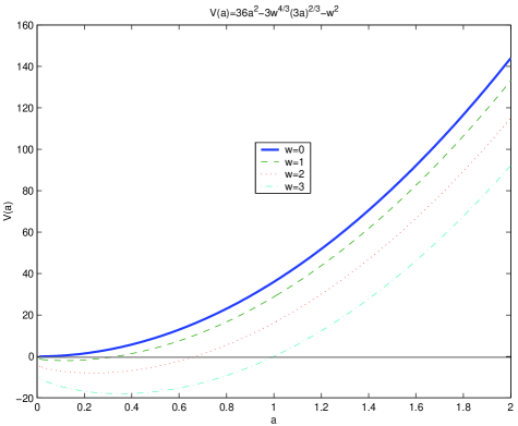
  FIG. 1.: The potential $V_{\omega}(a)$

  The classical turning point is $a=\omega/3$, and the empty brane universe can not expand classically byeond this point. The empty universe model is non-realistic, a more realistic model may include some matter fields, or at least a cosmological constant. Analysis of the cosmological constant universe can be found in [27].

• In accordance with section V, one of the necessary conditions for an Einstein solution is Eq. (96) $\int d^{3}x\,P_{A}=0$. Within our minisuperspace model, integrating the momenta (120) over the spatial manifold one gets $\int d^{3}x\,P_{A}=(P_{T},0,0,0,0)^{T}$, thus the Einstein case is associated with $\omega=0$, and the only classcal regime is $a=0$.

• The still open question is that of the boundary conditions. In particular $\Psi(a=0,T)$ and $\Psi(a\rightarrow\infty,T)$. One possibility is: $\Psi$ vanishes at the big bang ($a=0$) and $\Psi$ is bounded at $a\rightarrow\infty$. This will lead to $\omega$ quantization $\omega_{n}^{2}=8\hbar(n+1/4)$ where $n$ is a positive integer. Clearly, the Einstein case $\omega=0$ is excluded by such quatization condition.

summary

1. In the present model of Geodetic Brane Gravity, the $4$ dimensional universe floats as an extended object within a flat $m$ dimensional manifold. It can be generalized however, to include fields in the surrounding manifold (bulk), this is done by adding the bulk action integral to the action of the brane. The brane will feel those bulk fields as forces influencing its motion [22]. The bulk fields may include matter fields or the bulk gravity [19, 20, 21, 23].

2. In this paper we have derived the quadratic Hamiltonian of a brane universe. The Hamiltonian is a sum of $4$ first class constraints, while $2$ additional second class constraints are present. We used Dirac Brackets and found the algebra of first class constraints to be the familiar one from other relativistic theories (such as string, membrane or general relativity). The BRST generator turns out to be of rank $1$.

3. Geodetic brane gravity modifies general relativity, and introduces in a natural way dark matter components. Dark matter in inflationary models which accompanies ordinary matter to govern the evolution of the universe can be found in [28].

4. We have formulated the conditions for a solution to be that of general relativity, and showed that the Einstein case can be achieved only as a limiting case.

5. Canonical quantization is possible with the aid of Dirac brackets. The resulting Wheeler de-Witt equation includes operators which are not free, but are constrained by the second class constraints as operator identities.

6. The ground is ready for functional integral quantization, the BRST generator is of rank $1$, and the determinant of second class constraints has been brought to a simple form.

7. A simple application of geodetic brane gravity to cosmology is possible within the framework of a minisuperspace. Classical cosmological models appear in [25, 26]. Canonical quantization appears in [27], and the complementary functional integral quantization in [29].

8. Another significant advantage of GBG over GR is the solution to the problem of time. While a homogeneous and isotropic metric is characterized by only one dynamical variable (the scale factor of the universe), the embedding vector contains two dynamical variables (the scale factor and the bulk time). Thus, taking the embedding vector to be the canonical variables, will enhance the theory with one extra variable that may be intepreted as a time coordinate.

A Functional Derivatives

$\bullet$ Let $F[y]$ be a functional of $y(x)$ such that $\delta F=\int d^{3}xf(x)\delta y(x)$ then the functional derivative is $\displaystyle{\frac{\delta F}{\delta y(x)}\equiv f(x)}$.

The chain rule holds for functional derivatives $\displaystyle{\frac{\delta F(G[y])}{\delta y(x)}=\frac{\partial F}{\partial G}\frac{\delta G[y]}{\delta y(x)}}$

$\bullet$ The delta distribution is a scalar density of weight $1$ such that for a $3$-scalar $f(x)$

$$f(x)=\int d^{3}zf(z)\delta^{3}(x-z)$$ (A1)

The covariant derivative of the delta function $\delta^{3}_{\,|i}(x-z)$ is defined for a $3$-vector $g^{i}(x)$

$$\int d^{3}xg^{i}(x)\delta^{3}_{\,|i}(x-z)=-g^{i}_{\,|i}(z).$$ (A2)

$\bullet$ The delta function is symmetric with its two arguments

$$\delta(x-z)=\delta(z-x)~{}.$$ (A3)

The first covariant derivative of the delta function is antisymmetric with its arguments

$$\delta_{\,|i}(x-z)\equiv\nabla_{x^{i}}\delta(x-z)=-\nabla_{z^{i}}\delta(z-x)\equiv-\delta_{\,|i}(z-x)~{}.$$ (A4)

While the second covariant derivative is again symmetric.

$\bullet$ The basic functional derivatives are

$$\frac{\delta y^{A}(x)}{\delta y^{B}(z)} = \delta^{A}_{B}\delta(x-z)$$ (A5)

$$\frac{\delta y^{A}_{\,|i}(x)}{\delta y^{B}(z)} = \delta^{A}_{B}\delta_{|i}(x-z)$$ (A6)

$$\frac{\delta y^{A}_{\,|ij}(x)}{\delta y^{B}(z)} = \left(\delta^{A}_{B}-y^{A}_{\,|a}h^{ab}y_{B|b}\right)\delta_{|ij}(x-z)-y_{B|ij}y^{A}_{\,|a}h^{ak}\delta_{|k}(x-z)$$ (A7)

For a general expression $\Phi(x,y,y_{|i},y_{|ij})$ the functional derivative is

$$\frac{\delta\Phi(x)}{\delta y^{A}(z)} = \frac{\partial\Phi}{\partial y^{A}}(x)\delta(x-z)+\frac{\partial\Phi}{\partial y^{A}_{\,|i}}(x)\delta_{|i}(x-z)$$ (A8)

$$+ \frac{\partial\Phi}{\partial y^{B}_{\,|ij}}(x)\left[\left(\delta^{B}_{A}-y^{B}_{\,|b}h^{ab}y_{A|a}\right)\delta_{|ij}(x-z)-y_{A|ij}y^{B}_{\,|b}h^{bk}\delta_{|k}(x-z)\right]$$ (A9)

Another nontrivial example is the $3$-dimensional Christofel symbols $\Gamma^{i}_{kl}=h^{ij}y^{A}_{\,,j}y_{A,kl}$

$$\frac{\delta\Gamma^{i}_{kl}(x)}{\delta y^{A}(z)}=h^{ij}y_{A|kl}(x)\delta_{|j}(x-z)+h^{ij}y_{A|j}(x)\delta_{|kl}(x-z)~{}.$$ (A10)

$\bullet$ The Poisson brackets are defined in the usual way

$$\left\{F,G\right\}=\int d^{3}x\left(\frac{\delta F}{\delta y^{A}(x)}\frac{\delta G}{\delta P_{A}(x)}-\frac{\delta F}{\delta P_{A}(x)}\frac{\delta G}{\delta y^{A}(x)}\right)~{}.$$ (A11)

B Poisson Brackets of constraints

We will start with the constraints (III)

$$\phi_{0} = \frac{8\pi G}{2\sqrt{h}}\left[\left(\frac{\sqrt{h}}{8\pi G}\right)^{2}(\lambda+{\cal R}^{(3)})+P\Theta(\Psi-\lambda I)^{-1}\Theta P\right]\approx 0~{},$$ (B2)

$$\phi_{k} = y_{\,|k}\cdot P\approx 0~{},$$ (B3)

$$\phi_{4} = P_{\lambda}\approx 0~{},$$ (B4)

$$\phi_{5} = \frac{8\pi G}{2\sqrt{h}}\left[\left(\frac{\sqrt{h}}{8\pi G}\right)^{2}+P\Theta(\Psi-\lambda I)^{-2}\Theta P\right]\approx 0~{}.$$ (B5)

The PB of these constraints are listed below

$$\left\{\phi_{0}(x),\phi_{0}(z)\right\} = \left[Q^{i}(x)+Q^{i}(z)\right]\delta_{|i}(x-z)\approx 0~{}.$$ (B7)

$$\left\{\phi_{0}(x),\phi_{l}(z)\right\} = \phi_{0}(z)\delta_{|l}(x-z)-\phi_{5}\lambda_{,l}(z)\delta(x-z)\approx 0~{}.$$ (B8)

$$\left\{\phi_{0}(x),\phi_{4}(z)\right\} = \phi_{5}(z)\delta(x-z)\approx 0~{}.$$ (B9)

$$\left\{\phi_{0}(x),\phi_{5}(z)\right\} = \left[B^{i}(x)+B^{i}(z)\right]\delta_{|i}(x-z)+M(z)\delta(x-z)~{}.$$ (B10)

$$\left\{\phi_{k}(x),\phi_{l}(z)\right\} = \phi_{l}(x)\delta_{|k}(x-z)+\phi_{k}(z)\delta_{|l}(x-z)\approx 0~{}.$$ (B11)

$$\left\{\phi_{k}(x),\phi_{4}(z)\right\} = 0~{}.$$ (B12)

$$\left\{\phi_{k}(x),\phi_{5}(z)\right\} = \phi_{5}(x)\delta_{|k}(x-z)-\frac{\partial\phi_{5}}{\partial\lambda}\lambda_{|k}\delta(x-z)~{}.$$ (B13)

$$\left\{\phi_{4}(x),\phi_{4}(z)\right\} = 0~{}.$$ (B14)

$$\left\{\phi_{4}(x),\phi_{5}(z)\right\} = -\frac{\partial\phi_{5}}{\partial\lambda}\delta(x-z)~{}.$$ (B15)

$$\left\{\phi_{5}(x),\phi_{5}(z)\right\} = \left[F^{i}(x)+F^{i}(z)\right]\delta_{|i}(x-z)~{}.$$ (B16)

Where the shorthanded expressions are

$$\frac{\partial\phi_{5}}{\partial\lambda} = \frac{8\pi G}{\sqrt{h}}\left[P\Theta(\Psi-\lambda I)^{-3}\Theta P\right]$$ (B18)

$$K_{ij} = -\frac{8\pi G}{\sqrt{h}}P(\Psi-\lambda I)^{-1}y_{|ij}$$ (B19)

$$Q^{i} = h^{ij}\phi_{j}+2\left[(Kh^{ij}-K^{ij})_{|j}-\frac{8\pi G}{\sqrt{h}}h^{ij}\phi_{j}\right]\phi_{5}\approx 0$$ (B20)

$$B^{i} = \left[(Kh^{ij}-K^{ij})_{|j}-\frac{8\pi G}{\sqrt{h}}h^{ij}\phi_{j}\right]\frac{\partial\phi_{5}}{\partial\lambda}+\left[\frac{\partial(Kh^{ij}-K^{ij})}{\partial\lambda}\right]_{|j}\phi_{5}$$ (B21)

$$\approx \left[(Kh^{ij}-K^{ij})_{|j}\right]\frac{\partial\phi_{5}}{\partial\lambda}$$ (B22)

$$M \approx \frac{\sqrt{h}}{8\pi G}\left[\lambda\frac{\partial K}{\partial\lambda}-K+(R_{ij}-2K_{il}K_{j}^{l})\frac{\partial}{\partial\lambda}(Kh^{ij}-K^{ij})\right]$$ (B25)

$$+(Kh^{ij}-K^{ij})_{|j}\left[\left(\frac{\partial\phi_{5}}{\partial\lambda}\right)_{|i}-2\frac{8\pi G}{\sqrt{h}}[P(\Psi-\lambda I)^{-1}]_{|i}(\Psi-\lambda I)^{-2}P\right]$$

$$-\frac{8\pi G}{\sqrt{h}}P(\Psi-\lambda I)^{-1}[(\Psi-\lambda I)^{-1}P]_{|ij}\frac{\partial}{\partial\lambda}(Kh^{ij}-K^{ij})$$

$$F^{i} \approx \frac{1}{3}\frac{\partial^{2}\phi_{5}}{\partial\lambda^{2}}\left(Kh^{ij}-K^{ij}\right)_{|j}$$ (B28)

$$-\left(\frac{\partial\phi_{5}}{\partial\lambda}\right)^{2}\left[\left(\frac{\partial\phi_{5}}{\partial\lambda}\right)^{-1}\frac{\partial}{\partial\lambda}(Kh^{ij}-K^{ij})\right]_{|j}$$

$$-2\frac{8\pi G}{\sqrt{h}}P(\Psi-\lambda I)^{-2}\left[(\Psi-\lambda I)^{-1}P\right]_{|j}\frac{\partial}{\partial\lambda}(Kh^{ij}-K^{ij})$$

C Matter Hamiltonians

Consider here a few simple matter Lagrangians and Hamiltonians,

$\bullet$ For a cosmological constant ,

$${\cal L}_{matter} = -\sqrt{-g}2\Lambda~{},$$ (C2)

$$T^{\alpha\beta} = -2\Lambda g^{\alpha\beta}~{}.$$ (C3)

The corresponding energy/momentum projections are

$$T_{nn} = 2\Lambda~{},$$ (C5)

$$T_{ni} = 0~{}.$$ (C6)

The Hamiltonian is simply

$${\cal H}_{matter}=-{\cal L}_{matter}=N\sqrt{h}2\Lambda=N\sqrt{h}T_{nn}~{}.$$ (C7)

$\bullet$ For a scalar field $\Phi(x)$,

$${\cal L}_{matter} = -\sqrt{-g}\left(\frac{1}{2}g^{\mu\nu}\partial_{\mu}\Phi\partial_{\nu}\Phi+V(\Phi)\right)~{},$$ (C9)

$$T^{\alpha\beta} = \left(g^{\alpha\mu}g^{\beta\nu}-\frac{1}{2}g^{\alpha\beta}g^{\mu\nu}\right)\partial_{\mu}\Phi\partial_{\nu}\Phi-g^{\alpha\beta}V(\Phi)~{}.$$ (C10)

The momentum $\Pi$ conjugate to $\Phi$ is given by

$$\Pi=\frac{\delta{\cal L}}{\delta\dot{\Phi}}=\sqrt{h}\frac{1}{N}(\dot{\Phi}-N^{i}\Phi_{,i})~{},$$ (C11)

and the corresponding energy/momentum projections are

$$T_{nn} = \frac{1}{2}\left(\frac{1}{h}\Pi^{2}+h^{ij}\Phi_{,i}\Phi_{,j}\right)+V~{},$$ (C13)

$$T_{ni} = \frac{1}{\sqrt{h}}\Pi\Phi_{,i}~{}.$$ (C14)

The matter Hamiltonian is

$${\cal H}_{matter}=N\sqrt{h}(\frac{1}{2h}\Pi^{2}+\frac{1}{2}h^{ij}\Phi_{,i}\Phi_{,j}+V)+N^{i}\Pi\Phi_{,i}=N\sqrt{h}T_{nn}+N^{i}\sqrt{h}T_{ni}~{}.$$ (C15)

$\bullet$ For a vector field $A_{\mu}(x)$,

$${\cal L}_{matter} = -\frac{1}{16\pi}\sqrt{-g}g^{\mu\lambda}g^{\nu\sigma}F_{\mu\nu}F_{\lambda\sigma}~{},$$ (C17)

$$T^{\alpha\beta} = \frac{1}{4\pi}\left(g^{\alpha\mu}g^{\beta\nu}-\frac{1}{4}g^{\alpha\beta}g^{\mu\nu}\right)g^{\lambda\sigma}F_{\mu\lambda}F_{\nu\sigma}~{}.$$ (C18)

The momentum $\Pi^{\mu}$ conjugate to $A_{\mu}$ is given by

$$\Pi^{0} = 0~{},$$ (C20)

$$\Pi^{i} = \frac{\sqrt{h}}{4\pi N}h^{ij}\left(\dot{A}_{j}-A_{0,j}-N^{k}F_{kj}~{},\right)$$ (C21)

and the corresponding energy/momentum projections are

$$T_{nn} = \frac{2\pi}{h}h^{ij}\Pi_{i}\Pi_{j}+\frac{1}{16\pi}h^{ij}h^{kl}F_{ik}F_{jl}~{},$$ (C23)

$$T_{ni} = \frac{1}{\sqrt{h}}h^{kl}\Pi_{k}F_{il}~{}.$$ (C24)

The Hamiltonian is

$${\cal H}=N\sqrt{h}(\frac{2\pi}{h}h^{ij}\Pi_{i}\Pi_{j}+\frac{1}{16\pi}h^{ij}h^{kl}F_{ik}F_{jl})+N^{i}\Pi^{j}F_{ij}-A_{0}\Pi^{i}_{\,,i}=N\sqrt{h}T_{nn}+N^{i}\sqrt{h}T_{ni}-A_{0}\Pi^{i}_{\,,i}~{}.$$ (C25)

In this case the Hamiltonian picks up another Lagrange multiplier $A_{0}$, and an additional constraint

$$-\Pi^{i}_{\,,i}=\frac{1}{4\pi}\sqrt{-g}F^{0\nu}_{\hskip 5.0pt;\nu}=0~{}.$$ (C26)

D The center of mass and relative coordinates

We will try to make a canonical transformation to the new system. We will use a global pair ${\bf Y}^{A}(t),{\bf P}_{A}(t)$ to describe the total momentum and its conjugate coordinate. And, as relative coordinates we will use the directional derivatives $z^{A}_{\,i}(x)=y^{A}_{\,,i}(x)$ of the field $y^{A}(x)$. (This is the analog to a discrete system, where the relative coordinates are differences between the coordinates of the various particles involved).

The variation of the Action with respect to $y^{A}_{\,,i}(x)$ is going to be very similar to the variation with respect to $h_{ij}$, and therefore will resemble Einstein’s equations. The new set of canonical ’coordinates $+$ fields’ ${\bf Y}^{A},{\bf P}_{A},z^{A}_{\,i}(x),\pi_{A}^{\,i}(x)$, must obey the canonical PB

$$\left\{{\bf Y}^{A},{\bf P}_{B}\right\} = \delta^{A}_{B}~{},$$ (D2)

$$\left\{{\bf Y}^{A},\pi_{B}^{\,i}(x)\right\} = 0~{},$$ (D3)

$$\left\{z^{A}_{\,i}(x),{\bf P}_{B}\right\} = 0~{},$$ (D4)

$$\left\{z^{A}_{\,i}(x),\pi_{B}^{\,j}(\bar{x})\right\} = \delta^{A}_{B}\delta_{i}^{\,j}\delta(x-\bar{x})~{}.$$ (D5)

We will write the transformation from the old set of fields to the new set as

$${\bf Y}^{A}(t) = \int d^{3}x\,f(x)y^{A}(t,x)$$ (D7)

$${\bf P}_{A}(t) = \int d^{3}x\,P_{A}(t,x)$$ (D8)

$$z^{A}_{\,i}(t,x) = y^{A}_{\,,i}(t,x)$$ (D9)

$$\pi_{A}^{\,i}(t,x) = \int d^{3}\bar{x}\,P_{A}(t,\bar{x})J^{i}(x,\bar{x})$$ (D10)

While the inverse transformation is

$$y^{A}(t,x) = {\bf Y}^{A}(t)+\int d^{3}\bar{x}\,z^{A}_{\,i}(t,\bar{x})J^{i}(\bar{x},x)$$ (D12)

$$P_{A}(t,x) = {\bf P}_{A}(t)f(x)-\pi^{i}_{A\;,i}(t,x)$$ (D13)

The functions $f(x),J^{i}(x,\bar{x})$ are distributions over the $V_{3}$ manifold, they do not depend on the canonical fields, and in particular are independent of the $3$-metric. The solution to Eq.(D) put some restrictions on $f(x),J^{i}(x,\bar{x})$, and they must fulfill the following relations

$$\int d^{3}x\,f(x) = 1~{},$$ (D15)

$$\int d^{3}\bar{x}\,f(\bar{x})J^{i}(x,\bar{x}) = 0~{},$$ (D16)

$$\frac{\partial J^{i}(x,\bar{x})}{\partial\bar{x}^{j}} = \delta^{i}_{j}\delta(x-\bar{x})~{},$$ (D17)

$$\frac{\partial J^{i}(x,\bar{x})}{\partial x^{i}} = f(x)-\delta(x-\bar{x})~{}.$$ (D18)

We assume one can find such distributions and we move on to the dynamics. We will start with the Hilbert action (1) and do the variation with respect to the new variables

$$\delta S = \frac{-1}{16\pi G}\int d^{4}x\,\sqrt{-g}(G^{\mu\nu}-8\pi GT^{\mu\nu})\delta g_{\mu\nu}$$ (D19)

$$= \frac{-2}{16\pi G}\int d^{4}x\,\sqrt{-g}(G^{\mu\nu}-8\pi GT^{\mu\nu})y_{A,\mu}\delta y^{A}_{\,,\nu}$$ (D20)

$$= \frac{2}{16\pi G}\int d^{4}x\,\left\{\left[\sqrt{-g}(G^{\mu 0}-8\pi GT^{\mu 0})y_{A,\mu}\right]_{,0}\left[\delta{\bf Y}^{A}+\int d^{3}\bar{x}\,\delta z^{A}_{\,i}(\bar{x})J^{i}(\bar{x},x)\right]\right.$$ (D21)

$$- \frac{2}{16\pi G}\int d^{4}x\,\sqrt{-g}(G^{\mu i}-8\pi GT^{\mu i})y_{A,\mu}\delta z^{A}_{\,i}(x)~{},$$ (D22)

The variation with respect to ${\bf Y}^{A}$ will lead to the conservation of the total momentum

$$\frac{-2}{16\pi G}\int d^{3}x\,\left[\sqrt{-g}(G^{\mu 0}-8\pi GT^{\mu 0})y_{A,\mu}\right]=\mu_{A}=\text{const.}$$ (D23)

The variation with respect to $z^{A}_{\,i}(x)$ will lead to an equation similar to Einstein’s equations, but, the right hand side does not vanish

$$\sqrt{-g}\,y_{A,\alpha}[G^{\alpha i}-8\pi GT^{\alpha i}](x)=\int d^{3}\bar{x}J^{i}(x,\bar{x})\left[\sqrt{-g}(G^{\alpha 0}-8\pi GT^{\alpha 0})y_{A,\alpha}(\bar{x})\right]_{,0}~{}.$$ (D24)

Multiply Eq.(D24) by $\frac{1}{\sqrt{-g}}g^{\mu\nu}y^{A}_{\,,\nu}$ to get

$$G^{\mu i}-8\pi GT^{\mu i}(x)=D^{\mu i}(x)=\frac{1}{\sqrt{-g}}g^{\mu\nu}y^{A}_{\,,\nu}(x)\int d^{3}\bar{x}J^{i}(x,\bar{x})\left[\sqrt{-g}(G^{\alpha 0}-8\pi GT^{\alpha 0})y_{A,\alpha}(\bar{x})\right]_{,0}~{}.$$ (D25)

An Einstein physicist will interpret Eq.(D25) as if there is some additional matter in the universe, and may call it dark matter.

It is easy to reveal Eq.(3) if one takes the derivative of Eq.(D24) with respect to $x^{i}$ and use (D18).

E Determinant of second class constraints PB

We would like to calculate the determinant of $C_{mn}(x,z)$ (74). First we will find the eigenvalues of $C$. Take $v(x)$ to be a two components scalar function

$$v(x)=\left(\begin{array}[]{c}g(x)\\ f(x)\end{array}\right)~{}.$$ (E1)

The eigenvalue equation of $C$ is

$$\int d^{3}z\,C(x,z)v(z)=\alpha v(x)~{}.$$ (E2)

Inserting Eq.(74) into Eq.(E2) one can see that the components of $v(x)$ are proportional, and must obey a differential equation

$$g=-\frac{1}{\alpha}\frac{\partial\phi_{5}}{\partial\lambda}f~{},$$ (E4)

$$2F^{i}f_{|i}+F^{i}_{|i}f-\frac{1}{\alpha}\left(\frac{\partial\phi_{5}}{\partial\lambda}\right)^{2}f=\alpha f~{}.$$ (E5)

Multiplying (E5) by $f$ one gets

$$\left(F^{i}f^{2}\right)_{|i}=\left[\alpha+\frac{1}{\alpha}\left(\frac{\partial\phi_{5}}{\partial\lambda}\right)^{2}\right]f^{2}~{}.$$ (E6)

Eigenvalues of a differential operator are determined by the boundary conditions. Our boundary conditions are actually the fact that the $3$-manifold has no boundary. Thus integrating Eq.(E6) over $V_{3}$ gives us

$$\int d^{3}x\left[\alpha+\frac{1}{\alpha}\left(\frac{\partial\phi_{5}}{\partial\lambda}\right)^{2}\right]f^{2}(x)=0~{}.$$ (E7)

Arranging Eq.(E7) one gets

$$\alpha^{2}=-\frac{\int d^{3}x\left(\frac{\partial\phi_{5}}{\partial\lambda}\right)^{2}f^{2}(x)}{\int d^{3}xf^{2}(x)}~{}.$$ (E8)

• $C_{mn}(x,z)$ is a PB matrix and therefore antihermitian, this causes the eigenvalues of $C$ to be purely imaginary.

• One can see that the eigenvalues of $C$ are affected only by the off diagonal terms $\frac{\partial\phi_{5}}{\partial\lambda}$, not by $F^{i}$.

The structure of $\alpha^{2}$ is very simple. Define the probability density

$$\bar{f}(x)\equiv\frac{f^{2}(x)}{\int d^{3}xf^{2}(x)}~{},$$ (E9)

one sees that any eigenvalue of $C$ is simply the expectation value of $\left(\frac{\partial\phi_{5}}{\partial\lambda}\right)^{2}$ with respect to some probability distribution $\bar{f}$

$$\alpha^{2}_{\bar{f}}=-\left\langle\left(\frac{\partial\phi_{5}}{\partial\lambda}\right)^{2}\right\rangle_{\bar{f}}~{}.$$ (E10)

For each $\bar{f}$ one finds $2$ complex conjugate purely imaginary eigenvalues. The determinant of $C$ is therefore the multiplication of all eigenvalues

$$\det C=\prod_{\bar{f}}\left\langle\left(\frac{\partial\phi_{5}}{\partial\lambda}\right)^{2}\right\rangle_{\bar{f}}$$ (E11)

The probability density over a compact manifold can be parameterized by the appropriate harmonics, and the product is countable. See for example [30, 31] for the compact $S_{3}$ harmonics.

REFERENCES

- [1] T. Regge and C. Teitelboim, in Proc. Marcel Grossman, p.77 (Trieste, 1975).
- [2] S. Deser, F.A.E. Pirani, and D.C. Robinson, Phys. Rev. D14, 3301 (1976).
-
[3]
V. Tapia, Class. Quan. Grav. 6, L49 (1989);
M. Pavsic, Phys. Lett. A107, 66 (1985);
C. Maia, Class. Quan. Grav. 6, 173 (1989);
I. A. Bandos, Mod. Phys. Lett. A12, 799 (1997). -
[4]
E. Cartan, Ann. Soc. Pol. Math. 6,
1 (1928);
M. Janet, Ann. Soc. Pol. Math. 5, 38 (1926);
A. Friedman, Rev. Mod. Phys. 37, 201 (1965). - [5] J Rosen, Rev. Mod. Phys. 37, 204 (1965).
-
[6]
J. W. York, pp. 246-254 in Between Quantum and
Cosmos, eds. W. H. Zurek and W. A. Miller (Princeton Univ. Press,
Princeton N.J., 1988);
T. Regge and C. Teitelboim, Ann. Phys. 88 (1974) 286;
G. W. Gibbons and S. W. Hawking, Phys. Rev. D15, 2752 (1977). -
[7]
P.A.M. Dirac, Lectures on quantum mechanics,
(Belfer Graduate School of Science
Yeshiva University, New York, 1964);
K. Sundermeyer, Constrained Dynamics with Application to Yang-Mills Theory, General Relativity, Ckassicak Spin, Dual string Model, (Springer, Berlin, 1982);
A. Hanson, T. Regge and C. Teitelboim, Constrained Hamiltonian Systems, (Academia Nazionale dei Lincei, Rome, 1976). - [8] R. Arnowitt, S. Deser and C. Misner, in Gravitation: An Introduction to Current Research, ed. L. Witten (New York, Wiley, 1962).
- [9] C.W. Misner, K. Thorne and J.A. Wheeler, Gravitation, (W.H. Freeman, San-Francisco, 1973).
- [10] S.W. Hawking and G.F.R. Ellis, The Large Scale Structure of Spacetime, (Cambridge Univ. Press, Cambridge, England, 1973).
- [11] D. Kramer, H. Stephani, E. Herlt, and M. MacCallum, Exact Solutions of Einstein’s Field Equations, (Cambridge Univ. Press, Cambridge, 1980), p.354-374;
-
[12]
J.B. Hartle and S.W. Hawking, Phys.
Rev. D 28, 2960 (1983);
J.J. Halliwell and J.B. Hartle, Phys. Rev. D 43, 1170 (1991);
J.J. Halliwell, Phys. Rev. D 38, 2468 (1988). - [13] J.J. Halliwell, Phys. Rev. D 38, 2468 (1988).
- [14] R. P. Feynman and Hibbs, Quantum Mechanics and Path Integrals, (McGraw-Hill, New york) 1965.
-
[15]
E.S. Fradkin and G.A. Vilkovisky, Phys. Lett.
55B, 224 (1975);
I.A. Batalin and G.A. Vilkovisky, Phys. Lett. 69B, 309 (1977);
L.D. Faddeev and V.N. Popov, Phys. Lett. 25B, 29 (1967). - [16] E.S. Fradkin and T.E. Fradkina, Phys. Lett. 72B, 343 (1978).
- [17] C. Becchi, A. Rouet and R. Stora, Ann. Phys. 98, 287 (1976).
- [18] P. Senjanovic, Ann. Phys. 100,227 (1975).
-
[19]
L. Randall and R. Sundrum, Phys. Rev. Lett. 83,
3370 (1999);
L. Randall and R. Sundrum, Phys. Rev. Lett. 83, 4690 (1999). -
[20]
N. Arkani-Hamed, S. Dimopoulus and G. Dvali,
Phys. Lett. B 429, 263 (1998);
I. Antoniadis, N. Arkani-Hamed, S. Dimopoulus and G. Dvali, Phys. Lett. B 436, 257 (1998);
G. Dvali, G. Gabadadze and M. Porrati, Phys. Lett. B 484, 112 (2000);
R. Dick, hep-th/0105320. - [21] D. Ida, JHEP 0009, 014 (2000).
-
[22]
B. Carter, j-P. Uzan, R.A. Battye and A. Mennim,
Class. Quan. Grav. 18, 4871 (2001);
R.A. Battye and B. Carter hep-th/0101061;
B. Carter gr-qc/0012036. - [23] R. Cordero and A. Vilenkin, hep-th/0107175.
- [24] A. Davidson and D. Karasik, Mod. Phys. Lett. A13, 2187 (1998).
- [25] A. Davidson, Class. Quant. Grav. 16, 653 (1999).
- [26] A. Davidson, D. Karasik, and Y. Lederer, hep-th/0112061.
- [27] A. Davidson, D. Karasik, and Y. Lederer, Class. Quan. Grav. 16, 1349 (1999).
- [28] A. Davidson, D. Karasik, and Y. Lederer, gr-qc/0111107.
- [29] A. Davidson, D. Karasik, and Y. Lederer, (in preparation).
- [30] J.J. Haliwell and S.W. Hawking, Phys. Rev. D31, 1777 (1985).
- [31] U. H. Gerlach and U. K. Sengupta, Phys. Rev. D18, 1773 (1978).