Asymptotic Behavior of a Class of Expanding Gowdy Spacetimes

Abstract

A systematic asymptotic expansion is developed for the gravitational wave degrees of freedom of a class of expanding, vacuum Gowdy cosmological spacetimes. In the wave map description of these models, the evolution of the gravitational wave amplitudes defines an orbit in the target space. The circumference of this orbit decays to zero indicating that the asymptotic spacetime is spatially homogeneous. A prescription is given to identify the asymptotic cosmological model for the gravitational wave degrees of freedom using the asymptotic point in the target space. The remaining metric function of the asymptotic cosmological model, found by solving the constraints, is determined by an effective energy of the gravitational waves rather than from the asymptotic point in the target space.

I Introduction

Current understanding of cosmology relies heavily on the assumption that the large-scale dynamics of the observable universe may be described by an averaged matter distribution evolving in a spatially homogeneous (and isotropic) background. Yet it is clear that the universe is characterized by spatial inhomogeneities that may be large and might be dynamically relevant. Some studies have been made to provide a rigorous basis for the validity of the standard cosmological approach but the question is not settled Kasai (1993); Tomita and Deruelle (1994); Deruelle and Langlois (1995); Carfora and Piotrkowska (1995); Futamase (1996); Stoeger et al. ; Buchert .

The Gowdy cosmological spacetimes Gowdy (1971); Berger (1974) have proven to be valuable theoretical laboratories to explore the behavior of spatially inhomogeneous cosmologies. For example, polarized and generic Gowdy models on $T^{3}\times R$ provided the first detailed demonstration of the Belinskii et al (BKL) Belinskii et al. (1971) claim that, in the collapse direction, each spatial point of a generic cosmological spacetime evolves toward the singularity as a separate universe Isenberg and Moncrief (1990); Berger and Moncrief (1993); Berger and Garfinkle (1998).

Polarized Gowdy models have also been studied in the expanding direction, both for $T^{3}$ Berger (1974) and $R^{3}$ Centrella and Matzner (1982) spatial topology, where it was argued that the asymptotic behavior could be understood as a stiff fluid of gravitational waves propagating in a spatially homogeneous background spacetime. Related numerical studies of fluids in plane symmetric expanding cosmologies have also been discussed Anninos (1998); Anninos and McKinney (1999). In this paper, we will argue that this type of asymptotic picture, previously obtained for the polarized case, persists for a large class of generic Gowdy models. We shall also demonstrate how the background cosmology may be extracted from a numerical simulation of these spacetimes.

Ringström has recently shown Ringström that expanding Gowdy spacetimes fall into two classes with qualitatively different behaviors. Only one of these classes is considered here.

II Gowdy model on $T^{3}\times R$

The vacuum Gowdy cosmology on $T^{3}\times R$ is described by the metric Gowdy (1971); Berger and Moncrief (1993); Berger and Garfinkle (1998)

$$ds^{2}=e^{\lambda/2}\,t^{-1/2}\,(-\,dt^{2}\,+\,d\theta^{2})\,+\,t\,\left[e^{P}\,(dx\,+\,Q\,dy)^{2}\,+\,e^{-P}\,dy^{2}\right]$$ (1)

where $0<t<\infty$, $\theta\,\in\,[0,2\pi]$, $\{x,y\}\,\in\,T^{2}$, and the gravitational wave amplitudes $P$, $Q$ and the background variable $\lambda$ depend only on $\theta$ and $t$. If one assumes that $P$ and $Q$ are small, it is easy to see that $P$ is related to the amplitude of the $+$ polarization and $Q$ to the $\times$ polarization of gravitational waves. (See Berger (1974); Berger and Moncrief (1993) for discussion of the interpretation of these variables.) Einstein’s equations become (with the notation that $z,_{t}=\partial z/\partial t$)

$$P,_{tt}\,+\,{1\over t}P,_{t}\,-\,P,_{\theta\theta}\,+\,e^{2P}\left(Q,_{\theta}^{2}\,-\,Q,_{t}^{2}\right)=0$$ (2)

and

$$Q,_{tt}\,+\,{1\over t}Q,_{t}\,-\,Q,_{\theta\theta}\,+\,2\,P,_{t}\,Q,_{t}\,-\,2\,P,_{\theta}\,Q,_{\theta}=0$$ (3)

for the wave amplitudes and

$$\lambda,_{t}\,-\,t\,\left(P,_{t}^{2}\,+\,e^{2P}Q,_{t}^{2}\,+\,P,_{\theta}^{2}\,+\,e^{2P}Q,_{\theta}^{2}\right)=0$$ (4)

and

$$\lambda,_{\theta}\,-\,2\,t\,(P,_{t}P,_{\theta}\,+\,e^{2P}Q,_{t}Q,_{\theta})=0$$ (5)

for the background . Note that Eqs. (4) and (5) are respectively the Hamiltonian and momentum constraints and that $\lambda$ may be constructed after the wave equations (2) and (3) are solved for $P$ and $Q$. The periodic boundary conditions imposed on the metric by $T^{3}$ spatial topology require Berger (1974)

$$\oint\,\lambda,_{\theta}\,d\theta=0$$ (6)

which may be understood as a restriction on $P$ and $Q$ through Eq. (5). This condition must be imposed on the initial data and is preserved by the evolution.

Numerical simulation is straightforward since the spiky features which are prominent in collapse Berger and Moncrief (1993); Berger and Garfinkle (1998) do not develop in the expansion direction. However, in contrast to the dominance of local behavior in collapsing models, the global behavior is dynamically important so that, at any $t$, the spatial waveforms must be obtained accurately.

If we specialize to the case that $P$, $Q$, and $\lambda$ depend on $t$ only, Einstein’s equations reduce to the spatially homogeneous equations (where overdot $=d/dt$) Berger and Moncrief (1993)

$$\ddot{P}\,+\,{1\over t}\dot{P}\,-\,e^{2P}\dot{Q}^{2}=0,$$ (7)

$$\ddot{Q}\,+\,{1\over t}\dot{Q}\,+\,2\,\dot{P}\dot{Q}=0,$$ (8)

and

$$\dot{\lambda}\,-\,t\,\left(\dot{P}^{2}\,+\,e^{2P}\dot{Q}^{2}\right)=0$$ (9)

with the known spatially homogeneous solution Berger et al. (1998)

$$P=\ln|\mu|\,+\,v\ln\left({t\over{t_{0}}}\right)\,+\,\ln\left[1\,+\,\left({t\over{t_{0}}}\right)^{-2v}\right],$$ (10)

$$Q=\xi\,+\,{1\over{\mu\left[1\,+\,\left({t\over{t_{0}}}\right)^{-2v}\right]}},$$ (11)

and

$$\lambda=\lambda_{0}+v^{2}\,\ln\,t$$ (12)

where $\mu$, $\xi$, $v$, $t_{0}$, and $\lambda_{0}$ are constants. For convenience, consider only the case $v>0$ as $t\to\infty$. The metric becomes (where some constants have been absorbed and with $Q\to c$ as $t\to\infty$)

$$ds^{2}=t^{(v^{2}-1)/2}(-dt^{2}\,+\,d\theta^{2})\,+\,t^{1+v}(dx\,+\,cdy)^{2}\,+\,t^{1-v}dy^{2}.$$ (13)

The contribution due to $Q$ (i.e. the constant $c$) rotates the coordinate axes with respect to two of the Killing directions. In terms of comoving proper time, $T$, defined by

$$T=t^{(v^{2}+3)/4}$$ (14)

(where again some constants have been absorbed), the metric (13) becomes

$$ds^{2}=-dT^{2}\,+\,T^{2(v^{2}-1)/(v^{2}+3)}d\theta^{2}\,+\,T^{4(1+v)/(v^{2}+3)}(dx\,+\,cdy)^{2}\,+\,T^{4(1-v)/(v^{2}+3)}dy^{2}.$$ (15)

The exponents of the scale factors $T^{k_{i}}$ are clearly seen to satisfy the Kasner relations $\textstyle\sum_{k=1}^{3}k_{i}=1=\textstyle\sum_{k=1}^{3}k_{i}^{2}$. We shall see later that the presence of spatial inhomogeneities (gravitational waves) will modify this Kasner background spacetime.

As is well-known (see e.g. Berger and Moncrief (1993)), the Gowdy wave equations (2) and (3) may be regarded as wave maps with the target space described by the metric

$$d{\mathcal{S}}^{2}=dP^{2}\,+\,e^{2P}dQ^{2}.$$ (16)

A spatially homogeneous solution $\{P,Q\}(t)$ is represented by a point in the target space while a spatially inhomogeneous solution $\{P,Q\}(t,\theta)$ yields a closed curve in the target space. If, asymptotically as $t\to\infty$, a spatially inhomogeneous solution approaches a spatially homogeneous one, the circumference of the curve will asymptotically approach zero and the asymptotic point thus obtained will identify the asymptotic spatially homogeneous solution. The symmetries of the target space yield three constants of the motion for the spatially homogeneous equations (7), (8):

$$\tilde{A}=\pi_{Q}\,Q\,-\,\pi_{P},$$ (17)

$$\tilde{B}=\pi_{Q},$$ (18)

$$\tilde{C}=\pi_{Q}\,\left(e^{-2P}\,-\,Q^{2}\right)\,+\,2Q\,\pi_{P},$$ (19)

where $\pi_{P}=-tP,_{t}$ and $\pi_{Q}=-t\,e^{2P}Q,_{t}$ are the momenta canonically conjugate to $P$ and $Q$. These constants may be related to the constants of the spatially homogeneous solution (10) and (11) through

$$v=\sqrt{\tilde{A}^{2}\,+\,\tilde{B}\tilde{C}}\ ,\quad\mu=-{{\tilde{B}}\over{2v}}\ ,\quad\xi=-{{\tilde{A}\,+\,v}\over{2v\mu}}\ .$$ (20)

Although $\tilde{A}$, $\tilde{B}$, and $\tilde{C}$ are not constants of the motion for the wave equations (2) and (3), their spatial averages $A$, $B$, and $C$ are constants of the motion. The dynamics of spatially inhomogeneous Gowdy models falls into two classes depending on the sign of $A^{2}+BC$ Ringström . Here we consider only $A^{2}+BC>0$, the only case allowed for solutions to the spatially homogeneous equations (7) and (8) and the case assumed in the definition of $v$ in Eq. (20). We shall show later that knowledge of $A$, $B$, and $C$ allows the asymptotic point in the target space associated with the asymptotic spatially homogeneous solution to be identified.

III Perturbation Analysis

To understand the asymptotic ($t\to\infty$) behavior of this class of expanding Gowdy models and the dynamical role of the gravitational waves assume that $P$ and $Q$ may be expressed as asymptotic expansions

$$P=p_{0}(t)\,+\,\varepsilon\,p_{1}(\theta,t)\,+\,\varepsilon^{2}\,p_{2}(\theta,t)\,+\,\ldots,$$ (21)

$$Q=\varepsilon\,q_{1}(\theta,t)\,+\,\varepsilon^{2}\,q_{2}(\theta,t)\,+\,\ldots$$ (22)

where $\varepsilon$ is a small parameter and the order $\varepsilon^{0}$ term in $Q$ is set equal to zero.. These asymptotic forms are substituted into Eqs. (2) and (3) and terms collected according to their order in powers of $\varepsilon$.

In the development of this perturbation series, it is convenient to insist as we have done here that the order $\varepsilon^{0}$ solution be polarized—i.e., we require $q_{0}(t)=0=\dot{q}_{0}(t)$. Then the order $\varepsilon^{0}$ equations are just the polarized version of Eqs. (7) and (8) which reduce to

$$\ddot{p}_{0}\,+\,{1\over t}\dot{p}_{0}=0$$ (23)

with the general solution

$$p_{0}=\alpha\,+\,v\ln t$$ (24)

where $\alpha$ and $v$ are constants. This restriction on the order $\varepsilon^{0}$ solution is not a loss of generality within this class of solutions since any solution to Eqs. (7) and (8) with $A^{2}+BC>0$ may be obtained from a polarized solution through an $SL(2,R)$ transformation . (See, for example, Berger and Moncreif (2000).)

To order $\varepsilon^{1}$, Eqs. (2) and (3) become

$$p_{1},_{tt}\,+\,{1\over t}\,p_{1},_{t}\,-\,p_{1},_{\theta\theta}\equiv{\mathcal{L}}_{P}\,p_{1}=0,$$ (25)

$$q_{1},_{tt}\,+\,\left({1\over t}\,+\,{{2v}\over t}\right)q_{1},_{t}\,-\,q_{1},_{\theta\theta}\equiv{\mathcal{L}}_{Q}\,q_{1}=0.$$ (26)

(Note that the second term within the parenthesis in Eq. (26) is $2\dot{p}_{0}$.) The general solutions to these linear equations are (with arbitrary constants chosen to eliminate the spatially homogeneous modes of $p_{1}$ and $q_{1}$)

$$p_{1}=\sum_{n=1}^{N}\,b_{n}\,{\mathcal{Z}}_{0}(nt)\,\cos(n\theta+\phi_{n}),$$ (27)

$$q_{1}=t^{-v}\,\sum_{n=1}^{N}\,d_{n}\,{\mathcal{Z}}_{\pm v}(nt)\,\cos(n\theta+\psi_{n})$$ (28)

where $n=1,\,2,\,\ldots,N$, $a_{n}$, $b_{n}$, $\phi_{n}$, and $\psi_{n}$ are constants with ${\mathcal{Z}}_{\nu}(x)$ any Bessel function of order $\nu$ . We note that the regular and irregular Bessel functions, $J_{\nu}(z)$ and $Y_{\nu}(z)$ respectively, have the following large-argument asymptotic expansions Abramowitz and Stegun (1965):

$$J_{\nu}(z)=\sqrt{{2\over{\pi z}}}\left[\cos(z-{\pi\over 2}\nu-{\pi\over 4})-{{4\nu^{2}-1}\over{8z}}\sin(z-{\pi\over 2}\nu-{\pi\over 4})+\ldots\right]\,,$$ (29)

$$Y_{\nu}(z)=\sqrt{{2\over{\pi z}}}\left[\sin(z-{\pi\over 2}\nu-{\pi\over 4})+{{4\nu^{2}-1}\over{8z}}\cos(z-{\pi\over 2}\nu-{\pi\over 4})+\ldots\right]\,,$$ (30)

$$J^{\prime}_{\nu}(z)=\sqrt{{2\over{\pi z}}}\left[-\sin(z-{\pi\over 2}\nu-{\pi\over 4})-{{4\nu^{2}+3}\over{8z}}\cos(z-{\pi\over 2}\nu-{\pi\over 4})+\ldots\right]\,,$$ (31)

$$Y^{\prime}_{\nu}(z)=\sqrt{{2\over{\pi z}}}\left[\cos(z-{\pi\over 2}\nu-{\pi\over 4})-{{4\nu^{2}+3}\over{8z}}\sin(z-{\pi\over 2}\nu-{\pi\over 4})+\ldots\right]\,,$$ (32)

where a prime indicates the derivative with respect to the argument. These asymptotic forms for the Bessel functions indicate that (1) an arbitrary superposition of Bessel functions of order $\nu$ and argument $nt$ can be represented asymptotically as

$${\mathcal{Z}}_{\nu}(nt)\to\xi_{n}\sqrt{{2}\over{\pi nt}}\cos(nt+\varphi_{n})$$ (33)

where the constant $\xi_{n}$ includes any normalization and $\varphi_{n}$ is an arbitrary phase; (2) as $t\to\infty$, the leading terms in Eqs. (27) and (28) of the form ${\mathcal{Z}}_{\nu}(nt)\cos(n\theta+\delta_{n})$ have the property that the leading terms of the derivatives with respect to $t$ (or, trivially, $\theta$) decay as $1/\sqrt{t}$—i.e., to leading order in inverse powers of $t$, the derivative acts only on the trigonometric functions.

To order $\varepsilon^{2}$, Eqs. (2) and (3) become

$${\mathcal{L}}_{P}\,p_{2}=e^{2p_{0}}\left(q_{1},_{t}^{2}\,-\,q_{1},_{\theta}^{2}\right),$$ (34)

$${\mathcal{L}}_{Q}\,q_{2}=2\,p_{1},_{\theta}\,q_{1},_{\theta}\,-\,2\,p_{1},_{t}\,q_{1},_{t}.$$ (35)

The order $\varepsilon^{2}$ solutions may be expressed as Fourier series (chosen, for convenience, to be the sum of a finite number of terms),

$$p_{2}(\theta,t)=p_{2}^{(0)}(t)\,+\,\sum_{k=1}^{N}p_{2}^{(k)}(t)\cos(k\theta+\phi_{k}),$$ (36)

$$q_{2}(\theta,t)=q_{2}^{(0)}(t)\,+\,\sum_{k=1}^{N}q_{2}^{(k)}(t)\cos(k\theta+\psi_{k}).$$ (37)

The spatially homogeneous modes $p_{2}^{(0)}$, $q_{2}^{(0)}$ could, in principle, seriously modify the background spacetime if they are not small compared to $p_{0}$ (and, in general, $q_{0}$). Integration over the circle of Eqs. (34) and (35) yields

$$\ddot{p}_{2}^{(0)}\,+\,{1\over t}\,\dot{p}_{2}^{(0)}={1\over{2\pi}}\oint d\theta\,e^{2p_{0}}\left[(q_{1},_{t})^{2}\,-\,(q_{1},_{\theta})^{2}\right]\equiv{\mathcal{S}}_{P}(t),$$ (38)

$$\ddot{q}_{2}^{(0)}\,+\,{{1+2v}\over t}\,\dot{q}_{2}^{(0)}={1\over{\pi}}\,\oint d\theta\,\left(p_{1},_{\theta}q_{1},_{\theta}\,-\,p_{1},_{t}q_{1},_{t}\right)\equiv{\mathcal{S}}_{Q}(t),$$ (39)

Wronskian methods Arfken and Weber (2000) may be used to solve these equations. Note that the Wronskian for Bessel’s equation is

$$W=J_{\nu}(z)Y^{\prime}_{\nu}(z)-Y_{\nu}(z)J^{\prime}_{\nu}(z)={2\over{\pi z}}\,.$$ (40)

If a second order homogeneous ordinary differential equation (ODE) has linearly independent solutions $y_{1}(t)$ and $y_{2}(t)$, then the general solution to the inhomogeneous ODE with a source term $s(t)$ is an arbitrary linear combination of $y_{1}$ and $y_{2}$ plus the particular solution

$$\int^{t}s(t^{\prime})dt^{\prime}\left[{{y_{1}(t^{\prime})y_{2}(t)-y_{2}(t^{\prime})y_{1}(t)}\over{y_{1}(t^{\prime})y^{\prime}_{2}(t^{\prime})-y_{2}(t^{\prime})y^{\prime}_{1}(t^{\prime})}}\right]$$ (41)

where the quantity in the denominator is the Wronskian.

First apply Eq. (41) to Eq. (38). Linearly independent solutions to the (mathematically) homogeneous equation are $y_{1}=1$ and $y_{2}=\ln t$ with Wronskian $W=1/t$ while the source $s(t)$ is just ${\mathcal{S}}_{P}(t)$. We find

$$p_{2}^{(0)}=\ln t\int^{t}{\mathcal{S}}_{P}(t^{\prime})\,t^{\prime}dt^{\prime}-\int^{t}\ln t^{\prime}\,{\mathcal{S}}_{P}(t^{\prime})\,t^{\prime}dt^{\prime}\,.$$ (42)

Partial intgration of the second term cancels the first term on the right hand side (RHS) and leaves

$$p_{2}^{(0)}(t)=\int^{t}dt^{\prime}\,{1\over{t^{\prime}}}\int^{t^{\prime}}{\mathcal{S}}_{P}(t^{\prime\prime})\,t^{\prime\prime}dt^{\prime\prime}\,.$$ (43)

Now $p_{1}$ and $q_{1}$ from Eqs. (27) and (28) and their space and time derivatives may be used to construct the source terms ${\mathcal{S}}_{P}(t)$ and ${\mathcal{S}}_{Q}(t)$. Note that, from Eq. (28),

$$q_{1},_{t}=-{v\over t}q_{1}\,+\,t^{-v}\sum_{n=1}^{N}\,d_{n}\dot{\mathcal{Z}}_{\pm v}(nt)\,\cos(n\theta+\psi_{n}).$$ (44)

From Eqs. (31) and (32), it is clear that, as $t\to\infty$, the first term on the RHS may be neglected compared to the second. Such terms arising from the time derivative of the factor $t^{-v}$ in $q_{1}$ will be neglected in the following discussion. We find that the right hand sides of Eqs. (34) and (35) yield the spacetime dependent source terms

$${\mathcal{S}}_{P}(\theta,t) \approx \sum_{n=1}^{N}\sum_{m=1}^{N}\,e^{2\alpha}\,\left[(d_{n}d_{m}nm{\mathcal{Z}}^{\prime}_{v}(nt){\mathcal{Z}}^{\prime}_{v}(mt)\cos(n\theta+\psi_{n})\cos(m\theta+\psi_{m})\right.$$ (45)

$$-\left.d_{n}d_{m}mn{\mathcal{Z}}_{v}(nt){\mathcal{Z}}_{c}(mt)\sin(n\theta+\psi_{n})\sin(m\theta+\psi_{m})\right]\,,$$

$${\mathcal{S}}_{Q}(\theta,t) \approx -t^{-v}\sum_{n=1}^{N}\sum_{m=1}^{N}\left[b_{n}d_{m}nm{\mathcal{Z}}^{\prime}_{0}(nt){\mathcal{Z}}^{\prime}_{v}(mt)\cos(n\theta+\phi_{n})\cos(m\theta+\psi_{m})\right.$$ (46)

$$-\left.b_{n}d_{m}mn{\mathcal{Z}}_{0}(nt){\mathcal{Z}}_{v}(mt)\sin(n\theta+\psi_{n})\sin(m\theta+\phi_{m})\right]\,.$$

Of course, the products of sines and cosines may be written as cosines of the sums and differences of the arguments. Integration over the circle will eliminate the sum of argument terms. We thus obtain the time dependent source terms

$${\mathcal{S}}_{P}(t)\approx{1\over 2}\sum_{n=1}^{N}d_{n}^{2}n^{2}\,e^{2\alpha}\,\left[({\mathcal{Z}}^{\prime}_{v}(nt))^{2}-({\mathcal{Z}}_{v}(nt))^{2}\right]\,,$$ (47)

$${\mathcal{S}}_{Q}(t)\approx-t^{-v}{1\over 2}\sum_{n=1}^{N}b_{n}d_{n}n^{2}\cos(\psi_{n}-\phi_{n})\left[{\mathcal{Z}}^{\prime}_{0}(nt){\mathcal{Z}}^{\prime}_{v}(nt)-{\mathcal{Z}}_{0}(nt){\mathcal{Z}}_{v}(nt)\right]\,.$$ (48)

Assume that the mixture of $J_{\nu}$ and $Y_{\nu}$ is accounted for by an arbitrary phase in the argument of the trigonometric function in the leading term of the asymptotic expansion. Thus, let ${\mathcal{Z}}_{v}(nt)\approx\sqrt{2/\pi nt}\,\sin(nt+\zeta_{n})$ and ${\mathcal{Z}}^{\prime}_{v}(nt)\approx\sqrt{2/\pi nt}\,\cos(nt+\zeta_{n})$ so that

$$\,{\mathcal{S}}_{P}(t)\approx\sum_{n=1}^{N}d_{n}^{2}{{n}\over{\pi t}}\,e^{2\alpha}\left[\cos^{2}(nt+\zeta_{n})-\sin^{2}(nt+\zeta_{n})\right]\approx\sum_{n=1}^{N}d_{n}^{2}\,{{n}\over{\pi t}}\,e^{2\alpha}\cos(2nt+2\zeta_{n})\,.$$ (49)

Substitution into Eq. (43) yields

$$p_{2}^{(0)}\approx\sum_{n=1}^{N}d_{n}^{2}\,e^{2\alpha}\,\int^{t}dt^{\prime}{{1}\over{2\pi t^{\prime}}}\left[\sin(2nt^{\prime}+2\zeta_{n})-\chi_{n}\right]$$ (50)

where $\chi_{n}$ is a constant of integration.

Asymptotically,

$$\int^{t}{{\sin(at^{\prime}+b)}\over t^{\prime}}dt^{\prime}\approx-{{\cos(at+b)}\over{at}}$$ (51)

since the difference between the derivative of the RHS of Eq. (51) and the integrand on the left hand side goes as $t^{-2}$. Using this argument,

$$p_{2}^{(0)}\approx-\sum_{n=1}^{N}d_{n}^{2}\,e^{2\alpha}\,\left[{{1}\over{4\pi nt}}\sin(2nt+2\zeta_{n})-{\xi_{n}\over{2\pi}}\ln t\,+\,\sigma_{n}\right]$$ (52)

where $\sigma_{n}$ is a constant. It is clear that $p_{2}^{(0)}$ is indeed a perturbation of $p_{0}=v\ln t$ since an arbitrary amount of the homogeneous solution of Eq. (38) may be added to eliminate the logarithmic and constant terms in Eq. (52).

Now solve Eq. (39) for $q_{2}^{(0)}$. Here the linearly independent solutions are $y_{1}=1$ and $y_{2}=t^{-2v}$ with the Wronskian $W=-2v\,t^{-2v-1}$. Substitution into Eq. (41) shows that the particular solution to Eq. (39) is

$$q_{2}^{(0)}(t)=-{1\over{2v}}t^{-2v}\int^{t}{\mathcal{S}}_{Q}(t^{\prime})t^{\prime 2v+1}dt^{\prime}+{1\over{2v}}\int^{t}{\mathcal{S}}_{Q}(t^{\prime})t^{\prime}dt^{\prime}\,.$$ (53)

Taking the time derivative and then integrating shows that Eq. (53) is equivalent to

$$q_{2}^{(0)}(t)=\int^{t}dt^{\prime}(t^{\prime})^{-2v-1}\,\int^{t^{\prime}}dt^{\prime\prime}(t^{\prime\prime})^{2v+1}\,S_{Q}(t^{\prime\prime})\,.$$ (54)

Just as before, we evaluate the asymptotic form of ${\mathcal{S}}_{Q}(t)$. With the previous asymptotic form for ${\mathcal{Z}}_{v}$ and its derivative and ${\mathcal{Z}}_{0}(nt)\approx\sqrt{2/\pi nt}\,\sin(nt+\xi_{n})$ and ${\mathcal{Z}}^{\prime}_{0}(nt)\approx\sqrt{2/\pi nt}\,\cos(nt+\xi_{n})$,

$${\mathcal{S}}_{Q}(t) \approx \sum_{n=1}^{N}b_{n}d_{n}\,{{n}\over{\pi\,t^{1+v}}}\left[\cos(nt+\xi_{n})\cos(nt+\zeta_{n})-\sin(nt+\xi_{n})\sin(nt+\zeta_{n})\right]$$ (55)

$$\approx \sum_{n=1}^{N}b_{n}d_{n}{{n}\over{\pi t^{1+v}}}\cos(2nt+\zeta_{n}+\xi_{n})\,.$$

After partial integration, the integral over $t^{\prime\prime}$ in (54) yields as the dominant term

$$q_{2}^{(0)}\approx-\sum_{n=1}^{N}b_{n}d_{n}\,\int^{t}dt^{\prime}\,(t^{\prime})^{-v-1}\,\sin(2nt^{\prime}+\zeta_{n}+\xi_{n})\,.$$ (56)

A multiple of the homogeneous solution has been added to eliminate constants of integration. The same argument [Eq. (51)] concerning asymptotics of the integrals is valid here. Essentially, the leading term in Eq. (56) is obtained by integrating only the trigonomentric term. Thus we obtain

$$q_{2}^{(0)}\approx\sum_{n=1}^{N}b_{n}d_{n}{{1}\over{2n\pi{t^{v+1}}}}\cos(2nt+\zeta_{n}+\xi_{n})\,.$$ (57)

Again, this quantity is seen to be a decaying perturbation on $q_{0}$’s constant value.

The solutions $p_{2}^{(0)}$ and $q_{2}^{(0)}$ decay as $t^{-1}$ and $t^{-v-1}$ respectively—i.e. faster than $p_{1}$ and $q_{1}$—and are perturbations of $p_{0}$ and $q_{0}$. [For a general (unpolarized) order $\varepsilon^{0}$ solution, as $t\to\infty$, $p_{0}\to v\ln t$ and $q_{0}\to c$, a constant.] The next relevant order for the spatially homogeneous mode, $p_{3}^{(0)}$ and $q_{3}^{(0)}$, will have source terms containing (e.g.) $e^{p_{0}}(q^{\prime})_{1}^{2}\,p_{1}$ that will decay as $t^{-3/2}$, with every other aspect of the argument the same.

Now consider the spatially dependent mode amplitudes $p_{2}^{(k)}$ and $q_{2}^{(k)}$ for $k\geq 1$. Integrate $\cos(k\theta+\psi_{k})\,{\mathcal{S}}_{p}(\theta,t)$ over the circle to yield the $k$th component

$${\mathcal{S}}_{P}^{(k)}(t) \approx \sum_{n=1}^{N}\left[d_{n}d_{|k-n|}n|k-n|{\mathcal{Z}}^{\prime}_{v}(nt){\mathcal{Z}}^{\prime}_{v}(|k-n|t)\right.$$ (58)

$$\left.-d_{n}d_{|k-n|}n|k-n|{\mathcal{Z}}_{v}(nt){\mathcal{Z}}_{v}(|k-n|t)\right]$$

$$+ \sum_{n=1}^{N}\left[d_{n}d_{k+n}n(k+n){\mathcal{Z}}^{\prime}_{v}(nt){\mathcal{Z}}^{\prime}_{v}((k+n)t)\right.$$

$$\left.-d_{n}d_{k+n}n(k+n){\mathcal{Z}}_{v}(nt){\mathcal{Z}}_{v}((k+n)t)\right]\,.$$

We again construct the particular solution $p_{2}^{(k)}$ using (41) where $y_{1}=J_{0}(kt)$, $y_{2}=Y_{0}(kt)$, and $W=2/(\pi kt)$ . Then

$$p_{2}^{(k)}=Y_{0}(kt)\int^{t}{\mathcal{S}}_{p}^{(k)}(t^{\prime})J_{0}(kt^{\prime}){{\pi kt^{\prime}}\over 2}dt^{\prime}-J_{0}(kt)\int^{t}{\mathcal{S}}_{p}^{(k)}(t^{\prime})Y_{0}(kt^{\prime}){{\pi kt^{\prime}}\over 2}dt^{\prime}\,.$$ (59)

We can regard the asymptotic expansions of $J_{\nu}$ and $Y_{\nu}$ to be those given in (29) and (30) while ${\mathcal{Z}}_{\nu}$ and its derivative have an arbitrary phase.

Asymptotically,

$${\mathcal{S}}_{P}^{(k)}(t)\approx \sum_{n=1}^{N}\left\{d_{n}d_{|k-n|}|k-n|{1\over t}cos[(n+|k-n|)t+2\psi_{n}]\right\}$$ (60)

$$+ \sum_{n=1}^{N}\left\{d_{n}d_{k+n}(k+n){1\over t}cos[(2n+k)t+2\psi_{n}]\right\}\,.$$

Rather than complete the evaluation of Eq. (60), notice that power counting gives the dominant asymptotic behavior as $t^{-1}$. The same type of asymptotic argument about the integral of a trigonometric function times a power law that was used previously implies that $p_{2}^{(k)}$ should be an oscillatory function divided by $t$ as expected. The argument for $q_{2}^{(k)}$ should be identical except that appropriate powers of $t^{-v}$ must be carried along.

We note that in general, the sums and products of trigonometric functions will yield trigonometric functions. (Any potentially troublesome constant term has already been considered in the sources for $p_{2}^{(0)}$ and $q_{2}^{(0)}$.) As long as there are trigonometric functions, the leading order as $t\to\infty$ of time derivatives of $p_{2}^{(k)}$ and $q_{2}^{(k)}$ will arise from the derivative acting only on the trigonometric term and not on the power law. As we have previously argued, the corresponding statement is also true for integrals over time. Thus we expect $p_{2}^{(k)}$ and $q_{2}^{(k)}$ to have the forms

$$p_{2}^{(k)}\approx{{{\mathcal{P}}_{2}^{(k)}(t,\theta)}\over t}\quad,\quad q_{2}^{(k)}\approx{{{\mathcal{Q}}_{2}^{(k)}(t,\theta)}\over{t^{v+1}}}$$ (61)

where ${\mathcal{P}}_{2}^{(k)}$ and ${\mathcal{Q}}_{2}^{(k)}$ are oscillatory functions of $\theta$ and $t$.

Continuing these arguments yields that at each order we obtain for $p_{n}$ and $q_{n}$ functions which decay faster than those of the previous order by $\sqrt{t}$ as $t\to\infty$. This behavior arises because, in general, $p_{n}$ and $q_{n}$ for $n\geq 2$ will be the solution to an inhomogeneous wave equation with source terms of the form $(``q"_{j})^{k}\,(``p"_{l})^{r}$ where $kj+lr=n$ and $``\ "$ indicates that space and time derivatives may act on $q_{j}$ and $p_{l}$. (Asymptotically, these derivatives act only on the trigonometric functions so that power counting yields the correct power law time dependence. Note that $q_{n}$ will always have an extra factor of $t^{-v}$ in its power law time dependence.) The fundamental quantities in the source terms are $p_{1}$ and $q_{1}$ (e.g. appearing quadratically in the source terms for $p_{2}$ and $q_{2}$) which decay as $t^{-1/2}$. In addition, from Eq. (61), all orders $(k)$ in the Fourier series for $p_{n}$ and $q_{n}$ for $n\geq 1$) will have the same power law dependence on $t$. Substitution of Eq. (61) in the Fourier series (36), (37) will thus yield

$$P\approx\alpha\,+\,v\ln t\,+\,\sum_{j=1}^{N}\,{{{\mathcal{P}}_{j}}\over{t^{j/2}}},$$ (62)

$$Q\approx c\,+\,\sum_{j=1}^{N}\,{{{\mathcal{Q}}_{j}}\over{t^{v+j/2}}}$$ (63)

where

$${\mathcal{P}}_{j}=\sum_{k}{\mathcal{P}}_{j}^{(k)}(t)\,\cos(k\theta+\psi_{k}),$$ (64)

$${\mathcal{Q}}_{j}=\sum_{k}{\mathcal{Q}}_{j}^{(k)}(t)\,\cos(k\theta+\phi_{k}).$$ (65)

In the rest of this paper, we shall consider evidence for the eventual dominance of the asymptotic behavior given by Eqs. (62) and (63).

IV Decay to a spatially homogeneous cosmology

The asymptotic forms (62) and (63) suggest that expanding Gowdy spacetimes approach the spatially homogeneous cosmology described by $(p_{0},q_{0})$, the solutions (10) and (11) (in the general case). Recall that these solutions are completely determined by the constants $v$, $\mu$, $\xi$, and $t_{0}$ and that the first three of these are related to the constants $\tilde{A}$, $\tilde{B}$, and $\tilde{C}$ of the spatially homogeneous solution defined in Eqs. (17)–(19) through Eq. (20). While $\tilde{A}$, $\tilde{B}$, and $\tilde{C}$ are not constants of the motion for the wave equations (2), (3), their integrals over the circle,

$$A={1\over{2\pi}}\oint\,\tilde{A}\,d\theta\ ,\quad B={1\over{2\pi}}\oint\,\tilde{B}\,d\theta\ ,\quad C={1\over{2\pi}}\oint\,\tilde{C}\,d\theta\ ,$$ (66)

are constants of the motion. These are the well-known conserved quantities associated to the Killing symmetries of the target space of a harmonic map—in this case the hyperbolic plane. If $P$ and $Q$ evolve to $p_{0}$ and $q_{0}$ respectively as $t\to\infty$, then they will approach the one parameter family of solutions such that $A$, $B$, $C$ fix $v$, $\mu$, $\xi$ through Eq. (20) with $\tilde{A}$ replaced by $A$, etc. The constants $A$, $B$, and $C$ determine a point in the target space. For any solution to the spatially homogeneous equations (7) and (8), $A^{2}+BC>0$. Since the perturbation analysis considered here expands about a solution to Eqs. (7) and (8), the signature $A^{2}+BC>0$ is built in. However, the opposite sign is allowed for spatially inhomogeneous Gowdy models and has been shown by Ringström Ringström to yield a qualitatively different asymptotic state.

$A$, $B$, and $C$ may be constructed perturbatively using (21) and (22). If we consider such an expansion for any of the constants, say $B=\sum_{n}b_{n}\varepsilon^{n}$, we can show by interchanging derivatives with respect to $t$ and $\varepsilon$ that each coefficient $b_{n}$ in $B$ must be separately constant. However, in general, $b_{n}$ will have a nontrivial power law dependence on $t$ for $n>0$. For $b_{n}$ for $n>0$ to be constant, the coefficient of the power law must vanish to yield $B=b_{0}$, the value obtained from the homogeneous solution $p_{0}$, $q_{0}$. The same argument may be used for $A$ and $C$. Furthermore, in general, at least for the first few terms in the asymptotic expansion, the formal time dependence may be a growing power law. We again consider $B$ as an explicit example.

$$B\equiv\sum_{n=0}^{N}b_{n}\varepsilon^{n}=-{1\over{2\pi}}\oint d\theta\,t\,e^{2p_{0}}\,\left[\dot{q}_{0}\,\varepsilon^{0}\,+\,q_{1},_{t}\,\varepsilon\,+\,(2p_{1}q_{1},_{t}\,+\,q_{2},_{t})\varepsilon^{2}\,+\,\ldots\right]\,.$$ (67)

In the perturbation analysis of the previous section, we have assumed $q_{0}=0=\dot{q}_{0}$. Thus the order $\varepsilon^{0}$ term vanishes. This yields the expected value for polarized solutions, $B=0$. The order $\varepsilon$ term vanishes because the spatial average of $q_{1}$ is zero. Note, however, that the integrand has the overall asymptotic time dependence of $t^{v+1/2}$ and thus will grow for $v>-1/2$. The order $\varepsilon^{2}$ term, $b_{2}$, in (67) is

$$b_{2} = {1\over{2\pi}}\oint d\theta\,t^{1+2v}\left(2p_{1}q_{1},_{t}\,+\,q_{2},_{t}\right)$$ (68)

$$= t^{1+2v}\left(\dot{q}_{2}^{(0)}\,+\,{1\over{2\pi}}\oint d\theta\,2\,p_{1}\,q_{1},_{t}\right).$$

Unless $v<-1/2$, the overall $t$ dependence indicates a growing term. However, from (54)

$$\dot{q}_{2}^{(0)}=(t)^{-2v-1}\,\int^{t}dt^{\prime}(t^{\prime})^{2v+1}\,{\mathcal{S}}_{Q}(t^{\prime})\,.$$ (69)

Substition of the source term written as the integral over the circle of the right hand side of Eq. (35) yields

$$\dot{q}_{2}^{(0)}={2\over{t^{1+2v}}}\,\int^{t}\,dt^{\prime}\,{1\over{2\pi}}\oint d\theta\,(t^{\prime})^{1+2v}\left(p_{1},_{\theta}\,q_{1},_{\theta}\,-\,p_{1},_{t^{\prime}}\,q_{1},_{t^{\prime}}\right).$$ (70)

Partially integrating the first term on the RHS with respect to $\theta$ and second with respect to $t^{\prime}$ yields

$$\dot{q}_{2}^{(0)}=-2{1\over{2\pi}}\oint d\theta\,p_{1}\,q_{1},_{t}\,-\,{2\over{t^{1+2v}}}\int^{t}\,dt^{\prime}\,{1\over{2\pi}}\oint d\theta\,p_{1}\,\left\{(t^{\prime})^{1+2v}\,q_{1},_{\theta\theta}\,-\,{d\over{dt^{\prime}}}\left[(t^{\prime})^{2v+1}q_{1},_{t^{\prime}}\right]\right\}\,.$$ (71)

The expression inside the braces is just the wave equation (26) for $q_{1}$ and thus vanishes to give

$$\dot{q}_{2}^{(0)}\,+\,\oint d\theta\,2\,p_{1}\,q_{1},_{t}=0.$$ (72)

Note that the values of $A$, $B$, and $C$ are determined from the order $\varepsilon^{0}$ solution. The order $\varepsilon^{n}$ terms for $n\geq 1$ vanish due to the wave equations, even though the integrands $\tilde{A}$, $\tilde{B}$, and $\tilde{C}$ may grow in $t$.

To identify completely the background spacetime also requires the construction of $\lambda$ through Eq. (4). We now show that the presence of gravitational waves changes the time dependence of the spatially homogeneous mode of $\lambda$ from that of the spatially homogeneous solution (12) (see Berger (1974)). Recall that if, asymptotically,

$$P\approx v\ln t\,+\,{{{\mathcal{P}}_{1}}\over{\sqrt{t}}},$$ (73)

$$Q\approx c\,+\,{{{\mathcal{Q}}_{1}}\over{{t^{1/2+v}}}},$$ (74)

then the asymptotic forms of their time derivatives are dominated as $t\to\infty$ by

$$P,_{t}\approx{{{\mathcal{P}}_{1},_{t}}\over{\sqrt{t}}}\quad,\quad Q,_{t}\approx{{{\mathcal{Q}}_{1},_{t}}\over{t^{1/2+v}}}$$ (75)

rather than by $\dot{p}_{0}=v/t$ where ${\mathcal{P}}_{1},_{t}$ and ${\mathcal{Q}}_{1},_{t}$ are oscillatory in time. Similarly, the dominant terms in the spatial derivatives are

$$P,_{\theta}\approx{{{\mathcal{P}}_{1},_{\theta}}\over{\sqrt{t}}}\quad,\quad Q,_{\theta}\approx{{{\mathcal{Q}}_{1},_{\theta}}\over{t^{1/2+v}}}\,.$$ (76)

Eq. (4) then becomes

$$\lambda,_{t}\approx{\mathcal{P}}_{1}^{2},_{t}\,+\,{\mathcal{Q}}_{1}^{2},_{t}\,+\,{\mathcal{P}}_{1}^{2},_{\theta}\,+\,{\mathcal{Q}}_{1}^{2},_{\theta}.$$ (77)

To compute $\bar{\lambda}$, the spatial average of $\lambda$, the bounded, oscillatory functions on the RHS of Eq. (77) may be replaced by a constant average value, $\zeta$, plus fluctuations to yield

$$\bar{\lambda}\approx\zeta t$$ (78)

in contrast to the logarithmic dependence on $t$ in Eq. (12). Note that $\zeta$ depends on the details of the first order fluctuations rather than on the constants of the spatially homogeneous solution.

Given Eq. (78), the metric becomes, as $t\to\infty$,

$$ds^{2}=e^{\zeta t/2}t^{-1/2}\left(-\,dt^{2}\,+\,d\theta^{2}\right)\,+\,t^{1+v}\left(dx\,+\,cdy\right)^{2}\,+\,t^{1-v}dy^{2}.$$ (79)

We again must transform to comoving proper time defined by

$$dT=e^{\bar{\lambda}/2-1/4\,\ln t}\,dt.$$ (80)

An approximate form of the metric (79) may be found. As $t\to\infty$, expressions of interest may be expanded in the small quantity $(\ln t)/t$. Thus Eq. (80) becomes

$$dT\approx e^{\zeta t/4}\,\left(1-{1\over{\zeta t}}\ln t\right)\,dt\,.$$ (81)

Keeping only the dominant term yields

$$T\approx{4\over{\zeta}}e^{\zeta t/4}$$ (82)

or, neglecting some constants,

$$t\approx{4\over\zeta}\ln T.$$ (83)

This, in turn, gives the approximate metric (again absorbing constants as needed into redefinitions of the spatial variables)

$$ds^{2}\approx-dT^{2}\,+\,T^{2}d\tilde{\theta}^{2}\,+\,(\ln T)^{1+v}(d\tilde{x}\,+\,\tilde{c}d\tilde{y})^{2}\,+\,(\ln T)^{1-v}d\tilde{y}^{2}$$ (84)

where the tilde indicates rescaling and we have used $T^{2}\approx(16/\zeta^{2})\,e^{\zeta t/2}\,t^{-1/2}$. Now consider this approximate metric at some time $T_{i}$ such that $\ln t(T_{i})<<t(T_{i})$. Then, for $T>T_{i}$, $T=T_{i}\,+\,(T-T_{i})\equiv T_{i}+\Delta T$ where we shall assume that $\Delta T<<T_{i}$. Then $\ln T\approx\ln T_{i}+\Delta T/T_{i}$. As long as $\Delta T/T_{i}<<\ln T_{i}$, the approximate metric (84) becomes

$$ds^{2}\approx\,-\,dT^{2}\,+\,T^{2}\,d\tilde{\theta}^{2}\,+\,(\ln T_{i})^{1+v}(d\tilde{x}+\tilde{c}\,d\tilde{y})^{2}\,+\,(\ln T_{i})^{1-v}d\tilde{y}^{2}.$$ (85)

If the spatial variables (and $\tilde{c}$) are defined once again to absorb powers of $\ln T_{i}$, the approximate metric (85) may be identified as the cosmological sector of flat spacetime in Rindler coordinates. A more detailed discussion of the identification of the limiting metric is given for the polarized case in Berger (1974).

In the following section, we shall demonstrate numerically the decay of the Gowdy solution to this background spacetime. First we shall consider two quantities which require the presence of the spatially inhomogeneous modes of $P$ and $Q$. Both quantities may be understood by starting from the Hamiltonian density

$${\mathcal{H}}={1\over{2t}}\left(\pi_{P}^{2}\,+\,e^{-2P}\pi_{Q}^{2}\right)\,+\,{t\over 2}\left(P,_{\theta}^{2}\,+\,e^{2P}Q,_{\theta}^{2}\right)$$ (86)

whose variation yields Eqs. (2) and (3). The quantity

$${\mathcal{C}}=\oint\,d\theta\left(P,_{\theta}^{2}\,+\,e^{2P}Q,_{\theta}^{2}\right)^{1/2}$$ (87)

is the orbit circumference in the target space. If ${\mathcal{C}}\to 0$ as $t\to\infty$, the solution approaches a spatially homogeneous one. Substitution of the asymptotic forms (62), (63) into (87) shows that we expect

$${\mathcal{C}}\to{{\rho(t)}\over{\sqrt{t}}}$$ (88)

where $\rho(t)$ is a bounded oscillatory function which is, asymptotically, the spatially homogeneous mode of $({\mathcal{P}}_{1},_{\theta}^{2}\,+\,{\mathcal{Q}}_{1},_{\theta}^{2})^{1/2}$. Another function expected to decay to zero if the asymptotic spacetime is spatially homogeneous is the generalized force

$${\mathcal{F}}={1\over t}\oint d\theta\left(\nabla{\mathcal{H}}\cdot\nabla{\mathcal{H}}\right)^{1/2}$$ (89)

where $\nabla=(\delta/\delta P,e^{-P}\delta/\delta Q)$ is the gradient in the target space. We find

$${\mathcal{F}}=\oint d\theta\left[\left(-P,_{\theta\theta}\,+\,e^{2P}Q,_{\theta}^{2}\right)^{2}\,+\,e^{-2P}\left(e^{2P}Q,_{\theta\theta}\,+\,2e^{2P}P,_{\theta}Q,_{\theta}\right)^{2}\right]^{1/2}$$ (90)

which has the asymptotic form

$${\mathcal{F}}\to{{\psi(t)}\over{\sqrt{t}}}$$ (91)

with $\psi(t)$ a bounded oscillatory function.

Assuming that ${\mathcal{C}}$ and ${\mathcal{F}}$ decay, the resultant asymptotic point in the target space is one of the spatially homogeneous solutions characterized by a particular set of $v$, $\mu$, $\xi$ obtained from $A$, $B$, $C$ through (20). The remaining parameter $t_{0}$ represents a rescaling of the time $t$. It may be determined by fitting data obtained from numerical simulations of the full Einstein equations for the model.

V Numerical simulations

We use numerical simulation to provide evidence in support of our previous analysis of the asymptotic behavior of the Gowdy spacetimes. As pointed out previously, the lack of spiky features in the expanding spacetimes means that almost any numerical technique can evolve the spacetime. Here we use an iterative Cranck-Nicholson algorithm Garfinkle (1999). Many of our conclusions will be based on the spatially homogeneous mode (i.e. the average over the circle) of various quantities. Since most of these quantities are oscillatory in both space and time with large amplitude, accurate spatial waveforms are needed to generate the correct average.

The quality of the numerics in the simulation may be found by computing the conserved quantities $A$, $B$, and $C$. These are shown for representative initial data in Fig. 1. Note that $\tilde{A}$, $\tilde{B}$, and $\tilde{C}$ have been singled out from among all combinations of constants of the motion of the spatially homogeneous solution because their time derivatives are also total derivatives with respect to $\theta$. While $v$, $\mu$, and $\xi$ are constants of the spatially homogeneous solution, their integrals over the circle in the general case are not constants in time. Fig. 2 shows one of the conserved quantities (viz. $A$) on a much finer scale so that deviations from constant value are visible. These deviations display second order convergence to zero (at least during most of the simulation). In contrast, Fig. 3 shows the integrands of $A$, $B$, and $C$ at a representative spatial point. These oscillate wildly in time. The observed constancy of $A$, $B$, and $C$ indicates that the simulation is reliable.

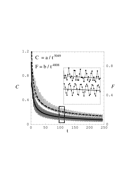
Figure 4: Evidence for approach to a spatially homogeneous background cosmology. The circumference ${\mathcal{C}}$ and force ${\mathcal{F}}$ are shown. The dashed and solid thick lines are power-law fits with the indicated exponents. The region inside the rectangle is shown in the inset. The lower curve (solid line or line with circles) represents ${\mathcal{C}}$ and the upper curve (dashed line or line with squares) represents ${\mathcal{F}}$.

For a reliable simulation it is then possible to compute ${\mathcal{C}}$ and ${\mathcal{F}}$ using Eqs. (87) and (90) respectively. These are shown in Fig. 4 along with power law fits to the data. A closeup of the oscillatory functions $\rho(t)$ and $\psi(t)$ (see Fig. 4b) argues that the larger discrepancy in ${\mathcal{F}}$ between the expected $t^{-1/2}$ and the observed decay is due to the greater difficulty in determining the centroid of the pattern. Similar decay as $t^{-1/2}$ is shown for other representative initial data in Fig. 5.

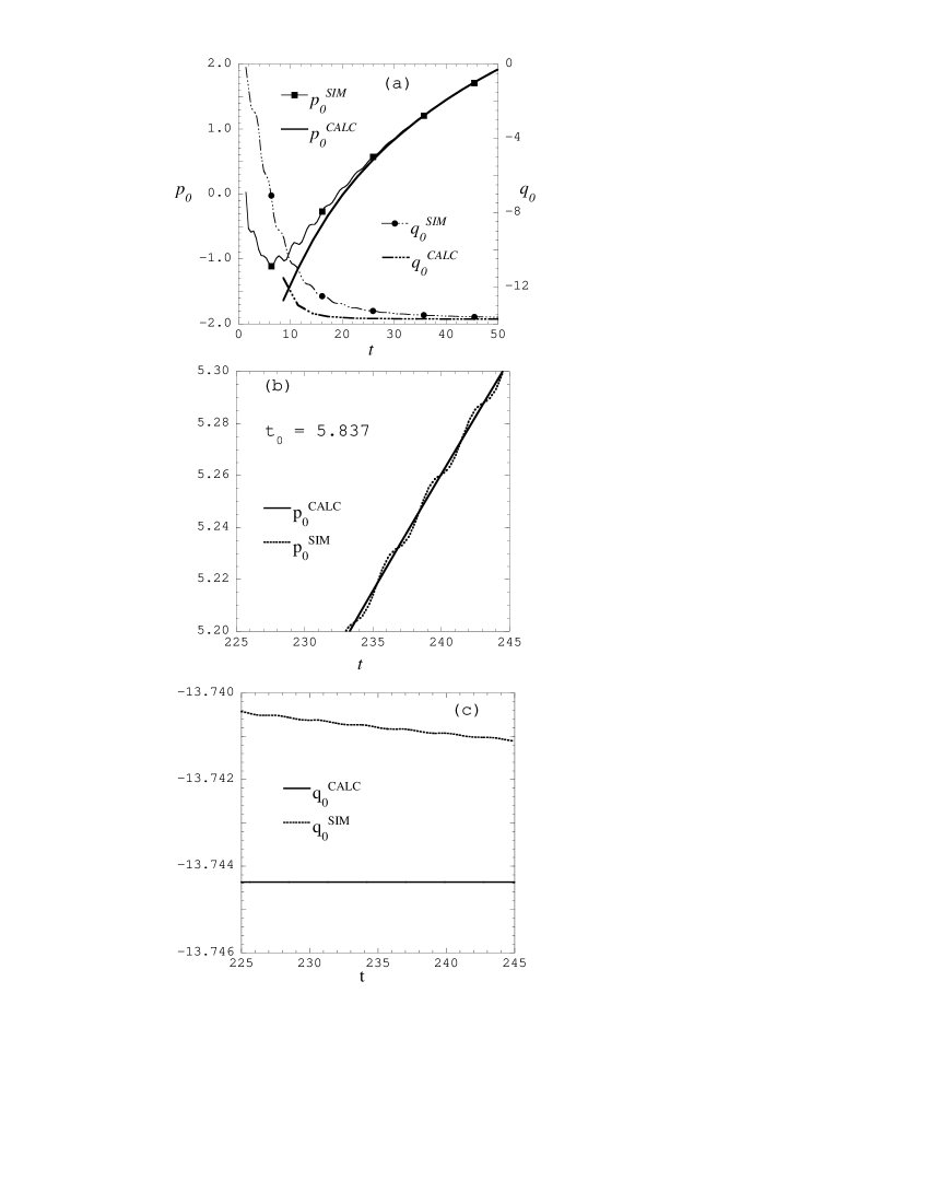
Figure 6: Predicting the asymptotic spatially homogeneous model. (a) The values of the spatially homogeneous modes, $\bar{p}$ of $P$ (solid line with squares) and $\bar{q}$ of $Q$ (dashed line with circles), are compared to $p_{0}$ and $q_{0}$ calculated from $\mu$, $\xi$, $v$, and the best fit to $t_{0}$. (b) Rescaling the time associated with given values of $p_{0}$ and $q_{0}$ until $p_{0}$ matches the center of $\bar{p}$. This occurs if $t_{0}=5.837$. (Note that the value of $t_{0}$ will change slightly as the match is made for increasing $t$, eventually reaching the “true” value at $t=\infty$.) (c) A comparison between $\bar{q}$ (dashed) and $q_{0}$ (solid) late in the simulation. Note that $\bar{q}$ is decaying to $q_{0}$ and that the difference is only a few parts in $10^{4}$.

If these solutions indeed decay to a spatially homogeneous background spacetime, it now becomes possible to identify the precise asymptotic behavior of $P$ and $Q$. Since $P$ and $Q$ are periodic functions on $[0,2\pi]$, it is always possible to compute the spatially homogeneous mode of the appropriate Fourier series. This mode for $P$ and $Q$ (say $\bar{p}$ and $\bar{q}$) contains the $\varepsilon^{0}$ solution as well as the spatially homogeneous modes of the order $\varepsilon^{n}$ solutions for $n\geq 2$. However, if the asymptotic forms given in Eqs. (62) and (63) indeed describe the solution, we require (as argued in Section III) that the higher order contributions to $\bar{p}$ and $\bar{q}$ should be oscillatory (and decaying) and should oscillate about the spatially homogeneous solutions $p_{0}$ and $q_{0}$ respectively. Evidence for such behavior is the following: The constants $A$, $B$, $C$ may be computed from the initial data and used to construct $\mu$, $\xi$, and $v$. This yields $p_{0}$ and $q_{0}$ as functions of $t/t_{0}$ where $t_{0}$ is as yet unknown. Fig. 6 shows that if $t_{0}$ is chosen to yield a best fit to (say) $\bar{p}$ late in the simulation, it also fits the correct average time dependence of $\bar{p}$ and yields the correct asymptotic behavior for $\bar{q}$. The fact that we can fit two functions with one adjustable parameter provides strong support that the computed $\mu$, $\xi$, $v$, and the fit $t_{0}$ define the correct asymptotic $P$ and $Q$.

Note that the time averaged values of $\bar{p}$ and $\bar{q}$ depart from $p_{0}$ and $q_{0}$ early in the simulation. This means that, although $\mu$, $v$, and $\xi$ are fixed by the initial data, $t_{0}$ does not have the value one would calculate from the initial data. This means that nonlinear interactions which are important early in the simulation influence (i.e. renormalize) the value of $t_{0}$ and thus the background spacetime.

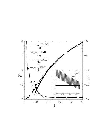
Figure 7: An alternative approach to the determination of $t_{0}$. The empirically determined $\tilde{p}_{0}$ (labeled $p_{0}^{EMP}$) and $\tilde{q}_{0}$ approach $p_{0}$ (labeled $p_{0}^{CALC}$) and $q_{0}$ as $\tilde{t}_{0}$ evolves toward $t_{0}$ (inset).

Also note that it is possible to evaluate $t_{0}$ without fitting by constructing $\tilde{p}$ and $\tilde{q}$ defined as the solutions (10) and (11) where $\mu$, $\xi$, and $v$ are those found from the initial data while $t_{0}$ is evaluated from $\bar{p}$, $\bar{q}$ at that time step. This procedure yields $\tilde{t}_{0}(t)$ which converges to $t_{0}$ as $t\to\infty$. Fig. 7 shows $\tilde{p}$, $\tilde{q}$, and $\tilde{t}_{0}$ compared to $p_{0}$, $q_{0}$, and $t_{0}$.

Fig. 8 shows the spatial average of $\lambda$ vs. $t$ for a representative simulation. The time dependence is clearly linear (and definitely not logarithmic). Also shown is the spatial average of the energy-like terms, ${\mathcal{E}}$ in Eq. (4), which are the “source” for $\lambda$. Detailed examination shows that the fluctuations in the source terms decay (as $1/t$) to the appropriate constant value.

The analysis of Sections III and IV and the numerical simulations have provided support for an asymptotic state described by gravitational waves of decaying amplitude propagating in a spatially homogeneous cosmology. Figures 9–14 illustrate the mechanism yielding this asymptotic state. In particular, the source terms ${\mathcal{S}}_{P}(t)$ and ${\mathcal{S}}_{Q}(t)$ must be driven to small amplitude if they are not small initially. Note that the exponential dependence on $P$ in ${\mathcal{S}}_{P}$ could be catastrophic if, for example, $P$ were to depend linearly on $t$. In fact, such linear behavior of $P$ is seen very early in the simulation in Fig. 11. There, the nonlinear terms then act as regulators (as described for the collapsing direction in Berger and Garfinkle (1998)) to suppress the linear behavior.

The consistency between the asymptotic behaviors of $P$, $Q$, and $\lambda$ found in the numerical simulations and those expected from the analysis in Sections III and IV suggests that the behavior found there for the nonlinear source terms ${\mathcal{S}}_{P}(t)$ and ${\mathcal{S}}_{Q}(t)$ on $p_{0}(t)$ and $q_{0}(t)$ must be correct—i.e. these terms decay as $1/t$ or faster yielding decaying perturbations $p_{n}^{(0)}$ and $q_{n}^{(0)}$ for $n\geq 2$ of $p_{0}$ and $q_{0}$ respectively. It is interesting to examine direct evaluation of the relevant terms during the simulation. Figures 9 and 10 illustrate respectively the component terms of ${\mathcal{S}}_{P}$ and ${\mathcal{S}}_{Q}$ (along with the corresponding $P$ and $Q$) for the entire simulation starting from the initial data of Fig. 1. Early in the simulation, nonlinear effects dominate. The term in ${\mathcal{S}}_{P}$, $V_{1}=\oint\,d\theta\,e^{2P}\,Q,_{t}^{2}$, in fact behaves as $B^{2}\,e^{-2P}$ (i.e. it is dominated by the constant of motion $B$) as is seen to be the case in Fig. 9 and, for more complicated initial data, in Fig. 11. Figures 10 and 12 illustrate the complicated evolution of the two terms in ${\mathcal{S}}_{Q}$ which, in the end, are seen to decay. Figures 13 and 14 show the evolution of ${\mathcal{S}}_{P}$ and ${\mathcal{S}}_{Q}$ early and late in the simulation (for the complicated initial data). Nonlinear effects are clearly significant early in the simulation. Late in the simulation, however, ${\mathcal{S}}_{P}$ and ${\mathcal{S}}_{Q}$ have decayed to small amplitudes with even smaller (by several orders of magnitude) time averages (see Fig. 14). This oscillatory (in time) behavior of the source terms means that any (positive or negative) growth in $P$ tends to produce a correction to reduce the magnitude of the growing term. Thus the time averages of these source terms represent their actual, negligible influence on the dynamics.

VI Conclusions

We have shown here that the asymptotic state of a class of expanding Gowdy models may be described quantitatively as decaying amplitude gravitational waves propagating in a spatially homogeneous background spacetime. Quantities such as the orbit circumference in the target space, ${\mathcal{C}}$, and generalized force, ${\mathcal{F}}$, are seen to decay to the background value of zero as $t^{-1/2}$ as predicted by perturbative methods. (After these results were obtained, Ringström was able to prove the form (88) for ${\mathcal{C}}$ for “small” initial data Ringström .) In addition, we have provided a prescription for construction of the asymptotic background spacetime.

Open questions concern the generality of the results discussed here. While the asymptotic behavior (62), (63) has been found for many sets of initial data for this class of Gowdy spacetimes, there is no guarantee that the parameter space of such data has been fully explored. (In this context, Ringström’s result for the decay of the gravitational wave amplitudes is quite encouraging.) One hopes that this will be settled with mathematical tools.

A more significant issue is whether or not other classes of spatially inhomogeneous cosmological spacetimes may be described in terms of matter and gravitational radiation with decreasing influence on a background spatially homogeneous cosmology. Most cosmological studies assume that the present universe may be described this way. Within the Gowdy models considered here, this type of description arises after a nonlinear regime which has an influence on the final state of the system.

Investigations of more general models are in progress. We note that, in contrast to the collapsing case where most types of “matter” are dynamically unimportant, every modification of the nature of the expanding model and its matter content affects the dynamics. Finally, we remark that a modification of the techniques used here have been applied to vacuum, general $T^{2}$ symmetric spacetimes (see Berger et al. (1997) for a description of these spacetimes). Results will be discussed elsewhere Berger and Isenberg .

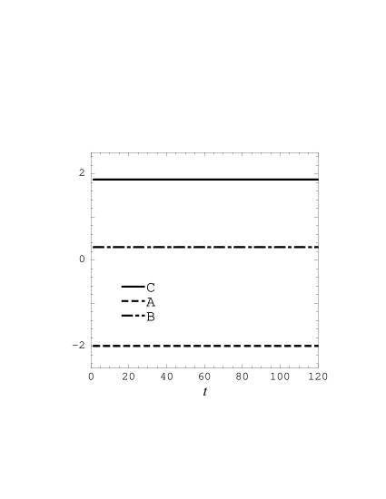
Figure 1: Constants of the motion $A$, $B$, and $C$ in a representative expanding Gowdy spacetime. Unless otherwise noted, all figures are constructed from a simulation with $P=1$, $P,_{t}=2\,+\,2\cos\theta$, $Q=\cos\theta$, $Q,_{t}=0.3$, and $\lambda=0.6\,e^{2}\,\cos\theta$ at $t=1$.

Figure 2: Fluctuations of $A$. On a fine numerical scale, numerical fluctuations in $A$ (which should be strictly constant) are visible. In the main graph, the three curves show (from top to bottom) fluctuations with spatial resolutions of 4096, 2048, and 1024 points respectively. Offsets have been added to the lower resolution values to allow display on the same graph. The inset shows the mean values where the spatial resolution increases from top to bottom over the same range in time. It is clear that numerical errors in the constant $A$ are converging to zero and that the mean value is also converging.

Figure 3: Integrands for $A$, $B$, and $C$ at a representative spatial point. While the constants $A$, $B$, and $C$ are preserved in the numerical simulation, the integrands $\tilde{A}$, $\tilde{B}$, and $\tilde{C}$ fluctuate wildly. Here they are rescaled to allow display on a single graph. The horizontal line represents the average values.

Figure 5: Decay of ${\mathcal{C}}$ (solid lines) and ${\mathcal{F}}$ (dashed lines) for three different expanding Gowdy models. The respective power-law fits are shown at the top of the graph.

Figure 8: Linear growth of $\lambda$. The dots represent every 20th point in the spatial average of $\lambda$ as computed using Eq. (4) in a numerical simulation. The solid line is $\bar{\lambda}=23.00\,+\,4.4969\,t$. Also shown is the energy-like spatial average of the source terms for $\lambda,_{t}$, which, while fluctuating, asymptote to a constant. Note the small range on the scale for ${\mathcal{E}}$. The thick solid line is ${\mathcal{E}}=4.4969\,+\,5.6388/t$.

Figure 9: Nonlinear fluctuations and the spatial average of $P$. The nonlinear terms $V_{1}=\oint d\theta\,e^{2P}Q,_{t}^{2}$ (thin solid line) and $V_{2}=\oint d\theta\,e^{2P}Q,_{\theta}^{2}$ (dashed line) are shown on a log-log plot (using the vertical axis labeled $NL$). The logarithmic time axis is used to emphasize the behavior during the early stages of the simulation when nonlinear effects are significant. For comparison, the spatial average of $P$ is also shown (thick solid line). Note that $V_{1}$ increases and $V_{2}$ decreases as $P$ decreases as expected if these terms are acting to regulate $P$.

Figure 10: Nonlinear fluctuations and the spatial average of $Q$. The nonlinear terms $W_{1}=2|\oint d\theta\,P,_{t}Q,_{t}|$ (thin solid line) and $W_{2}=2|\oint d\theta\,P,_{\theta}Q,_{\theta}|$ (dashed line) are shown on a log-log plot (using the vertical axis labeled $NL$). For comparison, the spatial average of $Q$ is also shown (thick solid line).

Figure 11: Nonlinear terms and the spatial average of $P$ early in the simulation. The nonlinear terms $V_{1}$ (thin solid line) and $V_{2}$ (dashed line) (see Fig. 9) are shown for $1\leq t\leq 6$ (using the vertical axis labeled $NL$). For comparison, the spatial average of $P$ is also shown (thick solid line). For this and subsequent figures, the initial data are $P=0$, $P,_{t}=2\,+\,2\cos\theta\,+\,0.5\cos(2\theta)\,+\,4\cos(5\theta)$, $Q=\cos\theta\,+\,2\cos(3\theta)\,+\,\cos(7\theta)$, $Q,_{t}=0.3$. Note that, as $P$ becomes increasingly negative early in the simulation, $V_{1}$ increases while $V_{2}$ decreases supporting the contention that the former evolves as $e^{-2P}$. Also note the qualitative similarities to Fig. 9 despite quite different initial data.

Figure 12: Nonlinear terms and the spatial average of $Q$ early in the simulation. The nonlinear terms $W_{1}$ (thin solid line) and $W_{2}$ (dashed line) (see Fig. 10) are shown for $1\leq t\leq 6$ (using the vertical axis labeled $NL$). For comparison, the spatial average of $Q$ is also shown (thick solid line). The horizontal line indicates zero for the nonlinear terms. Note that the difference in initial data leads to qualitative differences in evolution in Figs. 10 and 12.

Figure 13: Nonlinear source terms $S_{P}(t)$ (solid line) and $S_{Q}(t)$ (dashed line) early in the simulation. Note how quickly these terms approach a state where they oscillate more or less symmetrically about zero.

Figure 14: Nonlinear source terms $S_{P}(t)=V_{1}\,-\,V_{2}$ (solid line) and $S_{Q}(t)=W_{2}\,-\,W_{1}$ (dashed line) late in the simulation. Note the small amplitude of these terms and that their time averages are very close to zero ($9\times 10^{-4}$ and $2\times 10^{-5}$ respectively).