Convergence and stability in numerical relativity

Abstract

It is often the case in numerical relativity that schemes that are known to be convergent for well posed systems are used in evolutions of weakly hyperbolic (WH) formulations of Einstein’s equations. Here we explicitly show that with several of the discretizations that have been used through out the years, this procedure leads to non-convergent schemes. That is, arbitrarily small initial errors are amplified without bound when resolution is increased, independently of the amount of numerical dissipation introduced. The lack of convergence introduced by this instability can be particularly subtle, in the sense that it can be missed by several convergence tests, especially in 3+1 dimensional codes. We propose tests and methods to analyze convergence that may help detect these situations.

Convergence is a central element of any numerical simulation. It refers to the property that if one refines the simulation by adding more points to the grid, numerical errors should diminish. In the limit of zero spacing, they should go to zero and one should get the exact solution. Having a convergent code is a key element for numerical simulations to have predictive power: although one will always be limited in practice to a finite number of points in the grid, one can extrapolate the results for more and more refined simulations and have a very good approximation to the true (continuum) results. Codes that do not converge produce answers that, even if they remain finite (at least for a while), have little predictive power: there generically is no way to know if the solutions found approximate the desired continuum solution.

In this paper we want to emphasize that discretization schemes that yield convergent code for strongly hyperbolic (SH) systems of equations do not necessarily do so for weakly hyperbolic (WH) or completely ill posed (CIP) systems. The relevance of this observation is that several formulations of the Einstein evolution equations commonly used in numerical relativity, including, for example, the Arnowitt–Deser–Misner (ADM) ADM and Baumgarte–Shapiro–Shibata–Nakamura (BSSN) BSSN formulations with fixed lapse and shift, are not SH.

We concretely prove that a simple system of linear WH equations with constant coefficients, when discretized with either the iterated Crank–Nicholson (ICN) with fixed number of iterations or second order Runge–Kutta (2RK) methods, leads to unconditionally unstable codes, even if numerical dissipation is explicitly added. This simple system of equations is related to the equations one encounters in the WH formulations of general relativity. It therefore strongly suggests that these formulations should produce code that is not convergent. The lack of convergence is of a particularly pernicious nature, since in the WH case it might grow slower than the “usual” von-Neumann numerical instability. It is such that if one tests the code with stationary solutions (for instance simulating a single black hole) and performs convergence tests, one could easily be confused into believing one has convergent code.

Consider a linear system of $m$ partial differential equations in $m$ variables of the form

$$\partial_{t}v=A\partial_{x}v\;,$$ (1)

where $A$ is a constant $m\times m$ matrix and $v=(v_{1},\ldots,v_{m})^{T}$. The system is SH if $A$ has real eigenvalues and is diagonalizable, WH if it has real eigenvalues but is not diagonalizable, and CIP if it has complex eigenvalues.

The iterated Crank–Nicholson (ICN) method is an explicit approximation to the (implicit) Crank–Nicholson method first proposed by Choptuik. In this proposal the number of iterations is not fixed but, instead, might depend on the spatial gridpoint and time step . A different notion of ICN is to a priori fix the number of iterations ICN . Teukolsky ICN showed that for the advective equation, $\partial_{t}{v}=\partial_{x}v$ (which is SH), such scheme was stable if one used $2,3,6,7,10,11,\ldots$ iterations (one iteration corresponds to the 2RK method). This paper seeks to extend this proof to more general systems of equations, including explicit artificial viscosity.

A difference scheme is said to be stable with respect to a given norm if there exist positive constants $\Delta x_{0}$ and $\Delta t_{0}$ and $f(t)$ such that $\|u^{n}\|\,\leq\,f(t)\,\|u^{0}\|\,,$ for $0<\Delta x\leq\Delta x_{0}$, $0<\Delta t\leq\Delta t_{0}$, and $t=n\Delta t$ where $u^{n}$ is the numerical solution at time $t$ and $u^{0}$ the initial data. That is, the growth of the solution is bounded by some function of time $f(t)$ that is independent of the initial data and resolution. Some schemes are only conditionally stable. This means that a relationship between $\Delta t$ and $\Delta x$ is needed for stability. Through Lax’s theorem, numerical stability in this sense is equivalent to convergence, provided the scheme is consistent.

Working in Fourier space and writing explicitly the solution at time $t$ in terms of the amplification matrix $Q$, $\hat{u}^{n}=Q^{n}\hat{u}^{0}$ yields a necessary condition for stability: the von-Neumann condition (VNC). It states that, for the cases considered in this paper, the spectral radius $\rho(Q)$ of $Q$ (the maximum eigenvalue in norm) is not greater than one. If this condition is not satisfied, a numerical instability that grows like $\exp{(n\mu)}$, with $\mu>0$ a constant, is present. A well known example of this instability is the forward in time, centered in space scheme for the advective equation. It is sometimes thought that the VNC is not only necessary but also sufficient for stability. This often leads to (wrongly) concluding that a discretization for a WH system is stable based on an discrete analysis for the advection or wave equation. The VNC is sufficient only if $Q$ can be diagonalized by a similarity transformation whose norm, and that of its inverse, has an upper bound that is independent of resolution kreiss . An observation that will be important for the stability analysis below is that, for the cases we are discussing, $Q$ is diagonalizable if and only if $A$ is. Therefore, in the WH case the VNC will not be sufficient for stability.

On the other hand, if the system is SH $A$ is diagonalizable (with real eigenvalues) and so is $Q$. Working in the diagonal basis we then have an uncoupled system of $m$ equations for the $m$ grid functions. Repeating Teukolsky’s analysis for the ICN scheme, this system is stable if $\rho(A)\lambda\leq 2$ ($\lambda=\Delta t/\Delta x$ is the Courant factor) and the number of iterations is $p=2,3,6,7,10,11,\ldots$, if no explicit dissipation is added. In evolutions of SH equations, the addition of dissipation may help stabilize schemes that are otherwise unstable. For example, the VNC for the 2RK case with third order dissipation is

$$(\rho(A)\lambda)^{4}\leq 8\lambda\tilde{\sigma}\leq 1\;,$$ (2)

where $\tilde{\sigma}$ is the dissipation parameter. Since $Q$ is diagonal, this condition is necessary and sufficient for stability.

Below we will explicitly prove that for CIP or WH cases the ICN and 2RK methods are unstable, independently of the amount of dissipation, number of iterations and Courant factor. Although our results are only proven for a system of linear equations with constant coefficients, they are significant in several ways for numerical relativity. First of all, if one considers situations that are small perturbations off Minkowski spacetime, then a system of equations identical to the one we considered does appear in the linearized Einstein equations written in first order form in space and time if the system of evolution equations used is WH or CIP. Since far away from binary black holes the spacetime is approximately flat, this situation does arise in realistic simulations. Could non-linearities change our conclusions? It is possible, but unlikely. Usually when instabilities are established for linear systems the addition of non-linear terms only makes instabilities worse kreiss .

The type of lack of convergence differs in the CIP and WH case. In the CIP case the VNC is easily violated, codes crash very fast and non-convergence is easy to spot. In the WH case the VNC may be satisfied and crashes may occur very late (if they occur at all). If one performs routine convergence analyses in the region before the crash one might appear to see convergence, especially if the initial data has few (and low) frequency components, unless one increases enough the resolution or runs for long enough time.

We now show that these different types of lack of convergence do appear in numerical relativity simulations, even in very simple 1D ones with periodic boundary conditions. We have performed non-linear evolutions of a plane gauge wave spacetime (that is, the spacetime is flat, though in a time-dependent slicing),

$$ds^{2}=e^{A\sin{(t+x)}}(-dt^{2}+dx^{2})+dy^{2}+dz^{2}\;.$$ (3)

Figure 1 shows results of an evolution using 2RK with $\sigma=1/2,0,-1/2$ in the Einstein–Christoffel (EC) system ec of evolution equations. The latter is a symmetric-hyperbolic reformulation of Einstein’s evolution equations that includes a parameter $\sigma$ that densitizes the lapse. In the EC formulation, $\sigma=1/2$, but by tuning this parameter we can make the system WH ($\sigma=0$) or CIP ($\sigma=-1/2$). The whole $30$ equations of the EC system are evolved, but all quantities are assumed to depend only on $t$ and $x\in[-\pi,\pi]$. The Courant factor is set to $1/2$, the dissipation parameter to $\tilde{\sigma}=0.02$, and the evolution is followed for $1,000$ crossing times. In the SH case the code is convergent for all resolutions tested, see stability for a detailed discussion. On the other hand, in the same code with $\sigma=-1/2$ a lack of convergence becomes apparent immediately (before one crossing time), the errors become bigger and the code crashes earlier as resolution is increased. In the WH case the code is also not convergent but the effect is less noticeable, since with the chosen values of dissipation and Courant factor the VNC, Eq.(2), is satisfied.

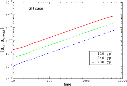
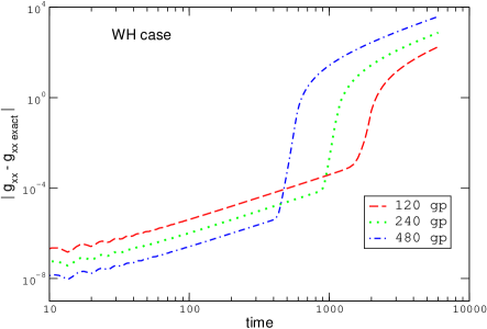
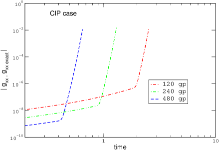
Figure 1: $L_{2}$ norm of the errors for the metric in the SH, WH and CIP cases.

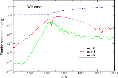
Figure 2: The lack of convergence in the particular WH case considered is triggered by non-zero frequency modes that are suppressed in the initial data, but grow exponentially. Notice that after the lack of convergence becomes obvious (at $t=2000$ for this resolution) no further exponential growth takes place and the code does not crash, in the example we are considering.

If one performed only a few runs, with, say $120$ and $240$ gridpoints as is typical in 3D convergence studies, one would have to wait for around $150$ crossing times in order for the lack of convergence in this WH example to become obvious. To put these numbers in context, suppose one had a similar situation in a 3D black hole evolution. Suppose the singularity is excised, with the inner boundary at $r=M$ and the outer boundary at $20M$. In this case $120$ and $240$ gridpoints correspond to grid spacings of, approximately, $M/5$ and $M/10$, respectively. If one had to evolve up to $150$ crossing times in order to notice the lack of convergence, that would correspond to $t\approx 3000M$, which is more than what present 3D evolutions typically last. One could therefore be misled to think that the code is convergent. Repeating the same runs with an initial data with more frequencies (say, a non-stationary black hole) would make the instability manifest in a shorter timescale. By making a spatial Fourier decomposition (Figure 2) of the numerical solution, we have found that in the WH and CIP cases there are always non-zero frequency modes growing exponentially from the very beginning, though sometimes starting at truncation error. By performing such decomposition one can detect that the code is not convergent much before this becomes obvious in the overall errors.

We have done simulations with different spectral distributions on the initial data, different number of iterations in the ICN method, different Courant factors, and different values of dissipation. The time and resolution at which the numerical instability becomes obvious depends on all these factors, but lack of convergence is always present in the CIP and WH cases, while the SH runs do converge. Too much dissipation violates the VNC, resulting in a more severe instability and this is immediately seen in numerical experiments, see stability for details.

We have also found similar results performing simulations with the same initial data but with Kidder-Scheel-Teukolsky’s many parameter family of formulations of Einstein’s equations kst , leaving all parameters fixed and changing only one of them at a time, achieving different levels of hyperbolicity. In particular, we have found lack of convergence in the ADM equations as well (which is a subsytem of this family).

The results presented in this paper do not represent a special feature of the ICN method but instead, only reflect the fact that the definition of numerical stability is just a discrete version of well posedness. Therefore, difference schemes approximating ill posed problems can be expected to be non-convergent. In the absence of boundaries this is the case for CIP or, generically, WH formlations. If there are boundaries, strong hyperbolicity is not enough and extra care has to be taken in order to guarantee well posedness; wrong boundary conditions not only lead to inconsistencies but also to lack of convergence (see, e.g., tadmor ).

Although it is not possible to prove in a definitive way that a code is convergent only by numerical experiments, the previous examples suggest some of the pathologies that one should look for. Namely, Fourier modes that are not convergent but that are very small for a while, since they are initially suppressed. Also, notice from the WH simulations above shown that a code does not need to crash nor exhibit violent growth in order not to converge. The main lesson learned from this paper is that one should exercise significant care in numerical simulations before empirically concluding that the simulation is convergent, especially if the formulation of Einstein’s equations used is not SH or its level of hyperbolicity is unknown.

We wish to thank D. Arnold, M. Choptuik, P. Laguna, L. Lehner, M. Miller, R. Price, O. Reula, and S. Teukolsky for comments. This work was supported in part by NSF grant PHY9800973, the Horace Hearne Jr. Institute for Theoretical Physics, the Swiss National Science Foundation, and Fundación Antorchas.

Proof of non-convergence for CIP and WH cases: A usual way of discretizing the right hand side of Eq.(1) is using centered differences plus third order explicit dissipation. By this one means solving $\partial_{t}v=Cv/\Delta t$, with $C=A\lambda\delta_{0}/2-\tilde{\sigma}\lambda\delta^{4}$, where $I$ is the identity matrix, $\delta_{0}v_{k}=v_{k+1}-v_{k-1}$, and $\delta^{4}v_{k}=v_{k+2}-4v_{k+1}+6v_{k}-4v_{k-1}+v_{k-2}$. This is equivalent to discretizing $\partial_{t}v=A\partial_{x}v-I\tilde{\sigma}(\Delta x)^{3}\partial_{x}^{4}v$ using centered differences (using first order dissipation in our proof, i.e. discretizing $\partial_{t}v=A\partial_{x}v+\tilde{\sigma}\Delta x\partial_{x}^{2}v$, gives similar results).

The ICN method with $p$ iterations for the partial differential equation (1) can be written as

$$v^{n+1}_{k}=\left(1+2\sum_{j=1}^{p+1}\frac{C^{j}}{2^{j}}\right)v^{n}_{k}\;,$$ (4)

where $v_{k}^{n}=(v_{1\,k}^{n},\,\ldots,v_{m\,k}^{n})^{T}$. The index $n$ corresponds to the time step and $k$ to the spatial mesh point. Since we are considering an initial value problem on all of ${\sf R\rule{0.6458pt}{6.45831pt}\hskip 3.87495pt}$, $-\infty<k<+\infty$ (our proof can be easily modified for periodic boundary conditions, and the results are the same).

In order to analyze stability we work in the basis in which $A$ takes its canonical form. That is, one multiplies both sides of Eq.(4) by $T$, where $TAT^{-1}=J$ has the canonical Jordan form, and analyzes the equation

$$u^{n+1}_{k}=\left(1+2\sum_{j=1}^{p+1}\frac{L^{j}}{2^{j}}\right)u^{n}_{k}\;,$$ (5)

where $L=TCT^{-1}=J\lambda\delta_{0}/2-I\tilde{\sigma}\lambda\delta^{4}$. Any conclusions regarding stability will hold as well for the original variable $v$. Working in Fourier space, $u_{k}=\int_{-\pi}^{\pi}\exp{(ik\xi)}\hat{u}(\xi)d\xi$, $Q=1+2\sum_{j=1}^{p+1}{\hat{L}^{j}}/{2^{j}}$ and $\hat{L}=J\lambda i\sin(\xi)-16\tilde{\sigma}\lambda\sin^{4}(\xi/2)$.

If the system is CIP, $J$ has at least one complex eigenvalue $c$, say $J_{11}=c$. In this case, $\hat{L}_{11}=c\lambda i\sin(\xi)-16\tilde{\sigma}\lambda\sin^{4}(\xi/2)$, and the eigenvalue $Q_{11}$ has norm $1-\lambda Im(c)\xi+O(\xi^{2})$. Therefore, the VNC is violated for sufficiently small $\xi$ with the appropriate sign and the scheme is unconditionally unstable, as expected.

If the system is WH then $J$ has at least one Jordan block and so does $Q$. In this basis all the Jordan blocks are uncoupled and we can consider one at a time. We assume there is one block of dimension $2\times 2$ (the proof actually holds for higher dimensionality as well). The canonical form for such a block, the resulting amplification matrix, and its n-th power are

$$J=\left(\begin{array}[]{cc}c&1\\ 0&c\end{array}\right),\,Q=\left(\begin{array}[]{cc}a&b\\ 0&a\end{array}\right),\,Q^{n}=\left(\begin{array}[]{cc}a^{n}&a^{n-1}nb\\ 0&a^{n}\end{array}\right)\;.$$

Suppose the VNC $|a|\leq 1$ is satisfied (this rules out the $p=0$ case), we will show that the scheme is still unstable. Consider as initial data a small perturbation of the form

$${u}^{0}_{0}=(0,2\pi\epsilon)^{T}\;\;\;,\;\;\;u^{0}_{k}=(0,0)^{T}\mbox{ otherwise}$$ (6)

with $\epsilon$ arbitrary small. In Fourier space we have $\hat{u}^{0}(\xi)=\epsilon(0,\,1)^{T}$ for all $\xi$. The solution at time $t=n\Delta t$ is, then, $\hat{u}^{n}=\epsilon(a^{n-1}nb,\,a^{n})^{T}$. We will show that its norm grows without bound when the number of gridpoints is increased (while keeping the time and Courant factor fixed). We first notice that ($n_{2}\equiv 2n-2$),

$$\frac{\|u^{n}\|^{2}}{\|u^{0}\|^{2}}=\int_{-\pi}^{\pi}\!\!\!\!\left(n^{2}|a|^{n_{2}}|b|^{2}+|a|^{2n}\right)\,{d\xi\over 2\pi}\geq n^{2}\int_{-\pi}^{\pi}|a|^{n_{2}}|b|^{2}{d\xi\over 2\pi}.$$ (7)

Expressions $|a|^{2}$ and $|b|^{2}$ are analytic functions of $\xi$ with Taylor expansion $|b|^{2}=\lambda^{2}[\xi^{2}+O(\xi^{4})]\,$ and $|a|^{2}=1-[2\tilde{\sigma}\lambda+d(c\lambda)^{4}]\xi^{4}+O(\xi^{6})$, with $d=-1$ for $p=1$, $d=1$ for $p=2$, and $d=0$ otherwise. From these expansions one can see that, for all $p$, there are positive constants $\alpha$ and $\rho$ such that

$$|a(\xi)|^{2}\geq 1-\alpha\xi^{4}\geq 0\;\;\;,\;\;\;|b(\xi)|^{2}\geq\rho^{2}\xi^{2}\geq 0\;,$$ (8)

for small enough $\xi$, say $|\xi|\leq\epsilon_{1}$. For $n>1$ and small enough $\xi$, say $|\xi|\leq\epsilon_{2}$,

$$|a(\xi)|^{2n}\geq 1-n\alpha\xi^{4}\geq 0\;,$$ (9)

where the last inequality holds for $|\xi|\leq(n\alpha)^{-1/4}$, provided that $n$ is large enough so that $(n\alpha)^{-1/4}\leq\min(\epsilon_{1},\epsilon_{2})$. Using bounds (8,9) and the VNC in inequality (7) gives

$$\frac{\|u^{n}\|^{2}}{\|u^{0}\|^{2}}\geq n^{2}\int_{-(n\alpha)^{-1/4}}^{(n\alpha)^{-1/4}}\!\!\!\!(1-n\alpha\xi^{4})\rho^{2}\xi^{2}\,\frac{d\xi}{2\pi}=\frac{4}{21\pi}\frac{\rho^{2}}{\alpha^{3/4}}n^{5/4}$$

which diverges for $n\rightarrow\infty$. This shows that in the WH case the ICN and 2RK schemes are unstable, independent of the amount of dissipation. In fact, by examining $|a(\xi=\pi)|$, one can see that a necessary condition for the VNC (for any number of iterations) is $0\leq\tilde{\sigma}\lambda\leq 1/8$. Adding too much dissipation violates the VNC and the instability becomes worse.

Perturbations like that of (6) are to be expected in a numerical simulation due to truncation or roundoff errors. For high enough resolution, such a perturbation will be amplified without bound, spoiling any convergence. One expects that in the non-constant coefficient or in the non-linear case the rate of growth of the instability with number of gridpoints will be even faster (see example in page 216 of kreiss ), as in figure 2.

References

- (1) R. Arnowitt, S. Deser, C. Misner, in Gravitation: An Introduction to Current Research, L. Witten, ed. (John Wiley, New York, 1962)
- (2) T. W. Baumgarte and S. L. Shapiro, Phys. Rev. D 59, 024007 (1999); M. Shibata and T. Nakamura, Phys. Rev. D 52 (1995) 5428.
- (3) S. A. Teukolsky, Phys. Rev. D 61, 087501 (2000)
- (4) B. Gustafsson, H.O. Kreiss, J. Oliger, Time dependent problems and difference methods (Wiley, New York, 1995).
- (5) A. Anderson and J. W. York, Phys. Rev. Lett. 81, 1154 (1998)
- (6) G. Calabrese, J. Pullin, O. Sarbach, and M. Tiglio, gr-qc/0205073.
- (7) L. E. Kidder, M. A. Scheel and S. A. Teukolsky, Phys. Rev. D 64, 064017 (2001).
- (8) E. Tadmor, The unconditional instability of inflow-dependent boundary conditions in difference approximations to hyperbolic systems, Math. of Computation, 41, 309 (1983).